use of aria to simulate laser weld pool dynamics for...

SANDIA REPORTSAND2007-5870Unclassified Unlimited ReleasePrinted September 12, 2007

Use of Aria to Simulate Laser WeldPool Dynamics for Neutron GeneratorProduction

Patrick K. Notz, David R. Noble, Mario J. Martinez, Andrew M. Kraynik

Prepared bySandia National LaboratoriesAlbuquerque, New Mexico 87185 and Livermore, California 94550

Sandia is a multiprogram laboratory operated by Sandia Corporation,a Lockheed Martin Company, for the United States Department of Energy’sNational Nuclear Security Administration under Contract DE-AC04-94-AL85000.

Approved for public release; further dissemination unlimited.

Issued by Sandia National Laboratories, operated for the United States Department of Energy by SandiaCorporation.

NOTICE: This report was prepared as an account of work sponsored by an agency of the United StatesGovernment. Neither the United States Government, nor any agency thereof, nor any of their employees,nor any of their contractors, subcontractors, or their employees, make any warranty, express or implied,or assume any legal liability or responsibility for the accuracy, completeness, or usefulness of any infor-mation, apparatus, product, or process disclosed, or represent that its use would not infringe privatelyowned rights. Reference herein to any specific commercial product, process, or service by trade name,trademark, manufacturer, or otherwise, does not necessarily constitute or imply its endorsement, recom-mendation, or favoring by the United States Government, any agency thereof, or any of their contractorsor subcontractors. The views and opinions expressed herein do not necessarily state or reflect those ofthe United States Government, any agency thereof, or any of their contractors.

Printed in the United States of America. This report has been reproduced directly from the best availablecopy.

Available to DOE and DOE contractors fromU.S. Department of EnergyOffice of Scientific and Technical InformationP.O. Box 62Oak Ridge, TN 37831

Telephone: (865) 576-8401Facsimile: (865) 576-5728E-Mail: [email protected] ordering: http://www.osti.gov/bridge

Available to the public fromU.S. Department of CommerceNational Technical Information Service5285 Port Royal RdSpringfield, VA 22161

Telephone: (800) 553-6847Facsimile: (703) 605-6900E-Mail: [email protected] ordering: http://www.ntis.gov/help/ordermethods.asp?loc=7-4-0#online

DE

PA

RT

MENT OF EN

ER

GY

• • UN

IT

ED

STATES OFA

M

ER

IC

A

2

SAND2007-5870Unclassified Unlimited ReleasePrinted September 12, 2007

Use of Aria to Simulate Laser Weld Pool Dynamicsfor Neutron Generator Production

Patrick K. Notz, David R. Noble, Mario J. Martinez, Andrew M. KraynikSandia National Laboratories

P.O. Box 5800Albuquerque, NM 87185

Abstract

This report documents the results for the FY07 ASC Integrated Codes Level 2 Mile-stone number 2354. The description for this milestone is, “Demonstrate level set freesurface tracking capabilities in ARIA to simulate the dynamics of the formation andtime evolution of a weld pool in laser welding applications for neutron generator pro-duction.” The specialized boundary conditions and material properties for the laserwelding application were implemented and verified by comparison with existing, two-dimensional applications. Analyses of stationary spot welds and traveling line weldswere performed and the accuracy of the three-dimensional (3D) level set algorithm isassessed by comparison with 3D moving mesh calculations.

3

Contents

Contents 4

List of Figures 6

1 Introduction 9

1.1 Laser Welding . . . . . . . . . . . . . . . . . . . . . . . . . . . . . . . . . . . . . . . . . . . . . 9

1.2 Milestone . . . . . . . . . . . . . . . . . . . . . . . . . . . . . . . . . . . . . . . . . . . . . . . . . 10

2 Governing Equations and Boundary Conditions 13

2.1 The Physical Model . . . . . . . . . . . . . . . . . . . . . . . . . . . . . . . . . . . . . . . . . 13

2.2 Governing Equations . . . . . . . . . . . . . . . . . . . . . . . . . . . . . . . . . . . . . . . . 14

2.3 Boundary Conditions . . . . . . . . . . . . . . . . . . . . . . . . . . . . . . . . . . . . . . . . 15

2.4 Material Models . . . . . . . . . . . . . . . . . . . . . . . . . . . . . . . . . . . . . . . . . . . . 18

3 Computational Algorithms 21

3.1 Interface Tracking . . . . . . . . . . . . . . . . . . . . . . . . . . . . . . . . . . . . . . . . . . 21

3.2 The Level Set Method . . . . . . . . . . . . . . . . . . . . . . . . . . . . . . . . . . . . . . . 22

3.3 ALE Mesh Motion . . . . . . . . . . . . . . . . . . . . . . . . . . . . . . . . . . . . . . . . . . 24

3.4 The Finite Element Method . . . . . . . . . . . . . . . . . . . . . . . . . . . . . . . . . . 25

3.5 Pressure Stabilization . . . . . . . . . . . . . . . . . . . . . . . . . . . . . . . . . . . . . . . 26

3.6 Adaptive Mesh Refinement . . . . . . . . . . . . . . . . . . . . . . . . . . . . . . . . . . . 26

4 Results 29

4.1 Comparisons Between Goma and Aria Weld Simulations . . . . . . . . . . . 29

4.2 Comparisons with Spot Weld Experiments . . . . . . . . . . . . . . . . . . . . . . 29

4

4.3 Comparisons Between ALE and Level Set Algorithms . . . . . . . . . . . . . 34

4.4 Demonstration Calculation: 3D Line Weld . . . . . . . . . . . . . . . . . . . . . . 36

5 Recommendations for Future Work 43

5.1 Linear Tetrahedral Elements are Preferred . . . . . . . . . . . . . . . . . . . . . . 43

5.2 Adaptivity is Essential for Efficiency and Accuracy . . . . . . . . . . . . . . . 43

5.3 Support for Discontinuous Fields at Interfaces . . . . . . . . . . . . . . . . . . . 44

5.4 Improved Level Set Performance . . . . . . . . . . . . . . . . . . . . . . . . . . . . . . 44

Appendix

A Example input Files 45

A.1 Cubit Journal File . . . . . . . . . . . . . . . . . . . . . . . . . . . . . . . . . . . . . . . . . . 45

A.2 Aria Input File . . . . . . . . . . . . . . . . . . . . . . . . . . . . . . . . . . . . . . . . . . . . . 46

References 53

5

List of Figures

2.1 Schematic diagram of a laser spot weld. Lx, Ly and Lz are the geometrydimensions and Rw is the weld pool radius which is a function of time t. 14

2.2 The vapor cooling energy flux qc as a function of temperature. . . . . . . . 16

2.3 The vapor recoil pressure pr as a function of temperature. . . . . . . . . . . . 17

2.4 The viscosity µ as a function of temperature. The large values of µ atlower temperatures simulate the unmelted steel. . . . . . . . . . . . . . . . . . . . 19

3.1 A plot of the regularized Heaviside (Eq. 3.1) and delta (Eq. 3.2)functions for an interfacial width α = 1. . . . . . . . . . . . . . . . . . . . . . . . . . . 23

4.1 Weld pool shape and temperature distribution (2D) at 1 ms in stainlesssteel SS304L. . . . . . . . . . . . . . . . . . . . . . . . . . . . . . . . . . . . . . . . . . . . . . . . . 30

4.2 Comparison of surface shear velocity components at 1 ms for a 2D spotweld simulation. . . . . . . . . . . . . . . . . . . . . . . . . . . . . . . . . . . . . . . . . . . . . . 30

4.3 Comparison of surface temperature profile at 1 ms for a 2D spot weldsimulation. . . . . . . . . . . . . . . . . . . . . . . . . . . . . . . . . . . . . . . . . . . . . . . . . . 31

4.4 Weld profiles in stainless steel SS304L with Argon as shield gas. Theprofile in red is from the experiments which is compared to the tem-perature profiles in black. The coolest isotherm depicts liquidus. . . . . . . 32

4.5 Weld profiles in stainless steel SS304L with air as shield gas. The profilein red is from the experiments which is compared to the temperatureprofiles in black. The coolest isotherm depicts liquidus. . . . . . . . . . . . . . 33

4.6 Weld pool shape and temperature profile for a 3D ALE simulation. . . . 35

4.7 Weld pool shape and temperature profile for a 3D ALE simulation withthe ambient air phase simulated. . . . . . . . . . . . . . . . . . . . . . . . . . . . . . . . . 35

4.8 Weld pool shape and temperature profile for a 3D ALE simulation withthe ambient air phase simulated. Here, the pressure is allowed to bediscontinuous at the liquid/gas interface. . . . . . . . . . . . . . . . . . . . . . . . . . 36

6

4.9 Weld pool shape and temperature profile for a 3D level set simulationwith α = 4× 105, nα = 4 and hI = 1× 10−5. . . . . . . . . . . . . . . . . . . . . . . 37

4.10 Weld pool shape and temperature profile for a 3D level set simulationwith α = 2× 105, nα = 4 and hI = 0.5× 10−5. . . . . . . . . . . . . . . . . . . . . 37

4.11 Weld pool shape and temperature profile for a 3D level set simulationwith α = 1× 105, nα = 4 and hI = 0.25× 10−5. . . . . . . . . . . . . . . . . . . . 38

4.12 Volume of the liquid (metal) phase as a function of time as predictedby the ALE and level set (LS) simulations. Physically, the volume ofthis phase should be constant for all times. These results illustratethe fictitious mass loss over time due to a continuous pressure for bothALE and LS simulation with varying interfacial elements sizes. . . . . . . . 38

4.13 Temperature distributions and weld pool shapes at three instances dur-ing a moving line weld using the level set algorithm. . . . . . . . . . . . . . . . . 40

4.14 Temperature distributions and weld pool shapes at three instances dur-ing a moving line weld using the ALE algorithm. . . . . . . . . . . . . . . . . . . 41

7

Chapter 1

Introduction

1.1 Laser Welding

Laser welding is a fusion welding technique which is achieved by focusing a veryhigh power density beam on a very fine spot. In contrast to other common weldingtechniques, laser welding does not depend solely on conduction for achieving weldpenetration. Initially, a large percentage of the beam energy is reflected, since mostmetals are good reflectors. However, the absorbed energy quickly produces an energyabsorbing ionized metal vapor, which rapidly accelerates the absorption of energy.The laser energy is not only absorbed on the surface, but to a depth into the work-piece. With high energy lasers, this leads to the development of a so-called keyhole –essentially a deep and narrow cavity drilled by the laser energy. Laser light is thoughtto be further scattered in the keyhole, thereby increasing the coupling of the laserenergy into the workpiece.

Major attributes of laser welding are that it produces deep and narrow welds, withminimal collateral heating of workpieces, and it can be performed at high produc-tion rates. The laser can be narrowly and precisely focused, so that very precise andcompact welds can be made, making laser welding ideal for joining miniature andintricate parts. Welds can be made very close to heat-sensitive components, suchas glass-to-metals seals or other electronic circuits, while minimizing thermal distor-tions. Laser welding permits welding speeds of several meters per minute, with atotal heat input that is much lower than other conventional techniques such as arcwelding. These attributes make laser welding an ideal joining method in manufactur-ing of components and subsystems at SNL. Laser welding has become a key joiningprocess used extensively in manufacturing and assembling of critical components inthe neutron generator, as well as in current and future life extension programs for allthe weapons systems. Nearly every current SNL component uses laser welds. SNLapplications include fireset housings, inertial switches, fuses, detonators, and otherexplosive components.

Laser welding is a challenging multiphysics problem requiring complex 3D modelsutilizing massively parallel algorithms to enable high fidelity solutions. Major chal-lenges in laser welds for weapons manufacturing include porosity formation and weld

9

morphology, especially large variations in weld shape/volume in the presence of sur-face active shield gases. Modeling and simulation in combination with experimentcan provide an effective (often the only) means to understand and control laser weld-ing to meet design specifications. Having a predictive capability for virtual weldingis critical for enabling agile manufacturing, a responsive infrastructure and supportsthe SNL vision of a science-based engineering transformation of system development.

The aforementioned attributes notwithstanding, there remains much room for im-provement of the laser welding process. The weld quality is strongly affected byoperational settings, such as weld speed, pulse frequency (in pulsed laser welding),and shield gas. Some issues include laser coupling problems, porosity formation, andthermal distortions. In addition to solving these operational issues, the long-rangegoal of research in laser welding is to develop the ability to model weld morphologyand weld integrity from basic principles.A fundamental goal of modeling is to provideunderstanding of how the altered grain structure of laser welds is associated with thefinal mechanical properties of the welded systems. Experiences such as mechanicalfailures occurring at welded joints indicate that the mechanical properties of weldedmaterial are often significantly different from unwelded material. The grain struc-tures of welded and unwelded material are, not surprisingly, radically different andthe grain structure often differs significantly at different portions of a weld. Neitherthe variation in the grain structures, nor the variation in mechanical properties is wellunderstood.

The SNL laser welding program is aimed at advancing the understanding of the laserwelding process via coupled experimentation and modeling. The modeling portion ofthis project has focused on building models that enable the weld thermal history tobe predicted, including weld pool fluid dynamics with melting/solidification, latentheat effects and vapor recoil pressure. These numerical models provide a virtualwelding capability which enables fluid and thermal designers and analysts to betterpredict weld joint shape and solidification history, both necessary elements to predictmicrostructure.

1.2 Milestone

This report serves as the completion criteria for work performed on the Level 2 Mile-stone: “Modeling of Laser Welding for the Weapons Complex.” The general objectivewas to establish the readiness of Aria algorithms for modeling the multiphysics issuespresent in laser welding. Advancement of laser welding capability requires modelingthe 3D transient fluid dynamics of free surface physics in molten metal. Aria featuresthat enable these simulations include: a) level set interface tracking b) adaptive meshrefinement, c) massively parallel processing, d) Newton iteration solution of nonlinearsystems, and e) a flexible platform for advanced velocity/pressure coupling techniques.

10

Each of these features was demonstrated in this study and will be discussed in theremainder of the report.

11

Chapter 2

Governing Equations andBoundary Conditions

2.1 The Physical Model

In this report, we focus on the problem of a laser spot weld since it is representative ofa broader class of joining processes. The problem is illustrated schematically in figure2.1 where a laser is incident on a target material. In reality, as discussed in chapter1, a large percentage of the beam energy is initially reflected. The absorbed energy,however, quickly produces an energy absorbing ionized metal vapor, which rapidlyaccelerates the absorption of energy. Computationally, we treat this complex processas a simple melting problem where the material transitions from solid to liquid stateat a melting temperature.

A particular complexity of modeling the laser welding process is the phase change thatoccurs. It is well understood how to computationally model the response of a solidmaterial to thermal fluctuations. Likewise, the physics that define fluid dynamics ofa molten weld pool are also well understood. However, combining these two physicalprocesses, especially the transition from one to the other, is not well understood. Inparticular, the state of stress of the liquid material is expressed as a function of therate of deformation (rate of strain) whereas the solid state of stress is typically afunction of the deformation (strain) as well as the rate of deformation. A constitutivemodel for the state of stress that accommodates phase change is, however, not known.

In this work, the situation is remedied by treating the entire medium as a liquid. Inregions of the material where the temperature is below the melting point, the viscosityof the fluid is several orders of magnitude larger than that in the fluid so that thetime scales of flow in the “solid” portion of the domain are much longer than themolten portions of the domain.

13

Incident Laser

Weld Pool

Target Material

x y

z

LxLy

Lz

Rw(t)

Figure 2.1. Schematic diagram of a laser spot weld. Lx,Ly and Lz are the geometry dimensions and Rw is the weldpool radius which is a function of time t.

2.2 Governing Equations

In this work, the fluid is treated as an incompressible liquid with velocity v anddensity ρ. The conservation of momentum is expressed with the Cauchy momentumequation,

ρ∂v

∂t+ ρv · ∇v = ∇ · σ + f (2.1)

where t is time, σ is the fluid stress tensor and f is the body force. The constitutivemodel for the fluid stress is a generalized Newtonian fluid,

σ = −pI + µ(∇v + ∇vt

)(2.2)

where p is the pressure and µ is the dynamic viscosity which may be a function ofthe temperature or shear rate. The only body force that needs to be consideredin this work results from gravity so that f = ρg where g is the local gravitationalacceleration.

The pressure is an additional unknown which is determined by satisfying the conti-nuity equation which, for an incompressible liquid, reduces to

∇ · v = 0. (2.3)

The temperature T throughout the material is determined by solving an energy trans-port equation which, for a single component liquid, is

ρCp∂T

∂t+ ρCpv · ∇T = −∇ · q + Hv. (2.4)

14

Here, Cp is the specific heat, q is the diffusive energy flux and Hv is the volumetricheat source. There are no volumetric sources of energy in this application so Hv isnot considered in the remainder of this work. Fourier’s law is used as the constitutiveequation for the diffusive energy flux,

q = −κ∇T (2.5)

where κ is the thermal conductivity.

2.3 Boundary Conditions

The physical domain is chosen to be large enough that zero velocity boundary con-ditions can be applied on the side and bottom surfaces (see figure 2.1). Furthermore,symmetry conditions are exploited whenever possible.

2.3.1 Free Space Radiation Energy Flux

Due to the large temperatures involved, the energy loss due to radiation must beaccounted for. Here, we use a simple free-space radiation boundary condition,

qr ≡ n · qr = εσb

(T 4 − T 4

∞)

(2.6)

where σb is the Stefan-Boltzmann constant and T∞ is the far-field temperature and εis the absorptivity of the material.

2.3.2 Gaussian Spot Weld Energy Flux

The incident laser is taken to be a finite diameter circular beam with a Gaussianpower distribution.

ql ≡ n · ql = 2reffF◦e−reffr2

p/R2

(2.7)

where R is the beam radius, reff is an effective radius, which can be used to specifythe radial distribution of beam energy, and F◦ is the average heat flux of the laser.

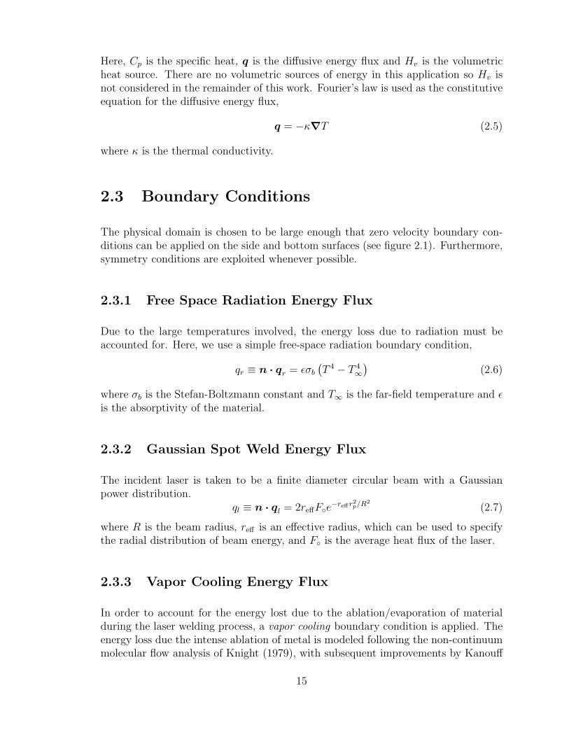
2.3.3 Vapor Cooling Energy Flux

In order to account for the energy lost due to the ablation/evaporation of materialduring the laser welding process, a vapor cooling boundary condition is applied. Theenergy loss due the intense ablation of metal is modeled following the non-continuummolecular flow analysis of Knight (1979), with subsequent improvements by Kanouff

15

0.0e+0

2.0e+8

4.0e+8

6.0e+8

8.0e+8

1.0e+9

1.2e+9

1.4e+9

1.6e+9

1.8e+9

2800 3000 3200 3400 3600

Temperature (K)

qc (

W m

-2)

Figure 2.2. The vapor cooling energy flux qc as a functionof temperature.

(2003). The resulting energy flux is fit to a piece-wise cubic polynomial which is mostconveniently expressed as a function of θ ≡ T−Tb where Tb is the boiling temperature.The function is split into three ranges of θ,

qc = n · qc =

0 : θ < 0 Kac,0 + ac,1θ + ac,2θ

2 + ac,3θ3 : 0 K < θ < 170 K

bc,0 + bc,1θ + bc,2θ2 + bc,3θ

3 : θ > 170 K.(2.8)

In this work, the coefficients in 2.8 are ac,0 = 0, ac,1 = 8.14373×105, ac,2 = −2.24831×105, ac,3 = 2.71683×101, bc,0 = −3.1036×108, bc,1 = 3.2724×106, bc,2 = −1.8084×103

and bc,3 = 2.7284 and qc has units of W ·m−2. A plot of the vapor recoil pressure asa function of temperature is given in figure 2.2.

2.3.4 Vapor Recoil Pressure Momentum Flux

In order to account for the momentum transfer due to the evaporation of materialduring the welding process, a vapor recoil pressure boundary condition is applied. Likethe vapor cooling boundary condition, this theoretical model was derived followingKnight (1979) and Kanouff (2003); the recoil pressure is specified to be a polynomialin θ ≡ T − Tb. The function is split into three ranges of θ,

pr =

0 : θ < 0 Kapr,0 + apr,1θ + apr,2θ

2 + apr,3θ3 : 0 K < θ < 170 K

bpr,0 + bpr,1θ + bpr,2θ2 + bpr,3θ

3 : θ > 170 K.(2.9)

In this work, the coefficients in 2.9 are apr,0 = 0, apr,1 = 1.851502 × 101, apr,2 =−1.969450 × 10−1, apr,3 = 1.594124 × 10−3, bpr,0 = 0, bpr,1 = −5.809553 × 101,

16

0.0e+0

2.0e+4

4.0e+4

6.0e+4

8.0e+4

1.0e+5

1.2e+5

1.4e+5

1.6e+5

1.8e+5

2.0e+5

2800 3000 3200 3400 3600

Temperature (K)

pr (

Pa

)

Figure 2.3. The vapor recoil pressure pr as a function oftemperature.

bpr,2 = 4.610515 × 10−1, and bpr,3 = 2.332819 × 10−4. The boiling temperature Tb is3000K and pr has units of Pa. A plot of the vapor recoil pressure as a function oftemperature is given in figure 2.3.

2.3.5 Free Surface Boundary Conditions

The liquid/gas interface that exists at the surface of the weld pool is free to deformin time. The dynamics of this deformation are governed in part by the vapor recoilpressure but also by the surface tension of the interface. At such an interface, thejump in normal stress across the free surface due to the presence of surface tension σis

n · (σliq − σgas) = −2Hσn−∇sσ. (2.10)

Here, −H the local mean curvature of the surface and ∇s is the surface gradientoperator, the subscripts liq and gas refer to the liquid and gas phases, respectively,and the normal vector n points from the liquid phase into the gas phase. The fullnumerical treatment of the boundary condition is well described in Cairncross et al.(2000) and will not be elaborated on here.

If one considers the gas to be a dynamically inactive and passive material then thestress vanishes in that phase except for a constant reference pressure which is typicallytaken to be zero. In that case, the stress balance in 2.10 reduces to

n · σliq = −2Hσn−∇sσ. (2.11)

17

Another observation can be made from equation 2.10. At equilibrium, the pressureis discontinuous at the free surface, viz.,

pgas − pliq = −2Hσ. (2.12)

2.4 Material Models

2.4.1 Surface Tension

The surface tension is treated as a linear function of the temperature,

σ = σ◦ − α (T − T◦) N ·m−1 (2.13)

where α is effectively dσ/dT and σ◦ is the value of the surface tension at the referencetemperature T◦.

2.4.2 Viscosity

The dynamic viscosity µ is a critical material property as was discussed in section 2.1.Here, we treat the viscosity as a piece-wise function of temperature using a fourthorder polynomial for temperatures below the liquidus temperature, TL, and a cubicpolynomial for temperatures above TL, viz.

µ =

{(cµ,0 + cµ,1TL + cµ,2T

2L + cµ,3T

3L)

[β + (1− β) T−T90

TL−T90

]: T < TL

cµ,0 + cµ,1T + cµ,2T2 + cµ,3T

3 : T ≥ TL.(2.14)

were T is max(T, Tmax) and µ has the units of Pa · s. The nominal parametersused in this study are Tmax = 4000 K, TL = 1623 K, T90 = 1528 K, β = 1011, cµ,0 =1.5616×10−1, cµ,1 = −3.3696×10−5, cµ,2 = 1.0191×10−8, and cµ,3 = −1.0413×10−12.This viscosity function is shown graphically in figure 2.4.

2.4.3 Thermal Conductivity

The thermal conductivity κ is taken to be a linear function of temperature,

κ = aκ,0 + aκ,1T W ·m−1 ·K−1 (2.15)

with aκ,0 = 10.7143 and aκ,1 = 14.2857× 10−3 and T is in Kelvin.

18

1e-1

1e+1

1e+3

1e+5

1e+7

1e+9

1e+11

1e+13

0 500 1000 1500 2000 2500

Temperature (K)

µ (

Pa s

)

TL = 1623

Figure 2.4. The viscosity µ as a function of temperature.The large values of µ at lower temperatures simulate the un-melted steel.

2.4.4 Specific Heat

The specific heat Cp is taken to be a linear function of temperature,

Cp = aCp,0 + aCp,1T J · kg−1 ·K−1 (2.16)

with aCp,0 = 425.75 and aCp,1 = 170.833× 10−3 and T is in Kelvin.

2.4.5 Density

The density ρ is taken to be a constant, ρ = 7.9× 103 kg ·m−3.

19

Chapter 3

Computational Algorithms

3.1 Interface Tracking

A key requirement in the numerical analysis of this problem is tracking the locationof the melt/air interface in time. Several methods exist for doing this numericallyand in the continuum mechanics literature these fall into two classes: conformaldiscretization and interface tracking. Naturally, each of these approaches comes withits own benefits and detriments.

Examples of conformal discretization methods include Lagrangian and ArbitraryLagrangian-Eulerian (ALE) methods. Here, the typical approach is to solve an aux-iliary system of PDEs for the unknown coordinates of the mesh points (see, e.g.,Cairncross et al. (2000)) so the mesh deforms with the material and points on theboundary of the mesh remain tied to the boundary of the material. The benefit ofthis approach is that boundary conditions can be applied in the usual way. Fields andequations always live at the same mesh points for all time so the algorithm is easyto implement. Lastly, one only needs to discretize the material of interest and notportions of space that the material may occupy at some time during the analysis. Oneproblem with conformal techniques, however, is that they tend to be computationallyexpensive. For example, a three dimensional problem may add up to three additionaldegrees of freedom at each mesh point, sometimes nearly doubling the total num-ber of degrees of freedom in the problem. A more serious problem, however, is thatsevere deformations lead to mesh entanglement and, hence, remeshing is necessary.This additional cost and complexity makes conformal interface tracking impracticalfor problems like laser welding.

Interface tracking techniques, such as level set methods (see, e.g., Sethian (1999))and volume of fluid (see, e.g., Hirt and Nicholls (1981)) take a much different ap-proach to the problem. In interface tracking methods the location of the movinginterface is typically tied to an isovalue of a scalar field. Thus, tracking the materialboundaries is more computationally efficient since one only needs to solve a scalaraxillary equation. The mesh is fixed in time and the material moves freely throughthe mesh which makes problem setup very simple and the analysis doesn’t requireremeshing no matter how complex the interface deformations are. The lack of a dis-

21

crete boundary representation for the free surface, however, means that free surfaceboundary conditions must be handled differently. Moreover, since the field discretiza-tions are non-conformal with the free boundary, it’s not always possible to specify theboundary conditions accurately. Though it’s not a requirement of interface trackingtechniques, many implementations require all fields and equations to be defined overthe entire mesh and that their values be computed at all times. This causes additionalcomputational expense and, often times, computational difficulty due to scaling andresolution problems.

3.2 The Level Set Method

Due to the computational efficiency and the easy of use, our work here focuses onusing the level set method for tracking the free surface. However, ALE simulationsfor problems with mild deformations are used as a means of assessing the accuracyof the level set simulations. In this section, we provide the details of the level setalgorithm as it is implemented in Aria and used in this work.

First, we define a signed distance function F (x, t) that is a function of space x andtime t and whose magnitude is the shortest distance from x to any point on the freesurface, viz. the contour F = 0 defines the free boundary tracked by F . The signof F is used to indicate whether the point x lies inside the material. Notationally,we denote these two sides of the interface as “phase A” and “phase B” and often use“A” and “B” as subscripts on mathematical quantities that are specific to a phase.Lastly, by convention, we associate phase A with F < 0.

In order to perform integrations over each phase, it’s convenient to introduce a Heav-iside function Hi(F ) which is unity in phase i and zero in the other phase. Moreover,HA and HB are related as HB = 1 − HA. In so-called diffuse interface approaches,the Heaviside function is regularized so that there is a smooth transition from onephase to another. In this work, we use

HB(F ) =

0 : F < −α

212

[1 + F

α/2+ 1

πsin

(π F

α/2

)]: −α

2< F < α

2

1 : F > α2

(3.1)

where α is defined as the width of the interfacial region. Likewise, one can define aregularized delta function as,

δ(F ) =dH(F )

dF=

0 : F < −α

2|∇F |

α

[1 + cos

(π F

α/2

)]:

: −α2

< F < α2

0 : F > α2

(3.2)

Figure 3.1 illustrates HB(F ) and δ(F ) for the case of α = 1.

22

-0.2

0.0

0.2

0.4

0.6

0.8

1.0

1.2

1.4

1.6

1.8

2.0

2.2

-1.5 -1.0 -0.5 0.0 0.5 1.0 1.5

F

HB, !

"

HB(F)

!(F)

Figure 3.1. A plot of the regularized Heaviside (Eq. 3.1)and delta (Eq. 3.2) functions for an interfacial width α = 1.

The distance function F must evolve in time as a part of the simulation in order totrack the free surface location. Depending on the physics involved in a problem theremay be different conditions which can be used to evolve the free surface in time. Forexample, in a phase change problem, the net normal flux of mass may define theinterfacial velocity and hence its motion. In two phase flow problems, such as thelaser welding application under study in this work, F is typically evolved using atransport equation,

∂F

∂t+ ve · ∇F = 0 (3.3)

where ve is the so-called extension velocity. The extension velocity is a vector fielddefined as the velocity which preserves the distance quality of F . Unfortunately, thisfield is not known and, in general, may be multi-valued or singular at some points inspace and time. The typical approach is to instead use the fluid velocity v,

∂F

∂t+ v · ∇F = 0. (3.4)

A consequence of this compromise is that distance quality of F will degrade in timeand so redistancing or renormalizing algorithms must be run periodically to correctF . In this work, we utilize a constrained redistancing algorithm that attempts toredistance F so that the volume of each phase remains unchanged.

Note that equation 3.4 is purely hyperbolic. With the initialization of F and condi-tion that the free surface defines the F = 0 isosurface, boundary conditions are notrequired.

23

3.3 ALE Mesh Motion

As described above, conformal moving-mesh algorithms have distinct advantages thatmake them ideal for verifying the accuracy of level set simulations. Furthermore, sinceAria has both ALE and level set capabilities we will use ALE simulations as the basisfor assessing the performance and accuracy of the more generally applicable level setsimulations.

The ALE approach used in Aria is the pseudo-solid approach described by Cairncrosset al. (2000). Here, the mesh is treated as though the nodes were material points of asolid that deforms quasi-statically. In Aria, we use a hyperelastic material descriptionwhere the material coordinates X in the undeformed reference frame are related tothe physical coordinates x in the physical reference frame by a displacement field d,viz.,

x = X + d (3.5)

In this case, the Cauchy momentum equation that governs the quasi-static deforma-tion of this pseudo-solid reduces to

∇ · σm = 0 (3.6)

where σm is the mesh (solid) stress tensor. Due to the large deformations that canoccur we choose here to use a nonlinear neo-Hookean elastic constitutive equation.First, it’s convenient to define the deformation gradient F ,

F ≡ ∇Xxt

= ∇XX t + ∇Xdt

= I + ∇Xdt

where ∇X is the gradient operator in the undeformed reference frame. Then, theneo-Hookean elastic constitutive equation can be written as

σm =µ

J(b− I) +

λ

Jln JI (3.7)

where λ and µ and the Lame coefficients, b ≡ F · F t is the left Cauchy-Green tensorand J ≡ det F . See, e.g., Bonet and Wood (1997) or Belytschko et al. (2004).

The boundary conditions on the mesh equation are very straight forward. On externalboundaries, we prohibit normal displacements, n · d = 0, but leave the mesh pointsfree to move tangentially in order to minimize mesh distortions. Along the freesurface, we use the kinematic boundary condition,

n ·(

dd

dt− v

)= 0 (3.8)

which states that material points on the surface remain on the surface.

24

3.4 The Finite Element Method

The system of equations to be solved include the conservation equations 2.1, 2.3 and2.4 and the axillary equations for either interface tracking 3.4 or the mesh displace-ments 3.6. Respectively, the unknown fields in the problem are the velocity v, pressurep, temperature T and either the distance function F or the mesh displacements d.We solve this system of equations, subject to the boundary and initial conditionsoutlined above, using the Galerkin finite element method (G/FEM). G/FEM is awell established method for solving boundary value problems so we only describe itbriefly here; full details of the method are available in Hughes (2000).

Each unknown field X is discretize by defining a set of basis functions {φX} andcoefficients {X} such that,

X(x, t) =

NX∑i=1

Xi(t)φiX(x) (3.9)

where NX is the number of basis functions and coefficients in the discretization. Thebasis functions {φX} are selected to be low order polynomials with local support.

Weak residuals of the governing PDEs are formed using the basis functions as theweighting functions. The residual form for the governing PDEs are summarized inequations 3.10–3.14.

Rim,k =

∫V

[(ρ∂v

∂t+ ρv · ∇v − ρg

)· ekφ

i + σt : ∇(ekφ

i)]

dV −∫S

n · σ · ekφi dS = 0

(3.10)

RiP = −

∫V

∇ · vφi dV = 0 (3.11)

RiT =

∫V

[(ρCp

∂T

∂t+ ρCpv · ∇T

)φi −∇φi · q

]dV +

∫S

n · qφi dS = 0 (3.12)

RiF =

∫V

(∂F

∂t+ v · ∇F

)φi dV = 0 (3.13)

Rim,k =

∫V

σtm : ∇

(ekφ

i)

dV = 0 (3.14)

Time derivatives are discretized using a first-order finite-difference (Euler) approxi-mation. We use an explicit forward Euler approximation for the first four time stepsfollowed by an implicit backward Euler approximation for subsequent time steps.

With this discretization in place, what remains is a large system of discrete nonlinearequations. This system is solved using Newton’s method with analytic sensitivitiesfor the Jacobian matrix.

25

3.5 Pressure Stabilization

For the finite element solution of the Navier-Stokes equations, there exist mathemat-ical restrictions on the choice of basis functions for the velocity and pressure degreesof freedom. The details of this restriction are beyond the scope of this report butmay be found elsewhere (see, e.g., Hughes 2000). In order to obtain solutions to theproblem, one must either use a compatible pair of finite element basis functions or addstabilization terms to relieve the mathematical restrictions. For the sake of computa-tional efficiency and geometric accuracy for the level set algorithms we prefer to uselinear, nodal, C0-continuous basis functions for all of our unknown fields. However,in order to do so we must employ some form of velocity-pressure stabilization.

Here, we employ the stabilization technique developed by Dohrmann and Bochev(2004). In addition to being computationally efficient and easy to implement, thisstabilization method is also easy to use since it requires no special treatment forboundary conditions. Numerically, this method simply requires an additional volumeintegral term in the weak form of the continuity equation (equation 3.11).

3.6 Adaptive Mesh Refinement

A key to obtaining accurate simulation results with level set methods is sufficientresolution of the interfacial region. Since the interface typically propagates throughthe mesh in time, the mesh needs to have sufficiently small elements where ever theinterface may pass. This worst-case approach to mesh refinement can lead to verycomputationally expensive simulations, especially in 3D. A remedy to this problemis to use adaptive mesh refinement (AMR) or h-adaptivity. The Aria application isbuilt on top of the SIERRA framework (Edwards 2002) and so inherits an adaptivemesh refinement capability (Steward and Edwards 2002). The AMR capability allowssome of the elements in a mesh to be refined (subdivided) and later unrefined to asto produce a locally refined mesh.

There are a two basic elements that contribute to the overall AMR algorithm in Aria.The first is that elements are marked for refinement according to some criterion thatthe user specifies. This step includes imposing a 2:1 refinement constraint so thatan element’s neighboring elements are never split more than once (see Steward andEdwards 2002). The second step is the actual refinement or unrefinement of elements.This step includes the prolongation of the unknown fields to new nodes in the meshand the addition of hanging node constraints to the linear system to account for anynonconformal element boundaries. In order to use AMR an analyst only needs tospecify a element marking function.

In this work, we use an element marking function that ensures that elements withina specified distance of the F = 0 interface have a size that is smaller than a specified

26

length scale. Since the interfacial width α is already supplied as part of the levelset algorithm, it’s convenient then to specify the desired number of elements acrossthis width, nα, so that the element length-scale in the interfacial region will be hI ≡α/nα. In order to avoid excessive refinement and unrefinement at each time step,this marking criterion is applied to all elements where |F | < α/2+ 3

2hI at some point

within the element.

It is important to note that the accuracy and efficiency of the level set algorithm isheavily dependent on the parameters α and nα. If either α or nα is too large thenthe diffusive nature of the level set algorithm can lead to significant losses of mass,momentum and energy. Also, if α/nα is too large then the interfacial contributionsto 3.10–3.14 will be under-resolved and, again, lead to inaccuracies. Lastly, if nα islarge the problem becomes very computationally expensive. Experience has lead to arecommended value of nα = 4. Recommended values of α, however, are very problemdependent. In this work, α is most closely correlated with the radius of the laser andis usually on the order of 10% of the beam radius.

27

Chapter 4

Results

4.1 Comparisons Between Goma and Aria Weld

Simulations

Verification of the weld model implementation in Aria was accomplished by compari-son with the Goma weld model results for a 2D spot weld. For the sake of simplicity,surface deformations were ignored for this simulation. Figure 4.1 shows the weldpool, velocity vectors, and temperature distribution after a 1 ms 200 W laser pulse,with a 0.1 mm spot radius. This power level produces a bowl-shaped melt pool withcounter-rotating convection cells driving surface flows from the center of weld to theedges. The flow direction is determined by the temperature-dependent surface ten-sion, which generally decreases with temperature for most metals. The contour marksthe liquidus temperature.

Figures 4.2 and 4.3 compare the shear velocity on the weld pool surface and surfacetemperature between Goma and Aria simulations. The close comparison verifies themodel implementation in Aria, especially given the complexity of the physics beingmodeled.

4.2 Comparisons with Spot Weld Experiments

Experiments on spot welds performed by J. Norris and C Robino (SNL, Joining andCoating Department, 1813) provide an opportunity for validation of the Aria weldmodel. The set of experiments considered here involve a 3.3 J/6 ms laser powersetting, with a 350 micron beam radius on 304L stainless steel. The welds wereperformed using several different shield gases, including argon, nitrogen and air. Theshield gas has a profound effect on the weld profile, depending of whether it providesan inert (argon) or oxidizing (air) atmosphere.

Figures 4.4 and 4.5 compare the weld profiles using argon and air as the shield gases,respectively. These are results from two-dimensional simulations whereas the weldsare axisymmetric at this laser power. The experimental weld pool profiles are shown

29

Figure 4.1. Weld pool shape and temperature distribution(2D) at 1 ms in stainless steel SS304L.

Figure 4.2. Comparison of surface shear velocity compo-nents at 1 ms for a 2D spot weld simulation.

30

Figure 4.3. Comparison of surface temperature profile at1 ms for a 2D spot weld simulation.

in red and the computed temperature contours in black. The color fringe depicts thetemperature distribution as 6 ms. Also shown are instantaneous streamlines. Theshield gas has a profound effect on the weld profiles. The surface tension of metalsgenerally decreases with temperature. However, it is well known that dissolution ofimpurities, as might be introduced by oxidation, profoundly change the character ofsurface tension, generally significantly reducing the value near the melt point andincreasing with temperature thereafter. In the simulations, with argon as the shieldgas, the surface tension specified represents pure Fe. In this case the convectivecirculation on the surface is from the center towards the edges. This pattern bringshot molten metal to the periphery of the weld, which in the simulations promotesthe lateral melting of the metal, resulting in a shallow weld pool. In the figure, thecirculation exists only at the edges of the weld, while the central portion is largelyquiescent. The absorptivity was set at 25%, resulting in a width/depth of 734/152microns, compared with 675/270 in the experiments.

With air as shield gas the surface tension was modeled after the idealized gradient usedin Tanaka and Lowke (2007) for SUS 304 with high sulfur concentration (σ◦ = 1.36N/m; α = −2.1 × 10−4 N/m/K; see equation 2.13. Here the flow on the surface isfrom the edges of the weld pool towards the center, resulting in a downward directedjet of molten metal in the central portion of the weld pool. The positive surfacetension gradient results in deeper welds because the circulation convects hot moltenmetal downward towards the bottom of the weld pool.

Using a fixed absorptivity of 30%, the figure shows reasonably good comparison withthe experimental profile. The computations result in a width/depth of 640/261 (mi-crons) compared to the experimental values of 675/270.

31

500 micron

Figure 4.4. Weld profiles in stainless steel SS304L with Ar-gon as shield gas. The profile in red is from the experimentswhich is compared to the temperature profiles in black. Thecoolest isotherm depicts liquidus.

32

500 micron

Figure 4.5. Weld profiles in stainless steel SS304L withair as shield gas. The profile in red is from the experimentswhich is compared to the temperature profiles in black. Thecoolest isotherm depicts liquidus.

33

4.3 Comparisons Between ALE and Level Set Al-

gorithms

As noted in chapter 3 there are distinct advantages for both the ALE (conformalmesh) and level set (interface tracking) algorithms for simulating free surface flows.The level set algorithm is desirable because of its ease of use and its ability to capturelarge deformations and topological changes in deforming media. In this section wemake comparisons between level set simulations and ALE simulations.

4.3.1 Effect of Including the Gas Phase

When the gas phase above the weld pool free surface is included in the simulationthe pressure and velocity fields are treated as continuous between the two phases.Due to the presence of the gas, the stress balance at the free surface includes thestresses from the air phase. As discussed in section 2.3.5, the pressure is actuallydiscontinuous at the free surface, in proportion to the surface tension and curvatureof the free surface,

pgas − pliq = −2Hσ. (4.1)

Equation 4.1 makes clear that in the presence of surface tension, the pressure isdiscontinuous at the interface. However, in the current level set algorithm all fields,including the pressure, are continuous across the interface. The result of this pressurecontinuity is that an artificial pressure gradient normal to the interface exists andleads to a mass flux across the interface. This effect can be seen by comparing threeALE simulations. In the first simulation, illustrated in figure 4.6, the gas phase isnot simulated and so there is no artificial pressure gradient at the free surface and somass is conserved; the volume of fluid displaced from the weld pool accumulates in abulging ring around the edge of the weld.

In the second ALE simulation, illustrated in figure 4.7, we include the ambient gasphase which results in a mass loss in the liquid phase due to the artificial pressuregradient at the interface.

In the final ALE simulation, we include the gas phase in the simulation but use twodifferent pressure fields, one for each phase, so that the pressure is discontinuousacross the gas/liquid interface. In this case, figure 4.8, volume is again conservedsince there is no artificial pressure gradient at the interface.

The level set algorithm currently available in Aria does not support discontinuousfields across the interface. Accordingly, this mass loss effect is observed for level setsimulations. However, the amount of artificial mass transfer is proportional to thevolume of the elements along the free surface (where the gradient exists). Thus, usinga finer mesh or adaptive mesh refinement can reduce this effect. Using the adaptive

34

Figure 4.6. Weld pool shape and temperature profile for a3D ALE simulation.

Figure 4.7. Weld pool shape and temperature profile for a3D ALE simulation with the ambient air phase simulated.

35

Figure 4.8. Weld pool shape and temperature profile fora 3D ALE simulation with the ambient air phase simulated.Here, the pressure is allowed to be discontinuous at the liq-uid/gas interface.

mesh refinement capabilities in Aria, the mesh is adapted dynamically to achieve aspecified element length scale in the interface region. In figures 4.9–4.11 we keepthe number of elements across the interfacial region nα (see section 3.6) constantbut reduce the interfacial thickness α. The result is that as α decreases so does theelement length scale at the interface, hI ≡ α/nα.

Figure 4.12 quantifies the reduced mass loss of the liquid phase for both ALE andlevel set (LS) simulations. Here, the course mesh ALE simulation with continuouspressure demonstrates the most sever loss of mass where as the ALE simulation whichaccommodates the pressure discontinuity provides a near exact conservation of mass.The level set simulations demonstrate that as the element length scale at the freesurface approaches zero, the mass conservation improves. Advancing the level setalgorithm to accommodate a discontinuous pressure is part of the ongoing work inAria.

4.4 Demonstration Calculation: 3D Line Weld

In this section we simply report a demonstration calculation of a traveling line weld.In this case, the laser heat flux boundary condition in equation 2.7 was extendedto allow a prescribed motion of the laser source. Figure 4.13 shows the free surfaceposition and temperature distribution for such a weld. Likewise, figure 4.14 shows

36

Figure 4.9. Weld pool shape and temperature profile fora 3D level set simulation with α = 4 × 105, nα = 4 andhI = 1× 10−5.

Figure 4.10. Weld pool shape and temperature profile fora 3D level set simulation with α = 2 × 105, nα = 4 andhI = 0.5× 10−5.

37

Figure 4.11. Weld pool shape and temperature profile fora 3D level set simulation with α = 1 × 105, nα = 4 andhI = 0.25× 10−5.

6.05e-11

6.06e-11

6.07e-11

6.08e-11

6.09e-11

6.10e-11

6.11e-11

6.12e-11

6.13e-11

0.0e+00 2.0e-04 4.0e-04 6.0e-04 8.0e-04 1.0e-03

Time (s)

Vli

q (

m3)

ALE with Discontinuous Pressure

ALE with Continuous Pressure

LS, hI = 0.25 x 10-5 m

LS, hI = 0.5 x 10-5 m

LS, hI = 1 x 10-5 m

Figure 4.12. Volume of the liquid (metal) phase as a func-tion of time as predicted by the ALE and level set (LS) sim-ulations. Physically, the volume of this phase should be con-stant for all times. These results illustrate the fictitious massloss over time due to a continuous pressure for both ALE andLS simulation with varying interfacial elements sizes.

38

the corresponding ALE simulation which shows excellent agreement with the level setresults.

39

Figure 4.13. Temperature distributions and weld poolshapes at three instances during a moving line weld usingthe level set algorithm.

40

Figure 4.14. Temperature distributions and weld poolshapes at three instances during a moving line weld usingthe ALE algorithm.

41

Chapter 5

Recommendations for Future Work

In this chapter we lay forth recommendations and lessons learned during the com-pletion of this Milestone. We make suggestions to analysts who intend to do studiessimilar to the work undertaken here. We also outline some future development activ-ities that could lead to a more accurate, robust and efficient tool for problems suchas laser welding.

5.1 Linear Tetrahedral Elements are Preferred

The foundational algorithms within the level set capability rely on the accurate repre-sentation and manipulation of geometric primitives such as quadrilaterals, triangles,hexahedron and tetrahedron. Two critical requirements are that these algorithms (a)remain true to the original problem discretization and (b) are convergent with meshrefinement. In cases where these two requirements are at odds with one another wechoose the first. However, these two requirements can be achieved when the originalmesh discretization is restricted to linear tetrahedral elements. Higher order tetra-hedral basis functions can be used if the element geometries are restricted to linear(planer surfaces).

5.2 Adaptivity is Essential for Efficiency and Ac-

curacy

As discussed in section 3.6 adaptivity is a key capability for the successful deploymentof level set algorithms for large scale, 3D, free-surface flows with significant surfacetension effects. Adaptivity, when combined with linear tetrahedral elements, enablesthe most efficient and accurate simulations for the current generation of level setalgorithms available in Aria. Future algorithms may alleviate the need for adaptivitybut that appears unlikely.

43

5.3 Support for Discontinuous Fields at Interfaces

In section 4.3.1 we described the inaccuracies that arise when the pressure is con-strained to be continuous across the free surface. The ability to capture the correctpressure jump at the interface would lead to more accurate results. Moreover, thenumerical artifacts often lead to spurious currents in the flow field. These numericalartifacts can cause the time integration algorithms to operate with a much smallertime step size than would otherwise be necessary and, thereby, increase the overallcomputational cost of a simulation.

5.4 Improved Level Set Performance

The current implementation of the level set capability in Aria could benefit from per-formance enhancements. Despite the efficiencies gained from utilizing the adaptivemesh refinement capability, accurate simulations still require a large number of de-grees of freedom compared to the ALE algorithm. Adding support for discontinuouspressures at a free surface should help alleviate the problem. Sharp integration of levelset surfaces could also reduce the number of degrees of freedom required for accuratesolutions. Additional gains could be made from removing the gas phase entirely fromthe simulation for problems, such as laser welding, where the details there are ofno interest. Lastly, the entire algorithm should be profiled for inefficiencies; coursegrained timing diagnostics currently available suggest there may be inefficiencies atthe interface with the linear solver.

44

Appendix A

Example input Files

This appendix contains representative input files for performing the level set simula-tions of a stationary, 3D spot weld with Aria. Section A.1 contains the Cubit input(“journal”) file for generating the input mesh to be used by Aria. Section A.2 containsthe Aria input file for the simulation. Full details about the parameters and modeldetails for the Aria input file can be found in the Aria User Manual (Notz et al. 2007).

A.1 Cubit Journal File

# SCALE = {SCALE = 0.001}

# LX = {LX = 0.7}

# LY = {LY = 0.7}

# LZ_BOT = {LZ_BOT = 0.5}

# LZ_TOP = {LZ_TOP = 0.1}

reset

set associativity complete on

create brick width {LX/2} depth {LY/2} height {LZ_BOT}

body 1 move {LX/4} {LY/4} {-LZ_BOT/2}

create brick width {LX/2} depth {LY/2} height {LZ_TOP}

body 2 move {LX/4} {LY/4} {LZ_TOP/2}

merge all

#curve all interval 15

#curve 3 interval 30



surface 1 size {0.01*2*0.7}

surfa all scheme trimesh

mesh surface 1

45

surface 3 sizing function type bias start curve 4 factor 1.1








mesh surface 3 4 5 6 9 10 11 12

sideset 1 surface 4 10 # x = xmin

sideset 2 surface 6 12 # x = xmax

sideset 3 surface 3 9 # y = ymin

sideset 4 surface 5 11 # y = ymax

sideset 5 surface 2 # z = zmin

sideset 6 surface 7 # z = zmax

volume all scheme tetmesh

mesh volume all

merge all

block 1 volume 1 2

transform mesh output scale {SCALE}

export genesis "spot3d_quarter_graded_mesh_T1.exoII" overwrite

A.2 Aria Input File

#

# alpha = {alpha=2.e-5}

# beam_radius = {beam_radius = 0.0001}

# elem_per_alpha = {elem_per_alpha = 4}

#

Begin Sierra 3D_ALE_Laser_Spot-Welding_Test

Begin Aria Material multiphase

Level Set Heaviside = Smooth

Level Set Width = Constant width={alpha}

Surface Tension = Linear_T sigma0= 1.943 dsigmadT=-4.3e-4 T_ref=1809

thermal conductivity = Phase_Average

Viscosity = Phase_Average

46

End

Begin Aria Material Stainless # Units in mks

Density = Constant Rho = 7900.

Viscosity = Weld c0=0.15616 c1=-3.3696e-5 c2=1.0191e-8 \$

c3=-1.0413e-12 T_liq=1623 T_90=1528 T_max=4000

Specific Heat = Polynomial Variable=Temperature Order=1 C0=425.75 \$

C1=170.833e-3

Thermal Conductivity = Thermal A =10.7143 B=14.2857e-3 C=0 D=0

Momentum Stress = Incompressible_Newtonian

Momentum Stress = LS_Capillary

Heat Conduction = Fouriers_Law

End

Begin Aria Material air

Density = Constant Rho = 1

Viscosity = Constant mu = {2.e-5 * 1000}

Thermal Conductivity = Constant K = 0.025

Specific Heat = Constant Cp = 1000

Momentum Stress = Incompressible_Newtonian

Momentum Stress = LS_Capillary

Heat Conduction = Fouriers_Law

End

Begin Aztec Equation Solver gmres_ilut

solution method = gmres

preconditioning method = dd-ilut

maximum iterations = 500

param-int AZ_kspace value 500

residual norm tolerance = 1.e-6

param-real AZ_drop value 1e-8

param-int AZ_ilut_fill value 2

preconditioner subdomain overlap = 2

matrix reduction = fei-remove-slaves

End

Begin Finite Element Model The_Model

Database Name = spot3d_quarter_graded_mesh_T1.exoII

Begin Parameters For Block block_1

material multiphase

phase a = stainless

phase b = air

End

End

47

Begin Adaptivity Controller my_adaptive_strategy

Max Outer Adapt Steps is 1

Max Inner Adapt Steps is 1

End

Begin Zoltan Parameters Zoltan_Params

Load Balancing Method = Hilbert Space Filling Curve

Over Allocate Memory = 1.5

Reuse Cuts = true

Algorithm Debug Level = 2

Check Geometry = true

Zoltan Debug Level = 2

Timer = cpu

Debug Memory = 0

End

Begin Procedure The_Procedure

Begin Solution Control Description

Use System Main

Begin System Main

Simulation Start Time = 0.000

Simulation Termination Time = 0.001

Simulation Max Global Iterations = 2000

Begin Transient The_Time_Block

Advance The_Region

Event LS_CONSTRAINED_REDISTANCE when "(CURRENT_STEP - \$

LAST_LS_CONSTRAINED_REDISTANCE_STEP) >= 25 || \$

(LS_GRADIENT_ERROR_NORM(0.) > 0.1 && (CURRENT_STEP - \$

LAST_LS_CONSTRAINED_REDISTANCE_STEP) >= 5)"

Event LS_COMPUTE_SIZES

End

End

Begin Parameters For Transient The_Time_Block

Start Time = 0.0

Begin Parameters For Aria Region The_Region

Initial Time Step Size = 1.e-6

Maximum Time Step Size = 5.e-6

Minimum Time Step Size = 1.e-9

Minimum Resolved Time Step Size = 1.e-8

Time Step Variation = Adaptive

Predictor-Corrector Tolerance = 0.01

Courant Limit = 0.5

End

48

End

End

Begin Aria Region The_Region

Use Finite Element Model The_Model

Use Adaptivity Controller my_adaptive_strategy

Adapt Mesh on Isovolume Level_Set h={h=alpha/elem_per_alpha} \$

min={-(alpha/2+1.5*h)} max={alpha/2+1.5*h}

Enable Rebalance with Threshold = 1.2 Using Zoltan Parameters \$

Zoltan_Params

Rebalance Load Measure Type = Constant

Use Linear Solver gmres_ilut

Predictor Fields = Velocity

Predictor Fields = Temperature

Predictor Fields = Not Pressure

Nonlinear Solution Strategy = Newton

Maximum Nonlinear Iterations = 10

Nonlinear Residual Tolerance = 1.0e-6

Nonlinear Relaxation Factor = 1.0

nonlinear correction tolerance = 0

EQ Level_Set for Level_Set on block_1 Using Q1 with Mass Adv

IC Linear on block_1 Level_Set COEFF = 0.0 0.0 0.0 1.0

Advection Velocity for Level_Set = OLD_VELOCITY

Begin Level Set Interface LS

Distance Variable = solution->LEVEL_SET

Velocity Variable = solution->VELOCITY

Narrow Band Width = {4.0*alpha}

EnD

EQ Momentum_A For Velocity On block_1 Using Q1 With Mass Adv Diff Src

EQ Momentum_B For Velocity On block_1 Using Q1 With Mass Adv Diff Src

Pressure Stabilization Is PSPP_CONSTANT With Scaling = 1.0

EQ Continuity_A For Pressure On block_1 Using Q1 With Div

EQ Continuity_B For Pressure On block_1 Using Q1 With Div

BC Const Dirichlet At surface_1 Velocity_X = 0.0

49


BC Const Dirichlet At surface_2 Velocity_Y = 0.0

BC Const Dirichlet At surface_2 Velocity_Z = 0.0








Source For Momentum_A On block_1 = Hydrostatic gx=0.0 gy=0.0 gz=-9.81

Source For Momentum_B On block_1 = Hydrostatic gx=0.0 gy=0.0 gz=-9.81

EQ Energy_A for Temperature on block_1 using Q1 with Mass Adv Diff

EQ Energy_B for Temperature on block_1 using Q1 with Mass Adv Diff

IC Const on block_1 Temperature = 300.

BC Const Dirichlet on surface_5 Temperature = 300.

BC Diffuse for Momentum_A on surface_AB = Vapor_Recoil_Pressure \$

TBOIL = 3000.

BC Diffuse for Momentum_B on surface_AB = Vapor_Recoil_Pressure \$

TBOIL = 3000.

BC Diffuse for Energy_A on surface_AB = Gaussian_Spot_Weld src_x=0 \$

src_y=0 src_z=1 dir_x=0 dir_y=0 dir_z=-1 R={beam_radius} \$

Flux = 2.546e9 R_EFF = 0.6

BC Diffuse for Energy_B on surface_AB = Gaussian_Spot_Weld src_x=0 \$

src_y=0 src_z=1 dir_x=0 dir_y=0 dir_z=-1 R={beam_radius} \$

Flux = 2.546e9 R_EFF = 0.6

BC Diffuse for Energy_A on surface_AB = Rad TO=300 CRAD=5.67e-8

BC Diffuse for Energy_B on surface_AB = Rad TO=300 CRAD=5.67e-8

BC Diffuse for Energy_A on surface_AB = Vapor_Cooling Tboil=3000.

BC Diffuse for Energy_B on surface_AB = Vapor_Cooling Tboil=3000.

Postprocess Viscosity on block_1

Postprocess thermal_conductivity on block_1

Begin Results Output The_Output

Database Name = soln.e

At Step 0, Increment is 10

Title Spot Weld

50

Nodal Variables = solution->Level_Set as F

Nodal Variables = solution->Velocity as V

Nodal Variables = solution->Pressure as P

Nodal Variables = solution->Temperature as T

Nodal Variables = pp->Viscosity as MU

Nodal Variables = pp->thermal_conductivity as K

End

End

End

End

51

References

Ted Belytschko, Wing Kam Liu, and Brian Moran. Nonlinear Finite Elements forContinua and Structures. John Wiley and Sons, 2004. 3.3

Javier Bonet and Richard D. Wood. Nonlinear Continuum Mechanics for FiniteElement Analysis. Cambridge University Press, 1997. 3.3

R. A. Cairncross, P. R. Schunk, T. A. Baer, R. R. Rao, and P. A. Sackinger. A finiteelement method for free surface flows of incompressible fluids in three dimensions.part i. boundary fitted mesh motion. Int. J. Numer. Methd. Fluids, 33:375–403,2000. 2.3.5, 3.1, 3.3

Clark R. Dohrmann and Pavel B. Bochev. A stabilized finite element method forthe Stokes problem based on polynomial pressure projections. Int. J. Num. Meth.Fluids, 46:183–201, 2004. 3.5

H. C. Edwards. SIERRA Framework version 3: core theory and design. TechnicalReport SAND2002-3616, Sandia National Laboratories, 2002. 3.6

C. W. Hirt and B. D. Nicholls. Volume of fluid (VOF) method for dynamics of freeboundaries. J. Comp. Phys., 39:201–225, 1981. 3.1

T. J. R. Hughes. The Finite Element Method. Dover Publications, New York, USA,2000. 3.4, 3.5

M. P. Kanouff. Vapor recoil pressure II. Technical Report Internal Memorandum,Sandia National Laboratories, Albuquerque, NM, USA, March 2003. 2.3.3, 2.3.4

C. J. Knight. Theoretical modeling of rapid surface vaporization with back pressure.AIAA Journal, 17(5):519–523, 1979. 2.3.3, 2.3.4

P. K. Notz, S. R. Subia, M. M. Hopkins, H. K. Moffat, and D. R. Noble. Aria 1.6user manual. In preparation, 2007. A

J. A. Sethian. Level Set Methods and Fast Marching Methods, volume 3 of CambridgeMonographs on Applied and Computational Mathematics. Cambridge UniversityPress, New York, USA, 2nd edition, 1999. 3.1

J. R. Steward and H. C. Edwards. SIERRA Framework version 3: h-adaptivity designand use. Technical Report SAND2002-4016, Sandia National Laboratories, 2002.3.6

M. Tanaka and J. J. Lowke. Predictions of weld pool profiles using plasma physics.J. Phys. D: Appl. Phys., 40:R1–R23, 2007. 4.2

53

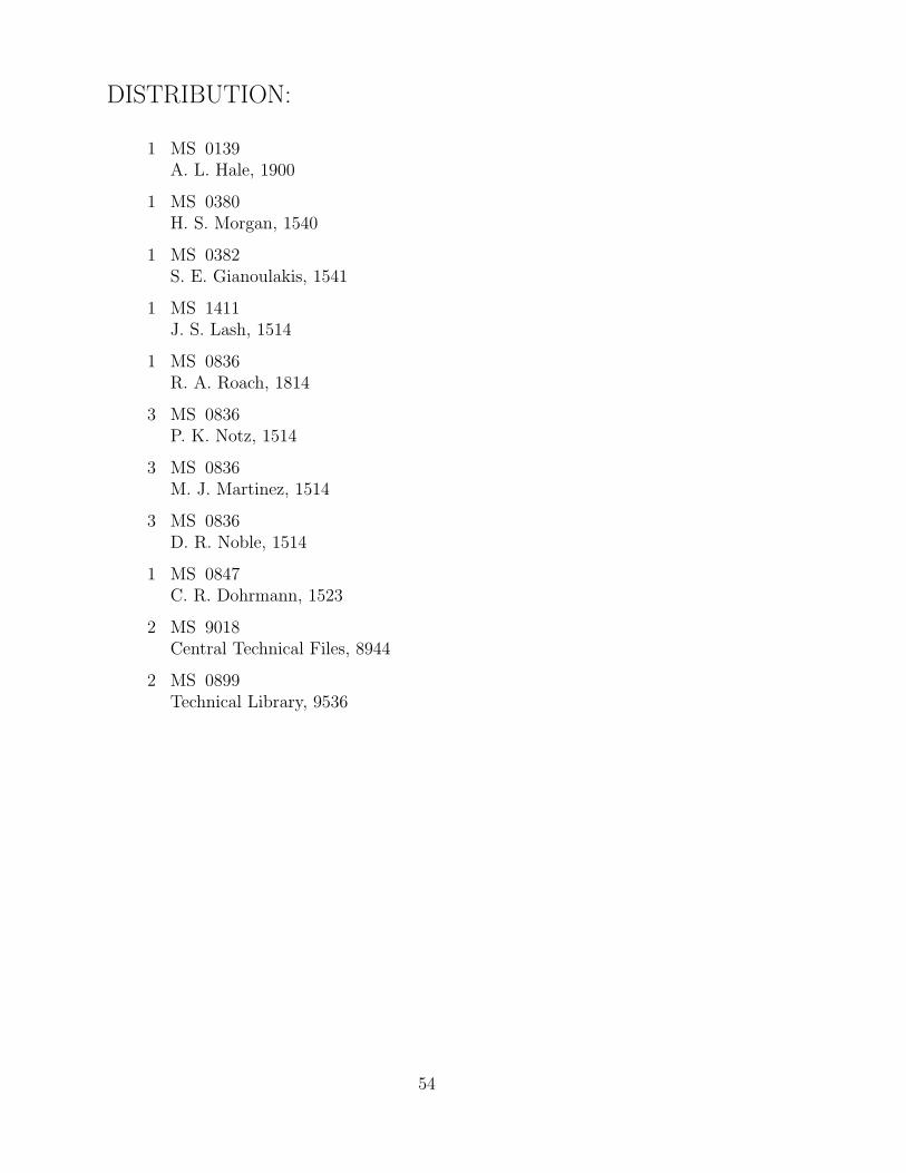
DISTRIBUTION:

1 MS 0139A. L. Hale, 1900

1 MS 0380H. S. Morgan, 1540

1 MS 0382S. E. Gianoulakis, 1541

1 MS 1411J. S. Lash, 1514

1 MS 0836R. A. Roach, 1814

3 MS 0836P. K. Notz, 1514

3 MS 0836M. J. Martinez, 1514

3 MS 0836D. R. Noble, 1514

1 MS 0847C. R. Dohrmann, 1523

2 MS 9018Central Technical Files, 8944

2 MS 0899Technical Library, 9536

54

use of aria to simulate laser weld pool dynamics for...

Documents