1

Use of Benchmark Concentration Modeling and Categorical Regression

to Evaluate the Effects of Acute Exposure

To Chloropicrin Vapor Part I. Technical Report

Prepared for:

The Chloropicrin Manufacturer’s Task Force

Prepared by:

Toxicology Excellence for Risk Assessment (TERA)

July 6, 2005

The opinions expressed in this text are those of the authors and do not necessarily represent the views of the sponsors.

2

Table of Contents List of Tables .................................................................................................................................. 3 List of Figures ................................................................................................................................. 4 1.0 EXECUTIVE SUMMARY ...................................................................................................... 5 2.0 OVERVIEW ............................................................................................................................. 7 3.0 BACKGROUND FOR BMC .................................................................................................... 7 4.0 BACKGROUND FOR CATEGORICAL REGRESSION ....................................................... 8 5.0 CATEGORIZATION OF DATA ........................................................................................... 10

5.1 Categorization Approach - Phase 1 of Cain Study ............................................................. 11 5.2 Categorization Approach - Phase 2 of Cain Study ............................................................. 11 5.3 Categorization Approach - Phase 3 of Cain Study ............................................................. 12 5.4 Categorization of Animal Data ........................................................................................... 15

6.0 BMC MODELING APPROACH ........................................................................................... 17

6.1 Continuous Data Modeling ................................................................................................. 17 6.2 Quantal Data Modeling ....................................................................................................... 18

7.0 RESULTS ............................................................................................................................... 19

7.1 Benchmark Concentrations ................................................................................................. 19 7.2 Graphical Presentation of Group-Level Severity ................................................................ 23 7.3 Categorical Regression Results .......................................................................................... 25

8.0 DERIVATION OF EXPOSURE LIMITS .............................................................................. 34 9.0 REFERENCES ....................................................................................................................... 40 10.0 BIOS OF KEY AUTHORS .................................................................................................. 42

3

List of Tables Table 1. Ocular Symptom Incidence Calculated for Use in BMC Modeling .............................. 19 Table 2. Benchmark Concentrations for Nasal NO ..................................................................... 20 Table 3. Benchmark Concentrations Calculated for Ocular Symptoms ...................................... 21 Table 4. Summary of Benchmark Modeling Results for Cain (2004) ......................................... 22 Table 5. Holistic Evaluation of % Responding for Cain (2004) (Results of Two Independent Evaluations) .................................................................................................................................. 23 Table 6. Summary Statistics for the Categorical Regressions Using the Data Set of Choice, Cumulative Odds Model ............................................................................................................... 27 Table 7. Summary of Human EC10 Results for Model of Choice SEV1: AEL1 ........................ 34 Table 8. Summary of Exposure Limit Derivation ....................................................................... 39

4

List of Figures

Figure 1. Gamma Model fit to the Ocular Symptoms Data (vs. concentration in ppb), using Response Incidence Based on Average Across Replicate Exposures and a Cutpoint of ≥1.5 ..... 21 Figure 2. Human Group-Level Severity Scores - Phases 2 and 3 ................................................ 24 Figure 3. Human and Animal Group-Level Severity Scores ....................................................... 25 Figure 4. CatReg Plot of Human and Animal AEL1 EC10 (ppm) .............................................. 29 Figure 5. CatReg Plot of Human AEL1 (Mild Adverse) EC10 (ppm) ......................................... 30 Figure 6. EXCEL Plot of Human AEL1 EC10 (ppb) with 95% Confidence Bounds. Individual Data Modeled, but Data Points Represent Group-Level Severity for all Groups Modeled ........................................................................................................................... 31 Figure 7. 1-Hour Cross Section of Incidence of AEL1 or Worse in Humans. Individual Points are Incidence Data from Phase 3, and Curve is Modeled Results from CatReg ............... 32 Figure 8. 1-, 8-, and 24-Hour Cross Sections of Incidence of AEL1 or Worse in Humans ........ 33

5

1.0 EXECUTIVE SUMMARY This report describes benchmark concentration (BMC) and categorical regression modeling conducted for chloropicrin. It is intended as a complement to a previous TERA report (TERA, 2005), which summarized the available studies on chloropicrin in detail. In the current report, BMC modeling was conducted on the Phase 3 data from Cain (2004), which evaluated effects of chloropicrin in human volunteers, to aid in the evaluation of the concentration-response, and improve the identification of a point of departure from this study, for the derivation of risk values. BMC modeling is a standard method of determining the point of departure for developing risk values, and is used for this purpose by a number of regulatory agencies. It has several advantages over the NOAEL/LOAEL approach, including defining a consistent response level, not being confined to the exposure concentrations tested, and appropriately reflecting statistical confidence. Using this approach, the lower bound (BMCL) is often considered a NOAEL surrogate. Categorical regression is a more experimental method, but has been used in a number of applications for evaluating concentration-duration-response relationships. In this analysis, categorical regression was used to evaluate the concentration-time-response relationship for chloropicrin, and to extend estimates of risk values to the 24-hour range. The results of the BMC modeling supported the results evident by inspection of the data, that the most sensitive endpoint was ocular symptoms. The BMCL10 for ocular irritation, based on self-reporting of at least a “definite” degree of irritation (and therefore judged as a mild adverse effect), was 73 ppb. A slightly higher BMCL10 of 90 ppb was identified based on nasal NO (an endpoint suggestive of inflammation), using a benchmark response of 10% of the population having a 25% increase in nasal NO (considered a threshold for a clinically significant effect). The increased nasal NO was observed in the absence of reported nasal pungency. The corresponding BMC values (i.e., central tendency estimates) were 110 ppb for ocular symptoms and 130 ppb for nasal NO. Results of the BMC modeling are generally consistent with evaluation of the average responses, but indicate somewhat lower points of departure, because the modeling took into account the variability in response of the test population (and thus the sensitive individuals within the test population). As described below, the ocular irritation is the critical effect, and is an appropriate basis for the derivation of acute exposure limits. There is high confidence in the identification of the critical effect and its point of departure, based on the good fit of the model to the data, as well as the consistency of the model results with more qualitative consideration of the data and the variability in the subject population. Categorical regression of the data was also conducted, in order to evaluate time-exposure duration-response relationships. Categorical regression is a mathematical tool that can be used to model the data from multiple studies, taking into account the severity of response. A key aspect of categorical regression is that a given severity level should mean the same thing, regardless of the endpoint. Fulfilling this requirement was a particular challenge in combining the animal and human data. For example, symptoms judged as “hard to tolerate” were considered to be moderate severity, even though no evidence of inflammation was observed based on clinical examination. In contrast, at least moderate histopathology was required before an animal endpoint was considered to be of moderate severity. To some degree, this discrepancy reflects the desire to recognize tolerability of irritation in humans, while being consistent with standard interpretation of histopathology findings. However, this approach introduced some

6

uncertainties and inconsistencies in the analysis. Results of the categorical regression analysis indicated that the 1-hour EC10 for humans (the concentration estimated to cause an adverse response in 10% of the population) is 112 ppb, and the lower bound on this value is 90 ppb. The EC10 is remarkably consistent with the BMC10 for ocular irritation, and the bounds for the categorical regression modeling were somewhat tighter than those from the BMC modeling.1 However, the results of the BMC modeling fit the data from Phase 3 of the Cain study better than did the results of the categorical regression modeling, and the BMC results are recommended as the basis for the development of exposure limits. The 1-hour exposure limit is derived from the BMCL10 of 73 ppb for ocular symptoms. Because the BMCL10 is a NOAEL surrogate derived from a human study, the only uncertainty factor (UF) that needs to be considered is for human variability. The judgment regarding the appropriate UF considered the following. First, a reduced factor for intraspecies variability is often used for irritants, based on the idea that there is minimal variability for direct contact effects, and that only dynamic, not kinetic variability, is relevant for such effects. Second, the study population in Cain (2004) consisted of young adults, as a population more sensitive to irritant effects. Although other populations exhibiting increased sensitivity to irritants (e.g., people with sick building syndrome) were not included in the study, published studies on variability in sensitivity to ocular symptoms indicate that the threshold for such sensitive populations is within a factor of two of the threshold for young adults. Finally, the BMCL10 was derived for a sensitive endpoint, and represents the lower bound on the response of a small percentage (10%) of a test population selected to represent the sensitive end of the general population. Indeed, based on a visual estimate of the BMC modeling results, the response at the BMCL10 for ocular symptoms can be estimated at 1-2%. Thus, a UF of 2 is our best judgment of the appropriate UF for human variability and protection of sensitive populations. This is a health-protective value. The actual value of the UF may be somewhat lower (i.e., between 1 and 2), based on the low estimated response at the point of departure, or somewhat higher (i.e., 3) based on traditional default approach. Based on the best judgment, the resulting 1-hour exposure limit that protects sensitive populations is 40 ppb. The derived 1-hour exposure limit of 40 ppb is below the NOAEL for “sensation” of 50 ppb in Phase 2. This is not necessarily inconsistent with the derived exposure limit, however, since the exposure limit is intended to protect sensitive populations, including people self-identified as more sensitive to eye irritants, who did not appear to be included in the study. Several approaches were considered in order to describe the effect of exposure duration on the incidence and severity of effects, but none of them were entirely satisfactory. While the results of the categorical regression modeling provide some useful information, the modeling was unable to fully describe the effect of exposure duration, particularly the flattening in the 30-60- minute region, and the slight decrease in response at the end of the hour of exposure. While the

1 The categorical regression modeling included many more data points than the benchmark concentration modeling. Including more data points could narrow confidence limits if the data are consistent, or widen the confidence limits if there is significant scatter in the additional data. In this case, it appears to have narrowed the confidence limits.

7

animal data indicate some increased response with continued long-term exposure, the expected impact of duration at these longer time points is expected to be much smaller than the effect of duration in the first hour. Therefore, the results of the categorical regression modeling can be considered an upper bound on the response in the 8-24 hour range, and should not be used for extrapolation to significantly longer time ranges. The actual exposure limits for the 8-24 hour range may be closer to, or identical with, the 1-hour value. 2.0 OVERVIEW This report summarizes two approaches used to evaluate the acute inhalation toxicity of chloropicrin. Benchmark concentration (BMC) modeling was conducted to evaluate the concentration-response data at 1-hour, focusing on 1-hour human data from Cain (2004).2 Categorical regression analysis was conducted to use the animal inhalation data to extrapolate beyond where the human data are available, and to take into account the severity of effect in the modeling. This document first presents the background and general rational for both BMC and categorical regression modeling. The specifics of the data manipulation required to do the modeling, and key aspects of the modeling itself are then described, both for the BMC and categorical regression modeling, followed by the results of the modeling. For the BMC modeling, this report describes the development of input data, the modeling approach used, and preliminary modeling results. For the categorical regression step, this report describes the approach used for developing severity ratings, and presents the results of the modeling, focusing on the human data. A variety of approaches to the BMC modeling were used, due to complexities in the data. Similarly, several different approaches were used for the categorical regression modeling, in order to obtain a reasonable fit. The main text provides the results of the approach(es) considered the most scientifically defensible, while alternative approaches, and the chain of reasoning supporting the approaches chosen are described in Appendix A. Finally, results of the two modeling approaches are used to develop exposure limits for the durations of interest. 3.0 BACKGROUND FOR BMC A benchmark concentration is defined as a statistical lower confidence limit on an estimate of the concentration corresponding to a specified change in the response level, compared to background (Crump, 1984). Calculation of a benchmark concentration involves fitting a curve to concentration-response data, identifying from that curve the concentration (BMC) corresponding to a specified change in response (the benchmark response, BMR), and determining the lower bound on that concentration at a selected confidence limit (BMCL). The risk can be calculated as additional risk or extra risk. Additional risk expresses the probability of response as additive to background. Extra risk expresses the probability of response relative to the difference between background response and 100% response. All BMC modeling was done using extra

2 TERA has reviewed the UCSD study (Cain, 2004). TERA also attended a meeting with Dr. Cain and had independent conversations with Dr. Cain and his staff. .

8

risk. Extra risk is defined as p(x) = [p(d) – p(0)]/[1-p(0)] The BMC approach has a number of advantages over the NOAEL/LOAEL approach (Barnes et al., 1995; U.S. EPA, 1995; U.S. EPA, 2000a). A primary advantage is that the BMC approach more appropriately accounts for study size (and thus study power). Using the NOAEL/LOAEL approach, real differences in response rates among groups may be deemed statistically insignificant if the study has insufficient power. By contrast, using the BMC approach, confidence limits around the BMC will be tighter for better studies and the resulting BMCLs will be larger (with smaller studies having wider confidence limits and lower BMCLs), all other things being equal. Thus, the BMC approach appropriately reflects the greater degree of precision afforded by a larger study. Other advantages of the BMC method are that the BMC does not need to be one of the experimental concentrations, and that extrapolation slightly below the data is possible, eliminating the need for an uncertainty factor for NOAEL to LOAEL extrapolation. 4.0 BACKGROUND FOR CATEGORICAL REGRESSION Categorical regression is a mathematical tool that can be used to evaluate concentration-duration-response relationships, taking into account the severity of response (Hertzberg and Miller, 1985; Hertzberg, 1989; Guth et al., 1997; reviewed by Haber et al., 2001). In this approach, observations of response are assigned to ordinal categories of severity, and regression techniques are used to relate the severity of response to exposure level and, when appropriate, duration of exposure or other covariates. The categorization allows one to combine dichotomous data (also known as quantal, or incidence, data, such as the incidence of a histopathology lesion), continuous data (such as serum levels of liver enzymes), and descriptive response data (e.g., “severe lung lesions were observed at x dose”) from one or more studies into a single analysis. Much of the categorical regression work to date has emphasized its use in deriving acute exposure levels for acute inhalation data (Guth et al., 1991; Beck et al., 1993; Guth et al., 1997). Categorical regression is of particular utility for such application, because toxicity depends on both exposure concentration and duration, and data are often not available for every concentration/duration combination of interest. Using categorical regression, it is easy to implement an approach for estimation of a response at a specified duration and concentration, even if no data are available at that duration or concentration. The structure of the model used in CatReg is:

Pr (Y > s|C,T) = H {αs + β1 C + β2T } Equation 1

Where s is the response represented by severity category, C is exposure concentration, T is exposure duration and H is a link function that keeps Pr between 0 and 1. The probability statement reads: The probability of Y being greater than or equal to a certain severity, at a particular concentration and duration, is a function of the concentration and duration of

9

exposure. The model calculates the parameters αs, β1 , and β2 to best fit the data set to which the model is applied. If all of the input data are incidence data (and the incidence of the control group is zero), this probability is equivalent to the risk B i.e., the estimated percent response at severity s, given exposure to concentration C for time T. However, if some of the input data are continuous or descriptive data, the probability reflects the probability that exposure to concentration C for time T will result in a response at severity s (e.g., the probability that the exposure is an adverse effect level). Additional factors need to be considered in interpreting the categorical regression results when individual data are modeled, but the control group incidence is not zero. In such cases, the calculated probabilities include the background response, and it is necessary to account for the control group response in order to determine risk. Ideally, this would be done as part of the modeling software. However, the software used for the modeling only calculates probability, and does not have the capability of accounting for background response (e.g., by subtracting it out). A second way of accounting for background response would be to manually calculate extra risk. This can be done using spreadsheet (e.g., EXCEL) calculations, using the parameters obtained from CatReg and the equation for extra risk.3 No adjustment for background response was needed for this document, because the background response was zero in the modeling presented in the main text. The modeling used for this project was implemented using the CatReg program, a customized S-Plus (MathSoft, Inc.) software package developed by EPA. The methods described in the U.S. EPA draft user manual for use of the CatReg program, particularly in the context of evaluation of acute inhalation data (U.S. EPA, 2000b), were followed. All three link functions available in the software (logit, probit, and log-log) were tested, and the model of choice was the one with the lowest deviance for a given data set. One of the advantages of the CatReg software is that it allows one to specify that model parameters be shared or different by group (e.g., by species). Allowing different parameters by species is called stratification of that parameter. For example, the slope or the concentration parameter (or both) might be stratified by species. For this analysis, varying combinations of stratification were attempted to find the approach that both fit the data the best and provided biologically reasonable results. Another option in the categorical regression approach is to report severity as a range of categories (Acensoring@). This allows one to include in the modeling data for which the severity of response is uncertain. ACensoring@ data means that the model fitting takes the censored data into account by making the likelihood of any of the severity categories included in the censoring range as great as possible (as opposed to making one specific severity category as likely as possible). As presented further below, the best estimate of severity (“BestNum”) was specified for each record, with censoring also used when necessary. Most of the categorical regression modeling was done with the best estimate, but a sensitivity analysis was also done using the censored data.

3 This latter approach was used in some analyses for this document, but can only be done when a log transformation of the concentration is not done.

10

The graphing functions of the CatReg program were not as flexible with respect to displaying the incidence data as we wished. Therefore, in order to generate graphs for this project, we used CatReg to determine the model parameters, and then EXCEL spreadsheets were used with the equations for the appropriate link function and model form (explained further below) to generate graphs and calculate EC10 values. 5.0 CATEGORIZATION OF DATA As the initial step, data were categorized by severity on a group level (i.e., based on the overall judgment of severity for that group). After that initial categorization, data were categorized on an individual basis (i.e., based on the judgment of severity for each subject or test animal) whenever possible. Except where otherwise specified, all modeling was conducted based on the individual severity rating. The rules described here were also used to define the BMR for the benchmark dose modeling (for continuous data), or to dichotomize the data when it was not considered appropriate to model the results as continuous data. A recurring issue in addressing how to model the Cain (2004) data was how to consider the repeated measures aspect of the study. The study is strengthened by the fact that each individual measurement was repeated multiple times, providing information on the intra-individual variability in response, and providing a better estimate of the average response. However, this raises the question of how to account for the repeated measures. For example, in Phase 3 (see below), some subjects rated the same concentration-duration combination as “mild” in one set of exposures, but “severe” in a separate identical set of exposures. The question of accounting for the repeated measures is related to identification of the regulatory question of interest. If the question is what concentration will, on average, elicit no response in sensitive subjects above control (recognizing that some individual exposures may differ from control), the average response is of interest. Alternatively, if the desire is to determine the concentration at which sensitive subjects do not respond (i.e., do not respond more than they respond as false positives to the control), even after multiple short-duration exposures, then the individual data are of interest. Approaches and considerations for addressing the repeated measures are discussed throughout the text, and results of statistical treatments to specifically address the repeated measures design are presented in Appendix A. Unfortunately, limitations to those statistical approaches precluded their use for derivation of the risk value. Five severity levels were used, in order to take advantage of the ability to differentiate sensation (chemesthesis) from irritation in the human studies. As stated by Cain (2005), “the term chemesthesis refers to perception of feel from chemicals irrespective of whether subjects would denote the sensory quality pleasant or unpleasant, nonirritating or irritating. As a replacement for the term sensory irritation, chemesthesis avoids confusion between a sensory phenomenon and the medically relevant condition of irritation, commonly a local inflammatory response reflected in such reactions as erythema and swelling.” Where uncertainties in the data reporting or in the underlying biology made it impossible to assign a single level, the severity level was “censored,” or classified as falling in a specified

11

range. In such cases, the best estimate of the severity was also specified. The severity levels were:

• NOEL – No observed effect level (no significant change of any endpoint, including non-adverse ones, from background) (SEV0)

• NOAEL – No observed adverse effect level (sensation is detected, but not considered “adverse”) (SEV1)

• AEL1 – Adverse Effect Level 1 (mild adverse effects) (SEV2) • AEL2 – Adverse Effect Level 2 (moderate or severe adverse effects) (SEV3) • FEL – Frank Effect Level (mortality, convulsions, unconsciousness, or other frank

effects) (SEV4) The approach used to classify the response levels are described below for each study/phase. In general, chemesthesis was considered a NOAEL, while irritation or overt discomfort reported by human subjects was considered AEL1. For physiological measures, AEL1 was defined as clinically significant changes (on an individual or group-level basis). For the animal data, the full 5-level severity scale was used for the acute studies. However, there was sufficient background of effects in the control groups for the repeated exposure studies that we did not differentiate between NOELs and NOAELs for the repeated exposure animal studies. The implications of this decision are discussed below. 5.1 Categorization Approach - Phase 1 of Cain Study Phase 1 data were not included in the graphing, because the only reported data were % correct detection and confidence by subject (along with derived functions on % detection vs. concentration). Because no information was collected on irritation/discomfort and the durations were much shorter than for Phase 2 and 3, no judgments could be extrapolated from the other phases of the study. While it may be possible to use the phase 1 data to provide information on the NOEL/NOAEL boundary, the large difference between this phase and phases 2 and 3 in both the exposure concentrations and durations suggests that this phase will provide minimal useful information for the concentration-duration-response evaluation in the durations of interest. 5.2 Categorization Approach - Phase 2 of Cain Study In Phase 2, subjects were exposed to 0 ppb (blank) for 30 minutes, 50 ppb for 30 minutes, 75 ppb for 20 minutes, 100 ppb for 20 minutes, and 150 ppb chloropicrin vapor for 20 minutes. Subjects were asked to report whether “feel” was detected in the nose, eyes, and throat. Subjects were also asked to report the level of certainty for the detection. Ratings were: 1 = no detection, confident; 2 = no detection, medium confidence; 3 = no detection, not confident; 4 = detect, not confident; 5 = detect, medium confidence; 6 = detect, confident. The authors considered a rating of 3.5 or higher to be positive for chemesthesis. The following approach was used to assign severity ratings for each individual data point. Severity ratings were based on the ocular feel, as the most sensitive endpoint:

• 0-<3.5 = SEV0 (NOEL)

12

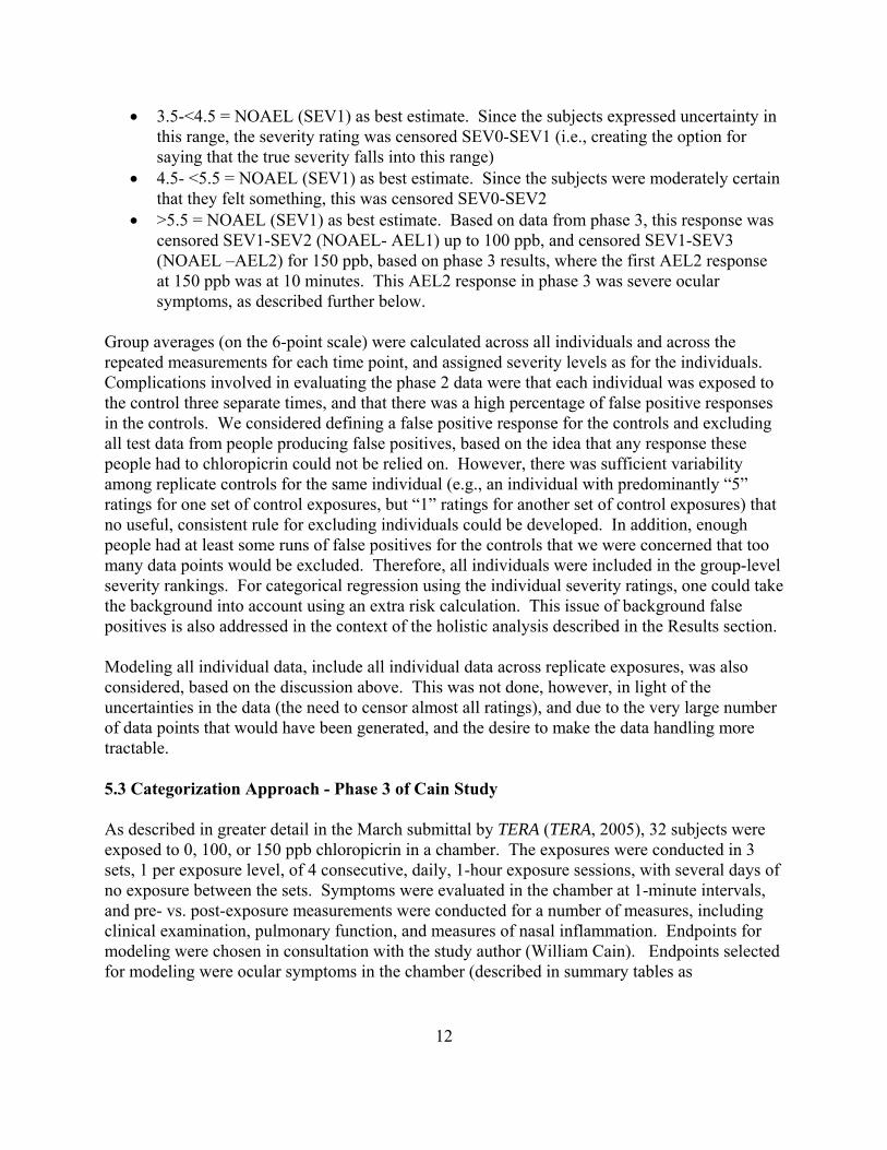
• 3.5-<4.5 = NOAEL (SEV1) as best estimate. Since the subjects expressed uncertainty in this range, the severity rating was censored SEV0-SEV1 (i.e., creating the option for saying that the true severity falls into this range)

• 4.5- <5.5 = NOAEL (SEV1) as best estimate. Since the subjects were moderately certain that they felt something, this was censored SEV0-SEV2

• >5.5 = NOAEL (SEV1) as best estimate. Based on data from phase 3, this response was censored SEV1-SEV2 (NOAEL- AEL1) up to 100 ppb, and censored SEV1-SEV3 (NOAEL –AEL2) for 150 ppb, based on phase 3 results, where the first AEL2 response at 150 ppb was at 10 minutes. This AEL2 response in phase 3 was severe ocular symptoms, as described further below.

Group averages (on the 6-point scale) were calculated across all individuals and across the repeated measurements for each time point, and assigned severity levels as for the individuals. Complications involved in evaluating the phase 2 data were that each individual was exposed to the control three separate times, and that there was a high percentage of false positive responses in the controls. We considered defining a false positive response for the controls and excluding all test data from people producing false positives, based on the idea that any response these people had to chloropicrin could not be relied on. However, there was sufficient variability among replicate controls for the same individual (e.g., an individual with predominantly “5” ratings for one set of control exposures, but “1” ratings for another set of control exposures) that no useful, consistent rule for excluding individuals could be developed. In addition, enough people had at least some runs of false positives for the controls that we were concerned that too many data points would be excluded. Therefore, all individuals were included in the group-level severity rankings. For categorical regression using the individual severity ratings, one could take the background into account using an extra risk calculation. This issue of background false positives is also addressed in the context of the holistic analysis described in the Results section. Modeling all individual data, include all individual data across replicate exposures, was also considered, based on the discussion above. This was not done, however, in light of the uncertainties in the data (the need to censor almost all ratings), and due to the very large number of data points that would have been generated, and the desire to make the data handling more tractable. 5.3 Categorization Approach - Phase 3 of Cain Study As described in greater detail in the March submittal by TERA (TERA, 2005), 32 subjects were exposed to 0, 100, or 150 ppb chloropicrin in a chamber. The exposures were conducted in 3 sets, 1 per exposure level, of 4 consecutive, daily, 1-hour exposure sessions, with several days of no exposure between the sets. Symptoms were evaluated in the chamber at 1-minute intervals, and pre- vs. post-exposure measurements were conducted for a number of measures, including clinical examination, pulmonary function, and measures of nasal inflammation. Endpoints for modeling were chosen in consultation with the study author (William Cain). Endpoints selected for modeling were ocular symptoms in the chamber (described in summary tables as

13

chemesthesis), nasal NO (an endpoint suggestive of inflammation), and inspiratory flow4. These endpoints were chosen based on the endpoints showing the largest changes (ocular symptoms), and statistical significance, as reported in the study based on analysis of the average data. Individual data for other endpoints, such as FVC and FEV1, were also evaluated in choosing the data to model, to ensure that individuals with clinically significant changes for these endpoints were not missed. Using a criterion of 20% change (pre vs. post-exposure), based on common definitions of clinical significance for spirometry, no individuals had an effect on FEV1, and only one individual had a barely significant effect on FVC. The following bullets describe how severity levels were assigned for each endpoint. Ocular symptoms were rated at 30 seconds and at every minute of the 1-hour exposures by the subjects while in the chamber, using the following scale. The descriptive term is shown in parentheses, followed by the severity rating using the 5-point scale described above. No translation of numerical severity ratings was needed, since the numerical severity ratings used by Cain are the same as the designated numerical ratings for the corresponding category.

• 0 (No Symptoms; NOEL) • 1 (Mild, Symptom present, but minimal awareness, easily tolerated; NOAEL) • 2 (Symptom definite and bothersome, but tolerated; AEL1) • 3 (Severe; symptom hard to tolerate and can interfere with activities of daily living or

sleeping; AEL2)

The following approach was used to determine the severity rating for each individual at each measured time point (i.e., minutes) and concentration across the 4 replicate exposure days. (Using this approach, each person would have 61 averaged measurements at each of the three concentrations.) First, because there were no significant differences or trends across the 4 exposure days for each concentration (Cain, 2004), the results at each time point for each individual were averaged across the 4 exposure days. This resulted in an average response for each individual for each time point and concentration. As for the Phase 2 data, an additional reason for averaging the results for each individual across replicate exposure days was to ensure that the data manipulation required to develop input files was reasonably tractable5. In addition, the use of multiple time points for each individual captured some of the intra-individual variability, although visual inspection of the data (as well as human nature) suggests that there was more intra-individual variability between identical exposures than between time points (in the plateau region) within a given chamber exposure. Thus, as described above, averaging each individual’s response across replicate exposure days did not capture the full extent of the intra-individual variability. Nonetheless, individual severity ratings, based on the average across replicate exposure days, was used for all of the categorical regression modeling, except where otherwise noted.

4Inspiratory flow was initially chosen based on advice from Dr. Cain that this endpoint is more sensitive than expiratory flow. This was confirmed based on the study report, which described decreased inspiratory flow as statistically significant, and the decrease in expiratory flow as only being “nearly significant.” 5 Note that all averaging described in this paragraph was across data for the same individual; only the averaging mentioned in the next paragraph, for the group-level severity rating, was across individuals.

14

To determine the incidence of individual severity ratings for each time point, the number of individuals with average severity ratings <0.5 (corresponding to SEV0, NOEL), ≥0.5 and <1.5 (corresponding to SEV1, NOAEL), and so on, were determined at each time point.6 Thus, for example, a given time/concentration data point might have 12 individuals with SEV0, 10 with SEV1, 8 with SEV2, and 2 rated as SEV3. This range in severity ratings across individuals for a given data point illustrates the range in sensitivity among the test subjects. No human subjects were classified as SEV4. The cutpoint of ≥1.5 was chosen based on the idea that a severity rating of 1 is NOAEL, 2 is AEL1, and the transition between NOAEL and AEL1 could be considered to occur halfway in between. This approach is analogous to the designation by Cain (2004) that a response of “yes” in Phase 3 is any response above 3.5. The choice of a cutpoint of ≥1.5 was also consistent with the results of the holistic analysis, described in Section 7.1. Other cutpoints for the Phase 3 ocular symptoms are possible. For example, one could argue that any value above 1 is in the AEL1 zone. This would increase the apparent response, and decrease the BMCs and EC10 values calculated in the modeling (a cutpoint of 1). Conversely, one could judge that the response is not adverse until a response of 2 is achieved (corresponding to a cutpoint of 2.0, and removing the issue of rounding). In that case, the apparent response would be lower, and the resulting BMCs and EC10 values would be higher. Cutpoints of 1 and 2 were not judged to be appropriate, however, for the use of averaged responses. For example, a cutpoint of 2 would imply that either all responses were “2” (an unlikely occurrence), or that all responses of “1” were counterbalanced by a response of “3,” and this was not considered a health-protective approach. Conversely, a cutpoint of greater than 1 would imply that most responses were “1” (minimal awareness), and all responses of “2” were counterbalanced by a response of “0”; this was not considered consistent with the definition of an adverse effect. To develop a group severity rating for each time point, the individual severity ratings described in the previous paragraph were averaged across individuals for each time point and rounded. This resulted in 61 severity ratings for each concentration, representing the average across individuals and across replicate days. Using this approach, the group-level severity for 100 ppm was SEV0 through 31 minutes, and SEV1 at most time points thereafter; at 150 ppm, the severity was SEV0 through 8 minutes, and then SEV1 at all time points thereafter. These averages are consistent with the results shown in Figure 20 of the Cain study. This group-level rating was used to provide initial information regarding the trends observed on average, but the modeling focused on the individual data. Both nasal NO (NO Rhino) and inspiratory flow (INS) were measured before and after each 1-hour exposure. Based on consultation with Dr. Cain and his colleague Dr. Jalowayski, a 25% increase (post vs. pre) in NO Rhino, or a 25% decrease in inspiratory flow, was considered clinically significant (AEL1). Use of this definition in the BMC modeling is described below. Late in the project, Dr. Jalowayski provided supplemental information that Dr. Vogt, who

6 It was noted that this approach biases ratings to the higher numbers, since ratings <0 are not possible, and the average of the four days will either end in 0 or 0.5. To address this issue, a sensitivity analysis could be conducted in which average values ending in 5 are rounded down. This issue of the unequal rounding applied only to the categorical regression input data, where only a small number of data points were averaged for each time point, and not to the BMC modeling, as described further below.

15

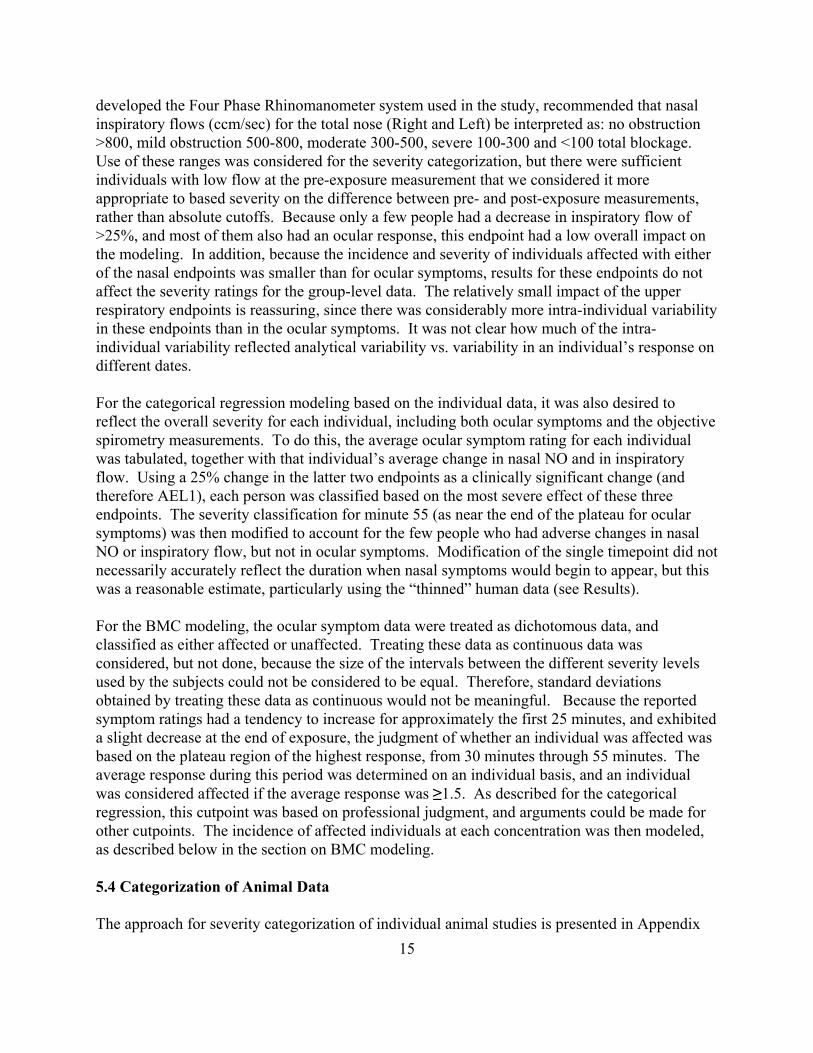
developed the Four Phase Rhinomanometer system used in the study, recommended that nasal inspiratory flows (ccm/sec) for the total nose (Right and Left) be interpreted as: no obstruction >800, mild obstruction 500-800, moderate 300-500, severe 100-300 and <100 total blockage. Use of these ranges was considered for the severity categorization, but there were sufficient individuals with low flow at the pre-exposure measurement that we considered it more appropriate to based severity on the difference between pre- and post-exposure measurements, rather than absolute cutoffs. Because only a few people had a decrease in inspiratory flow of >25%, and most of them also had an ocular response, this endpoint had a low overall impact on the modeling. In addition, because the incidence and severity of individuals affected with either of the nasal endpoints was smaller than for ocular symptoms, results for these endpoints do not affect the severity ratings for the group-level data. The relatively small impact of the upper respiratory endpoints is reassuring, since there was considerably more intra-individual variability in these endpoints than in the ocular symptoms. It was not clear how much of the intra-individual variability reflected analytical variability vs. variability in an individual’s response on different dates. For the categorical regression modeling based on the individual data, it was also desired to reflect the overall severity for each individual, including both ocular symptoms and the objective spirometry measurements. To do this, the average ocular symptom rating for each individual was tabulated, together with that individual’s average change in nasal NO and in inspiratory flow. Using a 25% change in the latter two endpoints as a clinically significant change (and therefore AEL1), each person was classified based on the most severe effect of these three endpoints. The severity classification for minute 55 (as near the end of the plateau for ocular symptoms) was then modified to account for the few people who had adverse changes in nasal NO or inspiratory flow, but not in ocular symptoms. Modification of the single timepoint did not necessarily accurately reflect the duration when nasal symptoms would begin to appear, but this was a reasonable estimate, particularly using the “thinned” human data (see Results). For the BMC modeling, the ocular symptom data were treated as dichotomous data, and classified as either affected or unaffected. Treating these data as continuous data was considered, but not done, because the size of the intervals between the different severity levels used by the subjects could not be considered to be equal. Therefore, standard deviations obtained by treating these data as continuous would not be meaningful. Because the reported symptom ratings had a tendency to increase for approximately the first 25 minutes, and exhibited a slight decrease at the end of exposure, the judgment of whether an individual was affected was based on the plateau region of the highest response, from 30 minutes through 55 minutes. The average response during this period was determined on an individual basis, and an individual was considered affected if the average response was ≥1.5. As described for the categorical regression, this cutpoint was based on professional judgment, and arguments could be made for other cutpoints. The incidence of affected individuals at each concentration was then modeled, as described below in the section on BMC modeling. 5.4 Categorization of Animal Data The approach for severity categorization of individual animal studies is presented in Appendix

16

D. All available animal studies were initially considered for categorization, based on studies identified by CMTF, and as verified for completeness by review of the recent USEPA OPP assessment. No independent literature searching was conducted. The duration of exposure used in the modeling was the total time of exposure, excluding time between exposures. Thus, for a 13-week study in which the animals were exposed 6 hours/day, 5 days/week, the total duration was 6 x 5 x 13 = 390 hours. This approach assumed that length of time between exposures did not affect the severity of response. This assumption may not have been completely accurate, since it could not take into account any repair that occurred between exposures. However, since the longer-term studies all used a 6 hour/day, 5 day/week approach, the approach was consistent across the longer-term studies, although there may have been some inconsistencies with the shorter-term data. The developmental toxicity studies were considered separately. The developmental study in rats (Schardein, 1993) conducted gross necropsy in the dams, but no histopathology evaluation, and so may have missed respiratory effects. The developmental study in rabbits (York, 1993) did include histopathology evaluation of the dams, including the respiratory tract. However, because the dams were sacrificed 9 days after the last exposure, the severity of the effect could have been underestimated, since the post-exposure period would have allowed for some recovery. Severity categorization for the two generation reproduction study in rats (Schardein, 1994) was not conducted for a number of reasons, including the absence of lung weight data, high background in controls, and exposure for 7 days/week. All modeling was conducted based on the exposure concentration, without additional adjustments for human equivalent concentrations (HECs), which take into account interspecies differences in tissue dose. For respiratory effects of acute exposures to vapors, EPA guidance (U.S. EPA, 1998) is that the HEC is the same as the exposure concentration. For longer-term exposures, the HEC depends on the target (e.g., nasal vs. tracheobronchial), as well as the body weight of the animal. To avoid apparent inconsistencies in the concentration-duration-response from different HECs for the same concentration at different durations, the initial analysis did not include the HECs. Including the HECs would also mean developing separate sets of input data based on nasal and tracheobronchial effects, since each of these regions has different HEC exposure concentrations, and different incidences of affected animals. As an initial indication of the impact of using exposure concentration rather than HECs, the group-level data were plotted using the HECs, with only some initial attempts made at modeling the data (Appendix A). A key aspect of categorical regression is that a given severity level should mean the same thing, regardless of the endpoint. Fulfilling this requirement was a particular challenge in combining the animal and human data. For example, symptoms judged as “hard to tolerate” were considered to be AEL2 (moderate severity), even though no evidence of inflammation was observed based on clinical examination. In contrast, at least moderate histopathology was required before an animal endpoint was considered to be of moderate severity. To some degree, this discrepancy reflects the desire to recognize tolerability of irritation in humans, while being consistent with standard interpretation of histopathology findings. However, this approach introduced some uncertainties and inconsistencies in the analysis; implications of these judgments will be evaluated as part of the categorical regression analysis.

17

6.0 BMC MODELING APPROACH BMC modeling was conducted only for Phase 3 of the Cain (2004) study described above. The experimental design is a repeated measures design because subjects were exposed repeatedly throughout the experiment. Each subject was exposed to three concentrations of chloropicrin (0, 100, and 150 ppb), and exposure to each concentration was repeated over 4 consecutive days. While this experimental design has advantages, the random effects introduced by the repeated measures present added complications to the analysis of the data and derivation of a benchmark concentration. The multiple measures from each individual can introduce additional variability in the response that may require modeling to accurately estimate the BMCL. To evaluate the effect of the repeated measures, benchmark concentrations for the continuous (upper respiratory) endpoints were derived by analyzing the repeated measures in up to three different ways: 1) treating each measurement as an independent observation (i.e., no repeated measures); 2) averaging the pre- vs. post- changes across sessions for each individual at each concentration to obtain one measure of the change for each person at each concentration; and 3) using nonlinear mixed effects modeling to account for the repeated measures. The only difference among the modeling approaches was the method for addressing intra-individual variability. Regardless of the modeling approach, the modeling was done in a way to capture the inter-individual variability in response at each exposure concentration and in the controls. The former two modeling approaches were implemented using U.S. EPA’s BMDS program, while the latter was implemented using S-Plus®. An analogous set of approaches was used for the ocular symptoms, a quantal endpoint. In that case, the accounting for the repeated measures was done using the clustering function of ToxTools and using the nested models of BMDS. The resulting benchmark concentrations derived using these approaches were compared to evaluate the magnitude of the effect of the repeated measures. 6.1 Continuous Data Modeling Nasal NO (NO rhino, a measure of inflammation) and inspiratory flow to the nose (INS) were modeled using continuous concentration-response models. Based on consultation with Drs. Cain and Jalowayski, the BMR was defined as a 25% change (increase in NO or decrease in INS) compared to an individual’s pre-exposure measurement, as a clinically significant change on an individual basis. The BMDS software allows one to specify a cutoff point for the BMR, but it is a cutoff for the mean response and (for a normally-distributed population) corresponds to 50% of the population above and 50% below the BMR. The cutoff for the mean that corresponds to a 10% extra risk of an individual exceeding 25% was found using the following procedure:

• Use BMDS to estimate the background mean [mu(0)] and standard deviation (s) of the responses. The mean and standard deviation estimated by BMDS was used, rather than the actual mean and standard deviation of the data, so that the background probability used in calculating the cutoff is the same as the starting point that BMDS uses for the benchmark dose modeling.

18

• Compute the background probability, P(0), of exceeding the cutoff assuming the responses are normally distributed with mean mu(0) and standard deviation s.

• Compute probability yielding 10% extra risk, P(d), from [P(d)-P(0)]/[1-P(0)] = 0.1 • The cutoff for BMDS is the mean M that will give a P(d) probability of exceeding the

cutoff7 This method is generally analogous to that described by Gaylor and Slikker (1990) and Crump (1995) for expressing BMRs for continuous data in terms of percent risk. The procedure above assumes that the data are normally distributed with a mean that is a function of dose, and constant variance. Based on the equal variance test in BMDS, which indicates that a homogeneous variance appears to be appropriate for these data, this assumption appears appropriate. While the homogeneous variance appears to be appropriate for modeling the BMC, a further uncertainty is whether the variance of responses can be assumed to be the same when computing the BMCL; this is the major uncertainty with this approach to calculating the mean cutoff value. In doing the modeling, the variance parameter (as well as the other parameters in the model) is adjusted to obtain the upper bound on the dose-response curve that is used to compute the BMCL. However, for these data, it is unlikely that the assumption of equal variances introduces much error, because the standard errors for the variance estimates are relatively small (an order of magnitude less than the maximum likelihood estimate for the variance parameter). This assumption could be removed by using the parameter values obtained for the upper bound response curve calculation to compute a new cutoff and BMCL. Unfortunately, these values are not supplied by the BMDS program, although they may be obtained by using different software. A transformation was performed on the data to decrease the impact of some extremely high values, and to make the data appear more normally distributed. The natural logarithm of the ratio of the post-exposure to the pre-exposure value was used instead of the percent change. 6.2 Quantal Data Modeling The ocular symptom severity scores were modeled as dichotomous data. Based on inspection of the responses revealing a plateau after about 25 minutes of exposure and a possible drop in severity over the last 5 minutes of the 1-hour exposure, the average score from 30 minutes to 55 minutes for each subject was used. The incidence in each concentration group was computed as the number of scores above 1.5. (Other alternatives are presented in Appendix A.) In addition,

7 For example, for the averaged nasal NO data, BMDS was run and the estimated background mean and standard deviation (expressed as fractions) were 0.016 and 0.12, respectively. The background probability or incidence is calculated using P0 = 1 – N(ln(1.25), 0.016, 0.12) = 0.037, where N is the cumulative normal distribution, and ln(1.25) is the critical 25% cutoff after log-transforming the data. Next, the probability exceeding the cutoff that corresponds to a 10% extra risk is P(d) = 0.1*(1-P0)+P0 = 0.13. (In other words, this expression converts 10% extra risk to a simple probability, given the background response.) Finally, the target mean (delta) is computed by solving the expression N-1(0.87, delta, 0.12) = ln(1.25), where N-1() is the inverse of the standard normal distribution (a percentile, mean, and standard deviation are supplied and the value corresponding to that percentile is returned), and 0.87 = 1 – P(d). Delta is adjusted until the inverse normal function returns a value equal to the cutoff of ln(1.25).

19

the issue noted above regarding a bias in rounding was not relevant, since the approach of averaging across the 30-55 minute time period meant that average results other than 0, 0.5, 1, 1.5, 2, 2.5 were available. The resulting input data are presented in Table 1. Table 1. Ocular Symptom Incidence Calculated for Use in BMC Modeling

Concentration Incidence Using Cutpoint of ≥ 1.5

Percent Response

0 ppb 0/32 0% 100 ppb 2/32 6% 150 ppb 9/32 28% The benchmark response (BMR) was defined as 10% extra risk. 7.0 RESULTS 7.1 Benchmark Concentrations As discussed above, several different approaches were used for the BMC modeling, to address the issue of multiple measures. The full description of the approach used is shown in Appendix A, along with plots of the BMC models of choice. The following text presents the preferred approach to modeling nasal NO and ocular symptoms endpoints. Inspiratory flow (also an upper respiratory endpoint) was also modeled, but good fit to the data was not possible (i.e., goodness-of-fit p value was <0.1 or only slightly greater than 0.1, and the visual fit was poor), because the response was non-monotonic (first decreasing, then increasing, with increasing dose). Therefore, the results for inspiratory flow are presented only in Appendix A. In all of the modeling for the nasal NO (a continuous endpoint), the mean and standard deviation was used, to take into account the individual variability in response. In one set of modeling, the average response for each individual across the replicate exposures (hereafter referred to as the “averaged” approach) was included in the calculation of the standard deviation, while in the second set, each replicate exposure was considered an independent evaluation. As described in Appendix A, neither of these approaches appropriately account for the intraindividual variability. As further described in Appendix A, mixed effects modeling (MEM) appropriately accounts for the interindividual variability. Using that approach, the BMC is similar to that using the “averaged” approach, while the BMCL is similar to (but slightly lower than) that based on considering each measurement to be independent. However, results of MEM approach are not used as the basis for the BMCL for the nasal NO endpoint, due to uncertainties regarding implementation of the methods for calculating the BMCL in S-Plus. Therefore, as a best estimate, the results from the “averaged” and independent approaches can be averaged. Table 2 presents the results of the BMC modeling (using the mean and standard deviation of the population, as described above), using the approach of averaging each individual across replicate exposures, and using the approach of treating each exposure independently. The BMR was defined as 10% of the population having at least a 25% increase in nasal NO (post- vs. pre-

20

exposure, considered to be a clinically significant change on an individual basis). Using the average of the two approaches, the BMC is 130 ppb and the BMCL is 90 ppb. The exact choice of the BMCL for this endpoint is, however, of less concern, since the ocular symptoms are judged to be the critical effect. Table 2. Benchmark Concentrations for Nasal NO

BMR Endpoint Approach Delta1 p-value2 BMC (ppb)

BMCL (ppb)

10% of the population

having a 25% change in

effect

Nasal NO Averaged3 0.094 0.54 140 100

Independent4 0.083 0.5 120 80

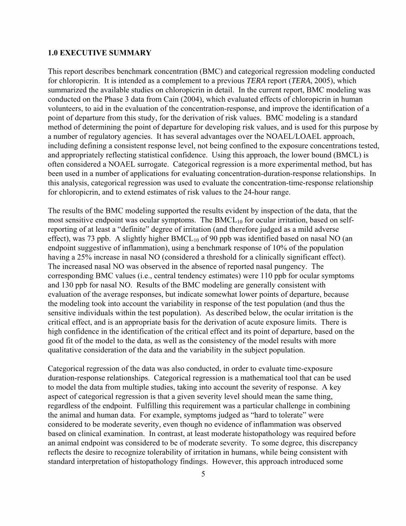
1 Delta is the BMR – the mean response (expressed as % change in post- vs. pre-exposure nasal NO) that corresponds to 10% of the subjects being affected. In other words, the mean value for post-exposure vs. pre-exposure nasal NO (the natural log-transformed ratio of post- to pre-exposure NO) in the control group was approximately 1.2%. A delta of 0.094 means that if 9.4 percentage points (on a log-transformed scale) were added to the mean response (resulting in a mean of approximately 11% change [natural log-transformed, corresponding to a ratio of 1.12] in NO post-exposure vs. pre-exposure), the distribution would be shifted sufficiently that 10% of the subjects would exceed the 25% cutoff for change in NO 2 The p value is a measure of the goodness-of-fit, with higher p values reflecting better fit. A goodness-of-fit p value of 1.0 reflects perfect fit to the data. A minimum p value of 0.1 is generally considered necessary for a model to be considered, although visual fit and local fit also need to be evaluated. 3 Averaged over four sessions for each subject at each concentration. Thus, the mean was based on an N of 32. 4 All measurements treated as independent samples. Thus, the mean was based on an N of up to 128. Table 3 shows the BMCs and the BMCLs calculated for the ocular symptoms for the best-fitting models, and Figure 1 presents the modeling results for one example of a well-fitting model. The x axis is concentration (in ppb), and the y axis is the fraction of people who had an adverse response (defined as an average response of at least 1.5 during the plateau period). As for the continuous endpoint, alternative modeling approaches were used to address the repeated measures resulting from exposing each individual on four separate days; these alternatives are described in Appendix A. As described in Appendix A, the approach ultimately used for the quantal endpoint was to take the average severity score for each individual across the replicate days, in order to determine the response incidence. BMDS contains a number of different mathematical functions (models) that can be used to fit the data, and current guidance is to run all of them. The full analysis is summarized in Appendix A. Perfect fit to the data was obtained using the gamma, log-logistic log-probit, and Weibull models. The same BMC of 110 ppb was estimated with all of these models, but there was some small variability in the BMCL. Therefore, the BMCL for the ocular endpoint using the cutpoint of 1.5 was calculated by averaging the BMCLs across the four models with perfect fit. The resulting BMCL is 73 ppb.

Figure 1. Gamma Model fit to the Ocular Symptoms Data (vs. concentration in ppb), using Response Incidence Based on Average Across Replicate Exposures and a Cutpoint of ≥1.5

0

0.1

0.2

0.3

0.4

0.5

0 20 40 60 80 100 120 140 160

Frac

tion

Affe

cted

dose

Gamma Multi-Hit Model with 0.95 Confidence Level

15:50 06/08 2005

BMDL BMD

Gamma Multi-Hit

Table 3. Benchmark Concentrations Calculated for Ocular Symptoms

Model AIC1 P-Value2 BMC BMCL

Gamma 57 1 110 71 Log-logistic 57 1 110 72 Log-probit 57 1 110 76 Weibull 57 1 110 71

1 AIC is Akaike’s information criterion, a measure of fit that adjusts for the number of parameters, where the smaller the AIC, the better the fit. The AIC is used to compare across models for a given data set, but should not be used to compare across datasets. Because the AIC depends on the actual data set, no typical or maximum value can be specified. 2 The p value is a measure of the goodness-of-fit, with higher p values reflecting better fit. The maximum possible value is 1.0 Table 4 summarizes the BMCLs for the two endpoints that were successfully modeled. No BMCL could be calculated for the inspiratory flow endpoint. Ocular symptoms are judged to be

21

22

the critical effect, with a BMCL of 73 ppb for a 1-hour exposure. This endpoint is supported by the increased nasal NO, with an averaged best estimate of the BMCL of 90 ppb. Table 4. Summary of Benchmark Modeling Results for Cain (2004)

Endpoint BMC (ppb) BMCL (ppb) Ocular Symptoms 110 73 Nasal NO 130 90 As a test of whether the results of the modeling were consistent with biological judgment regarding the severity of the response for each individual, a holistic judgment was made regarding whether each individual in Phase 2 and Phase 3 of the Cain (2004) study was responding. This judgment was based on an overall evaluation of the data for each individual, taking into account the trends, with particular attention to the response at the initial time points. Note that, for Phase 2, a response was defined as whether the individual felt something with the eye. For Phase 3, a severity rating was assigned holistically for each individual (allowing intermediate severity ratings of 0.5, 1.5, 2.5) across the four replicate trials, and then the holistic severity rating for the control exposure for that individual was subtracted off. The individual was considered a responder if the net response was at least a severity rating of 1.5. Thus, for Phase 3, a response was defined as a minimum rating for severity of irritation. This holistic evaluation was conducted independently by two senior toxicologists; results are shown in Table 5. The range of results reflects the degree of judgment in the ratings, but generally consistent results were obtained from the two sets of analyses. Comparing the results with Table 4 indicates that the BMC results are biologically reasonable. The BMC (maximum likelihood estimate) for a 10% response was 110 ppb, and the estimated Phase 3 response at 100 ppb was close to 10%. Similarly, the percentage of subjects detecting the chloropicrin at 75 ppb in Phase 2 (even after accounting for the high false positives in the controls) suggests that the BMCL for ocular effects of 73 ppb falls into the range at which the test subjects started to “feel” the chemical in their eyes, and thus may not be unreasonable as a point of departure from which to derive a “safe” concentration. Note also that the holistic evaluation of response in Phase 3 results in % responses that are comparable to, but slightly higher than, the percentages used as input to the modeling (see Table 1).

23

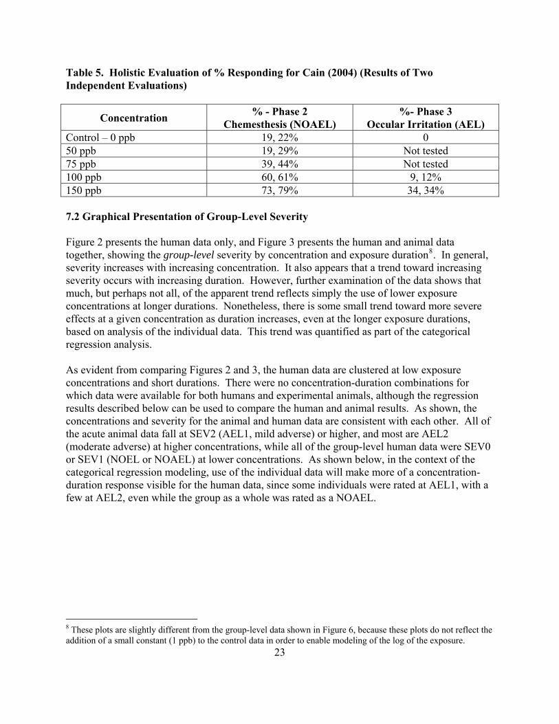
Table 5. Holistic Evaluation of % Responding for Cain (2004) (Results of Two Independent Evaluations)

Concentration % - Phase 2 Chemesthesis (NOAEL)

%- Phase 3 Occular Irritation (AEL)

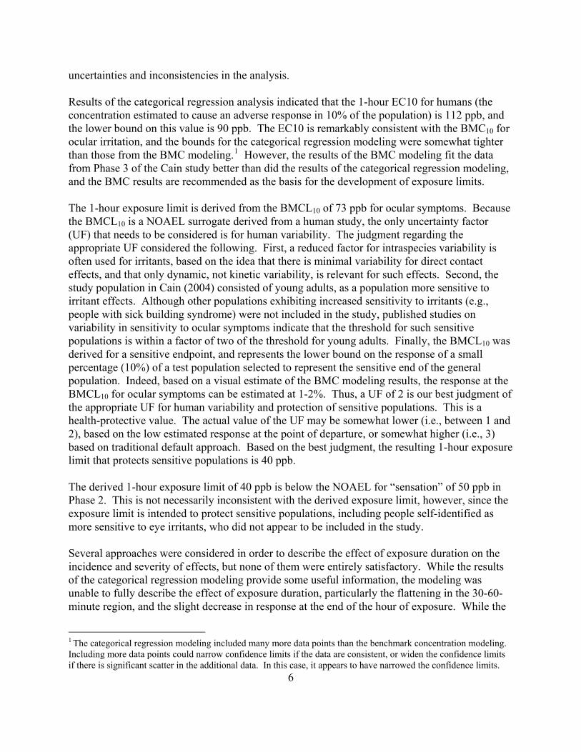
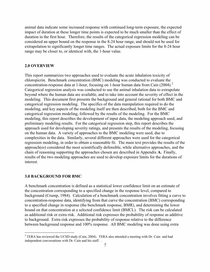
Control – 0 ppb 19, 22% 0 50 ppb 19, 29% Not tested 75 ppb 39, 44% Not tested 100 ppb 60, 61% 9, 12% 150 ppb 73, 79% 34, 34% 7.2 Graphical Presentation of Group-Level Severity Figure 2 presents the human data only, and Figure 3 presents the human and animal data together, showing the group-level severity by concentration and exposure duration8. In general, severity increases with increasing concentration. It also appears that a trend toward increasing severity occurs with increasing duration. However, further examination of the data shows that much, but perhaps not all, of the apparent trend reflects simply the use of lower exposure concentrations at longer durations. Nonetheless, there is some small trend toward more severe effects at a given concentration as duration increases, even at the longer exposure durations, based on analysis of the individual data. This trend was quantified as part of the categorical regression analysis. As evident from comparing Figures 2 and 3, the human data are clustered at low exposure concentrations and short durations. There were no concentration-duration combinations for which data were available for both humans and experimental animals, although the regression results described below can be used to compare the human and animal results. As shown, the concentrations and severity for the animal and human data are consistent with each other. All of the acute animal data fall at SEV2 (AEL1, mild adverse) or higher, and most are AEL2 (moderate adverse) at higher concentrations, while all of the group-level human data were SEV0 or SEV1 (NOEL or NOAEL) at lower concentrations. As shown below, in the context of the categorical regression modeling, use of the individual data will make more of a concentration-duration response visible for the human data, since some individuals were rated at AEL1, with a few at AEL2, even while the group as a whole was rated as a NOAEL.

8 These plots are slightly different from the group-level data shown in Figure 6, because these plots do not reflect the addition of a small constant (1 ppb) to the control data in order to enable modeling of the log of the exposure.

Figure 2. Human Group-Level Severity Scores - Phases 2 and 3

Human Severity Scores

0

0.02

0.04

0.06

0.08

0.1

0.12

0.14

0.16

0 0.2 0.4 0.6 0.8 1 1.2

Hours

ppm Sev0

Sev1

24

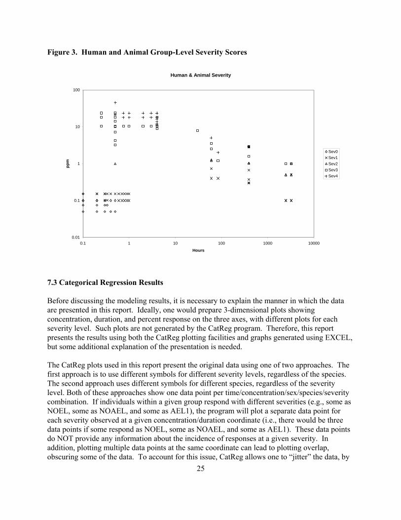
Figure 3. Human and Animal Group-Level Severity Scores

Human & Animal Severity

0.01

0.1

1

10

100

0.1 1 10 100 1000 10000

Hours

ppm

Sev0Sev1Sev2Sev3Sev4

7.3 Categorical Regression Results Before discussing the modeling results, it is necessary to explain the manner in which the data are presented in this report. Ideally, one would prepare 3-dimensional plots showing concentration, duration, and percent response on the three axes, with different plots for each severity level. Such plots are not generated by the CatReg program. Therefore, this report presents the results using both the CatReg plotting facilities and graphs generated using EXCEL, but some additional explanation of the presentation is needed. The CatReg plots used in this report present the original data using one of two approaches. The first approach is to use different symbols for different severity levels, regardless of the species. The second approach uses different symbols for different species, regardless of the severity level. Both of these approaches show one data point per time/concentration/sex/species/severity combination. If individuals within a given group respond with different severities (e.g., some as NOEL, some as NOAEL, and some as AEL1), the program will plot a separate data point for each severity observed at a given concentration/duration coordinate (i.e., there would be three data points if some respond as NOEL, some as NOAEL, and some as AEL1). These data points do NOT provide any information about the incidence of responses at a given severity. In addition, plotting multiple data points at the same coordinate can lead to plotting overlap, obscuring some of the data. To account for this issue, CatReg allows one to “jitter” the data, by 25

26

slightly changing the position of data points to minimize overlap. While this approach works well in general, the jittering for the control group resulted in large displacements of the data points. Therefore, the data points at <50 ppb (aside from the 1 ppb data) are erroneously plotted, and reflect control data. This erroneous plotting did NOT affect the modeling results. In addition, the modeling was conducted using the log of concentration and of time. In order to make it possible to plot the control data, a small constant of 1 ppb was added to all of the concentration data. This small increment would not have a substantive impact on the modeling results, but it means that the control data are plotted as 1 ppb in the analyses. For both types of plotting with CatReg, the curves show the concentration-time combinations resulting in an estimated 10% response (referred to as EC10 curves). Some plots show the best estimates of the curves by species (“strata EC10 lines”) while others show a single best estimate curve, with 95% confidence limits on the curve (“EC10 line with 95% confidence bounds”). Unless otherwise specified, the best estimate of severity for each group was used (“BestNum”). A sensitivity analysis for the model of choice was also conducted analysis using the “censored” data, where a range of severities was assigned when there were uncertainties based on the available data. Because CatReg shows a data point for each severity represented, regardless of the percent of individuals affected, EXCEL spreadsheets were used to communicate the degree of response at a given coordinate. This was done in two ways. First, concentration-time plots were prepared showing the group-level severity, together with the EC10 curves calculated using CatReg. This approach has the advantage of showing EC10 curves in relationship to the average severity level of a group, but has the disadvantage that it does not capture the variability in response, and thus the response of sensitive individuals. The second approach was to show probability plots at specific time cross-sections of the curve, in order to capture the variability in the human response, and to compare the calculated curves with the available data, when possible. These plots show the actual AEL1 incidence for humans (from Cain, 2004), plotted versus the curves calculated by CatReg. Similar curves for the predicted human response are presented for 8 hours and 24 hours, to provide better illustration of the predicted concentration-response, but no human data are available for these time points. Several alternative approaches to modeling the data were explored in the effort to obtain results that both agreed with the data and were biologically plausible. These early efforts are described in Appendix A, and only the final preferred model is discussed in the main body of this report. The data for the final model used four severity categories to describe the data, rather than the five categories that were described in the methods section. As described in the appendix, the original categorization was changed to combine the NOEL (SEV0) and NOAEL (SEV1) into severity level 0, and the remaining severity categories were shifted downward. While this approach was necessary in order to obtain reasonable results, a disadvantage of removing the NOEL category is that some of the concentration-duration-response information in the Cain study was lost. Another modification to the full data set was that the human data were “thinned” to include only data from 0.5 minutes (the first time point), 20 minutes (as the terminus of some Phase 2 data), 30 minutes, 45 minutes, and 60 minutes. In addition, the 55-minute time point was included, since this time point was the approximate end of the plateau in response in the

27

Phase 3 study, before the decreased response in the last few minutes. This “thinning” was done in order to avoid over-weighting the human response. As described above, the 55-minute time point was also modified to include the maximal response of any individual, taking into account the ocular symptoms, nasal NO, and inspiratory flow endpoints. We also evaluated the impact of excluding the developmental studies. As described above, the design of these studies differed from the other longer-term studies, so that the observed severities were not directly comparable. Removal of the developmental studies did not have a visible effect on the modeling results, but all further modeling was done without the developmental studies, to maximize the comparability of different studies. Appendix C presents the input data and explanation of the notation used. An electronic copy of the full input data for all of the animal and human data is available on request. The final model is the restricted cumulative odds model, logit link function, with log-transformed concentration parameter stratified by species, intercepts and log-transformed time parameter unstratified, and using the best estimate of severity (BestNum) rather than censored data. This model requires that the curves for the different severity levels be parallel. Attempts to test this assumption were not successful when using all of the human and animal data, because the model failed, and no further attempt was made to test this assumption. However, because all of the severity levels reflect the same general irritant mechanism, it is reasonable to expect that the severity curves will be parallel. Preliminary analyses also revealed that stratification of the concentration parameter (slope) by species, but maintaining a constant intercept term across species, resulted in reasonable shapes to the curve. The choice of link function had only a small impact on fit, but the logit link function resulted in the best fit (Table 6). Table 6. Summary Statistics for the Categorical Regressions Using the Data Set of Choice, Cumulative Odds Model

Distribution Link Censored? Deviance R2

Logistic logit N 2007 0.54 Normal probit N 2136 0.51 Gumbel Log-log N Failed ⎯ Logistic logit Y 1805 0.54

The lower the deviance for a given data set, the better the fit. The higher the R2 for a given data set, the better the fit. The maximum possible R2 is 1.0. The following text presents the graphical results of the categorical regression modeling, followed by a tabular presentation of some key numerical results. The implications of the results are then discussed briefly. These implications are addressed in more detail in the next section, in the context of derivation of exposure limits. Figure 4 shows the result of fitting the preferred model to the 4-category data. The lines on the plot show the SEV1 EC10, the concentration that results in a 10% probability of severity 1 or greater (i.e., AEL1 [mild adverse effect level] or worse), for humans, mice, and rats. Note that

28

the different symbols in the figure represent the concentration and time combinations for which data exist for different species; no information is presented on the severity level or response incidence observed at these various combinations of exposure concentration and time. Figure 5 shows the human data that were modeled and the calculated human EC10 line for AEL1, with 95% confidence bounds. The symbols in this figure represent the different response severities, though many of the points overlap and the figure does not show the number responding at each severity level. Figure 6 again shows the line for human AEL1 EC10 with 95% confidence bounds, with the model fit based on the individual data. In this plot, the individual data points reflect the group-level severity data to illustrate the general agreement of the model results with the overall, group-level response. It is important to note that the group-level severities shown in Figure 6 do not indicate that all individuals in the human study responded at severity 0, but that most of the group did; there are a few severity 1 and 2 scores in the higher concentration-time groups. (Similar principles apply to the plotting of the animal data.) The EC10 line for AEL1 falls at the upper end of the human group-level severity 0 data, reflecting the presence of individuals with AEL1 responses at these time points. Based on these figures, it appears that the AEL1 EC10 prediction is consistent with the human data and the biology, with only a moderately steep curve at short time points (evident on the log-log plot), and the expected flattening of the curve at longer durations. Figure 7 shows the 1-hour cross section of the probability of an AEL1 or greater response as a function of concentration. The curve in this figure is comparable to Figure 1 showing the BMC curve for the ocular symptom endpoint (because the overall response is driven primarily by the ocular symptoms, with a slight adjustment based on including the nasal endpoints). Based on this figure, it is clear that the fit to the human data is not as good as it was using the benchmark modeling. However, the categorical regression includes data over a wide range of time points in an attempt to understand concentration-time relationships and possibly extrapolate human response to longer time periods, while the BMC analysis focuses on the 1-hour human data only. Therefore, the results from the BMC modeling, rather than the CatReg modeling, should be used to estimate the response in humans after a 1-hour exposure to chloropicrin, though the CatReg results may be useful for extrapolating to longer exposures. Figure 8 shows the same cross sectional probability at 1, 8, and 24 hours. This figure illustrates the predicted gradual change in the EC10 (on the graph, the concentration where the plotted curves cross 0.1 probability) with time. There are no human data for comparison at 8 or 24 hours.

Figure 4. CatReg Plot of Human and Animal AEL1 EC10 (ppm)

Strata EC10 lines, Link = logit

Duration ( Hours )

Con

cent

ratio

n ( H

EC

)

0.01 0.10 1.00 10.00 100.00 1000.00

0.00

10.

010

0.10

01.

000

10.0

00

SEV1:HumanSEV1:MuSEV1:R

29

Figure 5. CatReg Plot of Human AEL1 (Mild Adverse) EC10 (ppm)

EC10 Line (SEV1:Human) with 95% Confidence Bounds, Link = logit

Duration ( Hours )

Con

cent

ratio

n ( H

EC

)

0.0 0.2 0.4 0.6 0.8 1.0

0.00

10.

005

0.05

00.

500

No effectSeverity 1Severity 2Severity 3Censored

30

Figure 6. EXCEL Plot of Human AEL1 EC10 (ppb) with 95% Confidence Bounds. Individual Data Modeled, but Data Points Represent Group-Level Severity for all Groups Modeled

Severity 1 (AEL1) EC10 and 95% Confidence Interval

1

10

100

1000

10000

100000

0.001 0.01 0.1 1 10 100 1000 10000

Hours

ppb

Human EC10Human: Sev0Mouse: Sev0Mouse: Sev1Mouse: Sev2Rat: Sev0Rat: Sev1Rat: Sev2Rat: Sev3

31

Figure 7. 1-Hour Cross Section of Incidence of AEL1 or Worse in Humans. Individual Points are Incidence Data from Phase 3, and Curve is Modeled Results from CatReg

1-Hour Probability of Severity 1 or Greater (AEL1 or Worse)

0

0.1

0.2

0.3

0 0.02 0.04 0.06 0.08 0.1 0.12 0.14 0.16 0.18 0.2

ppm

Prob

abili

ty

AEL1

32

Figure 8. 1-, 8-, and 24-Hour Cross Sections of Incidence of AEL1 or Worse in Humans

8-Hour

24-Hour

1-Hour

0

0.1

0.2

0.3

0 0.02 0.04 0.06 0.08 0.1 0.12 0.14 0.16 0.18 0.2

ppm

Prob

abili

ty

33

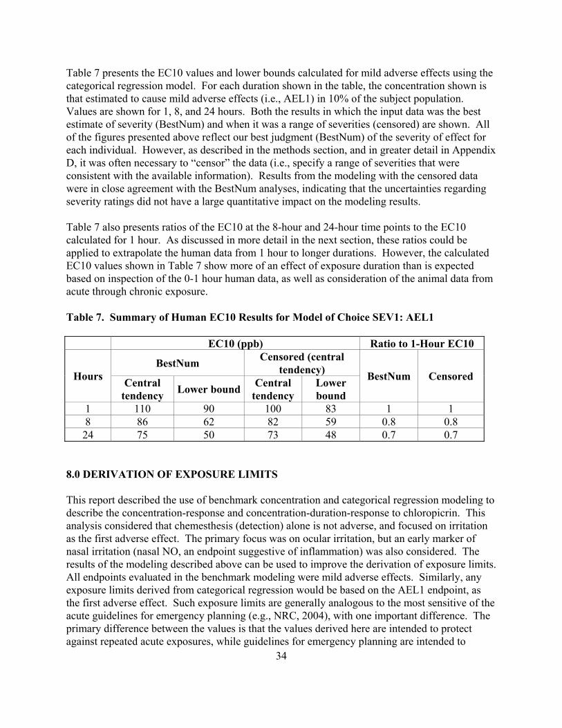
34

Table 7 presents the EC10 values and lower bounds calculated for mild adverse effects using the categorical regression model. For each duration shown in the table, the concentration shown is that estimated to cause mild adverse effects (i.e., AEL1) in 10% of the subject population. Values are shown for 1, 8, and 24 hours. Both the results in which the input data was the best estimate of severity (BestNum) and when it was a range of severities (censored) are shown. All of the figures presented above reflect our best judgment (BestNum) of the severity of effect for each individual. However, as described in the methods section, and in greater detail in Appendix D, it was often necessary to “censor” the data (i.e., specify a range of severities that were consistent with the available information). Results from the modeling with the censored data were in close agreement with the BestNum analyses, indicating that the uncertainties regarding severity ratings did not have a large quantitative impact on the modeling results. Table 7 also presents ratios of the EC10 at the 8-hour and 24-hour time points to the EC10 calculated for 1 hour. As discussed in more detail in the next section, these ratios could be applied to extrapolate the human data from 1 hour to longer durations. However, the calculated EC10 values shown in Table 7 show more of an effect of exposure duration than is expected based on inspection of the 0-1 hour human data, as well as consideration of the animal data from acute through chronic exposure. Table 7. Summary of Human EC10 Results for Model of Choice SEV1: AEL1

EC10 (ppb) Ratio to 1-Hour EC10

Hours BestNum Censored (central

tendency) BestNum Censored Central tendency Lower bound Central

tendency Lower bound

1 110 90 100 83 1 1 8 86 62 82 59 0.8 0.8 24 75 50 73 48 0.7 0.7

8.0 DERIVATION OF EXPOSURE LIMITS This report described the use of benchmark concentration and categorical regression modeling to describe the concentration-response and concentration-duration-response to chloropicrin. This analysis considered that chemesthesis (detection) alone is not adverse, and focused on irritation as the first adverse effect. The primary focus was on ocular irritation, but an early marker of nasal irritation (nasal NO, an endpoint suggestive of inflammation) was also considered. The results of the modeling described above can be used to improve the derivation of exposure limits. All endpoints evaluated in the benchmark modeling were mild adverse effects. Similarly, any exposure limits derived from categorical regression would be based on the AEL1 endpoint, as the first adverse effect. Such exposure limits are generally analogous to the most sensitive of the acute guidelines for emergency planning (e.g., NRC, 2004), with one important difference. The primary difference between the values is that the values derived here are intended to protect against repeated acute exposures, while guidelines for emergency planning are intended to

35

protect against a single event in a lifetime.9 Thus, the values derived here are more like an acute U.S. EPA RfC, California EPA REL, or the equivalent of an occupational short-term exposure limit (STEL) derived for the general public. Information on the concentration that would result in chemesthesis only (i.e., detection only), without irritation, could also be of interest. The data in Phase 2, which specifically address chemesthesis, show that 50 ppb for up to 30 minutes did not result in chemesthesis, whereas 75 ppb clearly shows this effect. Unfortunately, these data were not easily amenable to BMC modeling, although they may be amenable to more sophisticated concentration-response modeling approaches. Likewise, categorical regression did not yield meaningful results for chemesthesis from the 5-category approach, in which NOAELs and NOELs were separated. Moreover, the successful modeling described above, using the 4-category approach, did not distinguish no effect from chemesthesis, by our definition. Therefore, the rest of this analysis focuses on the threshold for AEL1 effects. The derivation of a 1-hour exposure limit is discussed first, since this is the longest duration within the range of the human data, and a common acute exposure limit. The available modeling results could easily be used to derive exposure limits for shorter durations, if desired, in light of the good fit of the categorical regression results in this region. Application of the modeling results to other common exposure durations of interest is also discussed. The first decision point in deriving the acute exposure limit is identification of the critical effect. As described in TERA (2005), the focus was on the data in the Cain (2004) study. This study was done in the species of interest, using a presumed sensitive population (healthy young adults, who have more refined odor and sensory ability than older adults), and identified a NOAEL. In contrast, the only available acute animal inhalation studies were conducted at high exposure levels that caused microscopic pathological findings (Hoffman, 1999a), or only measured the single endpoint of respiratory depression (Hoffman, 1999b). The acute animal data did not identify a NOAEL.

Biologically or statistically significant effects were seen for three endpoints in the Cain (2004) study, ocular symptoms, nasal NO, and inspiratory flow. While statistically significant decreases were observed for inspiratory flow, there was large variability and a nonmonotonic (decreasing, then increasing) concentration-response. No reliable BMCs could be calculated for this endpoint due to poor fit, and the overall assessment indicates that this endpoint is less sensitive than the other two, and therefore inspiratory flow was judged not to be the critical effect. BMCL modeling was done for nasal NO by defining the BMR as 10% of the subjects having a clinically significant (>25%) increase. Interestingly, the nasal endpoint was observed in the absence of self-reported nasal irritation. For ocular symptoms, the BMR was defined as 10% of the subjects having a response during the plateau region of at least 1.5 (i.e., symptoms defined at least half the time as definite and bothersome, but tolerated). The BMC modeling was able to fit the data well for both endpoints. While there were some concerns about appropriately accounting for the

9 Both the NRC values and values derived here are intended to protect the general population, including sensitive individuals, from adverse effects.

36

repeated measures resulting from the replicate exposures, the BMCLs calculated using the standard software (BMDS) were closely supported by those using more sophisticated techniques, for which there were some uncertainties that precluded their use in setting exposure limits (see Appendix A). Therefore, based on these definitions, the BMCL (lower 95% confidence limits on the BMC) for nasal NO was 90 ppb, and the BMCL for ocular symptoms was 73 ppb. The corresponding BMCs were 130 ppb and 110 ppb. Thus, consistent with the analysis in the earlier report (TERA, 2005), ocular symptoms are more sensitive than nasal effects, and represent our judgment of the critical effect. The BMC and it lower limit of 110 ppb and 73 ppb, respectively, are also consistent with the holistic evaluation of the data, which noted a response of approximately 10% at 100 ppb, and about 20% net ocular chemesthesis (after subtracting off false positive responses to the controls) at 75 ppb. The calculated BMC and BMCL for ocular symptoms are also consistent with the earlier determination that 100 ppb is a NOAEL, but very close to the threshold for irritation, and that 75 ppb is below the threshold. While the BMCL calculated here is lower than the NOAEL in the previous assessment, the BMCL better takes into account the uncertainty in determining response, and the richness in the data on the variability of the test population. This is consistent with the notation in the earlier assessment that 100 ppb is close to the threshold, and the less complete evaluation of variability in subject response in that assessment. Thus, there is high confidence in the identification of the critical effect and its point of departure. Another alternative for the point of departure for the 1-hour limit would be to use the results of the categorical regression modeling. Because categorical regression uses all of the relevant data, no critical effect is identified in this approach. The 1-hour EC10 calculated using categorical regression was approximately 110 ppb, and the lower bound was 90 ppb. These values are in close agreement with the results of the BMC modeling. However, the results of the BMC modeling are preferred as the basis for a 1-hour exposure limit over the results of the categorical regression modeling, because the categorical regression modeling under-estimated the response at 150 ppb at the 1-hour time point, relative to the Cain Phase 3 data (see Figure 7, compared to Figure 1). Better fit of the data using BMC modeling is not surprising, since the BMC is based on fitting the curve to one set of data from one study, while the categorical regression is a meta-analysis of multiple studies, and attempting to fit all of the data can lead to poorer fit to any single study. We next discuss the choice of uncertainty factors for derivation of a 1-hour exposure limit. Development of 8- and 24-hour exposure limits follows that discussion. Because these values are based on human data, no uncertainty factor (UF) for extrapolation from animals is needed. Similarly, the BMCL10 and lower bound on the EC10 are NOAEL surrogates, and so no UF is needed for extrapolation from LOAEL to NOAEL. The choice of UF for protection of sensitive populations involves several considerations. First, a reduced factor for intraspecies variability is often used for irritants, based on the idea that there is minimal variability for direct contact effects, and that only dynamic, not kinetic variability, is relevant for such effects. The standard operating procedures (SOPs) for developing Acute Exposure Guideline Levels (AEGLs) (NRC, 2001) state that a UF of 3 is generally used for

37

human variability when the mechanisms of action is such that the response to the chemical is unlikely to differ in different subpopulations. The SOPs further note that this response typically involves a direct-acting mechanism of toxicity in which metabolic or physiologic differences are unlikely to play a major role, and a steep dose-response curve may also indicate little population variability. Based solely on this initial consideration, a maximum UF of 3 might be adequate for chloropicrin. A second factor to consider in the choice of UF is that the study population in Cain (2004) consisted of young adults, as a population more sensitive to irritant effects. This indicates that a significant portion of human variability has already been addressed. However, other potentially sensitive populations for eye irritation (the critical effect), such as children, were excluded from the Cain (2004) study. While there are some data indicating that olfactory sensitivity is comparable in children and young adults (Cain, personal communication), no comparable data are available for sensory irritation in general, or ocular irritation in particular. Thus, protection of children as a potential sensitive population should also be considered in determining the appropriate uncertainty factor for human variability. In addition, people self-identified as particularly sensitive to irritants were not actively included in the Cain study, and some of the exclusion criteria (e.g., people with active allergic rhinitis) may have excluded some sensitive individuals. Thus, the study population is at the sensitive end of the human population, but it is unlikely that the study included the full range of human sensitivity (aside from excluding hypersensitive individuals, which are also excluded from UF consideration using standard approaches). To address the issue of the full range of human variability to sensory irritants, the limited published data located on human variability to eye and nose irritation were reviewed. Kjaergaard et al. (1992) evaluated the variability in ocular sensitivity to airborne irritants. They found that the eye irritation threshold was lower in people with sick building syndrome, and still lower in those who had seen a doctor (see Figure 4 of Kjaergaard et al., 1992). People self-reported as suffering from watering eyes or other irritant symptoms also had lower thresholds (see Table 2 of Kjaergaard et al., 1992). Overall, the threshold of sensitive groups was within a factor of 2 of the threshold for young adults, which was lower than the threshold for older adults (see Tables 1 and 2 of Kjaergaard et al., 1992). Similar results were reported by Shusterman et al. (2003). These authors evaluated nasal irritant sensitivity by age, gender, and allergic rhinitis status. They found that the thresholds of young adults were about half the thresholds of older adults (see Figure 3 of Shusterman et al., 2003), and that people with allergic rhinitis had thresholds about 50% lower than healthy individuals (see Figure 5 of Shusterman et al., 2003). These data suggest a factor of 2 is likely to be adequate when extrapolating from irritation data in healthy young adults. One concern noted in the prior analysis (TERA, 2005) was the potential for effects on asthmatics, who were not included in the testing. Review of the documentation for several AEGLs found that concern was noted for respiratory irritant effects in asthmatics, and asthmatics are often called out as sensitive (or presumed sensitive) populations because of dynamic differences in the development of AEGLs for sensory irritants, sometimes using a full factor of 10, but more often using smaller factors. Unfortunately, there are relatively few and inconsistent data on this issue,

38

and the relative sensitivity of asthmatics vs. healthy individuals to the respiratory irritant effects of sensory irritants is not known. However, no significant decrease in FEV1 was noticed in evaluating any of the individual data in the Cain (2004) study, even at 150 ppb. Data from an extensive review of the literature (Dourson, unpublished observations) indicate that asthmatics are only about 2-fold more sensitive than healthy individuals to respiratory effects of NO2. In addition, only minimal effects on nasal endpoints at the high concentration (150 ppb) in the Cain study. Effects on the throat and lower respiratory tract at 150 ppb in the Cain study were even smaller or absent (and well below statistical or biological significance). This indicates that, even if chloropicrin can cause respiratory effects in asthmatics, it would occur at concentrations above the BMCL for ocular effects.

A final consideration in the choice of uncertainty factor reflects the interplay between identification of the BMCL10 and the uncertainty factor for human variability. The BMCL10 represents the lower bound on the response of a small percentage (10%) of a test population selected to represent the sensitive end of the general population. Indeed, based on a visual estimate of the BMC modeling results (Figure 1), the response at the BMCL10 for ocular symptoms can be estimated at 1-2%. Thus, the response at the BMCL10 is very near a true threshold in the test population. The choice of the uncertainty factor would still need to consider the remaining population variability, the uncertainty in response in the test population, and the remaining distance between a 1-2% response and the population threshold. However, additional bounding information is provided by the observation that the ocular chemesthesis (detection) response to a 30-minute exposure to 50 ppb (Cain, 2004) was indistinguishable from the response of that study population to the control. Overall, based on the use of a BMCL10 for a sensitive endpoint for which human variability is generally considered to be relatively small (eye irritation without lingering effects) from the sensitive end of the general population, a UF of 10 for human variability is inappropriately large. A factor of 3 or smaller is clearly supported, and consistent with the recommendations of NRC (2001). Note, however, that the NRC recommendations are generally applied to animal data, or human data on the general population, rather than data from the sensitive end of the general population. Further support for a UF smaller than 3 is provided by the data of Kjaergaard et al. (1992) that the threshold for sensitive individuals is within a factor of 2 of the (average) response of young adults. Note that the Kjaergaard ratio is between the mean response of the young adults and a highly sensitive group, while the extrapolation in the current assessment is from the lower bound on the 10% response in young adults. In light of the 1 to 2% expected response at the BMCL, one might contemplate a UF as low as 1 applied to the BMCL10. This value was not considered appropriate, however, because it is does not take into account the likely general differences in sensitivity to irritants between healthy young adults and sensitive populations reported by Kjaergaard et al. (1992) and Shusterman et al. (2003). Thus, a UF of 2 is our best judgment of the appropriate human variability UF. This is a health-protective value. The actual value may be somewhat lower (i.e., between 1 and 2), based on the low estimated response at the point of departure, or somewhat higher (i.e., 3) based on traditional default approach.

39

The resulting exposure limit is 40 ppb. This value is higher than the high end of the range (3-30 ppb) in the earlier assessment (TERA, 2005). This is because the earlier assessment considered many of the sources of uncertainty and variability addressed in this document, but did not include quantitative analysis of the variability in the test population (Cain, 2004) or in the general population. Because a complete assessment was not conducted at that time, a conservative approach was used in the choice of uncertainty factor. The current assessment has considered the data in sufficient depth that an uncertainty factor can be derived based on the entirety of the data, and additional conservatism is unwarranted. In addition, the absence of a chemesthetic response in the test population at a concentration of 50 ppb for 30 minutes further supports the judgment that 40 ppb is an appropriate exposure limit. Table 8 summarizes the point of departure and recommended exposure limit (rounded to one significant figure) for the 1-hour exposure. Table 8. Summary of Exposure Limit Derivation

Duration Point of Departure UF Exposure Limit

1 Hour 73 ppb 2 40 ppb The final consideration is derivation of exposure limits for the 8- and 24-hour durations. Several approaches might be considered for deriving these limits. One approach would be to use a simple concentration x time relationship, assuming Haber’s law applies. However, while this relationship appears to apply for chemesthesis in the 100 ppb range for exposures under a half hour, simple inspection of the concentration-duration response in Phase 3 (Figure 20 of Cain, 2004) indicates that Haber’s law does not even apply in the 30-60 minute range, suggesting that it is inappropriate to use this approach to extrapolate to longer durations. A second approach one might consider would be to use the categorical regression results directly in developing exposure limits in the 8-24 hour range. Table 7 presents the EC10 values and lower bounds derived from the categorical regression modeling for these time points. However, there is considerably more uncertainty in deriving exposure limits for chloropicrin from the categorical regression modeling, compared to the BMC modeling. Perhaps the biggest limitation is that the model fits one parameter value for the impact of exposure duration. While the model was able to approximate the human response reasonably well, it did not appear that the model was able to fully match the observed increase at early time points followed by a much flatter response in the 30-55 minute time range. Furthermore, the model could not match the slight drop in response seen beginning at approximately 55 minutes. While the animal data indicate some increased response with continued long-term exposure, the expected impact of duration at these longer time points is expected to be much smaller than the effect of duration in the first hour. In addition, the EC10 at 1 hour underestimates the measured response at 150 ppb. Based on these considerations, it is not appropriate to use the categorical regression results directly to predict 8-24 hour exposure limits.

40

Another approach one might consider is to determine the ratio between the 8- or 24-hour EC10 value and the 1-hour EC10, and applying that ratio to the BMCL10 of 73 ppb for 1 hour. This approach has the advantage over the earlier approaches, of using the better estimate of the 1-hour response provided by the BMCL10, but still suffers from the limitations noted above in conducting the duration extrapolation. Thus, while this approach provides a far better estimate of the time impact than use of a simple concentration x time relationship, the use of these ratios is likely to overestimate the impact of exposure duration in this time range (and thus underestimate the resulting exposure limit), due to the inability of the categorical regression modeling to fully capture the flattening of the curve and short duration time points. This means that the ratios calculated by this approach provide only a rough upper bound of the change in threshold with time; in fact, the ratios between the 24-hour and 1-hour exposure limits may be as much as 1 (i.e., same exposure limit for 1-hour and 24-hour exposure). The factor of 1 is consistent with the ACGIH TLV of 100 ppb for chloropicrin (ACGIH, 2001), taking into account that occupational limits are generally higher than environmental limits for the general population. (As noted above, ACGIH (2001) did not consider the data on chloropicrin sufficient for development of a STEL). Regardless of the approach used for developing limits in the 1-24 hour range, extrapolation beyond 24 hours using the categorical regression results is not appropriate, because the error resulting from not capturing the flattening of the curve grows larger at longer time points. 9.0 REFERENCES ACGIH (American Conference of Governmental Industrial Hygienists). 2001. Documentation of the threshold Limit Values and Biological Exposure Indices, 7th ed. Cincinnati, OH. Barnes, DG, Daston GP, Evans JS, Jarabek, AM, Kavlock, RJ, Kimmel, CA, Park, C, Spitzer HL. 1995. Benchmark Dose Workshop: Criteria for Use of a Benchmark Dose to Estimate a Reference Dose. Regulatory Toxicology and Pharmacology 21(2): 296-306. Beck BD, Conolly RB, Dourson ML, Guth D, Hattis D, Kimmel C, Lewis SC. 1993. Improvements in quantitative noncancer risk assessment. Sponsored by the Risk Assessment Specialty Section of the Society of Toxicology. Fund Appl Toxicol. 20: 1-14. Buckley LA, Jiang XZ, James RA, Morgan KT, Barrow CS. 1984. Respiratory tract lesions induced by sensory irritants at the RD50 concentration. Toxicol Appl Pharmacol. 74: 417-429. Burleigh-Flayer H, Benson C. 1995. Chloropicrin: Vapor Inhalation Oncogenicity Study in CD Rats. Bushy Run Research Center (BRRC), Export, PA. Project ID # 92N1106, unpublished. Burleigh-Flayer H, Kintigh W, Benson C. 1995. Chloropicrin: Vapor Inhalation Oncogenicity Study in CD-1 Mice. Bushy Run Research Center (BRRC), Export, PA. Project ID # 92N1105, unpublished. Cain W. 2004. Human Sensory Irritation Testing for Chloropicrin. Chemosensory Perception Laboratory, La Jolla. Study # PIC-1, unpublished.

41

Cain W, Schmidt R, Jalowayski A. 2005. Odor and Chemesthesis From Exposures to Gluteraldehyde Vapor. University of California, San Diego, CA. Manuscript in preparation. Crump KS. 1984. A new method for determining allowable daily intakes. Fundam Appl Toxicol. 4: 854-871. Crump KS. 1995. Calculation of Benchmark Doses from Continuous Data. Risk Anal. 15: 79-89. Gaylor D, Slikker W. 1990. Risk assessment for neurotoxic effects. Neurotoxicol. 11. Guth DJ, Jarabek A, Wymer L, et al. 1991. Evaluation of risk assessment methods for short-term inhalation exposure. 84th annual meeting and exhibition of the Air and Waste Management Association. Air and Waste Management Association. Paper No. 91-173.172. Guth DJ, Carroll RJ, Simpson DG, Zhou H. 1997. Categorical regression analysis of acute exposure to tetrachloroethylene. Risk Anal. 17: 321-332. Haber L, Strickland JA, Guth DJ. 2001. Categorical regression analysis of toxicity data. Comm Toxicol. 7: 437-452. Hertzberg RC, Miller M. 1985. A statistical model for species extrapolation using categorical response data. Toxicol Ind Health. 1: 43-57. Hertzberg RC. 1989. Fitting a model to categorical response data with application to species extrapolation of toxicity. Health Phys. 57 Suppl 1: 405-409. Hoffman G. 1999a. Chloropicrin: A Sensory Irritation Study in the Mouse via Head-Only Exposure. Huntingdon Life Sciences, East Millstone, NJ. Project ID # 99-5388, unpublished. Hoffman G. 1999b. Chloropicrin: An Acute (4-Hour) Inhalation Toxicity Study in the Rat via Whole-Body Exposure. Huntingdon Life Sciences, East Millstone, NJ. Project ID # 99-5387, unpublished. Ichioka M. 1972. Bull. Tokyo Dent. Univ. 19:361. (as cited by Yoshida et al., 1987b) Kjaergaard S, Pedersen OF, Molhave L. 1992. Sensitivity of the eyes to airborne irritant stimuli: influence of individual characteristics. Arch Environ Health. 47: 45-50. NRC (National Research Council). 2001. Standing Operating Procedures for Developing Acute Exposure Guideline Levels for Hazardous Chemicals. Committee on Toxicology, Subcommittee on Acute Exposure Guideline Levels, Washington, DC. NRC (National Research Council). 2004. Acute Exposure Guideline Levels for Selected Airborne Chemicals: Volume 4. Committee on Toxicology, Subcommittee on Acute Exposure

42

Guideline Levels, Washington, DC. Schardein J. 1993. Inhalation Developmental Toxicity Study in Rats. International Research and Development Corporation, Mattawan, MI. Project ID # 656-007, unpublished. Shusterman D, Murphy MA, Balmes J. 2003. Differences in nasal irritant sensitivity by age, gender, and allergic rhinitis status. Int Arch Occup Environ Health. 76: 577-583. TERA (Toxicology Excellence for Risk Assessment). 2005. Development of Acute Exposure Limits for Chloropicrin. Cincinnati, OH. U.S. EPA (U.S. Environmental Protection Agency). 1995. The Use of Benchmark Dose Approach in Health Risk Assessment. Risk Assessment Forum, Office of Research and Development, Washington, DC. EPA/630/R-94/007. February U.S. EPA (U.S. Environmental Protection Agency). 1998. Methods for Exposure-Response Analysis for Acute Inhalation Exposure to Chemicals: Development of the Acute Reference Exposure. External Review Draft. Office of Research and Development, Washington, DC. EPA/600/R-98/051. U.S. EPA (U.S. Environmental Protection Agency). 2000a. Benchmark Dose Technical Guidance Document. (External Review Draft). National Center for Environmental Assessment, Washington, DC U.S. EPA (U.S. Environmental Protection Agency). 2000b. CatReg Software User Manual. National Center for Environmental Assessment, Research Triangle Park, NC. EPA/600/R-98/052. Review Draft. U.S. EPA (U.S. Environmental Protection Agency). 2001. Benchmark Dose Software Version 1.3.2. National Center for Environmental Assessment, Washington, DC York R. 1993. Inhalation Developmental Txoicity Study in New Zealand White Rabbits. International Research and Development Corporation, Mattawan, MI. Project ID # 656-009, unpublished. Yoshida M, Ikeda T, Iwasaki M, Tsuda S, Shirasu Y. 1987a. Acute inhalation toxicity of chloropicrin vapor in rats. J Pesticide Sci. 12: 237-244. Yoshida M, Ikeda T, Iwasaki M, Ikeda M, Harada T, Ebino K, Tsuda S, Shirasu Y. 1987b. Subchronic inhalation toxicity of chloropicrin vapor in rats. J Pesticide Sci. 12: 673-681. 10.0 BIOS OF KEY AUTHORS Lynne Haber

43

Ph.D., Biology, Massachusetts Institute of Technology (1990) Diplomate, American Board of Toxicology (2003) Dr. Lynne Haber has 14 years of experience in developing human health risk values for a variety of government agencies and private sponsors, and in research related to risk assessment methods. She is the Research Program Manager at Toxicology Excellence for Risk Assessment (TERA). Her interests include the improved use of mechanistic data in risk assessment, including incorporation of mode of action data in cancer risk assessment, and use of data to replace default uncertainty factors. She has been the lead author, coauthor, or reviewer of dozens of detailed assessment documents. She has served as a panel chairperson or panel member for scientific peer reviews organized by TERA, EPA, and other U.S. and foreign government agencies. She has also served on two panels for the NAS/NRC. She is active in communicating her findings to the broader scientific community through participation in professional societies, teaching courses in risk assessment methods, routine publication of her work, service as an editorial reviewer for scientific journals, and through presentation of invited lecturers. Her published work includes lead authorship of the chapter on noncancer risk assessment (including dose-response modeling methods) for Patty’s Toxicology, and an invited review on the use of mechanistic data in risk assessment. She was also the coauthor for an analysis of the effect of genetic polymorphisms on human variability in dose, using PBPK and Monte Carlo modeling. She has served on peer review and advisory panels on benchmark dose modeling, and has coauthored several articles on the application of categorical regression modeling for risk assessment. She has also published on methods for deriving occupational exposure limits, and on incorporating toxicokinetic data into risk assessment. She served as vice president and councilor of the SRA Dose-Response specialty group, is a Diplomate of the American Board of Toxicology, and is an officer of the SOT Risk Assessment Specialty Section (RASS). Eric Hack B.A., Mathematics, Western Kentucky University (1997) M.S., Environmental Science, Air Force Institute of Technology (1999) Eric Hack is a biomathematician at Toxicology Excellence for Risk Assessment (TERA). His expertise lies in mathematical modeling with particular emphasis on quantitative risk assessment issues. He has seven years of human health risk assessment related experience including air pollution transport modeling, dose-response modeling, and physiologically-based pharmacokinetic modeling, including benchmark dose modeling, categorical regression, and Markov Chain Monte Carlo (MCMC) methods. Mr. Hack began his risk assessment career as a graduate student and research assistant studying air pollution dispersion modeling at the Air Force Institute of Technology. Upon earning a M.S. in Environmental Science, he began working for ICF Consulting, and later for ENVIRON Health Sciences Institute in Ruston, LA. He joined TERA in 2004. Michael Dourson Ph.D., Toxicology, University of Cincinnati (1980) Diplomate, American Board of Toxicology (1985, 1990, 1995, 2000)

44

Mike Dourson directs Toxicology Excellence for Risk Assessment (TERA), a nonprofit corporation with a mission to protect public health. TERA develops partnerships among government, industry and other interested groups to address risk assessments of high visibility, such as formaldehyde, perchlorate, chloroform, and soluble nickel, and cooperative ventures such as the Voluntary Children’s Chemical Exposure Program (VCCEP) and the International Toxicity Estimates for Risk (ITER) database available at the National Library of Medicine’s ToxNet. Prior to TERA, Dr. Dourson worked 15 years for EPA, holding several leadership roles and winning 4 bronze medals for joint efforts on specific key projects, such as the creation of EPA’s Integrated Risk Information System (IRIS). In 2003, he was awarded the Society of Toxicology’s Arnold J. Lehman award for major contributions that improve the scientific basis of risk assessment. He has co-published more than 90 papers on risk assessment methods, use of animal and human data in the assessment of risk, or assessments for specific chemicals. He has also co-authored well over 100 government risk assessment documents, made over 100 invited presentations, and chaired over 100 sessions at scientific meetings and independent peer reviews. He has been elected to multiple officer positions in the American Board of Toxicology, the Society of Toxicology (SOT), and the Society for Risk Analysis. He is also a media resource specialist in risk assessment for the SOT, member on the editorial board of three journals, and vice chair of the NSF International Health Advisory Board.