use of insar in surveillance and control of … of insar in... · 21st eia workshop, edinburgh,...

21st EIA Workshop, Edinburgh, Scotland, September 19-22, 2000 1

USE OF INSAR IN SURVEILLANCE AND CONTROL OF A LARGE FIELD

PROJECT

T. W. PATZEK1 AND D. B. SILIN

2

ABSTRACT

In this paper, we introduce another element of our [1] multilevel, integrated surveillance and control system: satellite Synthetic Aperture Radar interferometry (InSAR) images of oil field surface. In particular, we analyze five differential InSAR images of the Belridge Diatomite field, CA, between 11/98 and 12/99. The images have been reprocessed and normalized to obtain the ground surface displacement rate. In return, we have been able to calculate pixel-by-pixel the net subsidence of ground surface over the entire field area. The calculated annual subsidence volume of 19 million barrels is thought to be close to the subsidence at the top of the diatomite. We have also compared the 1999 rate of surface displacement from the satellite images with the surface monument triangulations between 1942 and 1997. We have found that the maximum rate of surface subsidence was –0.8 ft/year in 1988-97, and –1 ft/year in 1998-99, respectively. The respective maximum rates of uplift of the field fringes also increased from 0.1 ft/year to 0.24 ft/year. In 1999, the observed subsidence rate exceeded three-fold the annual volumetric deficit of fluid injection for the entire field.

INTRODUCTION

A successful waterflood depends on the proper operation of individual wells in a pattern, on maintaining the balance between water injection and production over the entire project or field and on preventing well failures. The problems with waterflood are further aggravated in tight rock, e.g., carbonate, chalk or diatomite, where injector-producer

linkage, uncontrolled growth of hydrofractures, and water breakthrough in thief layers are often encountered. For optimal operation of a waterflood, it is mandatory that field engineers routinely acquire, store and interpret huge amounts of data to identify potential problems and to address them promptly. The cost of an error can be extreme; failure of only one well may cost more than the entire surveillance-controller system described here.

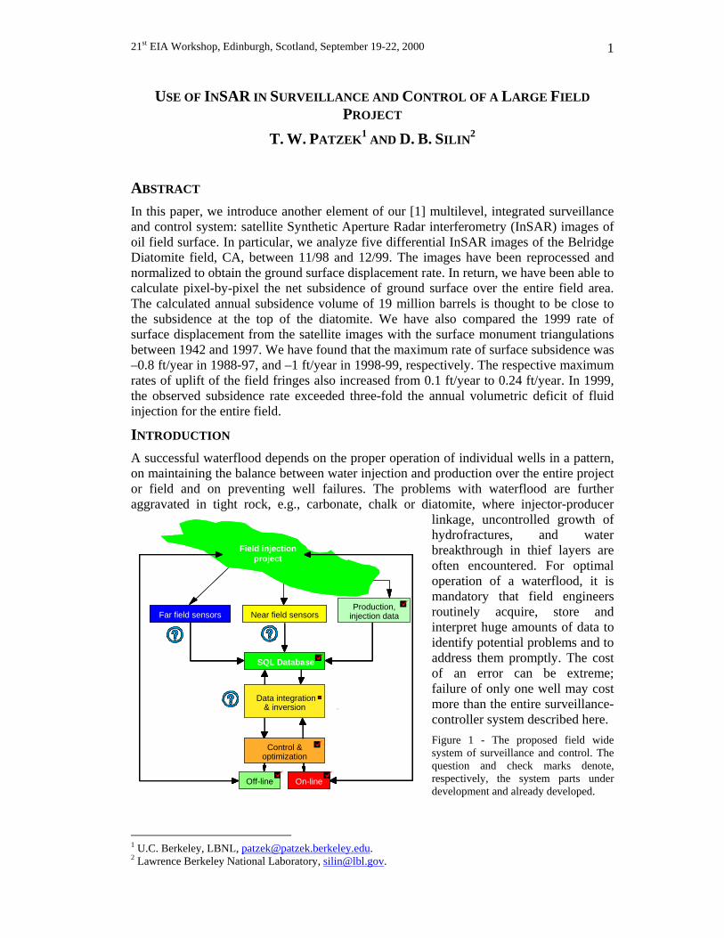
Figure 1 - The proposed field wide system of surveillance and control. The question and check marks denote, respectively, the system parts under development and already developed.

1 U.C. Berkeley, LBNL, [email protected]. 2 Lawrence Berkeley National Laboratory, [email protected].

Far field sensors Near field sensorsProduction,

injection data

SQL Database

Control & optimization

Data integration & inversion

Off-line On-line

Field injectionproject

Far field sensors Near field sensorsProduction,

injection data

SQL Database

Control & optimization

Data integration & inversion

Off-line On-line

Field injectionproject


As in preventive health care, it is important to diagnose the problems early and to apply the cure on time. Our solution is [1] to design a multilevel, integrated system of surveillance and control, which acquires and processes waterflood data, and helps field personnel make optimal decisions, Figure 1. Our systems for shallow oilfields (<9000 ft in depth) in arid surroundings will use Synthetic Aperture Radar interferograms (InSAR) acquired from satellites. In the last few years, InSAR has become a very attractive technique to obtain more information from SAR images [2], [3]. Both the amplitude of the signal and its phase are used. Usually, two SAR images of the same region are acquired with slightly different sensor positions, and coherently combined together. SAR interferometry can be performed either using data collected by repeat-pass or single-pass sensors. The former implies the same antenna is used twice while the latter requires two distinct antennas to be flown aboard the aircraft or satellite. This paper focuses on the ERS repeat-pass InSAR images acquired in 1998/99 by Atlantis Scientific, Inc., for the giant Belridge Diatomite field in California, U.S.A. ERS-1, a satellite carrying a space borne C-band SAR, was launched in July 1991, while ERS-2 was launched in April 1995. Both satellites were built by ESA3, are identical from the SAR point of view, and they acquire data over the Earth with incidence angles varying between 19 deg and 26 deg with slant-range pixel spacing set to 7.9 m for the Single Look Complex (SLC) product. In petroleum industry, a promising application of SAR interferometry is to generate time-lapse digital elevation maps (DEM) owing to the fact that the change of height information can be related with great precision to the phase difference between two SAR interferograms. The rate of surface displacement can then be combined with the overall volumetric balance of fluid injection to identify the areas with most imbalance and/or highest gas saturation. If information about vertical sweep by water is also available from cross-well images [4], then volumetric sweep can be estimated. This technique will be useful especially for relatively shallow waterfloods and very shallow steamfloods.

PROCESSING OF THE SAR DATA

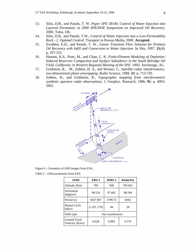
For a thorough review of the principles of imaging radar see [2], [5] and [6], and references therein. Briefly, imaging radar is an active illumination system, Figure 6, side-looking with respect to the vehicle's direction of travel. The brightness (amplitude, A) of a reflected radar echo that has been transmitted from an antenna mounted on an aircraft or spacecraft, backscattered from the surface of the Earth, and received a fraction of a second later by the same antenna, is measured and recorded to construct the image, Table 2- Table 5. Let us consider an image to be a set of values ( , )A x y , where the x-coordinate is in the direction of platform motion and the y-coordinate is in the direction of illumination. The value of y (related to the radar range) and its resolution is based on the arrival time of the echo and the timing precision of the radar, while the value of x (related to the radar azimuth) and its resolution depends on the position of the platform and the beam width of the radar. Since the beam-width is inversely related to antenna size, small (physically realizable) antennas tend to generate large footprints and their corresponding images have poor azimuthal resolution. Synthetic aperture radar (SAR) takes advantage of the Doppler history of the radar echoes generated by the forward motion of the vehicle

3 The European Space Agency.


to synthesize a large antenna, enabling high azimuthal resolution in the resulting image despite a physically small antenna. Even though a typical radar image displays only amplitude data, the aspect of SAR most important here is its coherence, i.e., retention of both amplitude and phase information in the radar echo during data acquisition and subsequent processing. The details of SAR interferometry are summarized in Appendix A. There, we examine estimation of topographic height from the differential range measured by two radar antennas looking at the same surface, followed by a discussion of changes in topography (surface displacement) based on range change in two or more successive SAR images. Interferometric processing of complex SAR data combines two single look complex (SLC) images4 into an interferogram. First, the two images are co-registered (aligned), and their amplitudes and phases are adjusted by interpolation. In the same step common band-filtering of the azimuth and range spectra can be conducted, in order to include only those parts of the spectra which are common to the two images, and thereby optimize the interferometric correlation and minimize the effects of the baseline geometry on the interferometric correlation. Then the two images are cross-correlated, i.e. the normalized complex interferogram is computed. The interferogram displays the phase difference information. The azimuth and range phase trends expected for a flat Earth are removed from the interferogram. From this “flattened” interferogram and the two registered intensity images the multi-look interferometric correlation and backscatter intensities are estimated. The interferogram phase is further “unwrapped” to solve for the integer number of wavelengths wrapped into it, and to obtain the absolute range.

APPLICATION TO BELRIDGE DIATOMITE

This paper is an initial attempt to bring together the satellite images of the field surface and the volumetric balance of injection and withdrawal. Obviously, more work needs to be done and our conclusions will be modified as our understanding of the correlation between surface displacement and waterflood performance improves. The late and middle Miocene diatomaceous oil fields in the San Joaquin Valley, California, are located in Kern County, some forty miles west of Bakersfield. An estimated original-oil-in-place in the Monterey diatomaceous fields exceeds 10 billion barrels and is comparable to that in Prudhoe Bay in Alaska. In Belridge, cyclic bedding of the diatomite is a well-documented phenomenon [7], attributed to alternating deposition of detritus beds, clay, and biogenic beds. The cycles span length-scales that range from a fraction of an inch to tens of feet, reflecting the duration of depositional phases from semi-annual to thousands of years. On a large scale, there are at least seven distinct oil producing layers with good lateral continuity within each layer, but little vertical continuity between adjacent layers. The diatomite is very porous (25-65 percent), rich in oil (35-70 percent), and nearly impermeable (0.1-10 millidarcy). The high porosity and oil saturation, together with large thickness (up to 1000 feet) and area translate into the gigantic oil-in-place estimates. To compensate for the low reservoir permeability, all wells in the diatomite are hydrofractured. A typical well has 2-8 fractures with a target fracture half-length of 150 feet. Wells are often spaced along lines following the maximum in-situ stress every 165

4 The images contain both the amplitude and phase information.


feet (1-1/4 acre), 82 feet (5/8 acre), or even smaller. Thousands of hydrofractures have been already induced and thousands more may be created as waterflood and steam drive projects on 5/8 acre or smaller spacing are being introduced. The injector hydrofractures in the shallow diatomite (600-1000 ft BGL) may link with the producers [8], and they grow [9-14].

Table 1 – Characteristic time of pressure diffusion in years for the South Belridge diatomite cycles at different injector-producer spacing; the hydraulic diffusivity data are from [15]

Cycle Diffusivitysq. ft/day 5/16-acre 5/8-acre 1-1/4 acre 2.5-acre

G 0.573 8 31 122 299 H 0.135 32 130 520 1268 I 0.045 97 390 1559 3805 J 0.425 10 41 165 403 K 0.919 5 19 76 186 L 0.426 10 41 165 402 M 0.26 17 67 270 659

Figure 2- Cumulative surface displacement between 1942-1988 and 1988-1997 in ft (left), and the mean annual subsidence rate in ft/year (right) in the Belridge Diatomite. The images have been constructed from the triangulated monument data provided by Aera Energy, LLC. The largest cumulative subsidence is about 16 ft, and that the maximum annual rate of subsidence quadrupled in the decade after 1988, i.e., after the installation and expansion of waterflood. Note that in the last decade a large-scale uplift of the fringes of the field was observed. The xy-coordinates are Easting and Northing in ft.

With reasonable estimates of the diatomite layer properties at South Belridge, Table 1, it may take hundreds of years to propagate pressure from an injector to a producer.


Consequently, waterflood projects that rely on water imbibition into the diatomite and avoid early water breakthrough may take over 100 years to complete. Conversely, aggressive water injection with early water breakthrough in few layers may fail to provide pressure support for the entire diatomite column and alleviate subsidence. Because of the slow propagation of pressure from the injectors and the simultaneous fluid withdrawal at the producers, subsidence has been a severe problem in Belridge [16]. As shown in Figure 2, the maximum rate of subsidence in the last decade can be 4 times higher than that experienced earlier. As of 1999, Figure 3, the rate of subsidence was still substantial, and was accompanied by gradual uplift of the field fringes. The InSAR images of South Belridge, Figure 3, provide wealth of high-resolution information about surface displacement compared with the old monument data. The rate of surface displacement can now be calculated in monthly intervals over the entire field. The resulting net subsidence can then be calculated over the entire field area, with a higher precision than ever before. Our analysis of the InSAR images shows that maximum annual rate of surface deformation increased in 1998/99 relative to 1988-1997.

Figure 3 – The current (11/98-12/99) rate of surface displacement above the Belridge diatomite from InSAR images. The rate in normalized to ft/month, so the scale becomes +0.24 to –1 ft/year when rescaled to the mean annual rate of displacement. The pair of interferograms between 03-14-99 and 08-01-99 is de-correlated because of the very large subsidence in the SW part of the field. The maximum subsidence rate is consistently higher than that between 1988 and 1997. The rate of uplift of the field fringes is double that in the prior decade.


In 1998/99, the overall net rate of surface subsidence in Belridge was relatively constant, amounting to about 19 million barrels, Figure 4. From the calculations by Hansen et al. [16], it follows that subsidence at the reservoir top is close to that at the surface. Therefore, we can assume that in Belridge the net reservoir-level compaction was at least 19 million barrels in 1999. Oil and water production rates as well as water injection rate in the Belridge diatomite are shown in Figure 5. The most striking feature of this plot is balance of annual injection and production since 1989 and a robust water response to the increased injection in 1995.

0

5

10

15

20

25

Nov-98 Jan-99 Mar-99 May-99 Jul-99 Sep-99 Nov-99

Cum

ulat

ive

subs

iden

ce, M

Mbb

Figure 4 – Current annual subsidence in Belridge calculated from InSAR images. The net surface subsidence, subsidence - uplift, was about 19 million barrels in 1999.

0

10,000,000

20,000,000

30,000,000

40,000,000

50,000,000

60,000,000

70,000,000

80,000,000

1977 1982 1987 1992 1997

Barr

els

per Y

ear

Oil

Water

Injection

Water+Oil

Figure 5- Annual production and injection rates in the Belridge diatomite. Globally, Belridge has always been on net withdrawal, although liquid production and injection rates were almost balanced in the last decade. Data source: CCCOGP, ftp://ftp.consrv.ca.gov/pub/oil/annual_reports/, 1999 data are from Aera Energy.

CONCLUSIONS

Our initial evaluation shows that the satellite Synthetic Aperture Radar interferograms (InSAR) are a unique source of detailed and precise information of surface displacement over a giant oil field, Belridge Diatomite, in California, U.S.A. Using time-lapse differential interferograms, we were able to calculate net subsidence of the ground in


Belridge. In 1999, the total subsidence was about 19 million barrels, a volume equal approximately to three times the annual injection deficit in Belridge. Further analysis is necessary to gain a more complete understanding of time evolution of waterfloods in Belridge.

ACKNOWLEDGEMENTS

This work was sponsored by the DOE ORT Partnership under Contract DE-ACO3-76FS0098 to the Lawrence Berkeley National Laboratory. Partial support was also provided by gifts from Chevron to UC Oil, Berkeley. We would like to thank Dr. Robert Lynch of Atlantis Scientific, Inc. who acquired and processed the satellite images. We would like to thank Aera Energy and Chevron for their support. Aera Energy has provided Berkeley with the satellite InSAR images, monument and GPS elevation data, as well as overall production and injection data. We would like to extend special thanks to Mr. David Mayer of Aera Energy for his help and patience.

REFERENCES

1. De, A., Silin, D. B., and Patzek, T. W. SPE 59295: Waterflood surveillance and supervisory control. in 2000 SPE/DOE Improved Oil Recovery Symposium. 2000. Tulsa, OK.

2. Bürgmann, R., Rosen, P. A., Fielding E. J., Synthetic Aperture Radar Interferometry to Measure Earth's Surface Topography and its Deformation. Ann. Rev. Earth Planet. Sci., 2000. 28: p. 169-209.

3. Borgeaud, M., and Wegmuller, U. On the Use of ERS SAR Interferometry for the Retrieval of Geo- and Bio-Physical Information. in ERS SAR Interferometry Workshop 1996. 1996. Remote Sensing Laboratories, University of Zurich.

4. Patzek, T.W., Wilt, M., and Hoversten, M.,. Paper SPE 59529, Using Crosshole Electromagnetics (EM) for Reservoir Characterization and Waterflood Monitoring. in 2000 SPE Permian Basin Oil and Gas Recovery Conference. 1999. Midland, TX.

5. Jensen, H.L., Graham, L. J., Pocello, L. J., and Neith E. N., Side-looking airborne radar. Scientific American, 1977. 237: p. 84-95.

6. Elachi, C., Spaceborne imaging radar: geologic and oceanographic applications. Science, 1980. 209: p. 1073-1082.

7. Schwartz, D.E., Characterizing the Lithology, Petrophysical Properties, and Depositional Settings, South Belridge Field, Kern County, CA., in Studies of the Geology of the San Joaquin Basin, S.A. Graham, and Olson, H. C., Editor. 1988, The Pacific Section Society of Economic Paleontologists and Mineralogists: Los Angeles, CA.

8. Patzek, T.W. Paper SPE 24040, Surveillance of South Belridge Diatomite. in Proceedings of the Western Regional SPE Meeting. 1992. Bakersfield, CA.

9. Ilderton, D., Patzek, T. W., Rector, J. W., and Vinegar, H. J., Microseismic Imaging of Hydrofractures in the Diatomite. SPE Formation Evaluation J., 1996(March): p. 46-54.

10. Kovscek, A.R., Johnston, M., and Patzek, T. W., Interpretation of Hydrofracture Geometry Using Temperature Transients I: Model Formulation and Verification. In Situ, 1996. 20(3): p. 221-250.

11. Kovscek, A.R., Johnston, M., and Patzek, T. W., Interpretation of Hydrofracture Geometry Using Temperature Transients II: Asymmetric Hydrofractures. In Situ, 1996. 20(3): p. 251-289.

12. Patzek, T.W., and Silin, D. B., Control of Water Injection into a Low-Permeability Rock. 1. Hydrofracture Growth. Transport in Porous Media, 2000. Accepted.


13. Silin, D.B., and Patzek, T. W. Paper SPE 58140, Control of Water Injection into Layered Formation. in 2000 SPE/DOE Symposium on Improved Oil Recovery. 2000. Tulsa, OK.

14. Silin, D.B., and Patzek, T.W., Control of Water Injection into a Low-Permeability Rock - 2. Optimal Control. Transport in Porous Media, 2000. Accepted.

15. Zwahlen, E.D., and Patzek, T. W., Linear Transient Flow Solution for Primary Oil Recovery with Infill and Conversion to Water Injection. In Situ, 1997. 21(4): p. 297-331.

16. Hansen, K.S., Prats, M., and Chan, C. K. Finite-Element Modeling of Depletion-Induced Reservoir Compaction and Surface Subsidence in the South Belridge Oil Field, California. in Western Regional Meeting of the SPE. 1993. Anchorage, AL.

17. Goldstein, R., . M., Zebker, H. A., and Werner, C., Satellite radar interferometry: two-dimensional phase unwrapping. Radio Science, 1988. 23: p. 713-720.

18. Zebker, H., and Goldstein, R., Topographic mapping from interferometric synthetic aperture radar observations. J. Geophys. Research, 1986. 91: p. 4993-5001.

Figure 6 – Geometry of SAR images from ESA.

Table 2 – Orbit parameters from ESA

Orbit ERS-1 JERS-1 RadarSat

Altitude (Km) 785 568 793-821

Inclination (degrees) 98.516 97.662 98.594

Period (s) 6027.907 5799.72 6042

Repeat Cycle(days) 3, (35, 176) 44 24

Orbit type Sun synchronous

Ground Track Velocity (Km/s)

6.628 6.883 6.576


Table 3 – SAR instrument parameters from ESA

Instrument ERS-1 JERS-1 RadarSat

Frequency C-Band (5.3 GHz)

L-Band (1.275 GHz)

C-Band (5.3 GHz)

Wavelength (cm) 5.66 23.5 5.66

Pulse Repetition Frequency (Hz) 1640-1720 1505.8-1606 1270-1390

Pulse Length (s) BW (MHz)

37.1 15.5

35 15

42 11.6, 17.3, 30

Polarization VV HH HH

Antenna Size (L x W m) 10 x 1 11.9 x 2.4 15 x 1.5

Peak Power (kW) 4.8 1.3 5

Average Power (W) 300 71 300

Noise Equivalent (dB) -18 -20.5 -21

Table 4 – Image parameters from ESA

Image ERS-1 JERS-1 RadarSat

Swath Width (km) 100 75 50, 100, 150, 500

Max Resolution (Range x Azimuth m)

12.5 x 12.5 7 x 7 10 x 10

Resolution (No looks) 30 (4) 18 (3) 28 x 30 (4)

Table 5 – System parameters from ESA

System ERS-1 JERS-1 RadarSat

Look Angle (Degrees) Right 20.335 Right 35.21 Right, Left 20 - 50

Incidence Angles. Mid (Degrees) 19.35-26.60, 23 16.14-41.51, 38.91 22.64-59.56, 45.12

Footprint (Range x Azimuth km) 80 x 4.8 70 x 14 50-150 x 4.3

APPENDIX A – SURFACE TOPOGRAPHY FROM SAR

Single-pass InSAR. Consider two radar antennas, 1A and 2A , simultaneously scanning

the Earth surface and separated by the baseline vector B

of length B and angle , with respect to horizontal, Figure 7. In this example, the first antenna transmits and receives the radar signal, while the second one only receives. The phase difference between backscattered signal received by the two antennas is a function of viewing geometry and the elevation of point z above the reference surface 0H . If the viewing geometry is known with sufficient accuracy, then the surface topography z(y) can be calculated from the phase measurement to a precision of several meters, assuming that we can solve (“unwrap”) for the 2 ambiguity inherent in phase measurements. From geometry it follows that

1( ) cosz y H R (1.1)

where is the “look” angle of the radar with respect to vertical, and 1R is the range.


From elementary trigonometry

2 2 2 22 1 1 1

2 221

1

( ) 2 (sin cos cos sin cos )

2sin( ) , when 2

2

R R dR R B R B

R dR dR B

R B

(1.2)

where is the angle between the zy-plane in Figure 7 and plane 1 2A A C , measured along

a horizontal plane through point 1A . For simplicity, we will assume here that this angle is small5. The two images are co-registered, i.e., aligned and rescaled, and the first one is multiplied by the complex conjugate of the second one. The result is an interferogram with the representation6 1 2( ) 2

1 2i iA A e A e . The fractional phase difference between

the two antennas scales as

2

dR

, (1.3)

where is the signal wavelength. Note that the fractional phase [0,2 ] leads to ambiguity in range. Additional techniques, such as “phase unwrapping,” Figure 8, are used to solve for the integer number of wavelengths to obtain absolute range [17].

1A

2A

( )z y

y

z

H 1R

2 1R R dR

C

B

1re

1A

2A

( )z y

y

z

H 1R

2 1R R dR

C

B

1re

Figure 7 – Imaging geometry for SAR interferometry. A1 and A2 are two radar antennas viewing the same surface simultaneously (spatial separation), or a single antenna viewing the same surface on two separate

passes (temporal separation). B

is the baseline vector, R1 is the range of the first antenna, is the look

angle of the radar with respect to vertical, is the angle of B

with respect to horizontal, and r

e

is the unit

vector along the line-of-sight R.

5 This assumption is made in most literature derivations. It is not true for single-pass data acquisition. 6 The actual generation of interferograms is much more sophisticated, cf. [2].


-

2

3

Figure 8 – SAR interferogram phase unwrapping.

Equations (1.1) - (1.3) can now be combined to express the unknown topography z(y) in terms of the observed phase difference and the radar system parameters:

2

11 2( ) cos2 sin( )

2

Bz y H

B

(1.4)

Height estimates are averaged over a surface resolution element of the radar image (picture element or pixel), typically tens of meters of diameter. Repeat-pass InSAR. Now we consider a single-antenna SAR satellite that revisits the same area after several days or weeks. If there has been no significant change in the surface between the two acquisitions, we can perform essentially the same analysis as above and recover the same level of detail. In this case, we rewrite Eq. (1.3) as

4dR

, (1.5)

or 2 times the round-trip distance difference in wavelengths. Rearranging Eq. (1.2)2 and neglecting the small 2dR gives:

2

1

sin( )2

BdR B

R (1.6)

For spaceborne geometries, we can make the parallel ray approximation [18] and ignore the last term on the right side of Eq. (1.6):

sin( )dR B B (1.7)

where B is the projection of the baseline onto the line of sight.


Can we still recover topography if the surface has changed? It depends. If the relative positions of the radar scatterers within each pixel change more than one wavelength, we cannot perform the pixel-by-pixel comparison between the two images. Now consider a case, where the surface displacement is coherent on a large-scale, i.e., across several pixels. In other words, the relative position of the radar scatterers does not change, but the ground moves up or down across several pixels. Now we can perform a phase comparison between the two images. The differential phase contains information about the radar beam range change, precise to a fraction of a radar wavelength, or about 1 cm for the C-band systems. To measure the surface displacement with this precision requires an accurate Digital Elevation Model (DEM) of the surface and very precise knowledge of the satellite positions. Differential interferograms. If the second interferogram is acquired over the same area, sharing the orbit with the first pair so that both 1R and are constant, we still can compare the phases of both interferograms. The second interferogram is acquired with a different baseline vector: ( , )B . Combining Eqs (1.5) and (1.7) we obtain

4

.B

(1.8)

Therefore the ratio of the two phase-differences,

B

B

, (1.9)

is equal to the ratio of the parallel components of the baselines, and it is independent of topography. Now consider two interferograms acquired over the same region as before, but at two different times, so that ground deformation caused by subsidence or uplift has displaced many of the pixels in the primed interferogram in a coherent manner. In addition to the dependence on topography, there is now an additional phase change caused by the ground displacement along the radar line-of-sight, R :

4B R

(1.10)

The ground surface displacement R adds to the topographic phase term and may cause interpretation problems. However, if the data in the first interferogram is scaled properly and subtracted from the second one, one obtains a solution that depends only on the displacement R :

4B

RB

(1.11)

Since the quantity on the left is determined only by the phase differences in the respective interferograms and the orbit geometry, the line-of-sight displacement component R is measurable at each pixel.

use of insar in surveillance and control of … of insar in... · 21st eia workshop, edinburgh,...

Documents