use of particle ﬁlters in an active control algorithm for...

ARTICLE IN PRESS

JOURNAL OFSOUND ANDVIBRATION

0022-460X/$ - s

doi:10.1016/j.js

�CorrespondE-mail addr

Journal of Sound and Vibration 306 (2007) 111–135

www.elsevier.com/locate/jsvi

Use of particle filters in an active control algorithm for noisynonlinear structural dynamical systems

R. Sajeeb, C.S. Manohar, D. Roy�

Structures Lab, Department of Civil Engineering, Indian Institute of Science, Bangalore 560012, India

Received 10 October 2006; received in revised form 15 May 2007; accepted 19 May 2007

Available online 6 July 2007

Abstract

The problem of active control of nonlinear structural dynamical systems, in the presence of both process and

measurement noises, is considered. The focus of the study is on the use of particle filters for state estimation in feedback

control algorithms for nonlinear structures, when a limited number of noisy output measurements are available. The

control design is done using the state-dependent Riccati equation (SDRE) method. The stochastic differential equations

(SDEs) governing the dynamical systems are discretized using explicit forms of Ito–Taylor expansions. The Bayesian

bootstrap filter and that based on sequential important sampling (SIS) are employed for state estimation. The simulation

results show the feasibility of using particle filters and SDRE techniques in control of nonlinear structural dynamical

systems.

r 2007 Elsevier Ltd. All rights reserved.

1. Introduction

The concept of active structural control, since its introduction in 1972 [1], has been extensively used forcontrol of civil engineering structures subjected to dynamic loads. The ability of the actively controlledstructures to adapt themselves to the frequency characteristics of the excitation [2] makes it very attractive inthe field of earthquake engineering. Excellent surveys of the state-of-the-art techniques and developments inthis field are available in Refs. [3,4]. Most of the research in this field deals with control of linear structures.The real engineering structure is, however, typically nonlinear and therefore a successful implementation ofcontrol systems demands control algorithms which are capable of handling structural nonlinearity.

Different control schemes, such as feedback linearization, gain scheduling, sliding mode control and backstepping control are used in practice for control of nonlinear systems. The details of these methods can befound in Refs. [5,6]. A recently developed technique that has shown considerable promise is the nonlinearextension to the linear quadratic regulator (LQR) problem, called the state-dependent Riccati equation(SDRE) method. An overview of this method is available in Ref. [7]. In the SDRE method, the equations ofmotion are represented in a linear-like form, called the state-dependant coefficient (SDC) form thatcorresponds to the system matrices expressed explicitly as functions of the current state. A standard LQR

ee front matter r 2007 Elsevier Ltd. All rights reserved.

v.2007.05.043

ing author. Tel.: +9180 2293 3129; fax: +9180 2360 0404.

ess: [email protected] (D. Roy).

www.elsevier.com/locate/jsvi

dx.doi.org/10.1016/j.jsv.2007.05.043

mailto:[email protected]

ARTICLE IN PRESSR. Sajeeb et al. / Journal of Sound and Vibration 306 (2007) 111–135112

problem can then be solved over each time step to design the state feedback control law. Indeed, most of thedynamical systems of engineering interest allow a direct parameterization of the equations of motion in theSDC form. However, systems, which do not admit a direct parameterization, may also be handled [8]. Theparameterization is not unique and the control law is sub-optimal. It has been shown that there exists arepresentation such that the SDRE feedback produces the optimal control law [9]. The stability of thefeedback control law resulting from the SDRE method is well studied [9–13]. Global asymptotic stability of ageneral nonlinear system can be achieved by tuning the weighing parameters of the cost function as function ofstates [10]. Although computationally intensive, the SDRE technique is found to be practicable for real-timecontrol applications [11,14]. The availability of fast and efficient numerical algorithms for solving the SDREmakes the SDRE method suitable for field applications of real-time control systems [15]. The SDRE-basedcontrol design has received wide acceptance among researchers in different fields like, aerospace engineering[16–20], robotics [14] and bio-medical engineering [21]. However, the potential of this method in structuralcontrol problems appears not to have been explored yet.

To develop a control algorithm, to be implemented successfully in structural engineering applications, onehas to consider important issues such as limitations of the mathematical model, and the difficulty in measuringall the state variables. Due to the size and complexity of many structures, mathematical models may notrepresent all aspects of their behavior. The uncertainty so introduced in the model (process noise) assumesgreat importance in control design, since the performance of the control design depends on the accuracy of thepredicted response. Although considerable literature is available on the control of nonlinear structural systems[22–34], uncertainties in the model have not been generally considered except in a few studies [28,32–34].Studies reported in Refs. [29–31] refer to the optimal control of nonlinear systems of interest in structuralengineering. However, stochastic optimal control of nonlinear systems has been considered only in a very fewstudies [32–34]. A comprehensive review on the recent advances in the control of nonlinear stochastic systemsis available in Ref. [35]. One important aspect of considerable relevance in structural control is the non-availability of the full states of the system. It is seldom feasible to measure all the states of the system that arerequired for the design of the control system. Measurements of a very few states, often contaminated by noise,are usually available. If the effect of noise is ignored, one can still design a control system, using the concept ofdirect output feedback control design [36]. But the resulting control will not be as effective as the statefeedback control. A practical strategy for designing an efficient control system using the available noisymeasurements would be to use a filter for estimating the states from the limited available responses and designa state feedback control via the estimated states. The separation principle in control theory allows one tohandle the control design and filtering separately. Though the theory holds for linear systems [37] and possiblyfor a class of nonlinear systems [38–40], a generally applicable form of such a theory is not yet available fornonlinear systems [5]. It is nevertheless desirable to design the controller and state estimator separately, even inthe absence of a rigorously established separation principle [41,42]. In the present study, the filtering andcontrol strategies are designed separately with the implicit assumption that a separation theory holds.

One has to use an appropriate filter/state estimator to estimate the states that in turn serve as input to thefeedback controller. For a linear system with Gaussian additive noises, the classical Kalman filter provides theoptimal state estimator. For nonlinear state estimation, there are two main classes of methods, viz., those basedon extended Kalman filter (EKF) and its variants [43,44], and, those based on Monte Carlo simulations,popularly known as the particle filters [45–50]. The current practice for estimating dynamic states of a nonlinearsystem, required for control applications, is to use the EKF [41,42,51]. The EKF, which uses a local linearizationaround the current state, does not account for the non-Gaussian nature of nonlinear system states, and, therefore,can approximately capture only the first two moments of the conditional probability density function (pdf) of thestate. This may be contrasted with particle filters, wherein the conditional pdf is directly updated through a set ofrandom particles with associated weights. Therefore, unlike the EKF, particle filters are far more versatile inhandling system nonlinearity, non-Gaussian nature of response and even non-Gaussian nature of noises.Different versions of particle filters are discussed in the literature. Density-based Monte Carlo filter, Bayesianbootstrap filter and sequential important sampling (SIS)-based filter are some of them. A summary of thedevelopment of these filters can be found in Refs. [52,53]. Particle filters provide powerful tools in stateestimation, system identification and control [54]. Recently, the potential of this technique has been demonstratedfor system identification of nonlinear structural dynamical systems [53].

ARTICLE IN PRESSR. Sajeeb et al. / Journal of Sound and Vibration 306 (2007) 111–135 113

To the best of the authors’ knowledge, the applicability of particle filters for state estimation in nonlinearstructural control applications has not been explored yet. In the present work, we use particle filters for stateestimation and control of a few typically nonlinear oscillators of interest in structural engineering. Theexample problems include a Duffing oscillator, a Van der Pol oscillator, and a three degree-of-freedom (3-dof)spring mass system with bilinear stiffness characteristics. The control strategy, designed using the SDREmethod, uses the states estimated from a limited number of noisy measurements available. The governingstochastic differential equations (SDEs) of these oscillators are numerically integrated using explicit marchingschemes based on the Ito–Taylor expansion, for processing in the filtering algorithm. The simulations areclearly indicative of the feasibility of particle filters and SDRE technique in control of nonlinear structuraldynamical systems.

2. Problem description

By way of a general framework, consider a nonlinear dynamical system in the state space form as_x ¼ f ðx; uÞ, where xðt; uÞ : <� <nu ! <nx represents the state vector and u 2 <nu is the control force acting onthe system. For notational convenience, we will often write x(t, u) as x(t) by dropping the argument u. Theuncertainty in the system, arising from errors due to modeling and other sources, is assumed to admit arepresentation through Gaussian white noise processes. The governing equations therefore take the form of asystem of SDEs. The white noise process, which is defined as the formal derivative of the Weiner process, onlyexists as a measure and not as a valid mathematical function. Hence, the governing SDEs are expressed in thefollowing incremental form:

dxðtÞ ¼ ~F ½xðtÞ; uðtÞ; t�dtþ ~G½xðtÞ; t�dBI ðtÞ; xð0Þ ¼ x0. (1)

Here, BI ðtÞ 2 <mI is a standard vector Brownian motion process; ~F : <nx �<nu �<! <nx is the drift vector

function, ~G : <nx �<! <nx�mI is the diffusion coefficient matrix and x0 ¼ x(t0) is the initial condition vector,which may be deterministic or random with a known description. If one directly measures the state at a set ofdiscrete time instants ftkg

nk

k¼1, the measurement equation may be formally expressed as

yk ¼ HkðxkÞ þ xk; k ¼ 1; 2; . . . ; nk. (2)

Here, xk 2 <ny formally represents the vector of measurement noise. The objective is to determine the

control force u(t) so that a performance index of the form

J ¼ limtf!1

1

tf

E

Z tf

0

L½xðtÞ; uðtÞ; t�dt

� �(3)

is minimized. Here E[ � ] represents the mathematical expectation operator and L[ � ] is a cost function whosedefinition would be made more precise later in the paper.

Since the focus of the present study is to demonstrate the use of particle filters in a structural controlalgorithm, the problem described through Eqs. (1)–(3) is not directly attempted here.

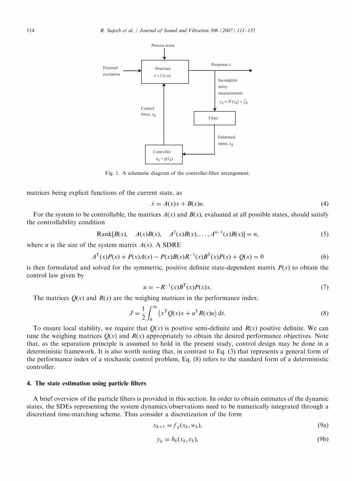
Assuming that the separation principle holds, one may tackle the output feedback control problem in twosteps: (1) design a state feedback control law, assuming that the state x(t) is available and (2) design a filter andreplace x with the estimate x in the control law. Though, there is no general separation principle available fornonlinear systems, its validity is often assumed for all practical purposes. The controller-filter arrangement isschematically shown in Fig. 1. In the present study, we assume that the separation principle holds and designthe controller and state estimator separately. A sub-optimal control law is designed using the SDRE methodand the state estimation is done using a particle filter.

3. The control design using the SDRE method

The SDRE method, which is a nonlinear extension of the classical LQR control law, has received wideacceptance for control of nonlinear structures in recent years [14,16–21]. The details of this method can befound in Refs. [7,8]. The SDRE control design procedure is briefly outlined here. Here the governing equationof the nonlinear system _x ¼ f ðx; uÞ is represented in a linear-like form, i.e., the SDC form with the system

ARTICLE IN PRESS

Response x Structure

Filter

External

excitation

Incomplete

noisy

measurements

Controller

Control

force, uk

x = f (x,u).

Estimated

states, xk

Process noise

ˆ

uk = g(xk)ˆ

yk = H [xk] + �k

Fig. 1. A schematic diagram of the controller-filter arrangement.

R. Sajeeb et al. / Journal of Sound and Vibration 306 (2007) 111–135114

matrices being explicit functions of the current state, as

_x ¼ AðxÞxþ BðxÞu. (4)

For the system to be controllable, the matrices A(x) and B(x), evaluated at all possible states, should satisfythe controllability condition

Rank½BðxÞ; AðxÞBðxÞ; A2ðxÞBðxÞ; . . . ;An�1ðxÞBðxÞ� ¼ n, (5)

where n is the size of the system matrix A(x). A SDRE

ATðxÞPðxÞ þ PðxÞAðxÞ � PðxÞBðxÞR�1ðxÞBTðxÞPðxÞ þQðxÞ ¼ 0 (6)

is then formulated and solved for the symmetric, positive definite state-dependent matrix P(x) to obtain thecontrol law given by

u ¼ �R�1ðxÞBTðxÞPðxÞx. (7)

The matrices Q(x) and R(x) are the weighing matrices in the performance index:

J ¼1

2

Z 10

xTQðxÞxþ uTRðxÞu� �

dt. (8)

To ensure local stability, we require that Q(x) is positive semi-definite and R(x) positive definite. We cantune the weighing matrices Q(x) and R(x) appropriately to obtain the desired performance objectives. Notethat, as the separation principle is assumed to hold in the present study, control design may be done in adeterministic framework. It is also worth noting that, in contrast to Eq. (3) that represents a general form ofthe performance index of a stochastic control problem, Eq. (8) refers to the standard form of a deterministiccontroller.

4. The state estimation using particle filters

A brief overview of the particle filters is provided in this section. In order to obtain estimates of the dynamicstates, the SDEs representing the system dynamics/observations need to be numerically integrated through adiscretized time-marching scheme. Thus consider a discretization of the form

xkþ1 ¼ f kðxk;wkÞ, (9a)

yk ¼ hkðxk; vkÞ, (9b)


where f k : <nx �<nw !<nx is a nonlinear function of the state xk 2 <

nx (with the subscript k denoting thetime instant tk), hk : <

nx �<nv ! <ny is a linear/nonlinear function of the state, wk 2 <nw and vk 2 <

nv arezero-mean noise variables independent of current and past states and yk 2 <

ny is the instantaneousmeasurement vector. Since the vector sequence xk is derived through a strong discretization of the governingSDEs, it follows that xk possesses the strong Markov property and that the conditional pdfs p(xkjxk�1) andp(ykjxk) are deducible from Eq. (9). For convenience, we introduce the following notations: x0:k:¼fxig

ki¼0 and

y1:k:¼fyigki¼1. The objective is to determine the conditional pdf, p(x0:kjy1:k), which represents the pdf of the

discretized state vectors conditioned on the observations available up to time tk.More specifically, we need to obtain the marginal pdf p(xkjy1:k), known as the filtering density, to estimate

such statistical properties as conditional mean xk and conditional covariance Sk given by

xk ¼ E½xkjy1:k� ¼

Zxkpðxkjy1:kÞdxk, (10a)

Sk ¼ E½ðxk � xkÞðxk � xkÞT� ¼

Zðxk � xkÞðxk � xkÞ

Tpðxkjy1:kÞdxk. (10b)

The integrals in Eq. (10) are multidimensional in nature and their analytical evaluations are generally notpossible. However, when the process and measurement equations are linear and the noises are Gaussian andadditive, the Kalman filter provides the exact solution. For a more general case, a formal solution may bederived as follows [45]:

pðxkjy1:k�1Þ ¼

Zpðxk;xk�1jy1:k�1Þdxk�1 ¼

Zpðxkjxk�1Þpðxk�1jy1:k�1Þdxk�1. (11)

This equation represents the prediction equation. When the measurement vector yk becomes available, onecan derive the updation equation as follows:

pðxkjy1:kÞ ¼pðxk; y1:kÞ

pðy1:kÞ¼

pðxk; yk; y1:k�1Þ

pðyk; y1:k�1Þ¼

pðykjxkÞpðxkjy1:k�1Þ

pðykjy1:k�1Þ. (12)

Using the identity pðykjy1:k�1Þ ¼R

pðxk; ykjy1:k�1Þdxk ¼R

pðykjxkÞpðxkjy1:k�1Þdxk, the updation equationmay further be expressed as

pðxkjy1:kÞ ¼pðykjxkÞpðxkjy1:k�1ÞR

pðykjxkÞpðxkjy1:k�1Þdxk

. (13)

Eqs. (11) and (13) constitute the formal solution to the estimation problem. The general principle of theparticle filters is to use Monte Carlo simulation strategies to approximately obtain the above integrals.Different versions of particle filters such as density filter [46], Bayesian bootstrap filter [45], and SIS filters[48,49,52] are available in the literature. The density filter does not use a resampling scheme and hence, after afew time steps, the effective sample size reduces. Both Bayesian bootstrap filter and filter based on SIS densityfunction uses some resampling strategies so that the samples get concentrated near regions of high probabilitydensities. In the present study, we mainly employ the Bayesian bootstrap filter for state estimation owing to itssimplicity and computational ease. However, we also use the filter based on SIS for comparison.

The formulation of the Bayesian bootstrap filter is based on an earlier result by Smith and Gelfand [55].This result can be stated as follows. Let fx�kðiÞg

Ni¼1 be samples available from a continuous density function

G(x) (where the argument ‘i’ within the inner parenthesis represents the ith event). Moreover, suppose that weneed samples from the pdf proportional to L(x)G(x), where L(x) is a known function. Then the theorem statesthat samples drawn from a discrete distribution over fx�kðiÞg

Ni¼1 with probability mass function

Lðx�kðiÞÞ.PN

j¼1Lðx�kðjÞÞ on x�kðiÞ tends in distribution to the required density as N tends to infinity. The

algorithm for implementing the filter is as follows:

1.
Set k ¼ 0. Draw sample fx�0ðiÞgNi¼1 from the pdf p(x0) and fw0ðiÞg
Ni¼1 from the pdf p(w) of the noise.

2.
Using the process Eq. (9a), obtain fx�kðiÞgNi¼1, k40, recursively..P
3.
When yk arrives, find pðykjx�i;kÞ and define qi ¼ pðykjx
�kðiÞÞ

Nj¼1pðykjx

�kðjÞÞ


4.
Define the probability mass function P½xkðiÞ ¼ x�kðiÞ� ¼ qi and generate samples fx�kðiÞgNi¼1 from this discrete
distribution. P
5. Estimate the conditional mean xk ffi ð1=NÞ
Ni¼1xkðiÞ and conditional covariance Sk ffi ð1=ðN � 1ÞÞPN

i¼1ðxkðiÞ � xkÞðxkðiÞ � xkÞT. The diagonal elements of Sk represent the variance associated with the

estimated states.
6. With k replaced by k+1, repeat steps 2 through 5 till the terminal time is reached.
Using the result by Smith and Gelfand, if G(x) is identified as p(xkjy1:k�1) and L(x) as p(ykjxk), one can seefrom the updation Eq. (14) that the samples fxkðiÞg

Ni¼1, drawn in step 4 above, are approximately distributed as

per the pdf p(xkjy1:k). In other words, the samples from the initial pdf p(x0) are propagated through the processequation and updated to represent samples from the filtering density.

If one uses the SIS filter, the estimate xk may be obtained by rewriting Eq. (10a) as

xk ¼

Zxk

pðxkjy1:kÞ

pðxkjy1:kÞpðxkjy1:kÞdxk ¼

Zxkw�ðxkÞpðxkjy1:kÞdxk ¼ Ep½xkw�ðxkÞ�, (14)

where Ep[ � ] stands for the expectation operator defined with respect to the pdf p(xkjy1:k) andw�ðxkÞ ¼ pðxkjy1:kÞ=pðxkjy1:kÞ. Obtaining the optimal importance sampling density function is not an easytask. However, when the process and measurement equations assume the form

xk ¼ f ðxk�1Þ þ vk; vk�N½ 0nv�1 Sv �, (15a)

yk ¼ Cxk þ wk; wk�N½ 0nw�1 Sw � (15b)

the optimal importance density function is shown to be a normal density function with mean mk andcovariance S given by

mk ¼ S S�1v f ðxk�1Þ þ CTS�1w yk

� �, (16a)

S�1 ¼ S�1v þ CTS�1w C. (16b)

When the effective sample size at any time instant falls below a threshold (Nthres), a resampling is performedto counter an impoverishment of samples. The algorithm for implementing the SIS filter is available in Refs.[49,52,53] and is skipped here for conciseness.

Theoretically, the estimate through the particle filter approaches the exact solution, as the number ofsamples N tends to infinity. It is therefore of interest to study the performance of the particle filter withdifferent sample sizes, especially for a linear system with Gaussian additive noises—a problem for which theexact solution is available through the Kalman filter. For a linear single degree of freedom (sdof) systemsubjected to a harmonic load, the variance associated with the estimates of velocity using Kalman filter andparticle filter (bootstap filter) with different ensemble sizes is shown in Fig. 2; the caption to this figureprovides the details of the system parameters considered. It is readily observable that the particle filter estimateapproaches the Kalman filter estimate as N increases.

5. The discretization of the system/observation equations

5.1. The discretization

The governing SDEs for the system/observations need to be discretized and brought to a form consistentwith Eqs. (9a) and (9b) and this enables further processing with the filtering algorithm. Just as a time-marchingalgorithm for a deterministic ODE is often derived using variations of a Taylor expansion, the SDEs maysimilarly be discretized using the stochastic Taylor (Ito–Taylor) expansion [56,57]. Details of Ito–Taylorexpansion and related concepts of stochastic calculus may be found in Refs. [53,56–58]. However, a briefoverview of the stochastic Taylor expansion is provided in the Appendix.

In the present study, we consider three nonlinear oscillators, namely, two sdof and a 3-dof oscillators. Whilethe sdof oscillators are the Duffing oscillator with a cubic stiffness term and the Van der Pol (VDP) oscillator

ARTICLE IN PRESS

Fig. 2. Performance of particle filter with different sample size. Here, a linear sdof system given by m €xþ c _xþ ax ¼ P0 cos lt is

considered. Initial condition: xð0Þ ¼ _xð0Þ ¼ 0. System parameters are: m ¼ 1 kg, c ¼ 0.5N s/m, a ¼ 10 N/m, P0 ¼ 5 N and l ¼ 5 rad/s.

Process noise parameter s ¼ 0.05P0 and standard deviation of measurement noise is 0.25. The filter estimates the states x1 (displacement)

and x2 (velocity) from the noisy measurement of x2.

R. Sajeeb et al. / Journal of Sound and Vibration 306 (2007) 111–135 117

with a nonlinear damping term, the nonlinearity in the 3-dof oscillator arises due to bilinear springs (Fig. 3).The forces u1(t), u2(t) and u3(t) acting in the model may be interpreted as control forces. The governingequations of motion of the sdof Duffing and VDP oscillators, both subjected to support motions, are,respectively, of the following forms:

m €xþ c _xþ axþ bx3 ¼ uðtÞ �m €xg; xð0Þ ¼ x0; _xð0Þ ¼ _x0, (17)

m €x� mð1� x2Þ _xþ ax ¼ uðtÞ �m €xg; xð0Þ ¼ x0; _xð0Þ ¼ _x0, (18)

where u(t) is the control force and x is the relative displacement of the mass point with respect to the support.Referring to Fig. 3(a), the equations of motion of the 3-dof spring-mass system, again under support motion,may be expressed as

m1 €x1 þ ðc1 þ c2Þ _x1 � c2 _x2 þ fs1ðx1Þ þ fs2ðx1 � x2Þ ¼ �m1 €xg þ u1ðtÞ, (19a)

m2 €x2 � c2 _x1 þ ðc2 þ c3Þ _x2 � c3 _x3 þ fs2ðx2 � x1Þ þ fs3ðx2 � x3Þ ¼ �m2 €xg þ u2ðtÞ, (19b)

m3 €x3 � c3 _x2 þ c3 _x3 þ fs3ðx3 � x2Þ ¼ �m3 €xg þ u3ðtÞ (19c)

with initial conditions x1(0) ¼ x10, x2(0) ¼ x20, x3(0) ¼ x30, _x1ð0Þ ¼ _x10, _x2ð0Þ ¼ _x20 and _x3ð0Þ ¼ _x30. x1, x2

and x3 are, respectively, the relative displacements of the mass points m1, m2 and m3 with respect to thesupport.

The SDEs corresponding to the Duffing oscillator (Eq. (17)), after incorporating the process noise, may beexpressed in the following incremental form:

dx1 ¼ x2 dt, (20a)

dx2 ¼1

m�ax1 � bx3

1 � cx2 þ uðtÞ� �

� €xg

� �dtþ sd dB1. (20b)

ARTICLE IN PRESS

m1

m1x1

c1(x1)

m2 m3

c1

m1

x1(t)

c2

m2 m3

c3

u1(t)

u1(t) u2(t)u3(t)

x2(t)

u2(t)

x3(t)

u3(t)

xg(t)

1

�

�1

xy

-xy

�1, �1 �2, �2 �3, �3

fs1(x1)fs2(x1 - x2)

c2(x1 - x2). . .

fs3(x2 - x3)

c3(x2 - x3). .

fs3(x3 - x2)

c3(x3 - x2). .

c2(x2 - x1). .

fs2(x2 - x1)..

m2x2..

m3x3..

Sp

rin

g F

orc

e (

fs)

Extension (x)

Fig. 3. (a) 3-dof spring–mass system with bilinear spring (x1, x2 and x3 represent the relative displacement with respect to the support) and

(b) force-displacement relation of the bilinear spring.


For the VDP oscillator, the SDEs in an incremental form are given by

dx1 ¼ x2 dt, (21a)

dx2 ¼1

m½ð�ax1 þ mð1� x2

1Þx2 þ uðtÞ� � €xg

� �dtþ sv dB1. (21b)

Similarly, the SDEs representing the 3-dof spring-mass system are

dx1 ¼ x4 dt, (22a)

dx2 ¼ x5 dt, (22b)

dx3 ¼ x6 dt, (22c)

dx4 ¼ �1

m1½ðc1 þ c2Þx4 � c2x5 þ fs1ðx1Þ þ fs2ðx1 � x2Þ� � €xg þ

u1ðtÞ

m1

� �dtþ s1 dB1, (22d)

dx5 ¼ �1

m2½�c2x4 þ ðc2 þ c3Þx5 � c3x6 þ fs2ðx2 � x1Þ þ fs3ðx2 � x3Þ� � €xg þ

u2ðtÞ

m2

� �dtþ s2 dB2, (22e)

dx6 ¼ �1

m3½�c3x5 þ c3x6 þ fs3ðx3 � x2Þ� � €xg þ

u3ðtÞ

m3

� �dtþ s3 dB3. (22f)

The coefficients sd, sv, s1, s2 and s3 in the above equations measure intensities of the associated additivenoise processes; for instance, a zero value for these quantities implies a purely deterministic model.

Using the procedure outlined in the Appendix, we can write explicit forms of stochastic Taylor expansionfor the displacement and velocity components of the dynamical systems considered over the interval (tk, tk+1]


with a uniform step-size h ¼ tk+1�tk. Thus, for the Duffing oscillator (Eq. (20)), the maps for thedisplacement and velocity updates can be shown to be:

x1ðkþ1Þ ¼ x1k þ x2khþ sdI10 þ a2k

h2

2�

c

msdI100 � ð €xgk

� €xgðk�1Þ Þh2

6

þ1

mðuk � uðk�1ÞÞ

h2

6�

x2k

mðaþ 3bx2

1kÞh3

6�

c

ma2k

h3

6þ r1k, ð23aÞ

x2ðkþ1Þ ¼ x2k �am

x1khþ x2k

h2

2

� ��

bm

x31khþ 3x2

1kx2k

h2

2

� ��

c

mx2khþ a2k

h2

2

� �

�c

msdI10 �

€xgðkþ1Þ þ €xgk

2

� �hþ

1

m

uðkþ1Þ þ uk

2

� �hþ sdI1 þ r2k, ð23bÞ

where

a2k ¼1

mð�ax1k � bx3

1k � cx2k þ ukÞ � €xgk

and I1, I10 and I100 are the MSIs given by

I1 ¼

Z tkþ1

tk

dB1; I10 ¼

Z tkþ1

tk

Z s

tk

dB1 ds1 and I100 ¼

Z tkþ1

tk

Z s

tk

Z s1

tk

dB1 ds1 ds2. (24)

Note that r1k and r2k are the remainder terms associated with the displacement and velocity maps,respectively. For computational purposes, these maps are then approximately given by Eq. (23) withoutincluding the remainder terms. It may be noted that the MSIs are denoted by I followed by a set of (non-negative) integer subscripts indicating the scalar components of Wiener increments in the same order as theyappear within the integrals and integration with respect to time is indicated by a zero subscript. These MSIsare martingales and, if interpreted as Ito integrals, they are zero-mean Gaussian random variables. For thenumerical implementation of the stochastic maps so obtained, one needs to generate realizations of these MSIswhich, in turn, requires the knowledge of their covariance matrix. We derive the covariance matrix of I1, I10and I100 in Section 5.2. A similar discretization procedure may be applied to obtain the discrete maps fordisplacement and velocity components of the VDP oscillator.

Before applying the discretization procedure to the SDEs of the 3-dof oscillator, we need to write down apiecewise smooth expression for the forces in the bilinear springs. Thus, referring to Fig. 3(b), the force in theith bilinear spring may be written as

fsiðxiÞ ¼

aixy;i þ biðxi � xy;iÞ if xi4xy;i;

aixi if jxijpxy;i;

�aixy;i þ biðxi � xy;iÞ if xio� xy;i:

8><>: (25)

Eq. (25) can be generalized as

fsiðxiÞ ¼ piðQyi þ bixiÞ þ qiaixi þ rið�Q

yi þ bixiÞ, (26)

where Qyi ¼ ðai � biÞxy;i and pi, qi and ri are given by pi ¼ 1, qi ¼ ri ¼ 0 if xi4xy,i; qi ¼ 1, pi ¼ ri ¼ 0 if jxijpxy,i

and ri ¼ 1, pi ¼ qi ¼ 0 otherwise.We may replace the spring forces in the governing SDEs of Eq. (22) by the RHS of Eq. (26). Now,

following the discretization procedure, we may obtain stochastic Taylor expansions for the displace-ments and velocity components. The displacement and velocity maps for the first degree-of-freedom


may be shown to be:

x1ðkþ1Þ ¼ x1k þ x4khþ a4k

h2

2�

1

m1ðp1b1 þ q1a1 þ r1b1 þ p2b2 þ q2a2 þ r2b2Þx4k

�

�ðp2b2 þ q2a2 þ r2b2Þx5k þ ðc1 þ c2Þa4k � c2a5k

h3

6� €xgk

� €xgðk�1Þ

� h2

6

þ1

m1u1k � u1ðk�1Þ

� � h2

6þ s1I10 �

1

m1ðc1 þ c2Þs1I100 � c2s2I200½ �, ð27aÞ

x4ðkþ1Þ ¼ z4k �1

m1ðc1 þ c2Þ x4khþ a4k

h2

2

� �� c2 x5khþ a5k

h2

2

� �þ ðp1 � r1ÞQ

y1h

�

þ ðr2 � p2ÞQy2hþ ðp1b1 þ q1a1 þ r1b1 þ p2b2 þ q2a2 þ r2b2Þ x1khþ x4k

h2

2

� �

�ðp2b2 þ q2a2 þ r2b2Þ x2khþ a5k

h2

2

� � �

€xgðkþ1Þ þ €xgk

2

� �hþ

1

m1

u1ðkþ1Þ þ u1k

2

� �hþ s1I1

�1

m1½ðc1 þ c2Þs1I10 � c2s2I20�, ð27bÞ

where

a4k ¼ �1

m1½ðc1 þ c2Þx4k � c2x5k þ fs1ðx1kÞ þ fs2ðx1k � x2kÞ� � €xgk

þu1ðtÞ

m1

and

a5k ¼ �1

m2½�c2x4k þ ðc2 þ c3Þx5k � c3x6k þ fs2ðx2k � x1kÞ þ fs3ðx2k � x3kÞ� � €xgk

þu2ðtÞ

m2.

The stochastic Taylor expansions for displacement and velocity components corresponding to the otherdegrees-of-freedom may be obtained in a similar way.

The MSIs I1, I2 and I3 are stochastically independent, zero-mean normal random variables with variance h.We also note that the above expansions assume that the vector field is adequately differentiable—a conditionthat is not met by fsi(xi) (see Eq. (26)) whenever the event xi ¼ xy,i occurs. Even though this event has ameasure zero of occurrence, its occurrence should ideally be detected when the solutions are in the strongform. However, an accurate detection of such events in the solutions of SDEs is still an open research problemand is beyond the scope of this study. It must be noted that, in neglecting the non-differentiability, the localerror within a close neighborhood of the time of the event as well as the global error would get affected.However, local errors away from the point of discontinuity would remain unaffected. Moreover, forsufficiently small h, it is conjectured that the global error would not get significantly affected.

We observe that evaluations of the velocity components through the discretized maps at instant tk+1 requireinformation on uk+1, which is not known. Therefore, its value has to be extrapolated from the known valuesof u, available up to the instant tk. A truncated Taylor expansion may readily be used to approximately obtainuk+1 as

ukþ1 ¼ uk þ _ukh. (28)

In Eq. (28), a dot over uk represents, formally, the time rate of u evaluated at tk and it is computed as_uk ¼ ðuk � uðk�1ÞÞ=h. Since the state of the system is presently being measured, the observation equation is in adiscrete form: yk ¼ hk(xk)+vk, where vk is the vector of measurement noise.

5.2. Modeling the MSIs

Using Ito’s formula, restricted to the interval (tk, tk+1], the elements of the covariance matrix ofthe MSIs may be obtained. Consider the MSIs I1, I10 and I100 (Eq. (24)). Let x ¼ I1, y ¼ I10 and z ¼ I100.


From Eq. (24), one gets:

dx ¼ dB1; dy ¼ xdt and dz ¼ y dt. (29)

We know that E[I1] ¼ E[I10] ¼ E[I100] ¼ 0 and E[I12] ¼ h. Consider the SDE d(xy) ¼ x2 dt+y dB1.

Therefore, d(E[xy]) ¼ E(x2) dt or,

E½xy� ¼ E½I1; I10� ¼

Z tkþ1

tk

Eðx2Þdt ¼h2

2. (30)

Now, consider the SDE d(xz) ¼ xy dt+z dB1, so that d(E[xz]) ¼ E(xy) dt or,

E½xz� ¼ E½I1; I100� ¼

Z tkþ1

tk

EðxyÞdt ¼h3

6. (31)

Moreover, from d(y2) ¼ 2xy dt, we have d(E[y2]) ¼ 2E(xy) dt. This leads to

E½y2� ¼ E½I210� ¼ 2

Z tkþ1

tk

EðxyÞdt ¼h3

3. (32)

Similarly, use of the SDE d(yz) ¼ y2 dt+xz dt leads to

E½yz� ¼ E½I10; I100� ¼

Z tkþ1

tk

Eðy2Þdtþ

Z tkþ1

tk

EðxzÞdt ¼h4

8. (33)

From d(z2) ¼ 2yz dt, we get

E½z2� ¼ E½I2100� ¼ 2

Z tkþ1

tk

EðyzÞdt ¼h5

20. (34)

Thus, we observe that these MSIs are normal random variables of the form

I1

I10

I100

8><>:

9>=>;�N 03�1

hh2

2

h3

6

h2

2

h3

3

h4

8

h3

6

h4

8

h5

20

266666664

377777775

2666666664

3777777775. (35)

6. Numerical illustrations

We now illustrate the control methodology with the two sdof and the 3-dof nonlinear oscillators asdescribed earlier. Whilst the Duffing and VDP oscillators are typically workhorse nonlinear systems of generalengineering interest, the 3-dof oscillator is a model, frequently encountered in earthquake engineering. Theexcitations in the sdof oscillators are in the form of harmonic support displacement, whereas for the 3-dofoscillator, an earthquake like support motion is considered. In most of the illustrations the structures areassumed to start from rest. The equations of motion of these structures are given (in Section 5) (see Eqs.(17)–(19)). The discretized forms of the SDEs resulting from these equations (following the introduction ofprocess noises) have already been derived in the previous section.

We have presently considered the following parameter values for the Duffing oscillator: m ¼ 1 kg,c ¼ 0.5N s/m, a ¼ 10N/m and b ¼ 5000N/m3. The process noise parameter sd ¼ 0:01j €xgjmax is assumed. Forthe VDP oscillator, we choose the system parameters as: m ¼ 1 kg, a ¼ 10N/m and m ¼ 2N s/m3. The noiseparameter is taken as sv ¼ 0:01j €xgjmax. Finally, we choose the following parameter values for the 3-dof spring-mass system: m1 ¼ m2 ¼ m3 ¼ 10 kg and c1 ¼ c2 ¼ c3 ¼ 5N s/m. The stiffnesses corresponding to the twopiecewise linear regimes of the bilinear springs are assumed as a1 ¼ a2 ¼ a3 ¼ 3000N/m and


b1 ¼ b2 ¼ b3 ¼ 750N/m. The critical displacements (xy,i i ¼ 1, 2, 3) corresponding to the common point(henceforth called the critical point in the force-displacement space) of the two linear arms of the springs aretaken to be 0.01m and, the noise parameters are assumed as si ¼ 0:01j €xgjmax ði ¼ 1; 2; 3Þ. For all cases, thestandard deviation of measurement noise is assumed to be 6% of the maximum absolute value of themeasured response quantity under noise free conditions. During simulations, the initial conditions areassumed to be deterministic. Considering small displacements, the natural frequency of the linear models ofthe sdof oscillators (obtained by removing the nonlinear terms in the vector fields) is found to be 3.1623 rad/s;whereas, for the 3-dof system the natural frequencies are 7.7084, 21.5983 and 31.2105 rad/s The harmonicsupport displacement for the sdof systems is given by xg(t) ¼ xg0 sin (lt) with parameters xg0 ¼ 0.05m andl ¼ 4 rad/s. It may be noted that the driving frequency is close to the natural frequency of the correspondinglinear models in all the cases. The earthquake support motion considered for the 3-dof system is the El Centro(1940) ground acceleration. First 10 s of the earthquake acceleration, which contains the strong motion part, isconsidered for the simulation. In the simulations of the sdof systems, the measurements on velocity areassumed to be made. For the 3-dof system, on the other hand, the velocity of the third mass point is assumedto be measured. In the present study, all these measurements are synthetically (numerically) generated. While auniform time step h ¼ 0.01 s is used for simulating the Duffing and the 3-dof oscillators, the step size is halvedto h ¼ 0.005 s for the VDP oscillator. The ensemble sizes used are: N ¼ 100 for the two sdof oscillators andN ¼ 200 for the 3-dof system. To study the effect of initial conditions on the performance of the controlsystem, the Duffing oscillator is simulated with three different initial conditions, with the initial conditionvector ½x0; _x0� taking values [0.1; 0], [0.1; 0.5] and [0; 1], where x0 is in m and _x0 in m/s.

The SDRE control design requires expressing the equations of motion in the SDC form: _x ¼ AðxÞxþ BðxÞu.In all the examples considered here, B(x) is a constant matrix. Thus the matrices A(x) and B(x) for the Duffingoscillator may be shown to be

AðxÞ ¼

0 1

�aþ bx2

1

m�

c

m

24

35 and B ¼

01

m

8<:

9=;. (36)

Similarly, when the equation of motion for the VDP oscillator is expressed in the SDC form, the systemmatrices are given by

AðxÞ ¼

0 1

�am�mð1� x2

1Þ

m

24

35 and B ¼

01

m

8<:

9=;. (37)

For the 3-dof spring–mass system with bilinear springs, the SDC form of the equation of motion is obtainedin a simple way. One readily observes that, for a system with linear springs having stiffness k1, k2 and k3 (i.e.a1 ¼ k1, a2 ¼ k2, a3 ¼ k3, b1 ¼ 0, b2 ¼ 0 and b3 ¼ 0), the system matrix A(x) is constant and is given by

A ¼03�3 I3

�M�1K �M�1C

� , (38)

where

M ¼

m1 0 0

0 m2 0

0 0 m3

264

375; C ¼

c1 þ c2 �c2 0

�c2 c2 þ c3 �c3

0 �c3 c3

264

375 and K ¼

k1 þ k2 �k2 0

�k2 k2 þ k3 �k3

0 �k3 k3

264

375. (39)

03� 3 is a 3� 3 zero matrix and I3 is a 3� 3 identity matrix. However for the given system with bilinearsprings, K is a state-dependent matrix Keff(x) with elements k1, k2 and k3 replaced by the effective stiffnesscoefficients keff, 1, keff, 2 and keff, 3. Referring to Fig. 3(b), keff, i (i ¼ 1, 2 and 3), are computed as

keff ;i ¼

ai if jex;ijpxy;i;

aixy;i þ biðjex;ij � xy;iÞ

jex;ijotherwise:

8><>: (40)


In Eq. (40), ex, i represents the extension of the ith spring. The system matrix A(x)in the SDC form is nowobtained by replacing K with Keff(x) in Eq. (38). In the present work, two control configurations have beenstudied for the 3-dof structure. In case 1, the control force is applied at the third dof only; and in case 2,control forces are applied at all the three dofs. For the first case, the system matrix B is given by B ¼

0 0 0 0 0 1=m3

h iTand, for the second case, it takes the form B ¼ 03�3 M�1

h iT. The weighing

parameter Q(x) is assumed to be of the form:

QðxÞ ¼KðxÞ 0

0 0

� . (41)

K(x) for the Duffing and VDP oscillators are chosen as aþ bx21 and a respectively. For the 3-dof system,

K(x) is taken as Keff(x). 0 in Eq. (41) represents a zero matrix having the same size as K(x). The weighingparameter R(x) is assumed to be constant, whose values for the Duffing and VDP oscillators are taken as0.001 and 1, respectively. For the 3-dof system its value is taken as 0.001 for case 1 and 0.001I3 for case 2. Itmay be noted here that the weighing parameters Q(x) and R(x) are design parameter functions that are chosento provide the desired response. Thus, one can tune these parameters for reshaping the response. The choice ofQ(x) as in Eq. (41) makes the first term of the cost function (Eq. (8)) to represent the structural strain energy.The parameter R(x) determines the relative importance of control effectiveness and economy; for instance, asmaller value implies greater weight on control effectiveness. In any given situation, one needs to take intoaccount the limits on available control resources before a meaningful value of R(x) could be selected. A suiteof digital simulations would further provide essential insights into levels to which the response could in turn becontrolled. In the present study, it was found that the proposed algorithms performed satisfactorily for a widechoice of R(x) and in the present paper we provide a subset of results from this investigation.

In the simulations of all the example problems considered here, we mainly use the bootstrap filter for stateestimation. However, given the limitations of the bootstrap filter, its performance in state estimation has beencompared with that of the SIS filter in all the cases. In implementing the SIS filter, the threshold of the effectivesample size (that decides the need for resampling) is taken to be 1/3rd of the sample size. It may be noted thatthe control responses shown in the figures are those obtained by control algorithms employing bootstrap filter,unless otherwise mentioned explicitly. The estimated velocity history and the associated variance histories ofthe estimators for displacement and velocity are shown in Fig. 4. Fig. 4(a) also plots the measurement taken onthe velocity. Fig. 4(b) shows a comparison of the variance of the states estimated by the control algorithm withbootstrap filter and SIS-based filter. As anticipated, a significant reduction in the variance can be observedwhen the algorithm uses the SIS filter. Fig. 5 shows a comparison of the uncontrolled and controlled responsesof the Duffing oscillator in the 1-period regime. Apart from a drastic reduction of the response amplitude, thetype of dynamical response also changes from a dumb-bell shaped to an elliptical orbit with the application ofthe control force. Fig. 6 shows six different realizations of the velocity history of the Duffing oscillator undertwo different schemes of measurements—(i) displacement alone is measured and (ii) velocity alone ismeasured. The results obtained when bootstrap filter and SIS filter are used for state estimation, are givenseparately. One can observe the robustness of the algorithm with both the filters under both schemes ofmeasurement. Fig. 7 shows the phase plane plots of the Duffing oscillator, for uncontrolled and controlledcases, for different initial conditions. One may easily see that irrespective of the initial conditions, the controlforce drives the system close to the origin, which is a stable equilibrium point. Simulation results of the VDPoscillator are reported in Figs. 8 and 9. Again, the effectiveness of the estimation as well as the controlalgorithm is clearly brought out. This is probably also indicative of the applicability of the proposed schemesfor different types of nonlinearities in the vector field. One may also observe from Fig. 9(b) that the origin,which is an unstable fixed point in the uncontrolled case, becomes stable owing to a possible modification ofthe system parameters by the control force and, the control force drives the system to the origin.

Figs. 10–14 show the results on simulations of the 3-dof oscillator. Fig. 10 shows a comparison of thevariance associated with state estimation using bootstrap and SIS filters for control case 2. Similar results areobtained for case 1 also. Here also, one can observe the superiority of the SIS filter over bootstrap filter.Comparisons of the time histories of the relative displacement of the third mass point for the uncontrolled andcontrolled systems (corresponding to cases 1 and 2) are shown in Fig. 11. A similar comparison of the phase

ARTICLE IN PRESS

Fig. 4. State estimation of the Duffing oscillator: (a) measured and estimated velocity (x2) and (b) performance of bootstrap filter and SIS

filter in state estimation.


plane plots of the states is shown in Fig. 12. That case 2 performs better as a control strategy than case 1should be clear from these figures. The control configuration in case 2 obviously corresponds to the smallestreaction force and this is indicated in Fig. 13, which shows the time histories of the force in the first spring,for different cases. The force-displacement graphs for all springs, for various control cases, are compared inFig. 14. As can be seen from this figure, the displacement of the uncontrolled system is excessive and all thesprings cross the critical point; and, in the controlled system, the springs remain within the linear range by and

ARTICLE IN PRESS

Fig. 5. Uncontrolled and controlled response of Duffing oscillator: (a) time history of velocity and (b) phase plane plot.

Fig. 6. Six different realizations of the time history of velocity of the Duffing oscillator, with states estimated using bootstrap filter and SIS

filter under two different measurement schemes: (i) displacement alone is measured (time history with solid lines) and (ii) velocity alone is

measured (time history with dotted lines).


large. It may be noted here that the superiority in the performance of the SIS filter compared to that of thebootstrap filter in control algorithms is at the expense of the increased computational cost. It has beenobserved that the simulation time for the SIS filter-based control system is approximately 50% more

ARTICLE IN PRESS

Fig. 7. Phase plane plots of the Duffing oscillator for different initial conditions: (a) x0 ¼ 0.1m, _x0 ¼ 0m=s, (b) x0 ¼ 0.1m, _x0 ¼ 0:5m=sand (c) x0 ¼ 0m, _x0 ¼ 1m=s.

Fig. 8. Performance of bootstrap filter and SIS filter in state estimation of the VDP oscillator.


compared to that of the system employing bootstrap filter, for sdof oscillators; and, for the 3-dof system it is115% more. This increase in time is attributable to the extra computational effort needed for drawing samplesfrom the (multidimensional) importance density function.

ARTICLE IN PRESS

Fig. 9. Uncontrolled and controlled response of VDP oscillator: (a) time history of displacement and (b) phase plane plot.

Fig. 10. Comparison of the performance of the bootstrap and SIS filters in state estimation of the 3-dof oscillator (case 2).


All the simulation results (except Fig. 6) shown here are in the form of single specific realizations of theresponse. In order to assess the overall performance of the proposed algorithm with respect to samplingfluctuations, for a given realization of the measurement noise, 100 Monte Carlo simulations, each with a

ARTICLE IN PRESS

Fig. 11. Comparison of the relative displacement of the third mass point of the 3-dof system for uncontrolled and controlled cases.

Fig. 12. Comparison of the phase plane plots of the 3-dof system for uncontrolled and controlled cases.


sample size of 200, are performed on the 3-dof system and the time history of the displacement of the thirdmass point in five different runs is shown in Fig. 15. The robustness of the algorithm may be observed for bothcontrol cases. Also, the average values of the peak response quantities, peak control forces and control

ARTICLE IN PRESS

Fig. 13. Comparison of the time history of the force in the first spring of the 3-dof system for uncontrolled and controlled cases.

Fig. 14. Comparison of the force-displacement graphs for various springs of the 3-dof system for uncontrolled and controlled cases.


efficiencies are tabulated in Table 1. The control efficiency is calculated as 100(JxucJmax�JxcJmax)/JxucJmax,where J � J represents the Euclidian norm, xuc and xc represent the state vectors in the uncontrolled andcontrolled cases, respectively. A higher efficiency in control case 2 is observable compared to case 1. It is again

ARTICLE IN PRESS

Fig. 15. Five different realizations of the time history of the displacement of the third mass point, of the 3-dof system, for control cases 1

and 2.


emphasized that, depending on the available control resources, one may tune the control parameters inorder to obtain a desirable level of control. To assess the performance of the algorithm for differentparticle sizes, for a given realization of the measurement noise, 100 Monte Carlo simulations are performed onthe 3-dof system, under control case 1, with N ¼ 50, 100, 200, 1000 and 3000. The mean values of theestimated states of the system corresponding to a given time instant (taken as t ¼ 2.5 s.) for different samplesizes are shown in Fig. 16. The 95% probability bounds are also marked. It may be readily observed that thedispersion from the mean, which is a consequence of the sampling fluctuations, reduces consistently withincrease in particle size.

7. Concluding remarks

The problem of active control of nonlinear oscillators, especially those of interest in structural engineering,is considered while incorporating both process and measurement noises. The Monte Carlo filters, popularlyknown as particle filters, are identified as powerful tools for estimation of the controlled states of suchnonlinear systems. Particle filters are observed to be very useful in feedback control applications of nonlinearstructural dynamical systems, which require the estimation of full states of the systems from a few noisymeasurements available. Despite its versatility, the particle filter has not been made use of for control ofnonlinear structures with noise. To the best of authors’ knowledge, the present work constitutes the firstattempt at demonstrating the usefulness of particle filters in control of nonlinear structural dynamical systems.Presently, both the Bayesian boot strap filter and that based on sequential importance sampling have beenused for state estimation. The SIS filter provides more accurate estimation at the expense of increasedcomputational time. Indeed, in the context of real-time control applications, the bootstrap filter offers a simpleand reasonably accurate state estimation tool. However, as more advanced particle filters are available andnew schemes of variance reductions (variance due to finiteness of ensemble sizes) come into existence, the issueof relative suitability of different types of particle filters in control applications would pose an interestingproblem. A more detailed exploration of this issue is however beyond the scope of this study. The particlefilters require discrete maps to work with, and, hence, the continuous forms of the SDEs, representing the

ARTIC

LEIN

PRES

S

Table 1

Average values of peak response, peak control force and control efficiency of the 3-dof system, over 100 Monte Carlo simulations

Max. values of displacements & velocities Max. force in springs (N) Max. control force (N) Control

efficiency (%)

x1max

(m)

x2max

(m)

x3max

(m)

x4max

(m/s)

x5max

(m/s)

x6max

(m/s)

1 2 3 u1max u2max u3max

Uncontrolled 0.0938

(0.0089)

0.1587

(0.0124)

0.1772

(0.0180)

0.5786

(0.0349)

0.8576

(0.0724)

0.9198

(0.0888)

92.88

(6.78)

72.75

(3.55)

41.60

(2.68)

– – – –

Case 1 Controlled 0.0233

(0.0007)

0.0316

(0.0009)

0.0330

(0.0016)

0.4036

(0.0102)

0.4730

(0.0111)

0.3658

(0.0069)

40.01

(0.55)

28.51

(1.02)

34.05

(0.50)

– – 37.03

(0.58)

45.2

% Reduction 75.2 80.1 81.4 30.24 44.84 60.23 56.9 60.8 18.1 – – –

Case 2 Controlled 0.0122

(0.0005)

0.0210

(0.0008)

0.0259

(0.001)

0.1994

(0.0089)

0.2941

(0.0069)

0.3203

(0.0056)

31.63

(0. 40)

26.42

(0.71)

18.69

(0.54)

18.08

(0.58)

26.65

(0.69)

28.66

(0.73)

64.0

% Reduction 87.0 86.8 85.4 65.5 65.7 61.2 65.9 63.7 55.1

Note: Values written in parenthesis represent the associated standard deviation.

R.

Sa

jeebet

al.

/J

ou

rna

lo

fS

ou

nd

an

dV

ibra

tion

30

6(

20

07

)1

11

–1

35

131

ARTICLE IN PRESS

Fig. 16. The mean, over 100 Monte Carlo simulations, of the estimate of the displacement and velocity components of the 3-dof system at

t ¼ 2.5 s. for control case 1, for different particle sizes (solid lines show the mean and dotted lines show the 95% probability bounds).


process equations, are discretized using an explicit form of the Ito–Taylor expansion. This exercise leads todiscrete maps of displacements and velocities to a high formal order of accuracy provided that the vectorfield is adequately differentiable. The control design is done by the SDRE method, which has gainedconsiderable attention in recent years among the researchers working in control of nonlinear systems. Todemonstrate the effectiveness of particle filters in control of nonlinear structures, we have considered two sdofsystems, viz., the Duffing and VDP oscillators and, a 3-dof nonlinear oscillator with bilinear springs. Based onthe simulations, the performance of particle filters in control of nonlinear structures is observed to be excellent.Also, the SDRE method is found to be very attractive for designing control laws for nonlinear structuralsystems.

Only a numerical route is presently chosen to demonstrate the use of particle filters in structural controlapplications. However, with high speed processors and suitable actuating devices, the proposed strategy canpotentially be used for practical implementations. To account for inherent time delays of actuators, one canuse a suitable extrapolation strategy to predict the actuator displacement so that it can be commanded inadvance to generate the required control force accurately. It must be understood that real-time controlapplications of nonlinear structures, especially those with large dimensions, require that the computationsproceed as fast as possible. Though different versions of EKFs, which could handle nonlinearity, are available,particle filters are far more versatile in their ability to handle system nonlinearity and can even account for thenon-Gaussian nature of the response and noise processes. However, given that Monte Carlo simulations,based on numerical integrations of mathematical models of structures, are computationally too demanding,alternative semi-analytical routes (such as the ones based on linearizations of the governing SDEs) must beexplored for speeding up the simulations. In this context, the issue of variance reduction of the estimated statesalso assumes importance as this may potentially reduce the ensemble size drastically. Investigations on theselines constitute interesting elements of future research.


Appendix. The stochastic Taylor expansion

Consider the vector stochastic process xðtÞ:¼ xðiÞðtÞji 2 ½1; n��

2 <n governed by the system of SDEs:

dxðtÞ ¼ aðt;xÞdtþXq

r¼1

srðt; xÞdBrðtÞ, (A.1)

where BðtÞ:¼fBrðtÞg 2 <q is a q dimensional vector Wiener (Brownian motion) process, aðt; xÞ:¼faðiÞðt; xÞji 2

½1; n�g : < �<n ! <n is the drift vector and srðt;xÞ : <� <n ! <n is the rth column of the diffusion matrix

[s]n� q. Let f ðt;xÞ : < �<n ! < be a sufficiently smooth scalar function. Then, by Ito’s formula [56], one canwrite

df ðt;xÞ ¼qqt

f ðt;xÞdtþXn

i¼1

qqxðiÞ

f ðt;xÞdxðiÞ þ1

2

Xn

i;j¼1

q2

qxðiÞqxðjÞf ðt;xÞdxðiÞ dxðjÞ. (A.2)

Note that dx(i) dx(j) needs be calculated according to the rule: dt dt ¼ dt dBr ¼ dBr dt ¼ 0 and dBr dBr ¼ dt.Now, from Eq. (A.2), one can write for t0ptps:

f ðs; xðsÞÞ ¼ f ðt;xÞ þXq

r¼1

Z s

t

Lrf ðs1;xðs1ÞÞdBrðs1Þ þ

Z s

t

Lf ðs1;xðs1ÞÞds1, (A.3)

where the operators Lr and L are, respectively, given by

Lr ¼Xn

j¼1

sðjÞr

qqxðjÞ

, (A.4a)

L ¼qqtþXn

j¼1

aðjÞðt;xÞq

qxðjÞþ

1

2

Xq

r¼1

Xn

i;j¼1

sðiÞr sðjÞr

q2

qxðiÞqxðjÞ. (A.4b)

Now, applying Eq. (A.3) repeatedly to f(s1, x(s1)) one gets

f ðtþ h;xðtþ hÞÞ ¼ f ðt; xÞ þXq

r¼1

Lrf

Z tþh

t

dBrðsÞ þ Lf

Z tþh

t

ds

þXq

r¼1

Xq

i¼1

LiLrf

Z tþh

t

Z s

t

dBrðs1ÞdBiðsÞ

þXq

r¼1

Xq

i;j¼1

LjLiLrf

Z tþh

t

Z s

t

Z s1

t

dBjðs2ÞdBiðs1ÞdBrðsÞ

þXq

r¼1

LrLf

Z tþh

t

Z s

t

dBrðs1ÞdsþXq

r¼1

LLrf

Z tþh

t

Z s

t

ds1 dBrðsÞ

þXq

r¼1

Xq

i¼1

LLiLrf

Z tþh

t

Z s

t

Z s1

t

dBiðs2ÞdBrðs1Þds

þXq

r¼1

Xq

i¼1

LiLLrf

Z tþh

t

Z s

t

Z s1

t

dBiðs2Þds1 dBrðsÞ

þ L2f

Z tþh

t

Z s

t

ds1 dsþ r, ðA:5Þ

where r is the set of remainder terms. One can still expand the remainder terms using Eq. (A.3) to get higherorder terms in the expansion. The integrals, in this expression, involving increments of Wiener componentsdBr(t) are referred to as multiple stochastic integrals (MSIs).


References

[1] J.T.P. Yao, Concept of structural control, Journal of Structural Engineering ASCE 98 (1972) 1567–1574.

[2] T.T. Soong, Active Structural Control: Theory and Practice, Longman Scientific and Technical, New York, 1990.

[3] G.W. Housner, L.A. Bergman, T.K. Caughey, A.G. Chassiakos, R.O. Claus, S.F. Masri, R.E. Skelton, T.T. Soong, B.F. Spencer,

J.T.P. Yao, Structural control: past, present and future, Journal of Engineering Mechanics 123 (1997) 897–971.

[4] T.K. Datta, A state-of-the-art review on active control of structures, ISET Journal of Earthquake Technology 40 (2003) 1–17.

[5] H.J. Marquez, Nonlinear Control Systems—Analysis and Design, Wiley, New York, 2003.

[6] H.K. Khalil, Nonlinear Systems, Prentice-Hall Inc., Englewood Cliffs, NJ, 2002.

[7] J.R. Cloutier, State-dependent Riccati equation techniques: an overview, Proceedings of the American Control Conference, 1997,

pp. 932–936.

[8] J.R. Cloutier, D.T. Stansbery, The capabilities and art of state-dependant Riccati equation based design, Proceedings of the American

Control Conference, 2002, pp. 86–91.

[9] J.S. Shamma, J.R. Cloutier, Existence of SDRE stabilizing feedback, Proceedings of the American Control Conference, 2001,

pp. 4253–4257.

[10] E.B. Erdem, A.G. Alleyne, Globally stabilizing second order nonlinear systems by SDRE control, Proceedings of the American


[11] W. Langson, A.G. Alleyne, A stability result with application to nonlinear regulation: theory and experiments, Proceedings of the

American Control Conference, 1999, pp. 3051–3056.

[12] K.D. Hammett, D.B. Ridgely, Locally stabilizing analytic state feedback controllers for scalar systems via SDRE nonlinear

regulation, Proceedings of the American Control Conference, 1997, pp. 1070–1071.

[13] J.W. Curtis, R.W. Beard, Ensuring stability of state-dependent Riccati equation controllers via satisficing, Proceedings of the


[14] M. Innocenti, F. Baralli, F. Salotti, A. Caiti, Manipulator path control using SDRE, Proceedings of the American Control Conference,

2000, pp. 3348–3352.

[15] P.K. Menon, T. Lam, L.S. Crawford, V.H.L Cheng, Real-time computational methods of SDRE nonlinear control of missiles,

Proceedings of the American Control Conference, 2002, pp. 232–237.

[16] K.A. Wise, J.L. Sedwick, Nonlinear control of agile missiles using state dependent Riccati equations, Proceedings of the American


[17] D.K. Parrish, D.B. Ridgely, Attitude control of a satellite using SDRE method, Proceedings of the American Control Conference,

1997, pp. 942–945.

[18] E.A. Wan, A.A. Bogdanov, Model predictive neural control with applications to a 6 DOF helicopter model, Proceedings of the


[19] S.N. Singh, W. Yim, State feedback control of an aeroelastic system with structural nonlinearity, Aerospace Science and Technology

(2003) 23–31.

[20] W. Ren, R.W. Beard, Constrained nonlinear tracking control for small fixed-wing unmanned air vehicles, Proceedings of the


[21] D.K. Parrish, D.B. Ridgely, Control of an artificial human pancreas using the SDRE method, Proceedings of the American Control

Conference, 1997, pp. 1059–1060.

[22] S.F. Masri, G.A. Bekey, T.K. Caughey, On-line control of nonlinear flexible structures, Journal of Applied Mechanics 49 (1981)

871–884.

[23] A.M. Reinhorn, G.D. Manolis, C.Y. Wen, Active control of inelastic structures, Journal of Engineering Mechanics 113 (1987)

315–333.

[24] A.M. Rohman, A.H. Nayfeh, Active control of nonlinear oscillations in bridges, Journal of Engineering Mechanics 113 (1987)

335–348.

[25] A.H. Barbat, J. Rodellar, E.P. Ryan, N. Molinares, Active control of nonlinear base-isolated buildings, Journal of Engineering

Mechanics 121 (1995) 676–684.

[26] J.N. Yang, J.C. Wu, A.K. Agrawal, Sliding mode control for nonlinear and hysteretic structures, Journal of Engineering Mechanics

121 (1995) 1330–1339.

[27] M. Tadi, Nonlinear feedback control of slewing beams, Computer Methods in Applied Mechanics and Engineering 195 (2006)

133–147.

[28] R. Ghanem, M. Bujakov, K. Torikoshi, H. Itoh, T. Inazuka, H. Hiei, T. Watanabe, Adaptive control of nonlinear uncertain

dynamical systems, Journal of Engineering Mechanics 123 (1997) 1161–1169.

[29] J. Suhardio, B.F. Spencer Jr., M.K. Sain, Nonlinear optimal control of a Duffing system, International Journal of Nonlinear

Mechanics 27 (1992) 157–172.

[30] J.N. Yang, A.K. Agrawal, S. Chen, Optimal polynomial control for seismically excited nonlinear and hysteretic structures,

Earthquake Engineering and Structural Dynamics 25 (1996) 1211–1230.

[31] A.K. Agrawal, J.N. Yang, J.C. Wu, Nonlinear control strategies for Duffing systems, International Journal of Nonlinear Mechanics 33

(1998) 829–841.

[32] W.Q. Zhu, G. Ying, T.T. Soong, An optimal nonlinear feedback control strategy for randomly excited structural systems, Nonlinear

Dynamics 24 (2001) 31–51.


[33] Z.G. Ying, W.Q. Zhu, T.T. Soong, A stochastic optimal semi-active control strategy for ER/MR dampers, Journal of Sound and

Vibration 259 (2003) 45–62.

[34] W.Q. Zhu, Z.G. Ying, Y.Q. Ni, J.M. Ko, Optimal nonlinear stochastic control of hysteretic systems, Journal of Engineering

Mechanics 126 (2000) 1027–1032.

[35] W.Q. Zhu, Nonlinear stochastic dynamics and control in Hamiltonian formulation, Applied Mechanics Reviews 59 (2006) 230–248.

[36] L.L. Chung, C.C. Lin, S.Y. Chu, Optimal direct output feedback of structural control, Journal of Engineering Mechanics 119 (1993)

2157–2173.

[37] R.F. Stengel, Optimal Control and Estimation, Dover Publications, Inc., New York, 1994.

[38] J.J. Beaman, Nonlinear quadratic Gaussian control, International Journal of Control 39 (1984) 343–361.

[39] A.N. Atassi, H.K. Khalil, A separation principle for the stabilization of a class of nonlinear systems, IEEE Transactions on Automatic

Control 44 (1999) 1672–1687.

[40] A.N. Atassi, H.K. Khalil, A separation principle for the control of a class of nonlinear systems, IEEE Transactions on Automatic

Control 46 (2001) 1672–1687.

[41] H.M. Park, W.J. Lee, Feedback control of natural convection, Computer Methods in Applied Mechanics and Engineering 191 (2001)

1013–1028.

[42] T. Schauer, N.O. Negard, F. Previdi, K.J. Hunt, M.H. Fraser, E. Ferchland, T. Raisch, Online identification and nonlinear control of

the electrically stimulated quadriceps muscle, Control Engineering Practice 13 (2005) 1207–1219.

[43] R.E. Kalman, A new approach to linear filtering and prediction problems, Transactions of the ASME – Journal of Basic Engineering

82 (Series D) (1960) 35–45.

[44] R.G. Brown, P.Y.C. Hwang, Introduction to Random Signals and Applied Kalman Filtering, Wiley, New York, 1992.

[45] N.J. Gordon, D.J. Salmond, A.F.M. Smith, Novel approach to nonlinear/non-Gaussian Bayesian state estimation, IEE Proceedings-

F 140 (1993) 107–113.

[46] H. Tanizaki, Nonlinear Filters: Estimation and Applications, Springer, Berlin, 1996.

[47] H. Tanizaki, R.S. Mariano, Nonlinear and non-Gaussian state-space modeling with Monte Carlo simulations, Journal of

Econometrics 83 (1998) 263–290.

[48] A. Doucet, On sequential simulation-based methods for Bayesian filtering, Technical Report CUED/F-INFENG/TR.310(1998),

Department of Electrical Engineering, University of Cambridge, UK, 1998.

[49] A. Doucet, S. Godsill, C. Andrieu, On sequential Monte Carlo sampling methods for Bayesian filtering, Statistics and Computing 10

(2000) 197–208.

[50] J. Ching, J.L. Beck, K.A. Porter, Bayesian state and parameter estimation of uncertain dynamical systems, Probabilistic Engineering

Mechanics 21 (2006) 81–96.

[51] E. Lauga, T.R. Bewly, Performance of a linear robust control strategy on a nonlinear model of spatially developing flows, Journal of

Fluid Mechanics 512 (2004) 343–374.

[52] A. Doucet, N. de Freitas, N. Gordon, Sequential Monte Carlo Methods in Practice, Springer, New York, 2001.

[53] C.S. Manohar, D. Roy, Monte Carlo filters for identification of nonlinear structural dynamical systems, Sadhana, Academy

Proceedings in Engineering Sciences, Indian Academy of Sciences 31 (4) (2006) 399–427.

[54] C. Andrieu, A. Doucet, S.S. Singh, V.B. Tadic, Particle methods for change detection, system identification, and control, Proceedings

of the IEEE 92 (2004) 423–438.

[55] A.F.M. Smith, A.E. Gelfand, Bayesian statistics without tears: a sampling–resampling perspective, The American Statistician 46 (2)

(1992) 84–88.

[56] P.E. Kloeden, E. Platen, Numerical Solution of Stochastic Differential Equations, Springer, Berlin, 1992.

[57] G.N. Milstein, Numerical Integration of Stochastic Differential Equations, Kluwer Academic Publishers, Dordrecht, 1995.

[58] B. Oksendal, Stochastic Differential Equations: An Introduction with Applications, Springer, Berlin, 1992.

use of particle ﬁlters in an active control algorithm for...

Documents