user guide to bayesian modeling of non-stationary

User Guide to Bayesian Modeling of Non-Stationary, Univariate, Spatial Data Using R-Language Package BMNUS

Chapter 20 ofSection C, Computer ProgramsBook 7, Automated Data Processing and Computations

Techniques and Methods 7–C20

U.S. Department of the InteriorU.S. Geological Survey


By Karl J. Ellefsen, Margaret A. Goldman, and Bradley S. Van Gosen

Chapter 20 ofSection C, Computer ProgramsBook 7, Automated Data Processing and Computations

Techniques and Methods 7–C20

U.S. Department of the InteriorU.S. Geological Survey

U.S. Geological Survey, Reston, Virginia: 2020

For more information on the USGS—the Federal source for science about the Earth, its natural and living resources, natural hazards, and the environment—visit https://www.usgs.gov or call 1–888–ASK–USGS.

For an overview of USGS information products, including maps, imagery, and publications, visit https://store.usgs.gov.

Any use of trade, firm, or product names is for descriptive purposes only and does not imply endorsement by the U.S. Government.

Although this information product, for the most part, is in the public domain, it also may contain copyrighted materials as noted in the text. Permission to reproduce copyrighted items must be secured from the copyright owner.

Suggested citation:Ellefsen, K.J, Goldman, M.A., and Van Gosen, B.S., 2020, User guide to the bayesian modeling of non-stationary, univariate, spatial data using R language package BMNUS: U.S. Geological Survey Techniques and Methods, book 7, chap. 20, 27 p., https://doi.org/10.3133/tm7C20.

ISSN 2328-7055 (online)

U.S. Department of the InteriorDAVID BERNHARDT, Secretary

U.S. Geological SurveyJames F. Reilly II, Director

https://www.usgs.gov

https://store.usgs.gov

https://doi.org/10.3133/tm7C20

iii

ContentsAbstract ...........................................................................................................................................................1Introduction.....................................................................................................................................................1Preparatory Steps ..........................................................................................................................................1Statistical Modeling.......................................................................................................................................2

Estimate the Standard Deviation of the Measurement Error ........................................................2Define the Region of Interest and the Domain .................................................................................3Organize the Spatial Data ....................................................................................................................5Generate the Basis Functions ............................................................................................................7Conduct the Cross-Validation Test ...................................................................................................10Sample the Posterior Probability Density Function ......................................................................11Check Convergence ...........................................................................................................................13Check the Statistical Model ..............................................................................................................14

Map the Predicted Quantities ..................................................................................................18Data, Software, and Reproducibility .........................................................................................................22Acknowledgments .......................................................................................................................................22References Cited..........................................................................................................................................22Appendix 1. Estimate the Standard Deviation of the Measurement Error using Paired

Measurements ................................................................................................................................23Appendix 2. Reading and Writing Data for GIS Programs .................................................................25Appendix 3. Cross validation using a validation dataset ...................................................................26Appendix 4. Troubleshooting Tips ..........................................................................................................27

Figures

1. Graphs showing the analysis of 62 repeated measurements of the titanium concentration in the first standard reference material ..........................................................2

2. Graphs showing the analysis of 63 repeated measurements of the titanium concentration in the second standard reference material ...................................................3

3. Map showing the region of interest and domain ....................................................................5 4. Map showing locations of the stream sediment samples .....................................................6 5. Graph showing the transect, the field samples associated with the

transect, and a portion of the domain boundary .....................................................................8 6. Graph showing the transformed concentrations along the transect and a

smooth curve that is fit to the transformed concentrations ..................................................8 7. Map showing locations of the centers of the basis functions for a

spacing of 30 kilometers ..............................................................................................................9 8. Graphs showing results of the cross-validation test with 10 folds ....................................11 9. Map showing the transect, field samples associated with the transect,

and a portion of the domain boundary ....................................................................................14 10. Graphs used to check, along a transect, the fit of the model to the data .........................15 11. Graphs used to compare, A, the measured values and, B–H, simulated values .............16 12. Graphs used to analyze the statistical properties of the standardized residuals.

A, Histogram. B, Quantile-quantile plot ...................................................................................17 13. Map showing the arithmetic sign of the standardized residuals .......................................18

iv

Conversion FactorsInternational System of Units to U.S. customary units

Multiply By To obtain

Length

kilometer (km) 0.6214 mile (mi)

kilometer (km) 0.5400 mile, nautical (nmi)

14. Map showing locations of the points at which the model quantities are predicted .......19 15. Map showing the process mean throughout the domain ....................................................20 16. Map showing the process standard deviation throughout the domain ............................20 17. Map showing the exceedance probability throughout the domain, for a threshold of

8,000 milligrams per kilogram ...................................................................................................21 18. Map showing the 0.95 quantile throughout the domain .......................................................21


By Karl J. Ellefsen, Margaret A. Goldman, and Bradley S. Van Gosen

AbstractBayesian modeling of non-stationary, univariate, spatial

data is performed using the R-language package BMNUS. A unique advantage of this package is that it can map the mean, standard deviation, quantiles, and probability of exceeding a specified value. The package includes several R-language classes that prepare the data for the modeling, help select suit-able model parameters, and help analyze the results. This user guide describes the BMNUS package and presents step-by-step instructions to model data that accompany the package.

IntroductionBayesian modeling of non-stationary, univariate, spatial

data—modeling that accounts for both a spatially varying mean and a spatially varying standard deviation—is performed with the BMNUS package, which is written in the R language (R Development Core Team, 2019) and accompanies this user guide. This package includes several R-language classes that prepare the data for the modeling, help select suitable model parameters, and help analyze the results.

This description is facilitated by showing step-by-step calculations for an actual dataset. Consequently, the BMNUS package includes a dataset comprising measurements of tita-nium concentrations in the southeastern United States, and this user guide provides R-language scripts to execute the step-by-step calculations for processing this dataset. We strongly encourage you to execute these scripts because this effort will help you become familiar with the package.

Familiarity with the Bayesian probability model that is the basis for BMNUS (Ellefsen and Van Gosen, 2019), Bayesian data analysis, and basic statistical analysis concepts is assumed. Consequently, rationales for the steps in this user guide are not presented. Familiarity with the R language and the Stan programming language (Carpenter and others, 2017) and use of a computer running the Windows 10® operating system is also assumed.

In this user guide, R-language scripts, program variables, and data structures are typeset using the Courier New font (for example, me_sd <− 0.032).

Preparatory StepsInstall R packages e1071, geoR, ggplot2, mapproj, maps,

Matrix, parallel, raster, readr, rgdal, rstan, shinystan, sp, and tibble, which are available from the Comprehensive R Archive Network. The rstan package requires additional software called Rtools; the installation instructions are at https://github.com/stan-dev/rstan/wiki/Installing-RStan-on-Windows#toolchain. Install R packages BMNUS, MappingUtilities, Repeated- Measurements, PairedMeasurements, and BasicCodaFunctions, which are available from the USGS website along with this user guide.

Decompress (unzip) file ReportScripts.zip, which will create a directory called ReportScripts. Inside this directory, you will find file ScriptsInUsersGuide.R, which contains every script in this user guide. Start an R session and set the work-ing directory to ReportScripts. Execute the following scripts within the R console window:

library(BMNUS)

library(RepeatedMeasurements)

library(PairedMeasurements)

library(BasicCodaFunctions)

library(MappingUtilities)

library(sp)

library(ggplot2)

library(Matrix)

library(rstan)

2 User Guide to Bayesian Modeling of Non-Stationary, Univariate, Spatial Data using R-Language Package BMNUS

Statistical Modeling

Estimate the Standard Deviation of the Measurement Error

In the BMNUS package, measurement error is represented by a normal distribution with a mean of zero. The standard deviation of this normal distribution must be estimated for the data that are being modeled. For the example in the BMNUS package, the standard deviation is estimated from quality-control data that were collected when the element concentrations of the stream sediment samples were measured. These quality-control data are repeated measurements of the titanium concentra-tions in two standard reference samples.

The repeated measurements for the first standard reference sample are stored in R-language tibble Example_repeat_meas1, which is included in the BMNUS package. Column conc lists 62 repeated measurements of titanium concentration in units of milligrams per kilogram or, equivalently, parts per million. To estimate the standard deviation, execute the following scripts:

measurements1 <- scaledLogit(Example_repeat_meas1$conc, constSumValue = 1.0e6)

oEvaluation1 <- RM_Evaluation(measurements1, “Ilr-transformed concentrations”)

plot(oEvaluation1)

summary(oEvaluation1)

Function scaledLogit transforms the concentrations using the isometric log-ratio (ilr) transformation (Pawlowsky-Glahn and others, 2015, p. 36–38). The second script calls a constructor for class RM_Evaluation, which is used to evaluate the distribution of the repeated measurements.

The third script generates two plots of the repeated measurements. In the dot plot (fig. 1A), the horizontal axis is divided into intervals, and a transformed concentration is represented by a dot within the appropriate interval. The dots show the distri-bution of the transformed concentrations. There is nothing unusual about this distribution; it might be represented by a normal distribution. This assumption is evaluated with a quantile-quantile plot (fig. 1B). The vertical axis represents the quantiles of a normal distribution for which the mean and the standard deviation equal the sample mean and the sample standard deviation of the transformed concentrations. The horizontal axis represents the quantiles of the transformed concentrations. Our interpreta-tion of the plot is that the transformed concentrations may be adequately represented by a normal distribution.

Figure 1. Graphs showing the analysis of 62 repeated measurements of the titanium concentration in the first standard reference material. A, Dot plot of transformed concentrations. B, Quantile-quantile plot of transformed concentrations. The diagonal red line indicates equality between the quantiles of the transformed concentrations and the quantiles of the normal distribution. These graphs are generated by the software scripts; to make them consistent with U.S. Geological Survey publication standards, they must be written to a PostScript file and subsequently edited.

−4.25 −4.20 −4.15 −4.10 −4.05Ilr−transformed concentrations

A.

−4.25

−4.20

−4.15

−4.10

−4.05

−4.25 −4.20 −4.15 −4.10 −4.05Ilr−transformed concentrations

Nor

mal

dis

tribu

tion

quan

tiles

B.

Statistical Modeling 3

The fourth script generates a table with summary statis-tics for the transformed concentrations. The most important statistic is the standard deviation, which is 0.032 for these data. This standard deviation does not have units because the transformed concentrations do not have units.

The repeated measurements for the second standard reference sample is stored in R-language tibble Example_ repeat_meas2, which is included in the BMNUS pack-age. The scripts to evaluate these data are analogous to the scripts for the first standard reference sample, so they are not presented here; however, they are presented in file ScriptsInUsersGuide.R. The plots are shown in figure 2, and our interpretation is that the transformed concentrations may be adequately represented by a normal distribution. The stan-dard deviation of the transformed concentration is 0.031.

The analysis for the two standard reference materials shows that a normal distribution may adequately represent the measurement error. The standard deviations for the two refer-ence materials are practically equal; consequently, the standard deviation of the measurement error is chosen to be the larger of the two, namely 0.032:

me_sd <- 0.032Sometimes, there are paired measurements, which also

can be used to estimate the standard deviation of the measure-ment error. The estimation procedure is described in appen-dix 1 because the example presented in this user guide does not include paired measurements.

Define the Region of Interest and the Domain

The region in which the modeling is needed is called the region of interest. For the example presented in this user guide, the region of interest is the Atlantic Coastal Plain in the southeastern United States. The region of interest is delineated by its boundary, which is a polygon. Locations of the poly-gon vertices are specified by longitudes and latitudes. For the example in this user guide, the locations of vertices are stored in R-language tibble Example_roi, which is included in the BMNUS package. Columns long and lat list the longitudes and latitudes (in decimal degrees), respectively, of the polygon vertices. These locations are standardized to the World Geo-detic System 1984 (WGS84) datum.

Adding a margin to the region of interest improves the accuracy of the model at the very edge of the region of inter-est. The appropriate width of the margin depends upon the dataset; for these data, the width was 32 kilometers (km). The chosen width is not special; other, similar widths would have been appropriate too. The region of interest with its margin is called the domain. Like the region of interest, the domain is delineated by its boundary, which is a polygon. For the example in this user guide, the locations of polygon vertices are stored in R-language tibble Example_domain, which is included in package BMNUS. The format of this tibble is identical to that of tibble Example_roi.

−4.05 −4.00Ilr−transformed concentrations

A.

−4.10

−4.05

−4.00

−3.95

−4.10 −4.05 −4.00 −3.95Ilr−transformed concentrations

Nor

mal

dis

tribu

tion

quan

tiles

B.

Figure 2. Graphs showing the analysis of 63 repeated measurements of the titanium concentration in the second standard reference material. A, Dot plot of transformed concentrations. B, Quantile-quantile plot of transformed concentrations. The diagonal red line indicates equality between the quantiles of the transformed concentrations and the quantiles of the normal distribution. These graphs are generated by the software scripts; to make them consistent with U.S. Geological Survey publication standards, they must be written to a PostScript file and subsequently edited.


To plot the region of interest and the domain, execute these scripts:

Add_Geography <- function(boundary_color = “gray70”) {

map_df <- ggplot2::map_data(“state”, region = c(“Virginia”, “North Carolina”,

“South Carolina”, “Georgia”,

“Alabama”, “Florida”))

text_df <- data.frame(x = c(-86.7, -84, -82, -81, -80, -81.7, -78, - 86),

y = c(34.2, 34.2, 34.8, 35.9, 37, 28.5, 31, 28.5),

label = c(“Alabama”, “Georgia”,

“South\nCarolina”, “North\nCarolina”,

“Virginia”, “Florida”, “Atlantic Ocean”,

“Gulf of Mexico”))

return(

list(ggplot2::geom_path(ggplot2::aes(x = long, y = lat, group = group),

data = map_df,

colour = boundary_color),

ggplot2::geom_text(ggplot2::aes(x = x, y = y, label = label),

size = 2.5,

data = text_df)))

}

ggplot() +

Add_Geography(boundary_color = “gray50”) +

Add_Path(Example_domain, “blue”) +

Add_Path(Example_roi, “red”) +

Refine_Map(“lambert”, 25, 40, latLimits = c(28, 39.5))


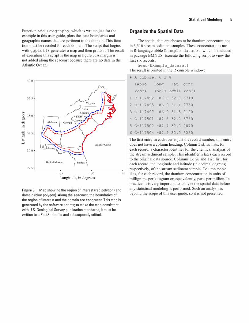
Function Add_Geography, which is written just for the example in this user guide, plots the state boundaries and geographic names that are pertinent to the domain. This func-tion must be recoded for each domain. The script that begins with ggplot() generates a map and then prints it. The result of executing this script is the map in figure 3. A margin is not added along the seacoast because there are no data in the Atlantic Ocean.

Figure 3. Map showing the region of interest (red polygon) and domain (blue polygon). Along the seacoast, the boundaries of the region of interest and the domain are congruent. This map is generated by the software scripts; to make the map consistent with U.S. Geological Survey publication standards, it must be written to a PostScript file and subsequently edited.

Organize the Spatial Data

The spatial data are chosen to be titanium concentrations in 3,316 stream sediment samples. These concentrations are in R-language tibble Example_dataset, which is included in package BMNUS. Execute the following script to view the first six records:

head(Example_dataset)The result is printed in the R console window:

# A tibble: 6 x 4

labno long lat conc

<chr> <dbl> <dbl> <dbl>

1 C-117492 -88.0 32.0 3710

2 C-117495 -86.9 31.4 2750

3 C-117497 -86.9 31.5 2120

4 C-117501 -87.8 32.0 3780

5 C-117502 -87.7 32.0 2870

6 C-117504 -87.9 32.0 3250

The first entry in each row is just the record number; this entry does not have a column heading. Column labno lists, for each record, a character identifier for the chemical analysis of the stream sediment sample. This identifier relates each record to the original data source. Columns long and lat list, for each record, the longitude and latitude (in decimal degrees), respectively, of the stream sediment sample. Column conc lists, for each record, the titanium concentration in units of milligrams per kilogram or, equivalently, parts per million. In practice, it is very important to analyze the spatial data before any statistical modeling is performed. Such an analysis is beyond the scope of this user guide, so it is not presented.

Alabama Georgia

SouthCarolina

NorthCarolina

Virginia

Florida

Atlantic Ocean

Gulf of Mexico

27.5

30.0

32.5

35.0

37.5

40.0

−85 −80 −75Longitude, in degrees

Latit

ude,

in d

egre

es


To map the locations of the titanium concentrations, execute this script:

ggplot() +


Add_Path(Example_domain, “blue”) +


Add_Points(Example_dataset) +


The resulting map is shown in figure 4. All sample locations are within the domain. In practice, the sample locations affect how the region of interest and the domain are delineated.

Figure 4. Map showing locations of the stream sediment samples (black dots). The red and blue polygons represent, respectively, the region of interest and the domain. Along the seacoast, the boundaries of the region of interest and the domain are congruent. This map is generated by the software scripts; to make the map consistent with U.S. Geological Survey publication standards, it must be written to a PostScript file and subsequently edited.

The data in Example_dataset are reorganized to facilitate processing. To this end, execute the following scripts:

Value <- scaledLogit(Example_dataset$conc, constSumValue = 1e6)

spatialData <-

sp::SpatialPointsDataFrame(data.frame(long = Example_dataset$long,

lat = Example_dataset$lat,

row.names = Example_dataset$labno),

data.frame(Value = Value,

IndValue = “no”,

me_sd = rep.int(me_sd, length(Value)),

row.names = Example_dataset$labno),

proj4string=sp::CRS(Example_CRS_arg_longlat),

match.ID=TRUE)

These measurements, which are transformed concentrations for this example, are stored in a SpatialPointsDataFrame, which is defined in the sp package and is designed specifically for spatial data. The first argument to SpatialPoints-DataFrame is an R-language dataframe that stores the longitudes and latitudes of the measurements. Note that the respective

Alabama Georgia

SouthCarolina

NorthCarolina

Virginia

Florida

Atlantic Ocean

Gulf of Mexico

27.5

30.0

32.5

35.0

37.5

40.0


Latit

ude,

in d

egre

es


column names must be long and lat. The second argument is an R-language dataframe that stores the measurements, the cen-sor indicators, and the standard deviations of the measurement errors. Note that the respective column names must be Value, IndValue, and me_sd. The censor indicators and standard deviations are described below. The third argument contains information about the datum that is used for the locations; this information is stored in character string Example_CRS_arg_longlat, which is included in the BMNUS package. The fourth argument tells the function to check whether the row names in the first and second arguments match.

Occasionally, some of the measurements are left or right censored. This information is important in the statistical model-ing and is stored in IndValue. The elements in IndValue are characters strings that have values left, right, or no. If an element is left, then the corresponding element in Value is left censored and is set to its censoring threshold. If an element is right, then the corresponding element in Value is right censored and is set to its censoring threshold. If an element is no, then the corresponding element in Value is not censored. (For the titanium concentrations, no measurements are censored, so all elements in IndValue are no.) It is acceptable to have multiple censoring thresholds.

The standard deviation of the measurement error is specified for each measurement. This specification is redundant for the example presented in this user guide because the standard deviation is the same for all measurements. However, the standard deviation changes in some cases; for example, the measurements could comprise two or more datasets with different measure-ment errors. In such cases, specification for each measurement is necessary.

Generate the Basis Functions

The individual basis function is a local bi-square function (Cressie and Johannesson, 2008), which is nonzero in a circu-lar region around its center and is zero everywhere else. This individual basis function is placed at regularly spaced intervals throughout the domain. Thus, a key parameter is the spacing between the individual basis functions; this spacing is unknown at this stage in the modeling. Consequently, the data are modeled using a wide range of different spacings, and the modeling results for a specific spacing are selected according to a quantitative measure. This procedure is described in the next section. The cur-rent modeling step is to select a suitable set of spacings and then to generate the basis functions for those spacings.

A way to select a suitable set is to plot the transformed concentrations along several different transects through the domain. To this end, execute the following scripts to generate and display one transect:

maxOffset <- 10

end_points1 <- data.frame(long = c(-83.48355, -81.21104),

lat = c(33.30348, 29.69067))

oViewTransect1 <- ViewTransect(spatialData, maxOffset, end_points1,

Example_CRS_arg_utm)

plotSampleLocations(oViewTransect1) +

Add_Geography() +

Add_Path(Example_domain, color = “blue”) +

Refine_Map(“lambert”, 25, 40,

latLimits = c(29, 34),

longLimits = c(-85.5, -80))

plot(oViewTransect1, “Ilr-transformed\nconcentration”, span = 0.5, se = FALSE)

The first script specifies the maximum offset between the transect and a field sample; this specification effectively defines which field samples are included in the transect. The unit for offset is a kilometer. The second script specifies the end points of the transect, using longitude and latitude. The third script calls a constructor for class ViewTransect, which is used to gener-ate the transect from the spatial data. The fourth script plots the transect and the field samples that are included in the transect (fig. 5). The fifth script plots the transformed concentrations as a function of distance along the transect (fig. 6).


Figure 5. Graph showing the transect (red line), the field samples associated with the transect (black dots), and a portion of the domain boundary (blue lines). This graph is generated by the software scripts; to make it consistent with U.S. Geological Survey publication standards, it must be written to a PostScript file and subsequently edited.

Figure 6. Graph showing the transformed concentrations (black dots) along the transect (fig. 5), and a smooth curve (red line) that is fit to the transformed concentrations. This graph is generated by the software scripts; to make it consistent with U.S. Geological Survey publication standards, it must be written to a PostScript file and subsequently edited.

29

30

31

32

33

34


Latit

ude,

in d

egre

es

−5.0

−4.5

−4.0

−3.5

−3.0

0 100 200 300 400Distance, in kilometers

Ilr−transfo

rmed

conc

entra

tion


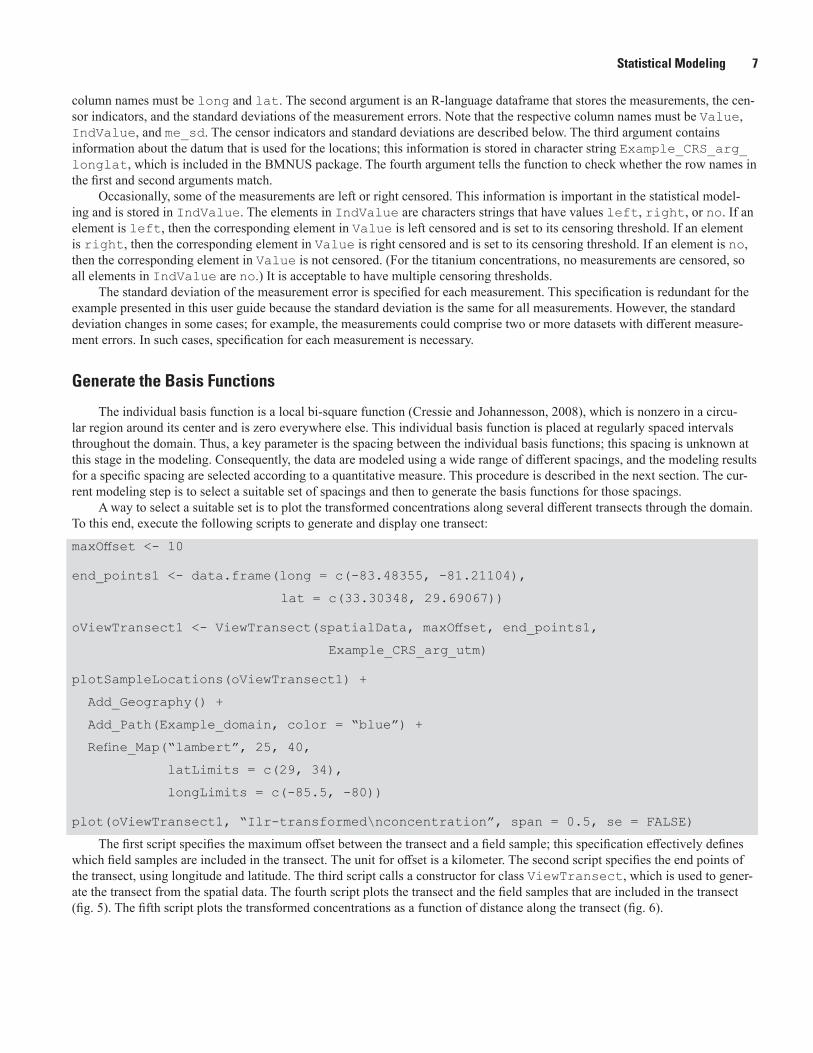
The transformed concentrations are highly variable (fig 6), making it difficult to discern the length of the smallest feature that could be resolved. A reasonable guess of this length might be 50 km. This guess applies also to three other transects that are not shown here, but their scripts are presented in file ScriptsInUsersGuide.R.

To resolve a feature that is 50 km across, the spacing between the basis function centers must be 50 km or less. Because this spacing is just a guess, basis functions are generated for spacings ranging from 20 to 100 km, using the following scripts:

spacings <- c(“020”, “025”, “030”, “035”, “040”,

“045”, “050”, “055”, “060”,

“070”, “080”, “090”, “100”)

oBasisFunctions <- BasisFunctions(spacings,

Example_domain,

spatialData,

Example_CRS_arg_utm,

seed = 777)

summary(oBasisFunctions)

plot(oBasisFunctions, 30) +




The first script specifies, as character strings, the spacings between the basis function centers. The unit for the spacing is kilome-ters. The second script calls a constructor for the class that calculates the basis functions. The basis functions for each spacing are written to a file in directory BasisFunctions, which is created by the constructor. The third script prints, for each spacing, information about the matrix that stores the values of the basis functions at the locations of the field samples. The fourth script plots locations of the basis function centers for a spacing of 30 km (fig. 7). Notice that the centers extend slightly beyond the boundary of the domain; this feature improves the accuracy of the modeling within the domain. However, along a small part of the seacoast of North Carolina, the centers do not extend beyond the boundary because there are too few field samples to do so (fig. 4). To plot the locations of the basis function centers for any other spacing, only the second argument to function plot is changed; scripts for spacings of 20, 50, 70, and 100 km are presented in file ScriptsInUsersGuide.R.

Figure 7. Map showing locations (black dots) of the centers of the basis functions for a spacing of 30 kilometers. The red and blue polygons represent, respectively, the region of interest and the domain. Along the seacoast, the boundaries of the region of interest and the domain are congruent. This map is generated by the software scripts; to make the map consistent with U.S. Geological Survey publication standards, it must be written to a PostScript file and subsequently edited.

Alabama Georgia

SouthCarolina

NorthCarolina

Virginia

Florida

Atlantic Ocean

Gulf of Mexico

27.5

30.0

32.5

35.0

37.5

40.0


Latit

ude,

in d

egre

es

Spacing: 30 kilometers


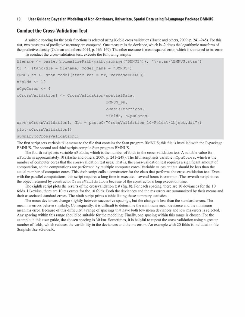
Conduct the Cross-Validation Test

A suitable spacing for the basis functions is selected using K-fold cross validation (Hastie and others, 2009, p. 241–245). For this test, two measures of predictive accuracy are computed. One measure is the deviance, which is -2 times the logarithmic transform of the predictive density (Gelman and others, 2014, p. 166–169). The other measure is mean squared error, which is shortened to ms error.

To conduct the cross-validation test, execute the following scripts:

filename <- paste0(normalizePath(path.package(“BMNUS”)), “\\stan\\BMNUS.stan”)

tr <- stanc(file = filename, model_name = “BMNUS”)

BMNUS_sm <- stan_model(stanc_ret = tr, verbose=FALSE)

nFolds <- 10

nCpuCores <- 4

oCrossValidation1 <- CrossValidation(spatialData,

BMNUS_sm,

oBasisFunctions,

nFolds, nCpuCores)

save(oCrossValidation1, file = paste0(“CrossValidation_10-Folds\\Object.dat”))

plot(oCrossValidation1)

summary(oCrossValidation1)

The first script sets variable filename to the file that contains the Stan program BMNUS; this file is installed with the R-package BMNUS. The second and third scripts compile Stan program BMNUS.

The fourth script sets variable nFolds, which is the number of folds in the cross-validation test. A suitable value for nFolds is approximately 10 (Hastie and others, 2009, p. 241–249). The fifth script sets variable nCpuCores, which is the number of computer cores that the cross-validation test uses. That is, the cross-validation test requires a significant amount of computation, so the computations are performed by multiple computer cores. Variable nCpuCores should be less than the actual number of computer cores. This sixth script calls a constructor for the class that performs the cross-validation test. Even with the parallel computations, this script requires a long time to execute—several hours is common. The seventh script stores the object returned by constructor CrossValidation because of the constructor’s long execution time.

The eighth script plots the results of the crossvalidation test (fig. 8). For each spacing, there are 10 deviances for the 10 folds. Likewise, there are 10 ms errors for the 10 folds. Both the deviances and the ms errors are summarized by their means and their associated standard errors. The ninth script prints a table listing these summary statistics.

The mean deviances change slightly between successive spacings, but the change is less than the standard errors. The mean ms errors behave similarly. Consequently, it is difficult to determine the minimum mean deviance and the minimum mean ms error. Because of this difficulty, a range of spacings that have both low mean deviances and low ms errors is selected. Any spacing within this range should be suitable for the modeling. Finally, one spacing within this range is chosen. For the example in this user guide, the chosen spacing is 30 km. Sometimes, it is helpful to repeat the cross validation using a greater number of folds, which reduces the variability in the deviances and the ms errors. An example with 20 folds is included in file ScriptsInUsersGuide.R.


Figure 8. Graphs showing results of the cross-validation test with 10 folds. A, Test results for the deviance. A gray dot represents a deviance. (A small amount of random noise is added to the horizontal coordinate to reduce the number of symbols plotting atop one another.) A red dot represents the mean of the 10 deviances at a specified spacing; each vertical red line associated with a red dot represent one standard error for the mean. B, Test results for the mean squared error. The definitions of the graph elements are analogous to those in A. This graph is generated by the software scripts; to make it consistent with U.S. Geological Survey publication standards, it must be written to a PostScript file and subsequently edited.

Sample the Posterior Probability Density Function

To sample the posterior probability density function, execute the following scripts:

load(“BasisFunctions\\Spacing_030.dat”)csrBasisFuncs <- as(basis_functions$basisFuncs, “RsparseMatrix”)carQuantities <- SparseCarQuantities(basis_functions)stanData <- list( N = nrow(spatialData@data), M = ncol(csrBasisFuncs), UU = csrBasisFuncs@p + 1, VV = csrBasisFuncs@j + 1, WW = csrBasisFuncs@x, nNeighborPairs = carQuantities$nNeighborPairs, W_sparse = carQuantities$W_sparse, D_sparse = carQuantities$D_sparse, lambda = carQuantities$lambda, X = spatialData@data$Value, me_sd = spatialData@data$me_sd, areLeftCensored = as.integer( spatialData@data$IndValue == “left”), betaPar = c(2.5, 1.2), gammaPar = c(2, 0.3), cauchyPar = 3)gen_init <- function(){ phi1 <- rnorm(stanData$M, mean = 0.0, sd = 1e-6) phi2 <- rnorm(stanData$M, mean = 0.0, sd = 1e-6) return(list(phi1 = phi1, phi2 = phi2))}nChains <- 3

100

150

200

20 25 30 35 40 45 50 55 60 70 80 90 100Distance between basis function centers , in kilometers

Dev

ianc

e

A.

0.08

0.10

0.12

0.14

20 25 30 35 40 45 50 55 60 70 80 90 100Distance between basis function centers , in kilometers

Mea

n sq

uare

d er

ror B.


if(nChains < parallel::detectCores()){ oldPar <- options(mc.cores = nChains) } else{ oldPar <- options(mc.cores = parallel::detectCores()-1) }rawSamples <- sampling(BMNUS_sm, data = stanData, chains = nChains, iter = 2000, warmup = 500, refresh = 100, seed = 7, init = gen_init, pars=c(“phi1”, “tau1”, “alpha1”, “phi2”, “tau2”, “alpha2”, “rho”, “Y_mean”, “Y_sd”))

options(oldPar)

The first script loads, into computer memory, the basis functions for which the spacing is 30 km. The second function converts the basis-function matrix from dictionary-of-keys format to compressed, sparse, row-oriented format, which is needed by the BMNUS program. The third script calculates quantities (namely, a scalar, two vectors, and a matrix) that are needed to implement the sparse, conditional auto-regressive model. The fourth script prepares the data container for the BMNUS program. The vari-ables in this list are completely described in file BMNUS.stan, which is in the BMNUS package, so the description is not repeated here. The fifth script is a function that is used to initialize vectors phi1 and phi2 in the Stan program BMNUS—this initializa-tion facilitates sampling of the posterior probability density function. The sixth script sets the number of chains in the sampler. The seventh script, which comprises the block-if expression, sets the number of cores for the sampling of the posterior probability density function—it is very important that the number of cores for the sampling be less than the actual number of cores.

Finally, the eighth script performs the sampling. The posterior probability density function is sampled three times, yield-ing three chains. Each chain consists of 2,000 samples of which the first 500 samples are warmup. Progress on the sampling is printed every 100 samples. The seed for random number generation is set to a specific value (namely, 7) so that the results in this user guide can be reproduced exactly. (However, the seed should not be set for most applications.) The nine parameters for which samples are returned are listed in function argument pars. Parameter phi1 comprises the basis function weights associ-ated with the process mean; parameter phi2 comprises the weights associated with the process standard deviation. Parameters Y_mean and Y_sd are, respectively, the mean of the process model and the standard deviation of the process model at the loca-tions of the field samples. Parameter rho is the average standard deviation throughout the domain. The remaining four param-eters are related to the conditional autoregressive model and are described in Ellefsen and Van Gosen (2019). The ninth script sets the number of cores for the sampling to its original value.

The sampling requires a long time, so it is prudent to save the results; to this end, execute the following scripts:

if(!dir.exists(“SamplingResults”)){

dir.create(“SamplingResults”)

}

save(stanData, rawSamples, file = “SamplingResults\\RawSamples.dat”)

The scripts associated with the if-statement check whether directory SamplingResults exists. If not, the directory is created. The last script writes the sampling results in a file.


Check Convergence

A summary of selected parameters in the posterior probability density function is written to a file with the following scripts:

filename <- paste(“SamplingResults\\Summary.txt”, sep = “”)

oldPars <- options(width = 140, max.print = 100000)

sink(filename)

print(rawSamples, digits = 3,

pars = c(“tau1”, “alpha1”, “tau2”, “alpha2”, “rho”))

sink()

options(width = oldPars$width, max.print = oldPars$max.print)

These scripts involve common R functions, so they are not described here. The summary is as follows:

Inference for Stan model: BMNUS.

3 chains, each with iter=2000; warmup=500; thin=1;

post-warmup draws per chain=1500, total post-warmup draws=4500.

mean se_mean sd 2.5% 25% 50% 75% 97.5% n_eff Rhat

tau1 19.945 0.137 3.090 14.557 17.745 19.715 21.944 26.616 507 1.011

alpha1 0.971 0.000 0.017 0.932 0.962 0.974 0.984 0.995 2270 1.001

tau2 6.627 0.112 1.743 3.789 5.386 6.425 7.670 10.607 242 1.011

alpha2 0.827 0.006 0.101 0.573 0.774 0.847 0.902 0.963 327 1.008

rho 0.278 0.001 0.016 0.249 0.268 0.277 0.288 0.313 685 1.004

Samples were drawn using NUTS(diag_e) at Tue Sep 24 15:40:12 2019.

For each parameter, n_eff is a crude measure of effective sample size,

and Rhat is the potential scale reduction factor on split chains (at

convergence, Rhat=1).

Regarding convergence, there are two key statistics. The first is the effective number of independent simulation draws (n_eff). It should be at least 10 percent of the total number of samples, and larger values are even better. Because there are 3 chains of 1,500 samples (after warmup), the total number of samples is 4,500; thus, the lower threshold for n_eff is 450. This criterion is met for all parameters except tau2 and alpha2. In our experience, it is common that the parameters in this sum-mary have relatively low values of n_eff. The reason is that these parameters are deep in the hierarchical model, making them difficult to sample. Because these parameters are not used for inference, the low values of n_eff are inconsequential. Additional information on the effective number of independent simulation draws is in Gelman and others (2014, p. 286–288).

The other statistic that assesses convergence is the potential scale-reduction factor (Rhat). This factor indicates how much the scale of a parameter could be reduced if the number of samples of the posterior probability density function were increased to infinity (Gelman and others, 2014, p. 284–285); that is, values near 1 indicate that the sampling has converged. This factor should be between 0.95 and 1.05—values outside this range indicate possible problems with convergence. All parameters in this summary meet this criterion. In our experience, the other parameters—phi1, phi2, Y_mean, and Y_sd—always meet this criterion.


The best way to assess convergence is to use Rpackage shinystan. To this end, execute these scripts:

library(shinystan)

launch_shinystan(rawSamples)

A description of shinystan is beyond the scope of this user guide but is available in the help information that accompanies shinystan.

Check the Statistical Model

The first check of the statistical model involves analyzing the fit between the model and the data along one or more tran-sects within the domain. In this user guide, one transect is analyzed. Execute the following scripts:

end_points <- data.frame(long = c(-83.48355, -81.21104),

lat = c(33.30348, 29.69067))

maxOffset <- 10

oCheckTransect <- CheckTransect(spatialData, maxOffset, end_points,

Example_CRS_arg_utm)

plotSampleLocations(oCheckTransect) +

Add_Geography() +

Add_Path(Example_domain, color = “blue”) +

Refine_Map(“lambert”, 25, 40,

latLimits = c(29, 34),

longLimits = c(-85.5, -80))

The first script sets the locations of the transect ends. The second script sets the maximum offset between the transect and a field sample; the maximum offset effectively specifies which field samples are included in the transect. The unit for the maximum offset is a kilometer. The third script calls a constructor for the class that generates the transect. The fourth script plots the tran-sect, the field points associated with it, and some geographical details (fig. 9). This plot is used to check both the transect and the maximum offset: the transect should be within the domain, and there should be enough field samples to analyze the fit between the model and the data. A suitable number might be between 20 and 100.

Figure 9. Map showing the transect (red line), field samples associated with the transect (black dots), and a portion of the domain boundary (blue lines). This map is generated by the software scripts; to make the map consistent with U.S. Geological Survey publication standards, it must be written to a PostScript file and subsequently edited.

29

30

31

32

33

34


Latit

ude,

in d

egre

es


Execute the following script to analyze the fit between the model and the data:

plot(oCheckTransect, rawSamples, “Ilr-transformed\nconcentration”)

This script generates four plots, all of which are functions of the distance along the transect (fig. 10). These plots are discussed in appendix 1 of Ellefsen and Van Gosen (2019).

Figure 10. Graphs used to check, along a transect, the fit of the model to the data. A, Measured values of the field samples. B, Distributions of the process mean at the locations of the field samples. C, Distributions of the process standard deviation at the locations of the field samples. D, Distributions of the predicted measurements at the locations of the field samples and the measured values of the field samples (red dots). In the plot symbol representing a distribution, the bottom and the top of the vertical line represent its 0.025 and 0.975 quantiles, and the black dot represents its 0.50 quantile. These graphs are generated by the software scripts; to make them consistent with U.S. Geological Survey publication standards, they must be written to a PostScript file and subsequently edited.

−5.0−4.5−4.0−3.5−3.0


Ilr−t

rans

form

edco

ncen

tratio

n

A. Data

−5.0−4.5−4.0−3.5−3.0


Ilr−t

rans

form

edco

ncen

tratio

n

B. Process Mean

0.10.20.30.40.50.60.7


Ilr−t

rans

form

edco

ncen

tratio

n

C. Process Standard Deviation

−5.0−4.5−4.0−3.5−3.0


Ilr−t

rans

form

edco

ncen

tratio

n

D. Predicted Measurements and Data


The second check of the statistical model involves comparing the measured values to simulated values, which are generated with model. This check is most easily performed using data along a transect, and the transect that is defined in the beginning of the section is used. Execute the following script:

plotSimulatedTransects(oCheckTransect, rawSamples, “Ilr-transformed\nconcentration”)

This script generates 8 plots—1 plot for the measured values, and 7 plots for 7 sets of simulated values (fig. 11). These plots are discussed in appendix 1 of Ellefsen and Van Gosen (2019).

Figure 11. Graphs used to compare, A, the measured values and, B–H, simulated values. These graphs pertain to the transect in figure 9. These graphs are generated by the software scripts; to make them consistent with U.S. Geological Survey publication standards, they must be written to a PostScript file and subsequently edited.

−5.0−4.5−4.0−3.5−3.0


Ilr−t

rans

form

edco

ncen

tratio

n

A. Measured

−5.0−4.5−4.0−3.5−3.0


Ilr−t

rans

form

edco

ncen

tratio

n

B. Simulated

−5.0−4.5−4.0−3.5−3.0


Ilr−t

rans

form

edco

ncen

tratio

n

C. Simulated

−5.0−4.5−4.0−3.5−3.0


Ilr−t

rans

form

edco

ncen

tratio

n

D. Simulated

−5.0−4.5−4.0−3.5−3.0


Ilr−t

rans

form

edco

ncen

tratio

n

E. Simulated

−5.0−4.5−4.0−3.5−3.0


Ilr−t

rans

form

edco

ncen

tratio

nF. Simulated

−5.0−4.5−4.0−3.5−3.0


Ilr−t

rans

form

edco

ncen

tratio

n

G. Simulated

−5.0−4.5−4.0−3.5−3.0


Ilr−t

rans

form

edco

ncen

tratio

n

H. Simulated


The third check of the statistical model involves analyzing the statistical properties of the standardized residuals. To this end, execute the following scripts:

oCheckResiduals <- CheckResiduals(stanData, rawSamples)

plot(oCheckResiduals, spatialData, Example_CRS_arg_utm,

variogram_breaks = seq(from = 0, to = 150, length.out = 16))

summary(oCheckResiduals)

The first script calls the class constructor for the standardized residuals, which calculates the standardized residuals and various summary statistics. The second script plots three graphs that help analyze the standardized residuals (fig. 12). The third script prints the following table that summarizes the standardized residuals:

#########################################################################

Summary of the standardized residuals

Number = 3316

Range: -4.25513 4.12386

Mean = -0.0036397

Standard deviation = 0.940554

Skewness = -0.342551

Median = 0.0633641

IQR = 1.20675

########################################################################

Both the graphs (fig. 12) and the table are discussed in appendix 1 of Ellefsen and Van Gosen (2019).

Figure 12. Graphs used to analyze the statistical properties of the standardized residuals. A, Histogram. B, Quantile-quantile plot. The green line represents equality between the standardized residuals and the corresponding quantiles of the standard normal distribution. C, Semi-variogram. The green line represents the variance of the standardized residuals. These graphs are generated by the software scripts; to make them consistent with U.S. Geological Survey publication standards, they must be written to a PostScript file and subsequently edited.

0.0

0.1

0.2

0.3

0.4

−2.5 0.0 2.5Standardized residual

Den

sity

A.

−2.5

0.0

2.5

−2.5 0.0 2.5Quantile of standardnormal distribution

Qua

ntile

of

stan

dard

ized

resi

dual

s

B.

0.00

0.25

0.50

0.75

0 50 100 150Distance, in kilometers

Sem

ivar

iogr

am

C.


The fourth check of the statistical model involves mapping the arithmetic sign of the standardized residuals. The map (fig. 13) is generated with the following script: plotResidualMap(oCheckResiduals, spatialData, shape = 16, size = 0.9) +


Refine_Map(“lambert”, 25, 40, latLimits = c(28, 39.5)) +

Refine_Legend(c(0.02,0.99), c(0,1)) +

guides(colour = guide_legend(override.aes = list(size = 3))) +

theme(legend.key = element_rect(fill = “gray90”))

This map is discussed in appendix 1 of Ellefsen and Van Gosen (2019).

Figure 13. Map showing the arithmetic sign of the standardized residuals. This map is generated by the software scripts; to make the map consistent with U.S. Geological Survey publication standards, it must be written to a PostScript file and subsequently edited.

Map the Predicted QuantitiesThe quantities that may be predicted are the process mean, the process standard deviation, a specified quantile, and a

specified exceedance probability. To map these quantities, they are predicted on a grid of uniformly spaced points that cover the domain. To perform the prediction, execute the following scripts:threshold <- scaledLogit(8000, constSumValue = 1e6)

oPredictions <- Prediction(Example_domain,

spatialData,

Example_CRS_arg_utm,

basis_functions,

rawSamples,

threshold)

plotPredictionLocations(oPredictions, fraction = 1/3) +




plotPalette <- colorRampPalette(c(“blue”, “green”,

“yellow”, “orange”, “red”, “black”))(12)

Alabama Georgia

SouthCarolina

NorthCarolina

Virginia

Florida

Atlantic Ocean

Gulf of Mexico

27.5

30.0

32.5

35.0

37.5

40.0


Latit

ude,

in d

egre

es

Arithmetic sign

Negative

Positive


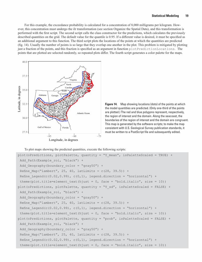
For this example, the exceedance probability is calculated for a concentration of 8,000 milligrams per kilogram. How-ever, this concentration must undergo the ilr transformation (see section Organize the Spatial Data), and this transformation is performed with the first script. The second script calls the class constructor for the predictions, which calculates the previously described quantities on the grid. The default value for the quantile is 0.95. If a different value is desired, it must be specified as an additional argument to this function. The third script plots the locations of the points at which the quantities are predicted (fig. 14). Usually the number of points is so large that they overlap one another in the plot. This problem is mitigated by plotting just a fraction of the points, and this fraction is specified as an argument in function plotPredictionLocations. The points that are plotted are selected randomly, so repeated plots differ. The fourth script generates a color palette for the maps.

Figure 14. Map showing locations (dots) of the points at which the model quantities are predicted. (Only one-third of the points are plotted.) The red and blue polygons represent, respectively, the region of interest and the domain. Along the seacoast, the boundaries of the region of interest and the domain are congruent. This map is generated by the software scripts; to make the map consistent with U.S. Geological Survey publication standards, it must be written to a PostScript file and subsequently edited.

To plot maps showing the predicted quantities, execute the following scripts:

plot(oPredictions, plotPalette, quantity = “Y_mean”, isPaletteScaled = TRUE) +

Add_Path(Example_roi, “black”) +



Refine_Legend(c(0.02,0.99), c(0,1), legend.direction = “horizontal”) +

theme(plot.title=element_text(hjust = 0, face = “bold.italic”, size = 10))

plot(oPredictions, plotPalette, quantity = “Y_sd”, isPaletteScaled = FALSE) +






plot(oPredictions, plotPalette, quantity = “prob”, isPaletteScaled = FALSE) +






Alabama Georgia

SouthCarolina

NorthCarolina

Virginia

Florida

Atlantic Ocean

Gulf of Mexico

27.5

30.0

32.5

35.0

37.5

40.0


Latit

ude,

in d

egre

es


plot(oPredictions, plotPalette, quantity = “quantile”, isPaletteScaled = TRUE) +






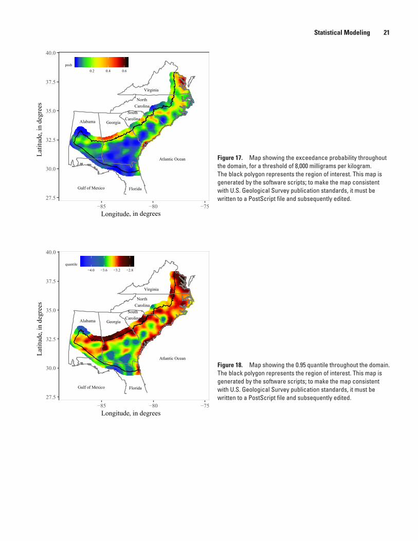
These four scripts plot, respectively, maps of the process mean (fig. 15), the process standard deviation (fig. 16), the exceedance probability (fig. 17), and the 0.95 quantile (fig. 18).

Figure 16. Map showing the process standard deviation throughout the domain. The black polygon represents the region of interest. This map is generated by the software scripts; to make the map consistent with U.S. Geological Survey publication standards, it must be written to a PostScript file and subsequently edited.

Figure 15. Map showing the process mean throughout the domain. The black polygon represents the region of interest. This map is generated by the software scripts; to make the map consistent with U.S. Geological Survey publication standards, it must be written to a PostScript file and subsequently edited.

Alabama Georgia

SouthCarolina

NorthCarolina

Virginia

Florida

Atlantic Ocean

Gulf of Mexico

27.5

30.0

32.5

35.0

37.5

40.0


Latit

ude,

in d

egre

es

−4.5 −4.0 −3.5Y_mean

Alabama Georgia

SouthCarolina

NorthCarolina

Virginia

Florida

Atlantic Ocean

Gulf of Mexico

27.5

30.0

32.5

35.0

37.5

40.0


Latit

ude,

in d

egre

es

0.2 0.4 0.6 0.8Y_sd


Figure 17. Map showing the exceedance probability throughout the domain, for a threshold of 8,000 milligrams per kilogram. The black polygon represents the region of interest. This map is generated by the software scripts; to make the map consistent with U.S. Geological Survey publication standards, it must be written to a PostScript file and subsequently edited.

Figure 18. Map showing the 0.95 quantile throughout the domain. The black polygon represents the region of interest. This map is generated by the software scripts; to make the map consistent with U.S. Geological Survey publication standards, it must be written to a PostScript file and subsequently edited.

Alabama Georgia

SouthCarolina

NorthCarolina

Virginia

Florida

Atlantic Ocean

Gulf of Mexico

27.5

30.0

32.5

35.0

37.5

40.0


Latit

ude,

in d

egre

es

0.2 0.4 0.6prob

Alabama Georgia

SouthCarolina

NorthCarolina

Virginia

Florida

Atlantic Ocean

Gulf of Mexico

27.5

30.0

32.5

35.0

37.5

40.0


Latit

ude,

in d

egre

es

−4.0 −3.6 −3.2 −2.8quantile


For the example in this user guide, the measurements are the ilr transform of the titanium concentrations (see section Organize the Spatial Data). Consequently, maps for the process mean (fig. 15), the process standard deviation (fig. 16), and the 0.95 quantile (fig. 18) relate to the ilr transform of the titanium concentrations. To make the maps of the process mean and the 0.95 quantile easily interpretable, the labels for the color bar should be re-expressed as titanium concentration with units of milligrams per kilogram. For example, the labels for the process mean are −4.5, −4.0, and −3.5. These labels are transformed to their equivalent labels in units of milligrams per kilogram with the following script:

invScaledLogit(c(-4.5, -4.0, -3.5), constSumValue = 1e6)

The equivalent labels are 1720, 3480, and 7040 milligrams per kilogram. That is, the map should be written to a PostScript file, and the labels on the color bar should be replaced by the equivalent labels. No transformation exists for the process standard deviation; this issue is discussed further in Ellefsen and Van Gosen (2019).

Data, Software, and ReproducibilityThe data are in Rpackage BMNUS, which accompanies this user guide. The software scripts in this user guide are in the

compressed file ReportScripts.zip, which accompanies the user guide. You are encouraged to execute the software scripts to repro-duce the results in this report and thereby check the calculations and figures. Please report any errors to the authors.

AcknowledgmentsThis work was funded by the project Heavy-Mineral Sand Resources in the Southeastern U.S.within the Mineral Resources

Program of the U.S. Geological Survey. K.E. Livo and W.H. Asquith reviewed the manuscript, and their suggestions improved the manuscript.

References Cited

Carpenter, B., Gelman, A., Hoffman, M.D., Lee, D., Goodrich, B., Betancourt, M., Brubaker, M., Guo, J., Li, P., and Riddell, A., 2017, Stan—A probabilistic programming language: Journal of Statistical Software, v. 76, no. 1. [Also available at https://doi.org/10.18637/jss.v076.i01.]

Cressie, N., and Johannesson, G., 2008, Fixed rank kriging for very large spatial data sets: Journal of the Royal Statistical Society, Series B, Statistical Methodology, v. 70, no. 1, p. 209–226. [Also available at https://doi.org/10.1111/j.1467-9868.2007.00633.x.]

Ellefsen, K.J., and Van Gosen, B.S., 2020, Bayesian modeling of non-stationary, univariate, spatial data for the Earth sci-ences: U.S. Geological Survey Techniques and Methods, book 7, chap. C24, 20 p. [Also available at https://doi.org/ 10.3133/tm7C24.]

Hastie, T., Tibshirani, R., and Friedman, J., 2009, The elements of statistical learning—Data mining, inference, and prediction, 2nd ed.: New York, Springer Science+Business Media, 745 p.

Gelman, A., Carlin, J.B., Stern, H.S., Dunson, D.B., Vehtari, A., and Rubin, D.B., 2014, Bayesian data analysis (3d ed.): Boca Raton, CRC Press, 661 p.

Pawlowsky-Glahn, V., Egozcue, J.J., and Tolosana-Delgado, R., 2015, Modeling and analysis of compositional data: Chichester, England, John Wiley and Sons, Ltd., 247 p.

R Development Core Team, 2019, R—A language and environment for statistical computing: R Foundation for Statistical Com-puting, https://www.R-project.org/.

Reimann, C., Filmoser, P., Garrett, R. G., and Dutter, R., 2008, Statistical data analysis explained—Applied environmental sta-tistics with R: Chichester, West Sussex, John Wiley and Sons, Ltd., 343 p.

https://doi.org/10.18637/jss.v076.i01

https://doi.org/10.18637/jss.v076.i01

https://doi.org/10.1111/j.1467-9868.2007.00633.x

https://doi.org/10.1111/j.1467-9868.2007.00633.x

https://doi.org/%2010.3133/tm7C24

https://doi.org/%2010.3133/tm7C24

https://www.R-project.org/

Appendix 1 23

Appendix 1. Estimate the Standard Deviation of the Measurement Error using Paired Measurements

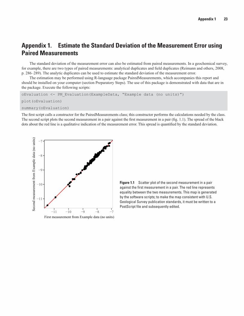
The standard deviation of the measurement error can also be estimated from paired measurements. In a geochemical survey, for example, there are two types of paired measurements: analytical duplicates and field duplicates (Reimann and others, 2008, p. 286–289). The analytic duplicates can be used to estimate the standard deviation of the measurement error.

The estimation may be performed using R-language package PairedMeasurements, which accompanies this report and should be installed on your computer (section Preparatory Steps). The use of this package is demonstrated with data that are in the package. Execute the following scripts:

oEvaluation <- PM_Evaluation(ExampleData, “Example data (no units)”)

plot(oEvaluation)

summary(oEvaluation)

The first script calls a constructor for the PairedMeasurements class; this constructor performs the calculations needed by the class. The second script plots the second measurement in a pair against the first measurement in a pair (fig. 1.1). The spread of the black dots about the red line is a qualitative indication of the measurement error. This spread is quantified by the standard deviation.

Figure 1.1 Scatter plot of the second measurement in a pair against the first measurement in a pair. The red line represents equality between the two measurements. This map is generated by the software scripts; to make the map consistent with U.S. Geological Survey publication standards, it must be written to a PostScript file and subsequently edited.

−11

−10

−9

−8

−7

−11 −10 −9 −8 −7First measurement from Example data (no units)

Seco

nd m

easu

rem

ent f

rom

Exa

mpl

e da

ta (n

o un

its)


The third script prints a table containing summary statistics for the pair measurements:

###############################################################

Summary

Number of paired measurements: 176

Range: -11.4631 -7.12777

Standard deviation of the paired measurements: 0.0398779

###############################################################

The standard deviation of the paired measurements is the standard deviation of the measurement error.

Appendix 2 25

Appendix 2. Reading and Writing Data for GIS ProgramsSome researchers will want to use geographic information system software with the BMNUS package. To facilitate such

use, the package includes four functions that read and write shapefiles, which are a standard geographic information system format to store data. Function read_polygon_shapefile is used to read a polygon that represents either the domain or the region of interest. Function read_point_shapefile is used to read the measurements, their censor indicators, and their locations. Function write_point_shapefile is used to write the predictions (namely, the process mean, the process standard deviation, the exceedance probability, and the quantile) and their locations. Function write_rasterfiles is used to write the predictions as raster files, for which the format is the GeoTiff metadata standard. Complete documentation for these functions is included in the package.


Appendix 3. Cross validation using a validation datasetIf there is both a training dataset and a validation dataset, then the cross-validation test is conducted with class

SimpleCrossValidation. To explain how this class is used, assume that the training dataset is stored in a SpatialPointsDataFrame that is called training_spatialData. Similarly, the validation dataset is stored in a SpatialPointsDataFrame that is called validation_spatialData. The format of these two SpatialPointsDataFrames is identical to that of spatialData, which is described in section Organize the Spatial Data.

To conduct the cross-validation test, execute the following scripts:

filename <- paste0(normalizePath(path.package(“BMNUS”)), “\\stan\\BMNUS.stan”)

tr <- stanc(file = filename, model_name = “BMNUS”)

BMNUS_sm <- stan_model(stanc_ret = tr, verbose=FALSE)

nCpuCores <- 4

oSimpleCrossValidation <- SimpleCrossValidation(training_spatialData,

validation_spatialData,

me_sd, BMNUS_sm,

oBasisFunctions,

nCpuCores)

save(oSimpleCrossValidation, file = “SimpleCrossValidation.dat”)

plot(oSimpleCrossValidation)

summary(oSimpleCrossValidation)

The first fours scripts are described in section Conduct the Cross-Validation Test. The fifth script calls a constructor for the class that performs the cross-validation test. The first two arguments to this constructor are the training and validation datasets. Even with the parallel computations, this script requires a long time to execute. The sixth script stores the object returned by construc-tor SimpleCrossValidation because of the constructor’s long execution time. The seventh script plots the results of the crossvalidation test. For each spacing, there is one deviance, and there is one ms error. The eighth script prints a table listing these measures of prediction accuracy.

Appendix 4 27

Appendix 4. Troubleshooting TipsWhen library rstan is installed, the installation program writes a file that contains various compiler options that are needed

when the Stan program BMNUS is compiled. These compiler options are appropriate for many computer processors but not all. For example, when these compiler options are used on author Ellefsen’s computer, Stan program BMNUS fails to execute properly: Function CrossValidation (see section Conduct the Cross-Validation Test), which uses Stan program BMNUS, gener-ates the following error message:

Error in unserialize(node$con) : error reading from connection.

If you see such an error message, then the compiler options on your computer must be changed. To this end, locate file Make-vars.win. (On author Ellefsen’s computer, this file is in directory C:\Users\ellefsen\Documents\.R\. Replace the contents of this file with the following:

CXX14 = g++ -std=c++1y

CXX14FLAGS=-O3 -Wno-unused-variable -Wno-unused-function

CXX11FLAGS=-O3

Finally, recompile the Stan program BMNUS (see section Conduct the Cross-Validation Test).

Ellefsen and others—U

ser Guide to B

ayesian Modeling of N

on-Stationary, Univariate, Spatial D

ata Using R-Language Package B

MN

US—

TM 7–C20

ISSN 2328-7055 (online)https://doi.org/10.3133/tm7C20

https://doi.org/10.3133/tm7C20