user’s guide for smokeview version 4 - a tool for ...€¦ · nist special publication 1017...
TRANSCRIPT
NIST Special Publication 1017
User’s Guide for Smokeview Version 4- A Tool for Visualizing Fire Dynamics
Simulation Data
Glenn P. ForneyKevin B. McGrattan
NIST Special Publication 1017
User’s Guide for Smokeview Version 4- A Tool for Visualizing Fire Dynamics
Simulation Data
Glenn P. ForneyKevin B. McGrattan
Fire Research DivisionBuilding and Fire Research Laboratory
August 2004
UN
ITE
DSTATES OF AM
ER
ICA
DE
PARTMENT OF COMMERC
E
U.S. Department of CommerceDonald L. Evans, Secretary
Technology AdministrationPhillip J. Bond, Under Secretary for Technology
National Institute of Standards and TechnologyArden L. Bement, Jr., Director
Certain commercial entities, equipment, or materials may be identified in thisdocument in order to describe an experimental procedure or concept adequately. Such
identification is not intended to imply recommendation or endorsement by theNational Institute of Standards and Technology, nor is it intended to imply that theentities, materials, or equipment are necessarily the best available for the purpose.
National Institute of Standards and Technology Special Publication 1017Natl. Inst. Stand. Technol. Spec. Publ. 1017, 96 pages (August 2004)
CODEN: NSPUE2
U.S. GOVERNMENT PRINTING OFFICEWASHINGTON: 2004
For sale by the Superintendent of Documents, U.S. Government Printing OfficeInternet: bookstore.gpo.gov – Phone: (202) 512-1800 – Fax: (202) 512-2250
Mail: Stop SSOP, Washington, DC 20402-0001

Preface
Smokeview is a software tool designed to visualize numerical calculations generated by the NIST FireDynamics Simulator (FDS), a computational fluid dynamics (CFD) model of fire-driven fluid flow. Fordetails on setting up and running FDS cases read the FDS User’s guide[1]. These two tools are typically usedtogether to respectively simulate and visualize the flow of smoke induced by a fire. Smokeview visualizes thesmoke using traditional scientific methods such as displaying tracer particle flow, 2D or 3D shaded contoursof gas flow data such as temperature and flow vectors showing flow direction and magnitude. Smokeviewalso visualizes smoke realistically so that one can “experience” the fire. This is done by displaying a seriesof partially transparent planes where the transparencies in each plane (at each grid node) are determinedfrom soot densities computed by FDS. Smokeview also visualizes static data at particular times again using2D or 3D contours of data such as temperature and flow vectors showing flow direction and magnitude.
Windows PC versions of Smokeview and FDS and associated documentation may be downloaded fromthe web sitehttp://fire.nist.gov/smokeview at no cost. Versions for Linux and SGI/IRIX may also bedownloaded from the same location.
i

ii

Disclaimer
The US Department of Commerce makes no warranty, expressed or implied, to users of Smokeview, andaccepts no responsibility for its use. Users of Smokeview assume sole responsibility under Federal law fordetermining the appropriateness of its use in any particular application; for any conclusions drawn from theresults of its use; and for any actions taken or not taken as a result of analysis performed using this tools.
Smokeview and the companion program FDS is intended for use only by those competent in the fieldsof fluid dynamics, thermodynamics, combustion, and heat transfer, and is intended only to supplement theinformed judgment of the qualified user. These software packages may or may not have predictive capabilitywhen applied to a specific set of factual circumstances. Lack of accurate predictions could lead to erroneousconclusions with regard to fire safety. All results should be evaluated by an informed user.
Throughout this document, the mention of computer hardware or commercial software does not con-stitute endorsement by NIST, nor does it indicate that the products are necessarily those best suited for theintended purpose.
iii

iv
Acknowledgements
Smokeview has been under development for over five years. A number of people have made significantcontributions. In trying to acknowledge those that have contributed, we are inevitably going to miss a fewpeople - let us know and we will include those missed in the next version of this guide.
The original version of Smokeview was inspired by Frames, a visualization program written by JamesSims for the Silicon Graphics workstation. This software was based on visualization software written byStuart Cramer for an Evans and Sutherland computer. Frames used tracer particles to visualize smokeflow computed by a pre-cursor to FDS. Judy Devaney made the NIST multi-screen eight foot Rave facilityavailable allowing a stereo version of Smokeview to be built that can display scenes in “3D”. Both Steve Sat-terfield and Tere Griffin on many occasions helped me demonstrate Smokeview cases on the Rave inspiringmany people to the possibility of using Smokeview as a “virtual reality-like” fire fighter training facility.
Many conversations with Nelson Bryner, Dave Evans, Anthony Hamins and Doug Walton were mosthelpful in determining how Smokeview could be adapted for use in fire fighter training applications.
Smokeview would not be possible without the use of a number of software libraries developed by others.Mark Kilgard while at Silicon Graphics developed GLUT, the basic tool kit for interfacing OpenGL with theunderlying operating system on multiple computer platforms. Paul Rademacher while a graduate student atthe University of North Carolina developed GLUI, the software library for implementing the user friendlydialog boxes.
Significant contributions have been made by those that have used Smokeview to visualize complexcases; cases that are used to perform both applied and basic research. The resulting feedback has improvedSmokeview as a result of their interaction with me, pushing the envelope and not accepting the status quo.
For applied research, Daniel Madrzykowski, Doug Walton and Robert Vettori of NIST have usedSmokeview to analyze fire incidents. Steve Kerber has used Smokeview to visualize flows resulting fromPPV fans. David Stroup has used Smokeview to analyze cases for use in fire fighter training scenarios.Conversations with Doug Walton have been particularly helpful in identifying needed features and clarify-ing how best to make their implementation user friendly. David Evans, William (Ruddy) Mell and RonaldRehm used Smokeview to visualize “urban-wildland interface” fires. For basic research, Greg Linteris hasused Smokeview to visualize fire simulations involving the cone calorimeter. Anthony Hamins has usedSmokeview to visualize the structure of CH4/air flames undergoing the transition from normal to micro-gravity conditions and fire suppression in a compartment. Jiann Yang has used Smokeview to visualizesmoke or particle number density and saturation ratio of condensable vapor.
This user’s guide has improved through the many constructive comments of the reviewers AnthonyHamins, Doug Walton, Ronald Rehm, and David Sheppard. Chuck Bouldin helped port Smokeview to theMacintosh.
Many people have sent in multiple comments and feedback by email, in particular Adrian Brown, ScotDeal, Charlie Fleischmann, Jason Floyd, Simo Hostikka, Bryan Klein, Davy Leroy, Dave McGill, BrianMcLaughlin, Derek Nolan, Steven Olenick, Stephen Priddy, Boris Stock, Jason Sutula, Javier Trelles, andChristopher Wood.
Feedback is encouraged and may be sent to [email protected] .
v

vi
Contents
Preface i
Disclaimer iii
1 Introduction 11.1 Overview . . . . . . . . . . . . . . . . . . . . . . . . . . . . . . . . . . . . . . . . . . . .11.2 Features . . . . . . . . . . . . . . . . . . . . . . . . . . . . . . . . . . . . . . . . . . . . .21.3 What’s New . . . . . . . . . . . . . . . . . . . . . . . . . . . . . . . . . . . . . . . . . . .3
2 Getting Started 5
3 Basics 73.1 Manipulating the Scene . . . . . . . . . . . . . . . . . . . . . . . . . . . . . . . . . . . . .73.2 Tracer Particles - Particle Files . . . . . . . . . . . . . . . . . . . . . . . . . . . . . . . . .103.3 3D Smoke . . . . . . . . . . . . . . . . . . . . . . . . . . . . . . . . . . . . . . . . . . . .103.4 2D Shaded Contours - Slice Files . . . . . . . . . . . . . . . . . . . . . . . . . . . . . . . .113.5 2D Shaded Contours on Solid Surfaces - Boundary Files . . . . . . . . . . . . . . . . . . .123.6 3D Contours - Isosurface Files . . . . . . . . . . . . . . . . . . . . . . . . . . . . . . . . .153.7 Static Data - Plot3D Files . . . . . . . . . . . . . . . . . . . . . . . . . . . . . . . . . . . .15
4 Advanced Features 194.1 Manipulating the Scene Automatically - The Touring Option . . . . . . . . . . . . . . . . .194.2 Clipping Scenes . . . . . . . . . . . . . . . . . . . . . . . . . . . . . . . . . . . . . . . . .234.3 Setting Data Bounds . . . . . . . . . . . . . . . . . . . . . . . . . . . . . . . . . . . . . .244.4 3D Smoke Options . . . . . . . . . . . . . . . . . . . . . . . . . . . . . . . . . . . . . . .274.5 Plot3D Viewing Options . . . . . . . . . . . . . . . . . . . . . . . . . . . . . . . . . . . .274.6 Display Options . . . . . . . . . . . . . . . . . . . . . . . . . . . . . . . . . . . . . . . . .274.7 Texture Maps . . . . . . . . . . . . . . . . . . . . . . . . . . . . . . . . . . . . . . . . . .284.8 Debugging FDS Input Files . . . . . . . . . . . . . . . . . . . . . . . . . . . . . . . . . . .294.9 Making Movies . . . . . . . . . . . . . . . . . . . . . . . . . . . . . . . . . . . . . . . . .314.10 Annotating the Scene . . . . . . . . . . . . . . . . . . . . . . . . . . . . . . . . . . . . . .32
5 Summary 35
References 38
Appendices 38
A Command Line Options 39
vii
B Menu Options 41B.1 Main Menu Items . . . . . . . . . . . . . . . . . . . . . . . . . . . . . . . . . . . . . . . .41B.2 Load/Unload . . . . . . . . . . . . . . . . . . . . . . . . . . . . . . . . . . . . . . . . . .42B.3 Show/Hide . . . . . . . . . . . . . . . . . . . . . . . . . . . . . . . . . . . . . . . . . . .44
B.3.1 Geometry Options . . . . . . . . . . . . . . . . . . . . . . . . . . . . . . . . . . .44B.3.2 Animated Surface . . . . . . . . . . . . . . . . . . . . . . . . . . . . . . . . . . . .45B.3.3 Particles . . . . . . . . . . . . . . . . . . . . . . . . . . . . . . . . . . . . . . . . .45B.3.4 Boundary . . . . . . . . . . . . . . . . . . . . . . . . . . . . . . . . . . . . . . . .45B.3.5 Animated Vector Slice . . . . . . . . . . . . . . . . . . . . . . . . . . . . . . . . .46B.3.6 Animated Slice . . . . . . . . . . . . . . . . . . . . . . . . . . . . . . . . . . . . .46B.3.7 Plot3D . . . . . . . . . . . . . . . . . . . . . . . . . . . . . . . . . . . . . . . . .46B.3.8 Heat detectors, Sprinklers, Thermocouples . . . . . . . . . . . . . . . . . . . . . .47B.3.9 Textures . . . . . . . . . . . . . . . . . . . . . . . . . . . . . . . . . . . . . . . . .47B.3.10 Labels . . . . . . . . . . . . . . . . . . . . . . . . . . . . . . . . . . . . . . . . . .47
B.4 Options . . . . . . . . . . . . . . . . . . . . . . . . . . . . . . . . . . . . . . . . . . . . .47B.4.1 Shades . . . . . . . . . . . . . . . . . . . . . . . . . . . . . . . . . . . . . . . . .49B.4.2 Units . . . . . . . . . . . . . . . . . . . . . . . . . . . . . . . . . . . . . . . . . .49B.4.3 Rotation . . . . . . . . . . . . . . . . . . . . . . . . . . . . . . . . . . . . . . . . .49B.4.4 Max Frame Rate . . . . . . . . . . . . . . . . . . . . . . . . . . . . . . . . . . . .49B.4.5 Render . . . . . . . . . . . . . . . . . . . . . . . . . . . . . . . . . . . . . . . . .51B.4.6 Font Size . . . . . . . . . . . . . . . . . . . . . . . . . . . . . . . . . . . . . . . .51B.4.7 Zoom . . . . . . . . . . . . . . . . . . . . . . . . . . . . . . . . . . . . . . . . . .51
B.5 Dialogs . . . . . . . . . . . . . . . . . . . . . . . . . . . . . . . . . . . . . . . . . . . . .51B.6 Tours . . . . . . . . . . . . . . . . . . . . . . . . . . . . . . . . . . . . . . . . . . . . . .52
C Keyboard Shortcuts 53
D File Formats 55D.1 Smokeview Preference File Format (.ini files) . . . . . . . . . . . . . . . . . . . . . . . . .55
D.1.1 Color parameters . . . . . . . . . . . . . . . . . . . . . . . . . . . . . . . . . . . .56D.1.2 Size parameters . . . . . . . . . . . . . . . . . . . . . . . . . . . . . . . . . . . . .58D.1.3 Time, Chop and value bound parameters . . . . . . . . . . . . . . . . . . . . . . . .58D.1.4 Data loading parameters . . . . . . . . . . . . . . . . . . . . . . . . . . . . . . . .61D.1.5 Viewing parameters . . . . . . . . . . . . . . . . . . . . . . . . . . . . . . . . . . .62D.1.6 Tour Parameters . . . . . . . . . . . . . . . . . . . . . . . . . . . . . . . . . . . .66D.1.7 Realistic Smoke Parameters . . . . . . . . . . . . . . . . . . . . . . . . . . . . . .67
D.2 Smokeview Parameter Input File (.smv file) . . . . . . . . . . . . . . . . . . . . . . . . . .68D.2.1 Geometry Keywords . . . . . . . . . . . . . . . . . . . . . . . . . . . . . . . . . .68D.2.2 File Keywords . . . . . . . . . . . . . . . . . . . . . . . . . . . . . . . . . . . . .70D.2.3 Sensor Keywords . . . . . . . . . . . . . . . . . . . . . . . . . . . . . . . . . . . .70D.2.4 Miscellaneous Keywords . . . . . . . . . . . . . . . . . . . . . . . . . . . . . . . .71
D.3 Data File Formats (.s3d, .iso, .part, .sf, .bf and .q files) . . . . . . . . . . . . . . . . . . . . .72D.3.1 3D Smoke File Format . . . . . . . . . . . . . . . . . . . . . . . . . . . . . . . . .72D.3.2 Isosurface File Format . . . . . . . . . . . . . . . . . . . . . . . . . . . . . . . . .72D.3.3 Particle File Format . . . . . . . . . . . . . . . . . . . . . . . . . . . . . . . . . . .72D.3.4 Slice File Format . . . . . . . . . . . . . . . . . . . . . . . . . . . . . . . . . . . .73D.3.5 Boundary Files . . . . . . . . . . . . . . . . . . . . . . . . . . . . . . . . . . . . .74D.3.6 Plot3D Data . . . . . . . . . . . . . . . . . . . . . . . . . . . . . . . . . . . . . . .74
viii

E Frequently Asked Questions 77E.1 How can I keep up with new releases and other information about FDS and Smokeview? . .77E.2 Can I run Smokeview on other machines? . . . . . . . . . . . . . . . . . . . . . . . . . . .77E.3 Smokeview doesn’t look right on my computer. What’s wrong? . . . . . . . . . . . . . . . .77E.4 How do I make a movie of a Smokeview animation? . . . . . . . . . . . . . . . . . . . . .78E.5 Smokeview is running much slower than I expected. What can I do? . . . . . . . . . . . . .78E.6 I loaded a particle file but Smokeview is not displaying particles. What is wrong? . . . . . .78
ix

x

List of Figures
1.1 Diagram illustrating data files and programs used in the NIST Fire Dynamics Simulator (FDS).2
3.1 Motion Dialog Box . . . . . . . . . . . . . . . . . . . . . . . . . . . . . . . . . . . . . . .83.2 Particle file snapshots of a townhouse kitchen fire. . . . . . . . . . . . . . . . . . . . . . . .103.3 Smoke3D file snapshots of a townhouse kitchen fire. . . . . . . . . . . . . . . . . . . . . .113.4 Slice file snapshots of shaded temperature contours. . . . . . . . . . . . . . . . . . . . . . .123.5 Vector slice file snapshots of shaded vector plots. . . . . . . . . . . . . . . . . . . . . . . .133.6 Boundary file snapshots of shaded wall temperatures contours. . . . . . . . . . . . . . . . .143.7 Isosurface file snapshots of temperature levels. . . . . . . . . . . . . . . . . . . . . . . . .163.8 Plot3D contour and vector plot examples. . . . . . . . . . . . . . . . . . . . . . . . . . . .173.9 Plot3D isocontour example. . . . . . . . . . . . . . . . . . . . . . . . . . . . . . . . . . . .18
4.1 Overhead view of the townhouse example showing the default “Circle” tour and a userdefined tour. . . . . . . . . . . . . . . . . . . . . . . . . . . . . . . . . . . . . . . . . . . .20
4.2 Touring dialog boxes . . . . . . . . . . . . . . . . . . . . . . . . . . . . . . . . . . . . . .214.3 Tutorial examples for Tour option . . . . . . . . . . . . . . . . . . . . . . . . . . . . . . .224.4 Clipping dialog box . . . . . . . . . . . . . . . . . . . . . . . . . . . . . . . . . . . . . . .234.5 Clipped scene corresponding to Clip Dialog box given in Figure 4.4 . . . . . . . . . . . . .244.6 Bounds dialog box showing PLOT3D file options . . . . . . . . . . . . . . . . . . . . . . .254.7 Bounds dialog box showing slice file options . . . . . . . . . . . . . . . . . . . . . . . . .254.8 Ceiling Jet Visualization. . . . . . . . . . . . . . . . . . . . . . . . . . . . . . . . . . . . .264.9 Dialog Box for setting 3D smoke options . . . . . . . . . . . . . . . . . . . . . . . . . . .264.10 Dialog Box for setting miscellaneous Smokeview scene properties . . . . . . . . . . . . . .284.11 Texture map example. . . . . . . . . . . . . . . . . . . . . . . . . . . . . . . . . . . . . . .294.12 Blockage Edit Dialog Box . . . . . . . . . . . . . . . . . . . . . . . . . . . . . . . . . . .314.13 Annotation example using the TICKS and LABEL keword. . . . . . . . . . . . . . . . . .33
B.1 Main Menu . . . . . . . . . . . . . . . . . . . . . . . . . . . . . . . . . . . . . . . . . . .42B.2 Load/Unload Menu . . . . . . . . . . . . . . . . . . . . . . . . . . . . . . . . . . . . . . .43B.3 Geometry Menu . . . . . . . . . . . . . . . . . . . . . . . . . . . . . . . . . . . . . . . . .44B.4 Label Menu . . . . . . . . . . . . . . . . . . . . . . . . . . . . . . . . . . . . . . . . . . .47B.5 Option Menu . . . . . . . . . . . . . . . . . . . . . . . . . . . . . . . . . . . . . . . . . .48B.6 Shades Menu . . . . . . . . . . . . . . . . . . . . . . . . . . . . . . . . . . . . . . . . . .48B.7 Render Menu . . . . . . . . . . . . . . . . . . . . . . . . . . . . . . . . . . . . . . . . . .50B.8 Dialogs Menu . . . . . . . . . . . . . . . . . . . . . . . . . . . . . . . . . . . . . . . . . .51B.9 Tour Menu . . . . . . . . . . . . . . . . . . . . . . . . . . . . . . . . . . . . . . . . . . . .52
xi

xii
List of Tables
3.1 Keyboard mappings for “eye centered” scene movement . . . . . . . . . . . . . . . . . . .93.2 Some output quantities used to generate slice and Plot3D visualizations. . . . . . . . . . . .133.3 Some output quantities used to generate boundary file visualizations. . . . . . . . . . . . . .15
xiii

xiv
Chapter 1
Introduction
1.1 Overview
Smokeview is a software tool designed to visualize numerical predictions generated by the NIST Fire Dy-namics Simulator (FDS), a computational fluid dynamics (CFD) model of fire-driven fluid flow[2]. Thisreport documents version 4 of Smokeview updating material found in Ref. [3]. For details on setting up andrunning FDS cases read the FDS User’s guide[1].
FDS and Smokeview are used in concert to respectively model and visualize fire phenomena. However,FDS and Smokeview are not limited to fire simulation. For example, one may use FDS and Smokeview tomodel other applications such as contaminant flow in a building. Smokeview performs this visualizationby displaying time dependent tracer particle flow, animated contour slices of computed gas variables andsurface data. Smokeview also presents contours and vector plots of static data anywhere within a simulationscene at a fixed time. Several examples using these techniques to investigate fire incidents are documentedin Refs. [4, 5, 6, 7].
Normally Smokeview is used in a post-processing step to visualize FDS data after a calculation has beencompleted. Smokeview may also be used during a calculation to monitor a simulation’s progress and beforea calculation to setup FDS input files more quickly, one can then use Smokeview to edit or create blockagesby specifying the size, location and/or material properties.
Figure 1.1 gives an overview of how data files used by both FDS and Smokeview are related. A typicalprocedure for using FDS and Smokeview is to:
1. Set up an FDS input file.
2. Run FDS. FDS then creates one or more output files used by Smokeview to visualize the case.
3. Run Smokeview to analyze the output files generated by step 2. by either double-clicking the filenamedcasename.smv with the mouse (on the PC) or by typingsmokeview casename at acommand line. Smokeview may also be used to create new blockages and modify existing ones. Theblockage changes are saved in a new FDS input data file.
This publication documents step 3. Steps 1 and 2 are documented in the FDS User’s Guide [1].Menus in Smokeview are activated by clicking the right mouse button anywhere in the Smokeview
window. Data files may be visualized by selecting the desiredLoad/Unload menu option. Othermenu options are discussed in Appendix B. Many menu commands have equivalent keyboard shortcuts.These shortcuts are listed in Smokeview’sHelp menu and are described in Appendix C. Visualizationfeatures not controllable through the menus may be customized by using the Smokeview preference file,smokeview.ini , discussed in Appendix D.1.
1
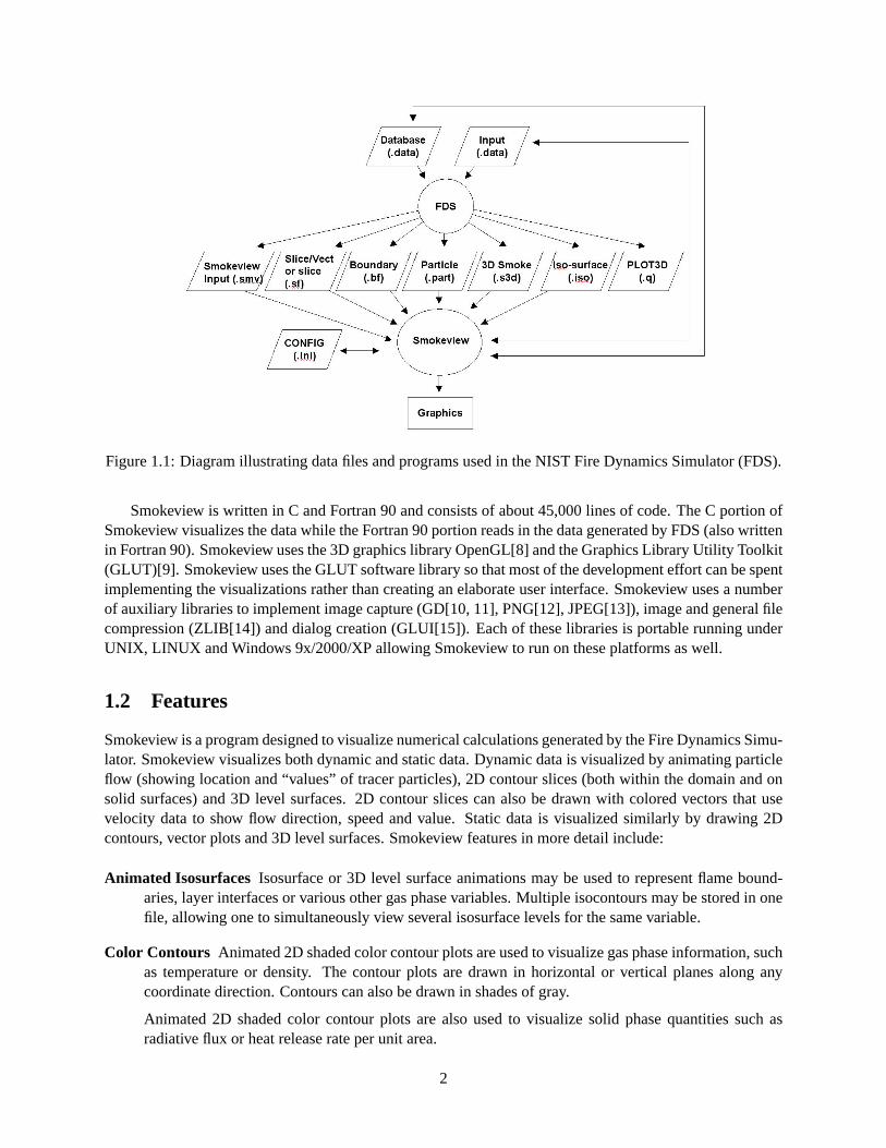
Figure 1.1: Diagram illustrating data files and programs used in the NIST Fire Dynamics Simulator (FDS).
Smokeview is written in C and Fortran 90 and consists of about 45,000 lines of code. The C portion ofSmokeview visualizes the data while the Fortran 90 portion reads in the data generated by FDS (also writtenin Fortran 90). Smokeview uses the 3D graphics library OpenGL[8] and the Graphics Library Utility Toolkit(GLUT)[9]. Smokeview uses the GLUT software library so that most of the development effort can be spentimplementing the visualizations rather than creating an elaborate user interface. Smokeview uses a numberof auxiliary libraries to implement image capture (GD[10, 11], PNG[12], JPEG[13]), image and general filecompression (ZLIB[14]) and dialog creation (GLUI[15]). Each of these libraries is portable running underUNIX, LINUX and Windows 9x/2000/XP allowing Smokeview to run on these platforms as well.
1.2 Features
Smokeview is a program designed to visualize numerical calculations generated by the Fire Dynamics Simu-lator. Smokeview visualizes both dynamic and static data. Dynamic data is visualized by animating particleflow (showing location and “values” of tracer particles), 2D contour slices (both within the domain and onsolid surfaces) and 3D level surfaces. 2D contour slices can also be drawn with colored vectors that usevelocity data to show flow direction, speed and value. Static data is visualized similarly by drawing 2Dcontours, vector plots and 3D level surfaces. Smokeview features in more detail include:
Animated Isosurfaces Isosurface or 3D level surface animations may be used to represent flame bound-aries, layer interfaces or various other gas phase variables. Multiple isocontours may be stored in onefile, allowing one to simultaneously view several isosurface levels for the same variable.
Color Contours Animated 2D shaded color contour plots are used to visualize gas phase information, suchas temperature or density. The contour plots are drawn in horizontal or vertical planes along anycoordinate direction. Contours can also be drawn in shades of gray.
Animated 2D shaded color contour plots are also used to visualize solid phase quantities such asradiative flux or heat release rate per unit area.
2
Animated Flow Vectors Flow vector animations, though similar to color contour animations (the vectorcolors are the same as the corresponding contour colors), are better than solid contour animations athighlighting flow features.
Particle Animations Lagrangian or moving particles can be used to visualize the flow field. Often theseparticles represent smoke or water droplets.
Data Mining The user can analyze and examine the simulated data by altering its appearance to moreeasily identify features and behaviors found in the simulation data. One may flip or reverse the orderof colors in the colorbar and also click in the colorbar and slide the mouse to highlight data values inthe scene. These options may be found underOptions/Shades .
The user may click in the time bar and slide the mouse to change the simulation time displayed. Oneuse for the time bar and color bar selection modes might be to determine when smoke of a particulartemperature enters a room.
Multimesh Geometry Smokeview shows the multi-mesh geometry new in FDS 3, and gives the user con-trol over viewing certain features in a given mesh. Using theLOAD/UNLOAD> MULTI-SLICEmenu item one may now load multiple slices simultaneously. These slices are ones lying in the sameplane (within a grid cell) across multiple meshes.
Scene Clipping It is often difficult to visualize slice or boundary data in complicated geometries due tothe number of obstructed surfaces. Interior portions of the scene may now be seen more easily by“clipping” part of the scene away.
Scene Motion The motion dialog box has been enhanced to allow more precise control of scene movementand orientation. Cursor keys have been mapped to scene translation/rotation to allow easy navigationwithin the scene.
Texture Mapping Jpeg or PNG image files may be applied to a blockage, vent or enclosure boundary. Thisis called texture mapping. This allows one to view Smokeview scenes more realistically. These imagefiles may be obtained from the internet, a digital camera, a scanner or from any other source thatgenerates these file formats. Image files used for texture mapping should be “seamless.” A seamlesstexture as the name suggests is periodic in both horizontal and vertical directions. This is an especiallyimportant feature when textures are tiled or repeated across a blockage surface.
Blockage Editing The Blockage Editing dialog box has been enhanced to allow one to assign materialproperties to selected blockages. Comment labels found in the FDS input file may be viewed or edited.Any text appearing after the closing “/” in an&OBSTline is treated as a comment by Smokeview.
Annotating Cases The two keywords,LABEL andTICKS are used to help document Smokeview output.TheLABEL keyword allows one to place colored labels at specified locations at specified times. TheTICK keyword places equally spaced tick marks between specified bounds. These marks along withLABEL text may be used to document length scales in the scene.
1.3 What’s New
Realistic Smoke Smoke, fire and sprinkler spray are displayed realistically using a series of partially trans-parent planes. The transparencies for smoke are determined by using smoke densities computed byFDS. The transparencies for fire and sprinkler spray are determined by using a heuristic based on heatrelease rate data and water density data, again computed by FDS. Various settings for the 3d smokeoption may be set using the new “3D Smoke” dialog box found in theDialogs menu.
3

Virtual Tour A series of checkpoints or key frames specifying position and view direction may be speci-fied. A smooth path is computed using Kochanek-Bartels splines[16] to go through these key framesso that one may control the position and view direction of an observer as they move through the sim-ulation. One can then see the simulation as the observer would. This option is available under theTour menu item. Existing tours may be edited and new tours may be created using the “Tour”
dialog box found in theDialogs menu. Tour settings are stored in the local configuration file(casename.ini).
Data Chopping - The Set Bounds... dialog box has been enhanced to allow one to chop or hide datain addition to setting bounds. One use of this feature would be to more easily visualize a ceiling jetby hiding ambient temperature data (data below a prescribed temperature).
4
Chapter 2
Getting Started
Smokeview may be obtained at the web sitehttp://fire.nist.gov/smokeview. This site gives links to aSetup program for PC installation. It also contains documentation for Smokeview and FDS, sample FDScalculations, software updates and links for requesting feedback about the software.
After obtaining the setup program, install Smokeview on the PC by either entering the setup programname from the WindowsStart/Run... menu or by double-clicking the downloaded Smokeview setupprogram. The setup program then steps through the program installation. It copies the FDS and Smokeviewexecutables, sample cases, documentation and the Smokeview preference filesmokeview.ini to thedefault directoryC: \nist \fds . The setup program also defines PATH variables and associates the.smvfile extension to the Smokeview program so that one may either type Smokeview at any command lineprompt or double click on any.smv file. Smokeview uses the OpenGL graphics library which is a part ofall Windows distributions except for the first release of Windows 95.
Most computers purchased today are perfectly adequate for running Smokeview with the caveat thatadditional memory should be obtained to bring the memory size up to at least 512 MB in order to dis-play results without “swapping” to disk and hence slowing down the visualizations. For Smokeview itis more important to obtain a fast graphics card than a fast CPU. If the computer will run both FDS andSmokeview then it is important to obtain a fast CPU as well. For example, the townhouse case found athttp://fire.nist.gov/fds/svsamples/thouse3d.data consists of about 180,000 grid cells and is used in many ofthe Figures in this report, required 6.5 hours of CPU time on a 2.8 GHZ Pentium IV Windows XP system.Cases with more grid cells and longer simulation times (the townhouse case simulated 300 S of smoke flow)would clearly benefit from a faster CPU and more memory which are now relatively inexpensive.
5

6
Chapter 3
Basics
Smokeview may be started on the PC by double-clicking the file namedcasename.smv where casenameis the name specified by theCHID keyword defined in the FDS input data file. Menus are accessed byclicking with the right mouse button. TheLoad/Unload menu may be used to read in the data files
to be visualized. TheShow/Hide menu may be used to change how the visualizations are presented.For the most part, the menu choices are self explanatory. Menu items exist for showing and hiding varioussimulation elements, creating screen dumps, obtaining helpetc. Menu items are described in Appendix B.
To use Smokeview from a “command line”, open a DOS (if running on a PC) or UNIX shell, change tothe directory containing the FDS case to be viewed and type:
smokeview casename
where casename is the name specified by theCHID keyword defined in the FDS input data file. Data filesmay be loaded and options may be selected by clicking the right mouse button and picking the appropriatemenu item.
Smokeview opens two windows, one displays the scene and the other displays status information. Clos-ing either window will end the Smokeview session. Multiple copies of Smokeview may be run simultane-ously if the computer has adequate resources.
Normally Smokeview is run during an FDS run, after the run has completed and as an aid in setting upFDS cases by visualizing geometric components such as blockages, vents, sensors,etc. One can then verifythat these modelling elements have been defined and located as intended. One may select the color of theseelements using color parameters in thesmokeview.ini to help distinguish one element from another.Smokeview.ini file entries are described in section D.1.
Although specific video card brands cannot be recommended, they should behigh-enddue to Smoke-view’s intensive graphics requirements. These requirements will only increase in the future as more featuresare added. A video card designed to perform well for “fancy” computer games should do well for Smoke-view. Some apparent bugs in Smokeview have been found to be the result of problems found in video cardson older computers.
3.1 Manipulating the Scene
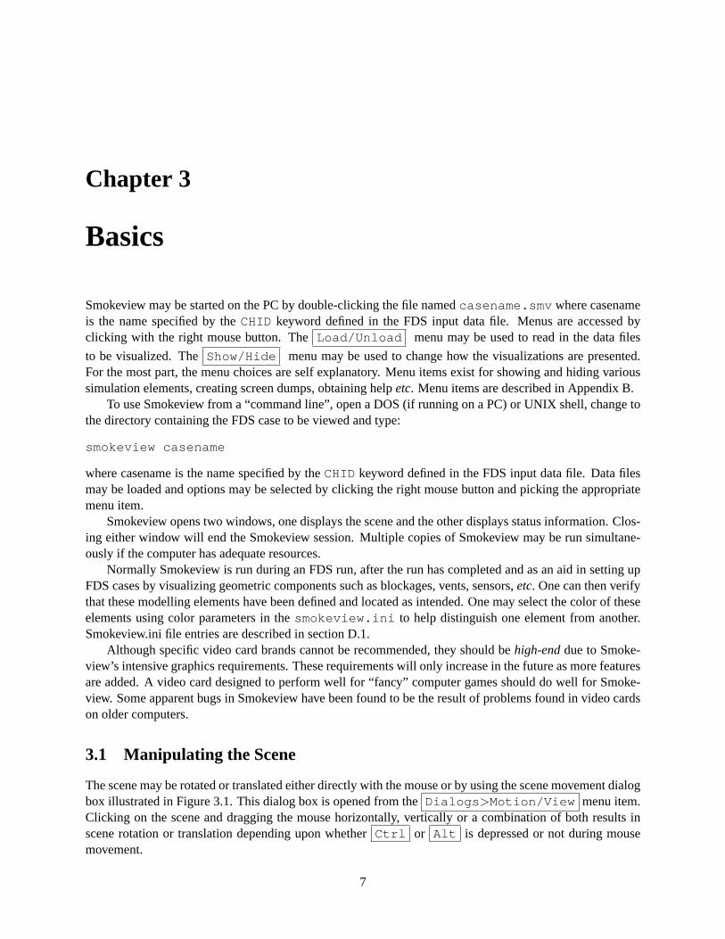
The scene may be rotated or translated either directly with the mouse or by using the scene movement dialogbox illustrated in Figure 3.1. This dialog box is opened from theDialogs >Motion/View menu item.Clicking on the scene and dragging the mouse horizontally, vertically or a combination of both results inscene rotation or translation depending upon whetherCtrl or Alt is depressed or not during mousemovement.
7
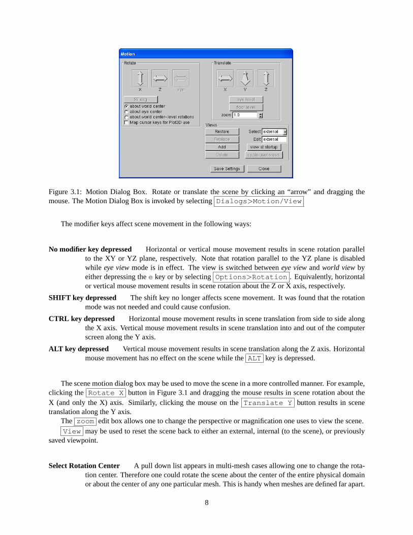
Figure 3.1: Motion Dialog Box. Rotate or translate the scene by clicking an “arrow” and dragging themouse. The Motion Dialog Box is invoked by selectingDialogs >Motion/View
The modifier keys affect scene movement in the following ways:
No modifier key depressed Horizontal or vertical mouse movement results in scene rotation parallelto the XY or YZ plane, respectively. Note that rotation parallel to the YZ plane is disabledwhile eye viewmode is in effect. The view is switched betweeneye viewandworld viewbyeither depressing thee key or by selectingOptions >Rotation . Equivalently, horizontalor vertical mouse movement results in scene rotation about the Z or X axis, respectively.
SHIFT key depressed The shift key no longer affects scene movement. It was found that the rotationmode was not needed and could cause confusion.
CTRL key depressed Horizontal mouse movement results in scene translation from side to side alongthe X axis. Vertical mouse movement results in scene translation into and out of the computerscreen along the Y axis.
ALT key depressed Vertical mouse movement results in scene translation along the Z axis. Horizontalmouse movement has no effect on the scene while theALT key is depressed.
The scene motion dialog box may be used to move the scene in a more controlled manner. For example,clicking the Rotate X button in Figure 3.1 and dragging the mouse results in scene rotation about theX (and only the X) axis. Similarly, clicking the mouse on theTranslate Y button results in scenetranslation along the Y axis.
The zoom edit box allows one to change the perspective or magnification one uses to view the scene.View may be used to reset the scene back to either an external, internal (to the scene), or previously
saved viewpoint.
Select Rotation Center A pull down list appears in multi-mesh cases allowing one to change the rota-tion center. Therefore one could rotate the scene about the center of the entire physical domainor about the center of any one particular mesh. This is handy when meshes are defined far apart.
8
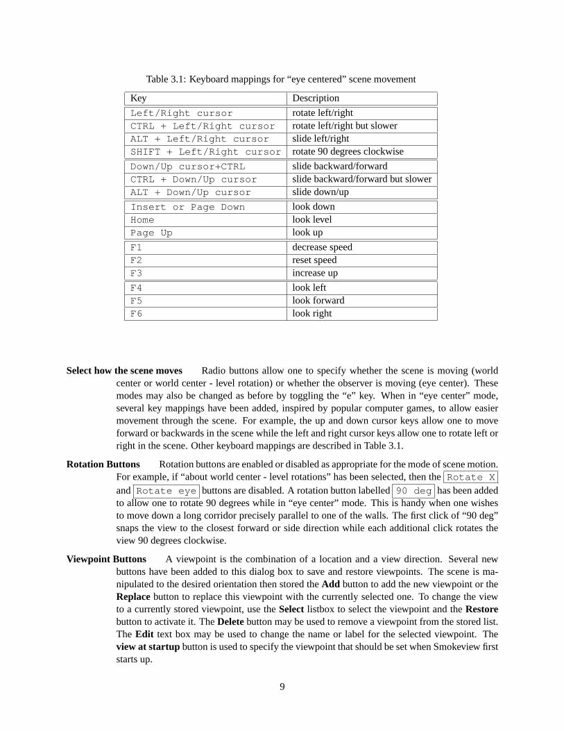
Table 3.1: Keyboard mappings for “eye centered” scene movement
Key Description
Left/Right cursor rotate left/rightCTRL + Left/Right cursor rotate left/right but slowerALT + Left/Right cursor slide left/rightSHIFT + Left/Right cursor rotate 90 degrees clockwise
Down/Up cursor+CTRL slide backward/forwardCTRL + Down/Up cursor slide backward/forward but slowerALT + Down/Up cursor slide down/up
Insert or Page Down look downHome look levelPage Up look up
F1 decrease speedF2 reset speedF3 increase up
F4 look leftF5 look forwardF6 look right
Select how the scene moves Radio buttons allow one to specify whether the scene is moving (worldcenter or world center - level rotation) or whether the observer is moving (eye center). Thesemodes may also be changed as before by toggling the “e” key. When in “eye center” mode,several key mappings have been added, inspired by popular computer games, to allow easiermovement through the scene. For example, the up and down cursor keys allow one to moveforward or backwards in the scene while the left and right cursor keys allow one to rotate left orright in the scene. Other keyboard mappings are described in Table 3.1.
Rotation Buttons Rotation buttons are enabled or disabled as appropriate for the mode of scene motion.For example, if “about world center - level rotations” has been selected, then theRotate X
and Rotate eye buttons are disabled. A rotation button labelled90 deg has been addedto allow one to rotate 90 degrees while in “eye center” mode. This is handy when one wishesto move down a long corridor precisely parallel to one of the walls. The first click of “90 deg”snaps the view to the closest forward or side direction while each additional click rotates theview 90 degrees clockwise.
Viewpoint Buttons A viewpoint is the combination of a location and a view direction. Several newbuttons have been added to this dialog box to save and restore viewpoints. The scene is ma-nipulated to the desired orientation then stored theAdd button to add the new viewpoint or theReplacebutton to replace this viewpoint with the currently selected one. To change the viewto a currently stored viewpoint, use theSelectlistbox to select the viewpoint and theRestorebutton to activate it. TheDeletebutton may be used to remove a viewpoint from the stored list.The Edit text box may be used to change the name or label for the selected viewpoint. Theview at startup button is used to specify the viewpoint that should be set when Smokeview firststarts up.
9
5.0 s 10.0 s
30.0 s 60.0 s
Figure 3.2: Cross section of a townhouse showing first and second floor. Particle file snapshots at four timesduring the simulation of a townhouse kitchen fire.
3.2 Tracer Particles - Particle Files
FDS generates several data files visualized by Smokeview. Each file type may be loaded or unloaded us-ing the Load/Unload menu described in Appendix B.2. Visualizations produced by these data files aredescribed below. The format used to store each of the data files is given in Appendix D.3. The FDS input datafile used to generate the following examples may be found at http://fire.nist.gov/fds/svsamples/thouse3d.data.
Particle files contain the locations of tracer particles used to visualize the flow field. Colors are selectedfrom a user definable color palette defined using theCOLORBARkeyword documented in Appendix D.1.Figure 3.2 shows several snapshots of a developing kitchen fire visualized by using particles where particlesare colored black. If present, sprinkler water droplets would be colored blue. Particles are stored in filesending with the extension.part and are displayed by selecting the entry from theLoad/Unload menu.
3.3 3D Smoke
Visualizing smoke realistically is a daunting challenge for at least three reasons. First, the storage require-ments for describing smoke can easily exceed the disk capacities of present 32 bit operating systems suchas Linux,i.e. file sizes can easily exceed 2 gigabytes. Second, the computation required both by the CPUand the video card to display each frame can easily exceed 0.1 s, the time corresponding to a 10 frame/sdisplay rate. Third, the physics required to describe smoke and its interactions with itself and surroundinglight sources is complex and computationally intensive. Therefore, approximations and simplifications arerequired to display smoke rapidly.
Smoke visualization techniques such as tracer particles or shaded 2D contours are useful for quantitative
10
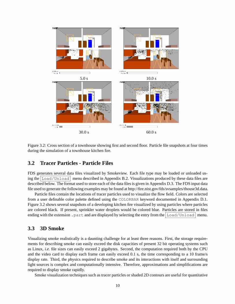
5.0 s 10.0 s
30.0 s 60.0 s
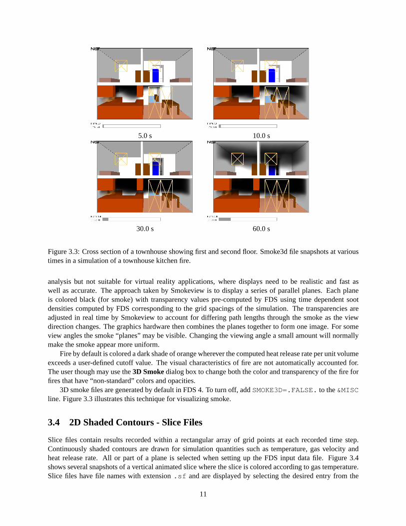
Figure 3.3: Cross section of a townhouse showing first and second floor. Smoke3d file snapshots at varioustimes in a simulation of a townhouse kitchen fire.
analysis but not suitable for virtual reality applications, where displays need to be realistic and fast aswell as accurate. The approach taken by Smokeview is to display a series of parallel planes. Each planeis colored black (for smoke) with transparency values pre-computed by FDS using time dependent sootdensities computed by FDS corresponding to the grid spacings of the simulation. The transparencies areadjusted in real time by Smokeview to account for differing path lengths through the smoke as the viewdirection changes. The graphics hardware then combines the planes together to form one image. For someview angles the smoke “planes” may be visible. Changing the viewing angle a small amount will normallymake the smoke appear more uniform.
Fire by default is colored a dark shade of orange wherever the computed heat release rate per unit volumeexceeds a user-defined cutoff value. The visual characteristics of fire are not automatically accounted for.The user though may use the3D Smokedialog box to change both the color and transparency of the fire forfires that have “non-standard” colors and opacities.
3D smoke files are generated by default in FDS 4. To turn off, addSMOKE3D=.FALSE.to the&MISCline. Figure 3.3 illustrates this technique for visualizing smoke.
3.4 2D Shaded Contours - Slice Files
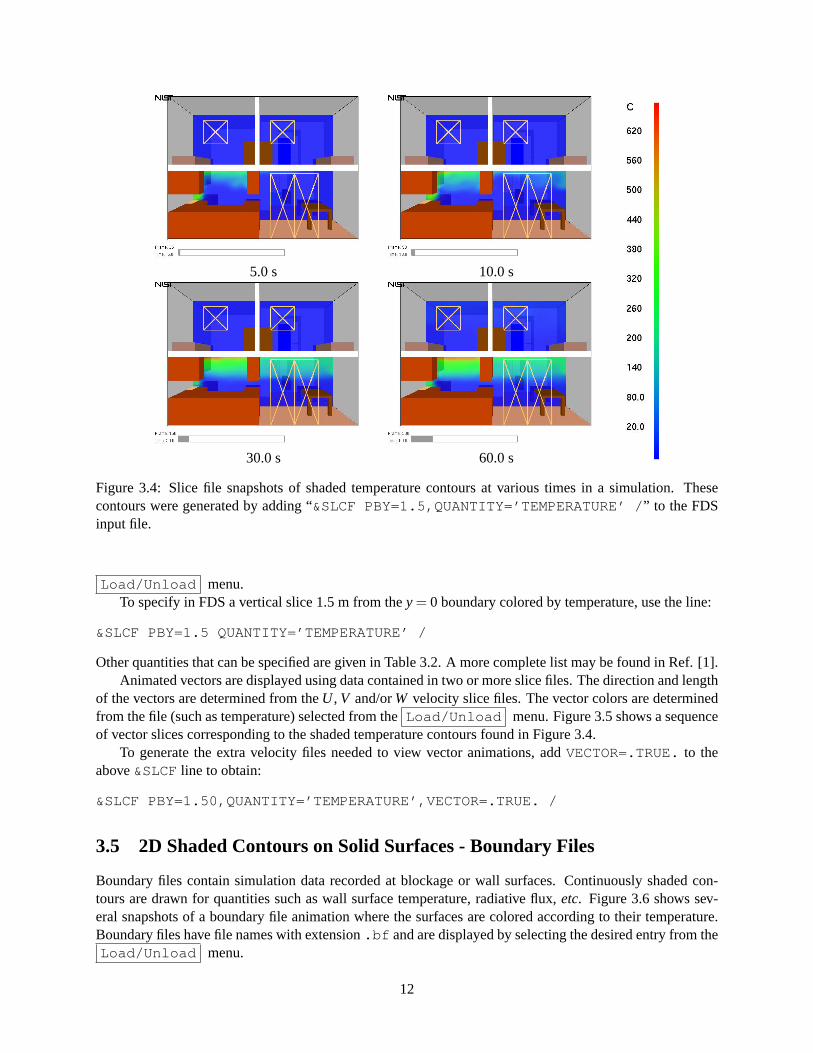
Slice files contain results recorded within a rectangular array of grid points at each recorded time step.Continuously shaded contours are drawn for simulation quantities such as temperature, gas velocity andheat release rate. All or part of a plane is selected when setting up the FDS input data file. Figure 3.4shows several snapshots of a vertical animated slice where the slice is colored according to gas temperature.Slice files have file names with extension.sf and are displayed by selecting the desired entry from the
11
5.0 s 10.0 s
30.0 s 60.0 s
Figure 3.4: Slice file snapshots of shaded temperature contours at various times in a simulation. Thesecontours were generated by adding “&SLCF PBY=1.5,QUANTITY=’TEMPERATURE’ / ” to the FDSinput file.
Load/Unload menu.To specify in FDS a vertical slice 1.5 m from they = 0 boundary colored by temperature, use the line:
&SLCF PBY=1.5 QUANTITY=’TEMPERATURE’ /
Other quantities that can be specified are given in Table 3.2. A more complete list may be found in Ref. [1].Animated vectors are displayed using data contained in two or more slice files. The direction and length
of the vectors are determined from theU , V and/orW velocity slice files. The vector colors are determinedfrom the file (such as temperature) selected from theLoad/Unload menu. Figure 3.5 shows a sequenceof vector slices corresponding to the shaded temperature contours found in Figure 3.4.
To generate the extra velocity files needed to view vector animations, addVECTOR=.TRUE. to theabove&SLCFline to obtain:
&SLCF PBY=1.50,QUANTITY=’TEMPERATURE’,VECTOR=.TRUE. /
3.5 2D Shaded Contours on Solid Surfaces - Boundary Files
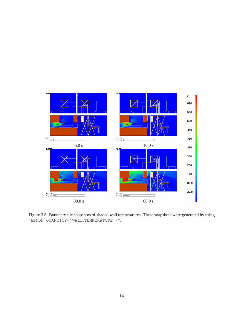
Boundary files contain simulation data recorded at blockage or wall surfaces. Continuously shaded con-tours are drawn for quantities such as wall surface temperature, radiative flux,etc. Figure 3.6 shows sev-eral snapshots of a boundary file animation where the surfaces are colored according to their temperature.Boundary files have file names with extension.bf and are displayed by selecting the desired entry from theLoad/Unload menu.
12

Table 3.2: Some output quantities used to generate slice and Plot3D visualizations. A more complete listmay be found in Ref.[1]
Quantity Description Units
DENSITY density kg/m3
TEMPERATURE gas temperature ◦CU-VELOCITY velocity component m/sV-VELOCITY velocity component m/sW-VELOCITY velocity component m/sVELOCITY velocity magnitude m/s
5.0 s 10.0 s
30.0 s 60.0 s
Figure 3.5: Vector slice file snapshots of shaded vector plots. These vector plots were generated by using“&SLCF PBY=1.5,QUANTITY=’TEMPERATURE’,VECTOR=.TRUE. / ”.
13
5.0 s 10.0 s
30.0 s 60.0 s
Figure 3.6: Boundary file snapshots of shaded wall temperatures. These snapshots were generated by using“&BNDF QUANTITY=’WALLTEMPERATURE’/”.
14
Table 3.3: Some output quantities used to generate boundary file visualizations. A more complete list maybe found in Ref.[1]
Quantity Description Units
RADIATIVE FLUX radiative flux kW/m2
CONVECTIVEFLUX convective flux kW/m2
WALLTEMPERATURE wall temperature ◦C
A boundary file containing wall temperature data may be generated by using:
&BNDF ’WALL_TEMPERATURE’ /
Loading a boundary file is a memory intensive operation. The entire boundary file is read in to determinethe minimum and maximum data values. These bounds are then used to convert four byte floats to one bytecolor indices. To drastically reduce the memory requirements, simply specify the minimum and maximumdata bounds using theSet Bounds dialog box. This should be done before loading the boundary filedata. When this is done, memory for the boundary file data is allocated for only one time step rather thanfor all time steps.
Table 3.3 gives other quantities that can be specified on a&BNDFline. A more complete list of quantitiesis given in Ref. [1].
3.6 3D Contours - Isosurface Files
The surface where a quantity such as temperature attains a given value is called an isosurface. An isosurfaceis also called a level surface or 3D contour. Isosurface files contain data specifying isosurface locations fora given quantity at one or more levels. These surfaces are represented as triangles. Isosurface files havefile names with extension .iso and are displayed by selecting the desired entry from theLoad/Unloadmenu.
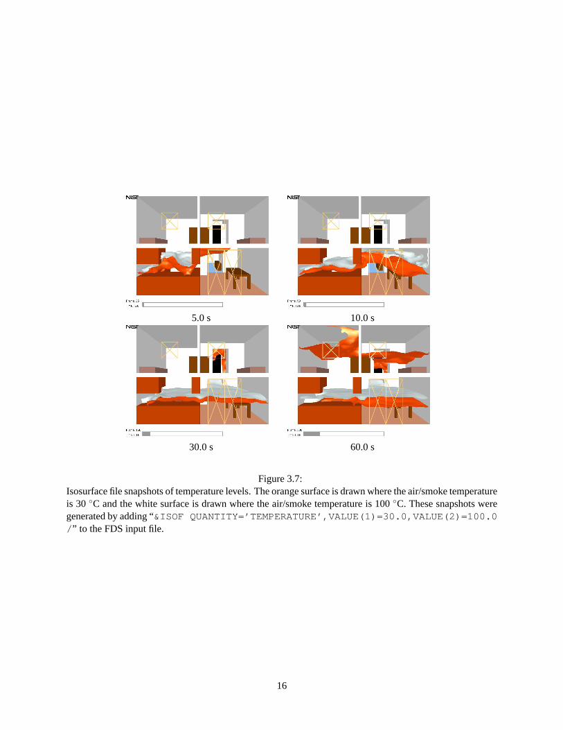
Isosurfaces are specified in the FDS input file with the&ISOF keyword. To specify isosurfaces fortemperatures of 30◦C and 100◦C as illustrated in Figure 3.7 add the line:
&ISOF QUANTITY=’TEMPERATURE’,VALUE(1)=30.0,VALUE(2)=100.0 /
to the FDS input file. Other quantities may be specified using values given in Table 3.2. A more completelist may be found in Ref. [1]
3.7 Static Data - Plot3D Files
Data stored in Plot3D files use a format developed by NASA [17] and are used by many CFD programs forrepresenting simulation results. Plot3D files store five data values at each grid cell. FDS uses Plot3D filesto store temperature, three components of velocity (U, V, W) and heat release rate. Other quantities may bestored if desired.
An FDS simulation will typically create Plot3D files at several specified times throughout the simulation.Plot3D data is visualized in three ways: as 2D contours, vector plots and isosurfaces. Figure 3.8a shows anexample of a 2D Plot3D contour. Vector plots may be viewed if one or more of the U,V and W velocitycomponents are stored in the Plot3D file. The vector length and direction show the direction and relativespeed of the fluid flow. The vector colors show a scalar fluid quantity such as temperature. Figure 3.8b
15
5.0 s 10.0 s
30.0 s 60.0 s
Figure 3.7:Isosurface file snapshots of temperature levels. The orange surface is drawn where the air/smoke temperatureis 30 ◦C and the white surface is drawn where the air/smoke temperature is 100◦C. These snapshots weregenerated by adding “&ISOF QUANTITY=’TEMPERATURE’,VALUE(1)=30.0,VALUE(2)=100.0/ ” to the FDS input file.
16
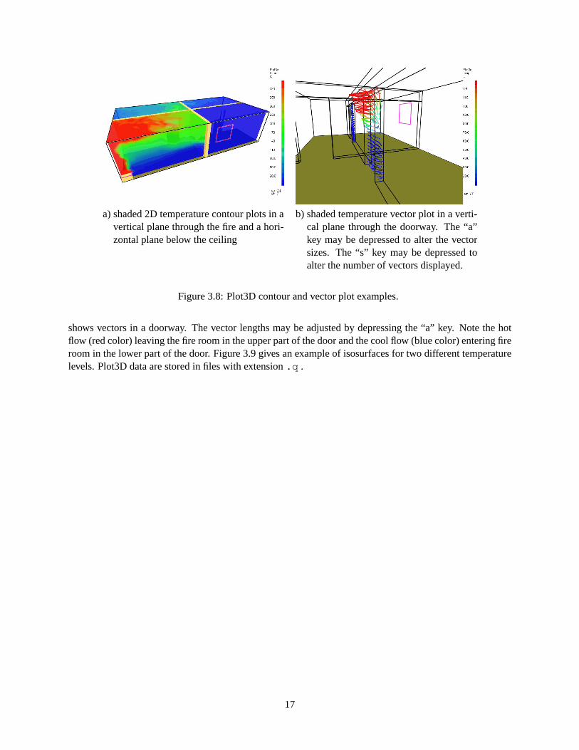
a) shaded 2D temperature contour plots in avertical plane through the fire and a hori-zontal plane below the ceiling
b) shaded temperature vector plot in a verti-cal plane through the doorway. The “a”key may be depressed to alter the vectorsizes. The “s” key may be depressed toalter the number of vectors displayed.
Figure 3.8: Plot3D contour and vector plot examples.
shows vectors in a doorway. The vector lengths may be adjusted by depressing the “a” key. Note the hotflow (red color) leaving the fire room in the upper part of the door and the cool flow (blue color) entering fireroom in the lower part of the door. Figure 3.9 gives an example of isosurfaces for two different temperaturelevels. Plot3D data are stored in files with extension.q .
17
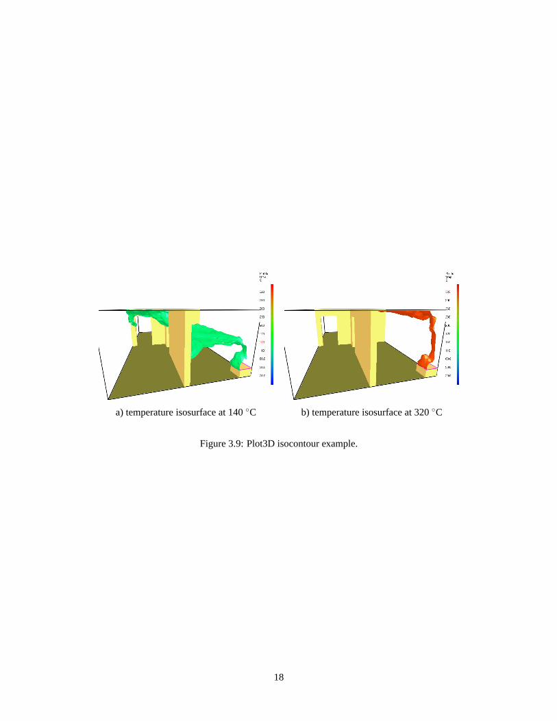
a) temperature isosurface at 140◦C b) temperature isosurface at 320◦C
Figure 3.9: Plot3D isocontour example.
18
Chapter 4
Advanced Features
4.1 Manipulating the Scene Automatically - The Touring Option
The touring option allows one to specify arbitrary paths or tours through or around a Smokeview scene.One may then view the scenario from the vantage point of an observer moving along one of these paths.Alternatively, one may observe the motion along all of the paths simultaneously from an external vantagepoint. These paths may be used to represent the movement of building occupants or first responders duringa fire incident, or to highlight key portions or features of a scenario during presentations. A tour may alsobe used to observe time dependent portions of the scenario such as blockage/vent opening and closings.The default view direction is towards the direction of motion. The view direction and path tension may bechanged with theAdvanced Settingsdialog box.
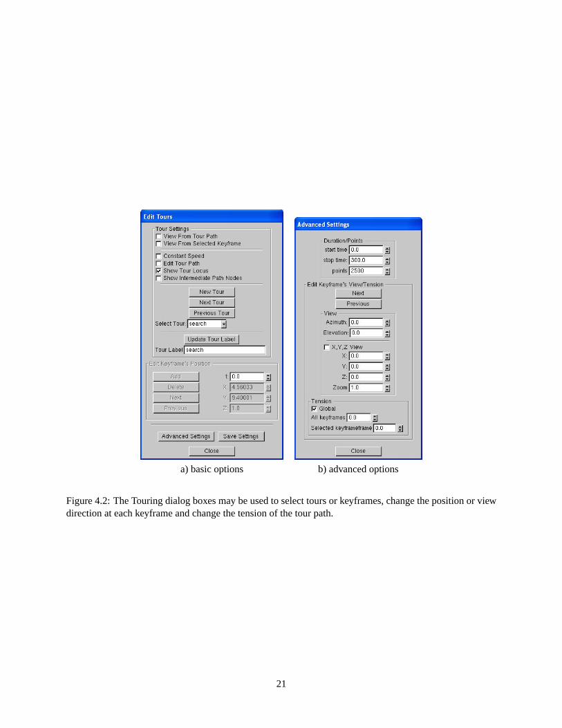
When Smokeview starts up it creates a tour, called the “circle tour” which surrounds the scene. The“circle” tour and a user defined tour are illustrated in Figure 4.1. The circle tour is similar to theTourmenu option found in earlier versions of Smokeview. The user may modify the “circle” tour or define theirown tours by using theTour dialog box illustrated in Figure 4.2. The user places several points or keyframesin or around the scene. Smokeview creates a smooth path going through these points.
Tour Settings An existing tour may be modified by selecting it from theSelect tour: listbox found in theTour dialog box. A new tour may be created by clicking theAdd Tour button. A newly created tour goesthrough the middle of the Smokeview scene starting at the front left and finishing at the back right. A tourmay also be modified by editing the text entries found in the “local” preference file, casename.ini under theTOUR keyword.
The speed traversed along the tour is determined by the time value assigned to each keyframe. If theConstant Speedcheckbox is checked then these times are determined given the distance between keyframesand the velocity required to traverse the entire path in the specified time as given by the “start time” and“stop time” entries found in theAdvanced Settingsdialog box.
Three different methods for viewing the scene may be selected. To view the scene from the point ofview of the selected tour, check theView From Tour Path checkbox. To view the scene from a keyframe(to see the effect of editing changes), select theView From Selected Keyframecheckbox. Uncheckingthese boxes returns control of scene movement to the user.
Keyframe Settings A keyframe may be selected for editing by either clicking it with the mouse or byusing theNext or Previousbuttons. Keyframe positions may then be modified by changing data in the t, X,Y or Z edit boxes. A different view direction may be selected using theAdvanced Settingsdialog box.
19
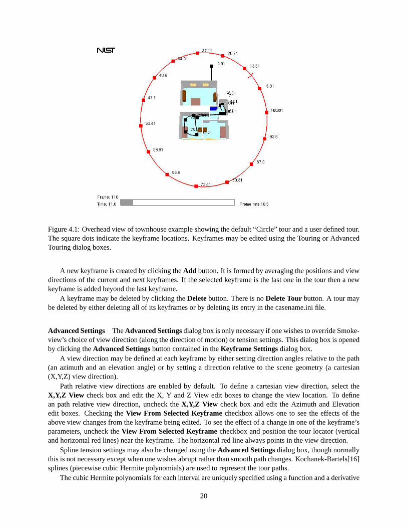
Figure 4.1: Overhead view of townhouse example showing the default “Circle” tour and a user defined tour.The square dots indicate the keyframe locations. Keyframes may be edited using the Touring or AdvancedTouring dialog boxes.
A new keyframe is created by clicking theAdd button. It is formed by averaging the positions and viewdirections of the current and next keyframes. If the selected keyframe is the last one in the tour then a newkeyframe is added beyond the last keyframe.
A keyframe may be deleted by clicking theDeletebutton. There is noDelete Tour button. A tour maybe deleted by either deleting all of its keyframes or by deleting its entry in the casename.ini file.
Advanced Settings TheAdvanced Settingsdialog box is only necessary if one wishes to override Smoke-view’s choice of view direction (along the direction of motion) or tension settings. This dialog box is openedby clicking theAdvanced Settingsbutton contained in theKeyframe Settingsdialog box.
A view direction may be defined at each keyframe by either setting direction angles relative to the path(an azimuth and an elevation angle) or by setting a direction relative to the scene geometry (a cartesian(X,Y,Z) view direction).
Path relative view directions are enabled by default. To define a cartesian view direction, select theX,Y,Z View check box and edit the X, Y and Z View edit boxes to change the view location. To definean path relative view direction, uncheck theX,Y,Z View check box and edit the Azimuth and Elevationedit boxes. Checking theView From Selected Keyframecheckbox allows one to see the effects of theabove view changes from the keyframe being edited. To see the effect of a change in one of the keyframe’sparameters, uncheck theView From Selected Keyframecheckbox and position the tour locator (verticaland horizontal red lines) near the keyframe. The horizontal red line always points in the view direction.
Spline tension settings may also be changed using theAdvanced Settingsdialog box, though normallythis is not necessary except when one wishes abrupt rather than smooth path changes. Kochanek-Bartels[16]splines (piecewise cubic Hermite polynomials) are used to represent the tour paths.
The cubic Hermite polynomials for each interval are uniquely specified using a function and a derivative
20
a) basic options b) advanced options
Figure 4.2: The Touring dialog boxes may be used to select tours or keyframes, change the position or viewdirection at each keyframe and change the tension of the tour path.
21
a) Initial tour b) First and last step set with 5 keyframes
c) All keyframe positions set (tension=0.0) d) Tension set to 0.75
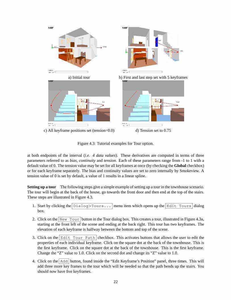
Figure 4.3: Tutorial examples for Tour option.
at both endpoints of the interval (i.e. 4 data values). These derivatives are computed in terms of threeparameters referred to asbias, continuityandtension. Each of these parameters range from -1 to 1 with adefault value of 0. The tension value may be set for all keyframes at once (by checking theGlobal checkbox)or for each keyframe separately. The bias and continuity values are set to zero internally by Smokeview. Atension value of 0 is set by default, a value of 1 results in a linear spline.
Setting up a tour The following steps give a simple example of setting up a tour in the townhouse scenario.The tour will begin at the back of the house, go towards the front door and then end at the top of the stairs.These steps are illustrated in Figure 4.3.
1. Start by clicking theDialog >Tours... menu item which opens up theEdit Tours dialogbox.
2. Click on the New Tour button in the Tour dialog box. This creates a tour, illustrated in Figure 4.3a,starting at the front left of the scene and ending at the back right. This tour has two keyframes. Theelevation of each keyframe is halfway between the bottom and top of the scene.
3. Click on the Edit Tour Path checkbox. This activates buttons that allows the user to edit theproperties of each individual keyframe. Click on the square dot at the back of the townhouse. This isthe first keyframe. Click on the square dot at the back of the townhouse. This is the first keyframe.Change the “Z” value to 1.0. Click on the second dot and change its “Z” value to 1.0.
4. Click on the Add button, found inside the “Edit Keyframe’s Position” panel, three times. This willadd three more key frames to the tour which will be needed so that the path bends up the stairs. Youshould now have five keyframes.
22
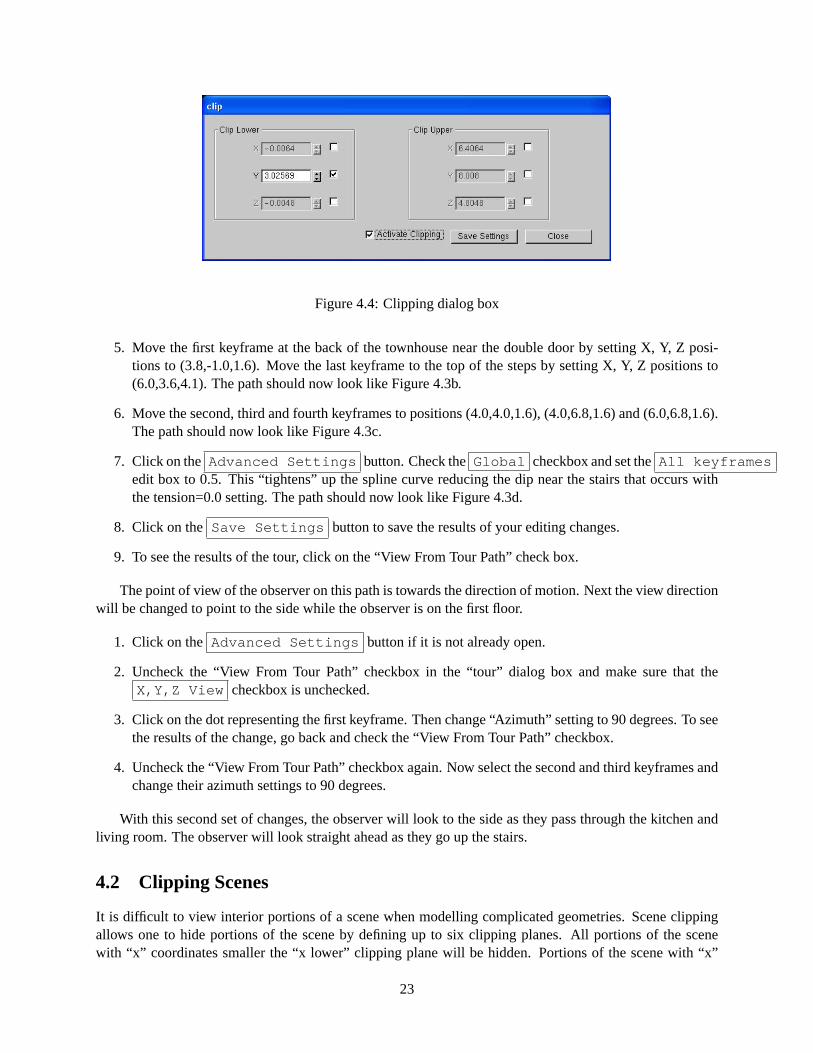
Figure 4.4: Clipping dialog box
5. Move the first keyframe at the back of the townhouse near the double door by setting X, Y, Z posi-tions to (3.8,-1.0,1.6). Move the last keyframe to the top of the steps by setting X, Y, Z positions to(6.0,3.6,4.1). The path should now look like Figure 4.3b.
6. Move the second, third and fourth keyframes to positions (4.0,4.0,1.6), (4.0,6.8,1.6) and (6.0,6.8,1.6).The path should now look like Figure 4.3c.
7. Click on the Advanced Settings button. Check theGlobal checkbox and set theAll keyframesedit box to 0.5. This “tightens” up the spline curve reducing the dip near the stairs that occurs withthe tension=0.0 setting. The path should now look like Figure 4.3d.
8. Click on the Save Settings button to save the results of your editing changes.
9. To see the results of the tour, click on the “View From Tour Path” check box.
The point of view of the observer on this path is towards the direction of motion. Next the view directionwill be changed to point to the side while the observer is on the first floor.
1. Click on the Advanced Settings button if it is not already open.
2. Uncheck the “View From Tour Path” checkbox in the “tour” dialog box and make sure that theX,Y,Z View checkbox is unchecked.
3. Click on the dot representing the first keyframe. Then change “Azimuth” setting to 90 degrees. To seethe results of the change, go back and check the “View From Tour Path” checkbox.
4. Uncheck the “View From Tour Path” checkbox again. Now select the second and third keyframes andchange their azimuth settings to 90 degrees.
With this second set of changes, the observer will look to the side as they pass through the kitchen andliving room. The observer will look straight ahead as they go up the stairs.
4.2 Clipping Scenes
It is difficult to view interior portions of a scene when modelling complicated geometries. Scene clippingallows one to hide portions of the scene by defining up to six clipping planes. All portions of the scenewith “x” coordinates smaller the “x lower” clipping plane will be hidden. Portions of the scene with “x”
23
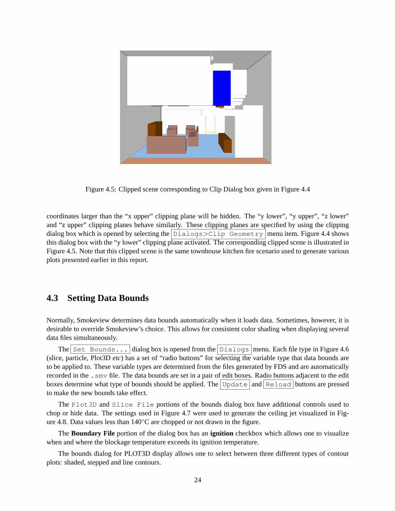
Figure 4.5: Clipped scene corresponding to Clip Dialog box given in Figure 4.4
coordinates larger than the “x upper” clipping plane will be hidden. The “y lower”, “y upper”, “z lower”and “z upper” clipping planes behave similarly. These clipping planes are specified by using the clippingdialog box which is opened by selecting theDialogs >Clip Geometry menu item. Figure 4.4 showsthis dialog box with the “y lower” clipping plane activated. The corresponding clipped scene is illustrated inFigure 4.5. Note that this clipped scene is the same townhouse kitchen fire scenario used to generate variousplots presented earlier in this report.
4.3 Setting Data Bounds
Normally, Smokeview determines data bounds automatically when it loads data. Sometimes, however, it isdesirable to override Smokeview’s choice. This allows for consistent color shading when displaying severaldata files simultaneously.
The Set Bounds... dialog box is opened from theDialogs menu. Each file type in Figure 4.6(slice, particle, Plot3Detc) has a set of “radio buttons” for selecting the variable type that data bounds areto be applied to. These variable types are determined from the files generated by FDS and are automaticallyrecorded in the.smv file. The data bounds are set in a pair of edit boxes. Radio buttons adjacent to the editboxes determine what type of bounds should be applied. TheUpdate and Reload buttons are pressedto make the new bounds take effect.
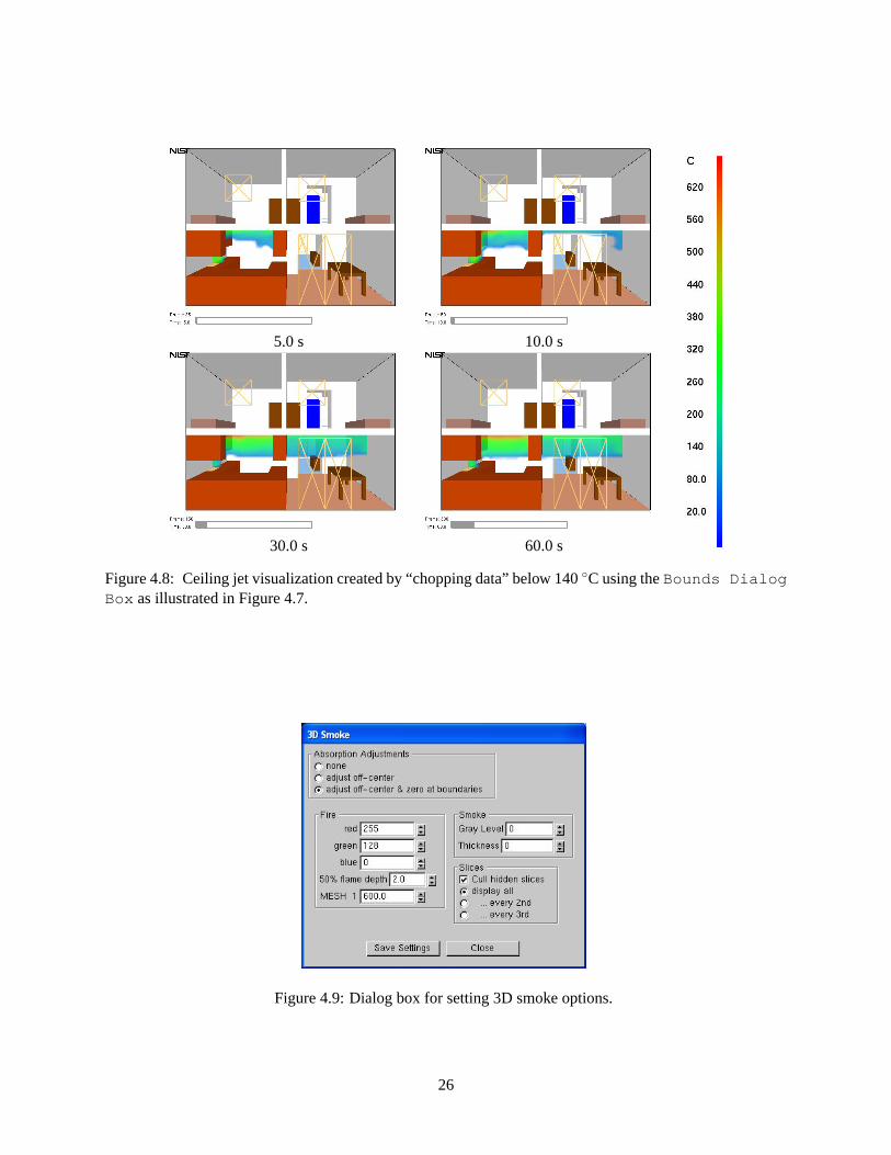
The Plot3D andSlice File portions of the bounds dialog box have additional controls used tochop or hide data. The settings used in Figure 4.7 were used to generate the ceiling jet visualized in Fig-ure 4.8. Data values less than 140◦C are chopped or not drawn in the figure.
TheBoundary File portion of the dialog box has anignition checkbox which allows one to visualizewhen and where the blockage temperature exceeds its ignition temperature.
The bounds dialog for PLOT3D display allows one to select between three different types of contourplots: shaded, stepped and line contours.
24
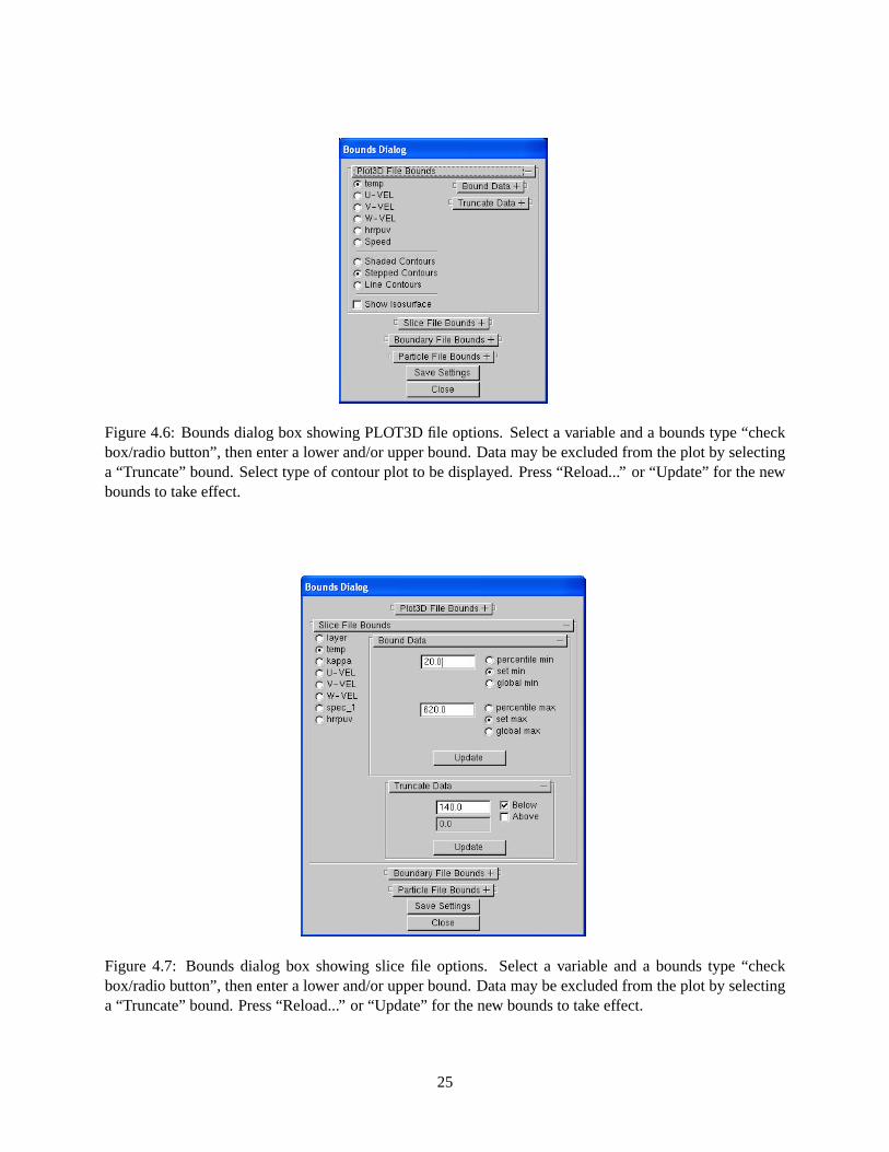
Figure 4.6: Bounds dialog box showing PLOT3D file options. Select a variable and a bounds type “checkbox/radio button”, then enter a lower and/or upper bound. Data may be excluded from the plot by selectinga “Truncate” bound. Select type of contour plot to be displayed. Press “Reload...” or “Update” for the newbounds to take effect.
Figure 4.7: Bounds dialog box showing slice file options. Select a variable and a bounds type “checkbox/radio button”, then enter a lower and/or upper bound. Data may be excluded from the plot by selectinga “Truncate” bound. Press “Reload...” or “Update” for the new bounds to take effect.
25
5.0 s 10.0 s
30.0 s 60.0 s
Figure 4.8: Ceiling jet visualization created by “chopping data” below 140◦C using theBounds DialogBox as illustrated in Figure 4.7.
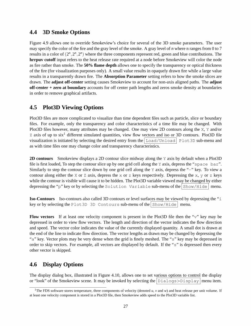
Figure 4.9: Dialog box for setting 3D smoke options.
26
4.4 3D Smoke Options
Figure 4.9 allows one to override Smokeview’s choice for several of the 3D smoke parameters. The usermay specify the color of the fire and the gray level of the smoke. A gray level ofn where n ranges from 0 to 7results in a color of(2n,2n,2n) where the three components represent red, green and blue contributions. Thehrrpuv cutoff input refers to the heat release rate required at a node before Smokeview will color the nodeas fire rather than smoke. The50% flame depthallows one to specify the transparency or optical thicknessof the fire (for visualization purposes only). A small value results in opaquely drawn fire while a large valueresults in a transparently drawn fire. TheAbsorption Parameter setting refers to how the smoke slices aredrawn. Theadjust off-center setting causes Smokeview to account for non-axis aligned paths. Theadjustoff-center + zero at boundaryaccounts for off center path lengths and zeros smoke density at boundariesin order to remove graphical artifacts.
4.5 Plot3D Viewing Options
Plot3D files are more complicated to visualize than time dependent files such as particle, slice or boundaryfiles. For example, only the transparency and color characteristics of a time file may be changed. WithPlot3D files however, many attributes may be changed. One may view 2D contours along theX, Y and/orZ axis of up to six1 different simulated quantities, view flow vectors and iso or 3D contours. Plot3D filevisualization is initiated by selecting the desired entry from theLoad/Unload Plot3D sub-menu andas with time files one may change color and transparency characteristics.
2D contours Smokeview displays a 2D contour slice midway along theY axis by default when a Plot3Dfile is first loaded, To step the contour slice up by one grid cell along theY axis, depress the “space bar ”.Similarly to step the contour slice down by one grid cell along theY axis, depress the “- ” key. To view acontour along either theX or Z axis, depress thex or z keys respectively. Depressing thex , y or z keyswhile the contour is visible will cause it to be hidden. The Plot3D variable viewed may be changed by eitherdepressing the “p” key or by selecting theSolution Variable sub-menu of theShow/Hide menu.
Iso-Contours Iso-contours also called 3D contours or level surfaces may be viewed by depressing the “ikey or by selecting thePlot3D 3D Contours sub-menu of theShow/Hide menu.
Flow vectors If at least one velocity component is present in the Plot3D file then the “v ” key may bedepressed in order to view flow vectors. The length and direction of the vector indicates the flow directionand speed. The vector color indicates the value of the currently displayed quantity. A small dot is drawn atthe end of the line to indicate flow direction. The vector lengths as drawn may be changed by depressing the“a” key. Vector plots may be very dense when the grid is finely meshed. The “s ” key may be depressed inorder to skip vectors. For example, all vectors are displayed by default. If the “s ” is depressed then everyother vector is skipped.
4.6 Display Options
The display dialog box, illustrated in Figure 4.10, allows one to set various options to control the displayor “look” of the Smokeview scene. It may be invoked by selecting theDialogs >Display menu item.
1The FDS software stores temperature, three components of velocity (denotedu, v andw) and heat release per unit volume. Ifat least one velocity component is stored in a Plot3D file, then Smokeview adds speed to the Plot3D variable list.
27
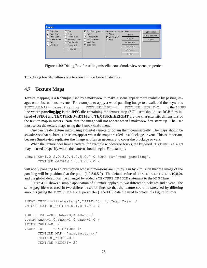
Figure 4.10: Dialog Box for setting miscellaneous Smokeview scene properties
This dialog box also allows one to show or hide loaded data files.
4.7 Texture Maps
Texture mapping is a technique used by Smokeview to make a scene appear more realistic by pasting im-ages onto obstructions or vents. For example, to apply a wood paneling image to a wall, add the keywordsTEXTUREMAP=’paneling.jpg’, TEXTURE WIDTH=1., TEXTURE HEIGHT=2. to the&SURFline wherepaneling.jpg is the JPEG file containing the texture map (SGI users should use RGB files in-stead of JPEG) andTEXTURE WIDTH andTEXTURE HEIGHT are the characteristic dimensions ofthe texture map in meters. Note that the image will not appear when Smokeview first starts up. The usermust select the texture maps using theShow/Hide menu.
One can create texture maps using a digital camera or obtain them commercially. The maps should beseamlessso that no breaks or seams appear when the maps are tiled on a blockage or vent. This is important,because Smokeview replicates the image as often as necessary to cover the blockage or vent.
When the texture does have a pattern, for example windows or bricks, the keywordTEXTUREORIGINmay be used to specify where the pattern should begin. For example,
&OBST XB=1.0,2.0,3.0,4.0,5.0,7.0,SURF_ID=’wood paneling’,TEXTURE_ORIGIN=1.0,3.0,5.0 /
will apply paneling to an obstruction whose dimensions are 1 m by 1 m by 2 m, such that the image of thepaneling will be positioned at the point (1.0,3.0,5.0). The default value ofTEXTUREORIGIN is (0,0,0),and the global default can be changed by added aTEXTUREORIGIN statement to theMISC line.
Figure 4.11 shows a simple application of a texture applied to two different blockages and a vent. Thesame jpeg file was used in two different&SURFlines so that the texture could be stretched by differingamounts (using theTEXTUREWIDTHparameter.) The FDS data file used to create this Figure follows.
&HEAD CHID=’sillytexture’,TITLE=’Silly Test Case’ /&MISC TEXTURE_ORIGIN=0.1,0.1,0.1 /
&GRID IBAR=20,JBAR=20,KBAR=20 /&PDIM XBAR=1.0,YBAR=1.0,ZBAR=1.0 /&TIME TWFIN=0. /&SURF ID = ’TEXTURE 1’
TEXTURE_MAP= ’nistleft.jpg’TEXTURE_WIDTH=0.6TEXTURE_HEIGHT=.20
28
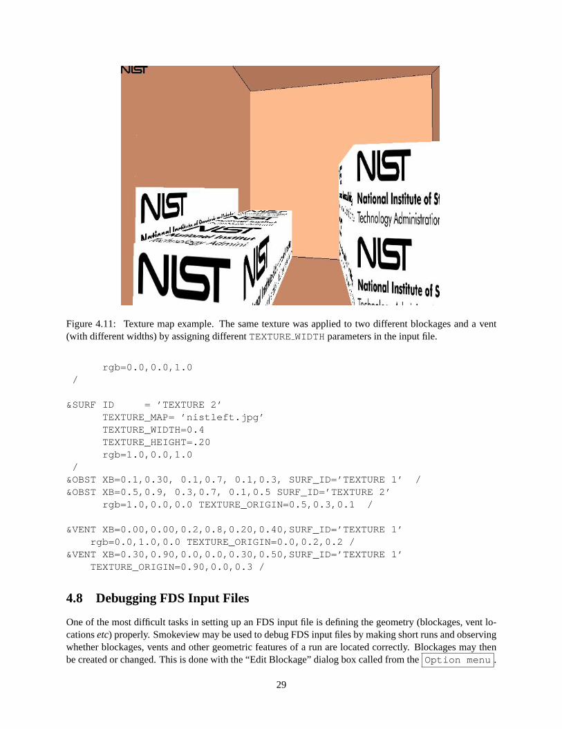
Figure 4.11: Texture map example. The same texture was applied to two different blockages and a vent(with different widths) by assigning differentTEXTUREWIDTHparameters in the input file.
rgb=0.0,0.0,1.0/
&SURF ID = ’TEXTURE 2’TEXTURE_MAP= ’nistleft.jpg’TEXTURE_WIDTH=0.4TEXTURE_HEIGHT=.20rgb=1.0,0.0,1.0
/&OBST XB=0.1,0.30, 0.1,0.7, 0.1,0.3, SURF_ID=’TEXTURE 1’ /&OBST XB=0.5,0.9, 0.3,0.7, 0.1,0.5 SURF_ID=’TEXTURE 2’
rgb=1.0,0.0,0.0 TEXTURE_ORIGIN=0.5,0.3,0.1 /
&VENT XB=0.00,0.00,0.2,0.8,0.20,0.40,SURF_ID=’TEXTURE 1’rgb=0.0,1.0,0.0 TEXTURE_ORIGIN=0.0,0.2,0.2 /
&VENT XB=0.30,0.90,0.0,0.0,0.30,0.50,SURF_ID=’TEXTURE 1’TEXTURE_ORIGIN=0.90,0.0,0.3 /
4.8 Debugging FDS Input Files
One of the most difficult tasks in setting up an FDS input file is defining the geometry (blockages, vent lo-cationsetc) properly. Smokeview may be used to debug FDS input files by making short runs and observingwhether blockages, vents and other geometric features of a run are located correctly. Blockages may thenbe created or changed. This is done with the “Edit Blockage” dialog box called from theOption menu .
29
The following is a general procedure for identifying problems in FDS input files. Assume that the FDSinput data file is namedtestcase1.data .
1. Set the stop time to 0.0 usingTWFIN=0.0 on the&TIME line. This causes FDS to read the input fileand create a.smv file without performing lengthy startup calculations.
2. After the input file has been modified, run the FDS model (for details see the FDS User’s Guide[1])
FDS creates a file namedtestcase1.smv containing information that Smokeview uses to visual-ize data.
3. To visualize the input file, opentestcase1.smv with Smokeview by either typingsmokeviewtestcase1 at a command shell prompt or if on the PC by double-clicking the filetestcase1.smv .
4. Make corrections if necessary. Use theCOLORor RGBoption2 of theOBSTkeyword to more easilyidentify blockages to be edited. For example, to change a blockage’s color to red use:
&OBST XB=0.0,1.0,0.0,1.0,0.0,1.0 COLOR=’RED’ /
or
&OBST XB=0.0,1.0,0.0,1.0,0.0,1.0 RGB=1.0,0.0,0.0 /
Save testcase1.data file and go back to step 2.
5. If corrections are unnecessary, then change theTWFINkeyword back to the desired final simulationtime, remove any unnecessary FDSCOLORkeywords and run the case.
Examining and/or Editing Blockages Blockages may be examined or changed by selectingDialogs/Edit Geometrywhich opens up the dialog box illustrated in Figure 4.12. Text edit boxes allow one to define comments (anytext to the right of the closing “/” on an &OBST line and pull down menus for linking surfaces (&SURFlines) to obstructions. The surface choices are obtained from the input file or the database file if one isspecified in the input file.
Note, the blockage editor does not work when clipping planes are active.The user may associate one, three or six surfaces with an obstruction. If the “3 wall ” radio button
is selected then materials for the ceiling (upper surface), walls (vertical surfaces) and floor (lower surface)may be specified. The “color ” check box allows the inputted or default color (manilla) to be displayed onblockage surfaces.
Associating unique colors with each surface allows the user to quickly determine whether blockages aredefined with the proper surfaces. One can then verify that these modelling elements have been defined andpositioned as intended.
The blockage editor works on one mesh at a time. For multi-mesh cases, use the Mesh list-box to selectthe desired mesh or simply click on a blockage in the mesh to switch to that mesh. The pull-down menu isnecessary for meshes without blockages.
Position coordinates entered into the text boxes are “snapped” to the nearest grid line. Materials appear-ing under “Surface Type ” come from those materials defined in either the input data file or the databasefile. Either one, three or six wall properties can be entered by selecting the appropriate radio button.
2The FDSCOLORkeyword may have values:RED, BLUE, GREEN, MAGENTA, CYAN, YELLOW, WHITEor BLACK. TheRGBkeyword uses three floating point inputs ranging from 0.0 to 1.0 to specify the red, green and blue components of color.COLORreplacesBLOCKCOLORandVENTCOLOR.
30
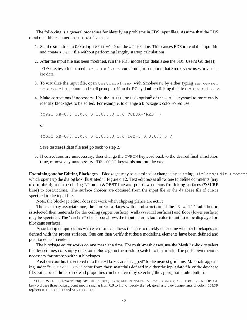
Figure 4.12: Blockage Edit Dialog Box. Click on ‘New’ to create a new blockage or click on an existingblockage in the Smokeview scene to change its size or location. Change the size or location by enteringblockage bounds directly or clicking an ‘arrow’ and/or direction buttons. Note, the blockage editor does notwork when clipping planes are active.
4.9 Making Movies
A movie can be made of a Smokeview animation by converting the visualized scene into a series of PNGor JPEG files, one file for each time step and then combining the individual images together into one moviefile. More specifically:
1. Set up Smokeview by orienting the scene and loading the desired data files.
2. Select theOptions/Render menu and pick the desired frame skip value. The more frames youinclude in the animation, the smoother it will look. Of course more frames result in larger file sizes.Choose fewer frames if the movie is to appear on a web site.
3. Use a program such as the Antechinus Media Editor available at http://www.c-point.com to assemblethe JPEGS or PNGS rendered in the previous step into a movie file.
The default Smokeview image size is 640×480 . This size is fine if the movie is to appear in a presen-tation located on a local hard disk. If the movie is to be placed on a web site then care needs to be takento insure that the generated movie file is a reasonable size. Two suggestions are to reduce the image size to320×240 or smaller by modifying theWINDOWWIDTHandWINDOWHEIGHTsmokeview.ini keywords andto reduce the number of frames to 300 or less by skipping intermediate framesvia the Options/Rendermenu.
Sometimes when copying or “capturing” a Smokeview scene it is desirable, or even necessary, to havea margin around the scene. This is because the capturing system does not include the entire scene butitself captures an indented portion of the scene. To indent the scene, either press the “h” key or select theOption >Viewpoint >Offset Window menu item. The default indentation is 45 pixels. This may
be changed by adding/editing the WINDOWOFFSET keyword in the smokeview.ini file.
31
4.10 Annotating the Scene
Smokeview rendered JPEG or PNG image files may be annotated with any package that edits these typesof files. Tick marks and label annotation can be placed within the 3D scene and moved around as the sceneis moved. This would be difficult to duplicate with an external image editor. In addition, axis labels aredisplayed, if desired, by selectingShow/Hide > Labels > Axis labels .
The current release of FDS places tick marks and labels documenting the scene dimensions. To replaceor customize these annotations add theTICK keyword to a .smv file using the following format:
TICKSxb yb zb xe ye ze nticksticklength tickdir r g b tickwidth
wherexb , yb , andzb are the x, y and z coordinates of the first tick;xe , ye andze are the x, y and zcoordinates of the last tick andnticks is the number of ticks. The coordinate dimensions are in physicalunits, the same units used to set up the FDS geometry. The parameterticklength specifies the lengh ofthe tick in physical units. The parametertickdir specifies the tick direction. For example 1(-1) placesticks in the positive(negative) x direction. Similarly, 2(-2) and 3(-3) place ticks in the positive(negative) yand positive(negative) z directions.
The color parametersr , g andb are the red, green and blue components of the tick color each rangingfrom 0.0 to 1.0. The foreground color (white by default) may be set by setting any or all of ther , g andb components to a negative number. Thetickwidth parameter specifies tick width in pixels. Fractionalwidths may be specified.
TheLABEL keyword allows a text string to be added within a Smokeview scene. The label color andstart and stop appearance time may also be specified. The format is given by
LABELSx y z r g b tstart tstoplabel
where (x, y, z ) is the label location in cartesian coordinates andr, g, b are the red, green and bluecolor components ranging from 0.0 to 1.0. Again, if a negative value is specified then the foreground colorwill be used instead (white is the default). The parameters,tstart andtstop indicate the time intervalwhen the label is visible. The text string is specified on the next line (label ).
Figure 4.13 shows how theLABEL andTICKS keywords can be used together to create a “ruler” withmajor and minor tick marks. These ticks and labels were created using:
TICKS0.0 0.0 0.0 8.0 0.0 0.0 50.5 -2.0 -1. -1.0 -1.0 4.0TICKS1.0 0.0 0.0 9.0 0.0 0.0 50.25 -2.0 -1. -1.0 -1.0 4.0TICKS0.0 0.0 0.0 0.0 0.0 2.0 30.5 -1.0 -1. -1.0 -1.0 4.0TICKS0.0 0.0 0.0 0.0 4.0 0.0 50.5 -1.0 -1. -1.0 -1.0 4.0LABEL0.0 -0.6 0.0 -1.0 0.0 0.0 0.0 20.0
32
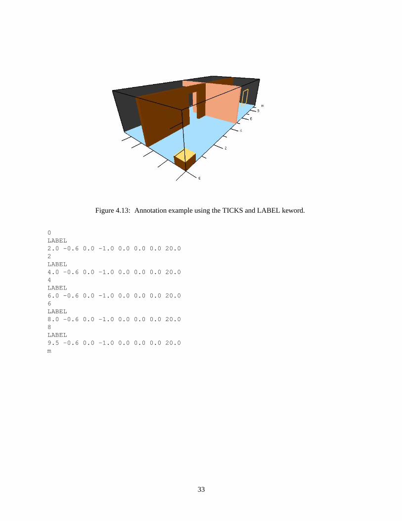
Figure 4.13: Annotation example using the TICKS and LABEL keword.
0LABEL2.0 -0.6 0.0 -1.0 0.0 0.0 0.0 20.02LABEL4.0 -0.6 0.0 -1.0 0.0 0.0 0.0 20.04LABEL6.0 -0.6 0.0 -1.0 0.0 0.0 0.0 20.06LABEL8.0 -0.6 0.0 -1.0 0.0 0.0 0.0 20.08LABEL9.5 -0.6 0.0 -1.0 0.0 0.0 0.0 20.0m
33

34
Chapter 5
Summary
Often fire modeling is looked upon with skepticism because of the perception that eye-catching imagesshroud the underlying physics. However, if the visualization is done well, it can be used to assess the qualityof the simulation technique. The user of FDS chooses a numerical grid on which to discretize the governingequations. The more grid cells, the better but more time-consuming the simulation. The payoff for investingin faster computers and running bigger calculations is the proportional gain in realism manifested by theimages. There is no better way to demonstrate the quality of the calculation than by showing the realisticbehavior of the fire.
Up to now, most visualization techniques have provided useful ways of analyzing the output of a calcu-lation, like contour and streamline plots, without much concern for realism. A rainbow-colored contour mapslicing down through the middle of a room is fine for researchers, but for those who are only accustomed tolooking at real smoke-filled rooms, it may not have as much meaning. Good visualization needs to provideas much information as the rainbow contour map but in a way that speaks to modelers and non-modelersalike. A good example is smoke visibility. Unlike temperature or species concentration, smoke visibility isnot a local quantity but rather depends on the viewpoint of the eye and the depth of field. Advanced simula-tors and games create the illusion of smoke or fog in ways that are not unlike the techniques employed byfire models to handle thermal radiation. The visualization of smoke and fire by Smokeview is an exampleof the graphics hardware and software actually computing results rather than just drawing pretty pictures. Acommon concern in the design of smoke control systems is whether or not building occupants will be able tosee exit signs at various stages of a fire. FDS can predict the amount of soot is located at any given point, butthat doesn’t answer the question. The harder task is to compute on the fly within the visualization programwhat the occupant would see and not see. In this sense, Smokeview is not merely a “post-processor,” butrather an integral part of the analysis.
35

36
Bibliography
[1] K.B. McGrattan and G.P. Forney. Fire Dynamics Simulator (Version 4), User’s Guide. NIST SpecialPublication 1019, National Institute of Standards and Technology, Gaithersburg, Maryland, July 2004.
[2] K.B. McGrattan (editor). Fire Dynamics Simulator (Version 4), Technical Reference Guide. NISTSpecial Publication 1018, National Institute of Standards and Technology, Gaithersburg, Maryland,July 2004.
[3] G. P. Forney and K. B. McGrattan. User’s Guide for Smokeview Version 3.1: A Tool for VisualizingFire Dynamics Simulation Data. NISTIR 6980, National Institute of Standards and Technology, April2003.
[4] D. Madrzykowski and R.L. Vettori. Simulation of the Dynmaics of the Fire at 3146 Cherry Road NE,Washington, DC May 30, 1999. Technical Report NISTIR 6510, Gaithersburg, Maryland, April 2000.URL: http://fire.nist.gov/6510.
[5] D. Madrzykowski, G.P. Forney, and W.D. Walton. Simulation of the Dynamics of a Fire in a Two-StoryDuplex, Iowa, December 22, 1999. Technical Report NISTIR 6854, Gaithersburg, Maryland, January2002. URL: http://www.fire.nist.gov/bfrlpubs/duplex/duplex.htm.
[6] R.L. Vettori, D. Madrzykowski, and W.D. Walton. Simulation of the Dynamics of a Fire in a One-StoryRestaurant – Texas, February 14, 2000. Technical Report NISTIR 6923, Gaithersburg, Maryland,October 2002.
[7] R.G. Rehm, W.M. Pitts, Baum H.R., Evans D.D., K. Prasad, K.B. McGrattan, and G.P. Forney. InitialModel for Fires in the World Trade Center Towers. Technical Report NISTIR 6879, Gaithersburg,Maryland, May 2002.
[8] Mason Woo, Jackie Neider, Tom Davis, and Dave Shreiner.OpenGL Programming Guide. Addison-Wesley, Reading, Massachussets, 3 edition, 1999.
[9] Mark J. Kilgard.OpenGL Programming for the X Window System. Addison-Wesley Developers Press,Reading, Massachussets, 1996.
[10] Thomas Boutell.CGI Programming in C & Perl. Addison-Wesley Publishing Co., Reading, Mas-sachussets, 1996.
[11] Thomas Boutell. GD version 2.0.7, http://www.boutell.com/gd/, November 2002.
[12] Guy Eric Schalnat, Andreas Dilger, and Glenn Randers-Pehrson. libpng version 1.2.5,http://www.libpng.org/pub/png/, November 2002.
[13] jpeg version 6b, http://www.ijg.org/.
37

[14] Jean loup Gailly and Mark Adler. zlib version 1.1.4, http://www.gzip.org/zlib/, November 2002.
[15] Paul Rademacher. GLUI version 2.1, http://www.cs.unc.edu/ rademach/glui/.
[16] Tomas Akenine-Moller.Real-Time Rendering. A K Peters, Ltd., 2002.
[17] Pamela P. Walatka and Pieter G. Buning. PLOT3D User’s Manual, version 3.5. NASA TechnicalMemorandum 101067, NASA, 1989.
38
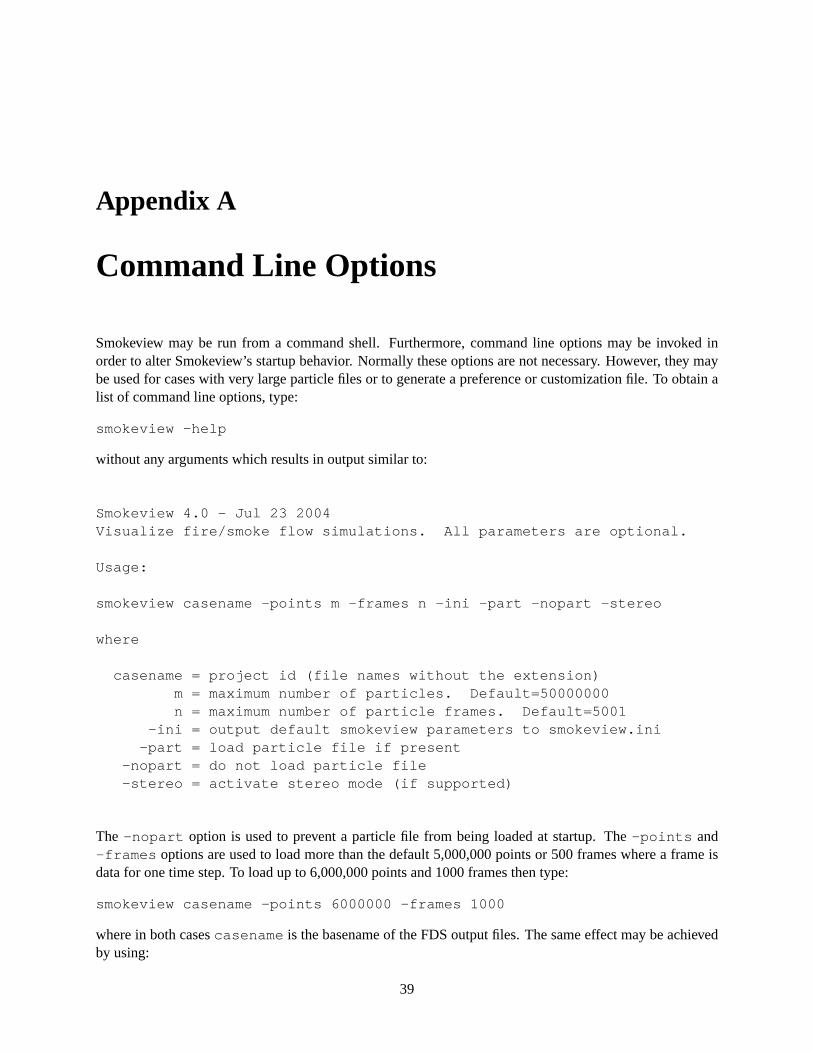
Appendix A
Command Line Options
Smokeview may be run from a command shell. Furthermore, command line options may be invoked inorder to alter Smokeview’s startup behavior. Normally these options are not necessary. However, they maybe used for cases with very large particle files or to generate a preference or customization file. To obtain alist of command line options, type:
smokeview -help
without any arguments which results in output similar to:
Smokeview 4.0 - Jul 23 2004Visualize fire/smoke flow simulations. All parameters are optional.
Usage:
smokeview casename -points m -frames n -ini -part -nopart -stereo
where
casename = project id (file names without the extension)m = maximum number of particles. Default=50000000n = maximum number of particle frames. Default=5001
-ini = output default smokeview parameters to smokeview.ini-part = load particle file if present
-nopart = do not load particle file-stereo = activate stereo mode (if supported)
The -nopart option is used to prevent a particle file from being loaded at startup. The-points and-frames options are used to load more than the default 5,000,000 points or 500 frames where a frame isdata for one time step. To load up to 6,000,000 points and 1000 frames then type:
smokeview casename -points 6000000 -frames 1000
where in both casescasename is the basename of the FDS output files. The same effect may be achievedby using:
39

MAXPOINTS6000000MAXFRAMES1000
in the smokeview.ini or casename.ini file. This file may be created with the-ini option andcontains many other customizable Smokeview parameters. The-benchmark option is used to measurethe performance of Smokeview. The-benchmark option causes Smokeview to produce precise timingsby outputting frame rates based upon one cycle through the timing loop rather than using moving averages.The-stereo option may used to access stereo hardware (often called quad buffering) if it is available.
40
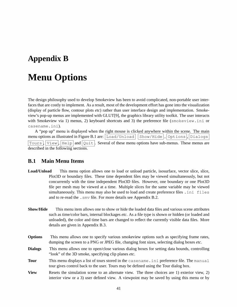
Appendix B
Menu Options
The design philosophy used to develop Smokeview has been to avoid complicated, non-portable user inter-faces that are costly to implement. As a result, most of the development effort has gone into the visualization(display of particle flow, contour plotsetc) rather than user interface design and implementation. Smoke-view’s pop-up menus are implemented with GLUT[9], the graphics library utility toolkit. The user interactswith Smokeview via 1) menus, 2) keyboard shortcuts and 3) the preference file (smokeview.ini orcasename.ini ).
A “pop up” menu is displayed when the right mouse is clicked anywhere within the scene. The mainmenu options as illustrated in Figure B.1 are:Load/Unload Show/Hide , Options , Dialogs
Tours , View , Help and Quit . Several of these menu options have sub-menus. These menus aredescribed in the following sections.
B.1 Main Menu Items
Load/Unload This menu option allows one to load or unload particle, isosurface, vector slice, slice,Plot3D or boundary files. These time dependent files may be viewed simultaneously, but notconcurrently with the time independent Plot3D files. However, one boundary or one Plot3Dfile per mesh may be viewed at a time. Multiple slices for the same variable may be viewedsimultaneously. This menu may also be used to load and create preference files.ini filesand to re-read the.smv file. For more details see Appendix B.2.
Show/Hide This menu item allows one to show or hide the loaded data files and various scene attributessuch as time/color bars, internal blockagesetc. As a file type is shown or hidden (or loaded andunloaded), the color and time bars are changed to reflect the currently visible data files. Moredetails are given in Appendix B.3.
Options This menu allows one to specify various smokeview options such as specifying frame rates,dumping the screen to a PNG or JPEG file, changing font sizes, selecting dialog boxesetc.
Dialogs This menu allows one to open/close various dialog boxes for setting data bounds, controlling“look” of the 3D smoke, specifying clip planesetc.
Tour This menu displays a list of tours stored in thecasename.ini preference file. Themanualtour gives control back to the user. Tours may be defined using the Tour dialog box.
View Resets the simulation scene to an alternate view. The three choices are 1) exterior view, 2)interior view or a 3) user defined view. A viewpoint may be saved by using this menu or by
41
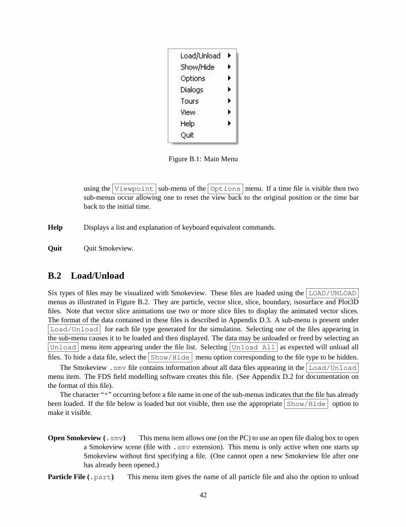
Figure B.1: Main Menu
using the Viewpoint sub-menu of theOptions menu. If a time file is visible then twosub-menus occur allowing one to reset the view back to the original position or the time barback to the initial time.
Help Displays a list and explanation of keyboard equivalent commands.
Quit Quit Smokeview.
B.2 Load/Unload
Six types of files may be visualized with Smokeview. These files are loaded using theLOAD/UNLOADmenus as illustrated in Figure B.2. They are particle, vector slice, slice, boundary, isosurface and Plot3Dfiles. Note that vector slice animations use two or more slice files to display the animated vector slices.The format of the data contained in these files is described in Appendix D.3. A sub-menu is present underLoad/Unload for each file type generated for the simulation. Selecting one of the files appearing in
the sub-menu causes it to be loaded and then displayed. The data may be unloaded or freed by selecting anUnload menu item appearing under the file list. SelectingUnload All as expected will unload all
files. To hide a data file, select theShow/Hide menu option corresponding to the file type to be hidden.
The Smokeview.smv file contains information about all data files appearing in theLoad/Unloadmenu item. The FDS field modelling software creates this file. (See Appendix D.2 for documentation onthe format of this file).
The character “* ” occurring before a file name in one of the sub-menus indicates that the file has alreadybeen loaded. If the file below is loaded but not visible, then use the appropriateShow/Hide option tomake it visible.
Open Smokeview (.smv ) This menu item allows one (on the PC) to use an open file dialog box to opena Smokeview scene (file with.smv extension). This menu is only active when one starts upSmokeview without first specifying a file. (One cannot open a new Smokeview file after onehas already been opened.)
Particle File (.part ) This menu item gives the name of all particle file and also the option to unload
42
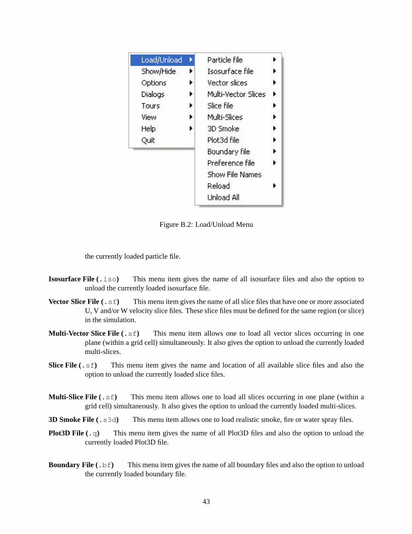
Figure B.2: Load/Unload Menu
the currently loaded particle file.
Isosurface File (.iso ) This menu item gives the name of all isosurface files and also the option tounload the currently loaded isosurface file.
Vector Slice File (.sf ) This menu item gives the name of all slice files that have one or more associatedU, V and/or W velocity slice files. These slice files must be defined for the same region (or slice)in the simulation.
Multi-Vector Slice File ( .sf ) This menu item allows one to load all vector slices occurring in oneplane (within a grid cell) simultaneously. It also gives the option to unload the currently loadedmulti-slices.
Slice File (.sf ) This menu item gives the name and location of all available slice files and also theoption to unload the currently loaded slice files.
Multi-Slice File ( .sf ) This menu item allows one to load all slices occurring in one plane (within agrid cell) simultaneously. It also gives the option to unload the currently loaded multi-slices.
3D Smoke File (.s3d ) This menu item allows one to load realistic smoke, fire or water spray files.
Plot3D File (.q ) This menu item gives the name of all Plot3D files and also the option to unload thecurrently loaded Plot3D file.
Boundary File (.bf ) This menu item gives the name of all boundary files and also the option to unloadthe currently loaded boundary file.
43
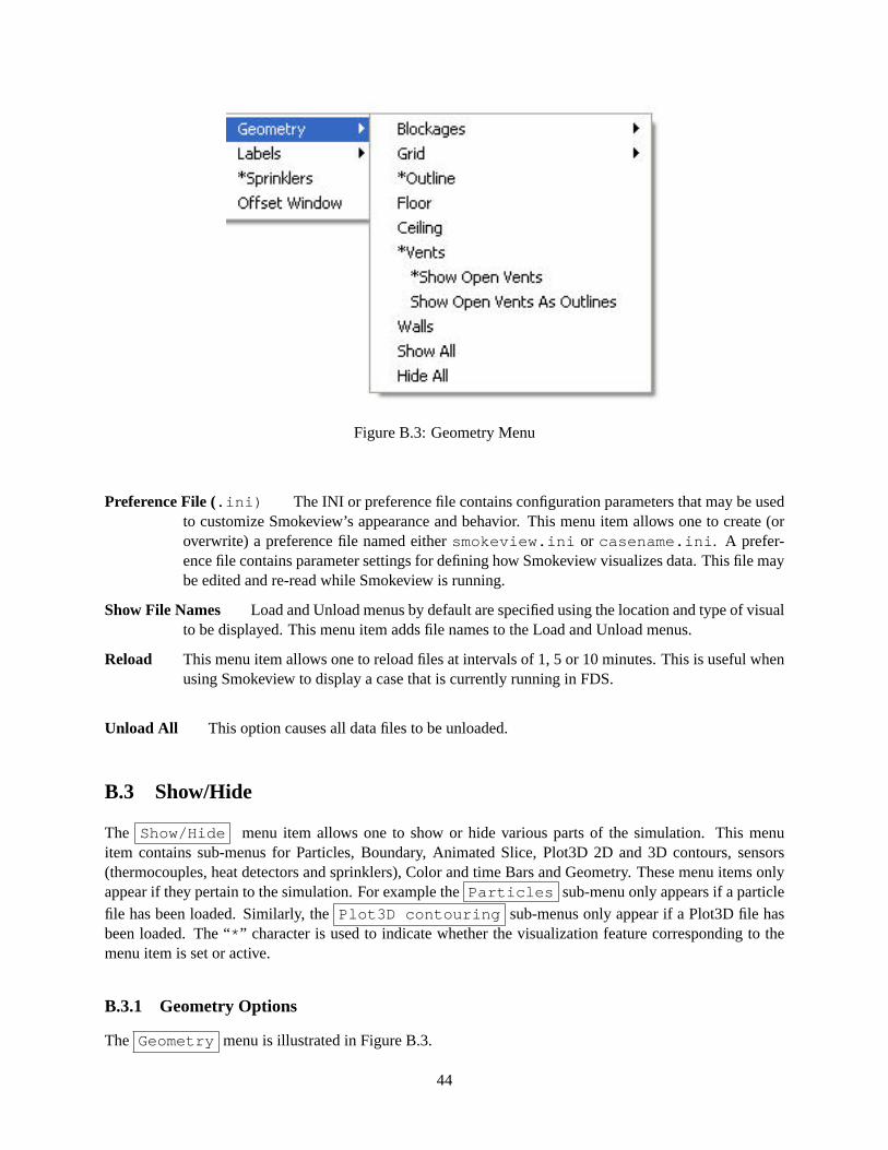
Figure B.3: Geometry Menu
Preference File (.ini) The INI or preference file contains configuration parameters that may be usedto customize Smokeview’s appearance and behavior. This menu item allows one to create (oroverwrite) a preference file named eithersmokeview.ini or casename.ini . A prefer-ence file contains parameter settings for defining how Smokeview visualizes data. This file maybe edited and re-read while Smokeview is running.
Show File Names Load and Unload menus by default are specified using the location and type of visualto be displayed. This menu item adds file names to the Load and Unload menus.
Reload This menu item allows one to reload files at intervals of 1, 5 or 10 minutes. This is useful whenusing Smokeview to display a case that is currently running in FDS.
Unload All This option causes all data files to be unloaded.
B.3 Show/Hide
The Show/Hide menu item allows one to show or hide various parts of the simulation. This menuitem contains sub-menus for Particles, Boundary, Animated Slice, Plot3D 2D and 3D contours, sensors(thermocouples, heat detectors and sprinklers), Color and time Bars and Geometry. These menu items onlyappear if they pertain to the simulation. For example theParticles sub-menu only appears if a particlefile has been loaded. Similarly, thePlot3D contouring sub-menus only appear if a Plot3D file hasbeen loaded. The “* ” character is used to indicate whether the visualization feature corresponding to themenu item is set or active.
B.3.1 Geometry Options
The Geometry menu is illustrated in Figure B.3.
44

Blockages Blockage sub-menus are divided into two groups. The first group allows the user to changehow blockage appear (Defined in Input File , Normal , Outline , Hidden ).
The second group allows the user to change where blockages are located (actual or re-quested). TheActual sub-menu positions blockages as computed by FDS (along grid lines).The Requested sub-menu positions blockages at locations as specified in the input file.If the dx2dxf conversion program was used to convert a Cad drawing to input compatiblewith FDS and Smokeview then a third menu option appears,Cad . This option displays theSmokeview scene in a form similar to the original Cad drawing.
Grid This option allows one to visualize the grid used to perform the numerical calculations. Oneselectsxy plane , xz plane or yz plane to visualize a single plane orShow All ,
Hide All to show or hide all grids. (Keyboard shortcut:g)
Outline Show or hide the outline that frames the simulation scene.
Floor Show or hide the floor.
Ceiling Show or hide the ceiling.
Vents Show or hide the vents.
Walls Show or hide the walls.
Show All Show all geometric features described above.
Hide All Hide all geometric features described above.
B.3.2 Animated Surface
This menu allows one to control the way isosurfaces are displayed. An isosurface is represented in Smoke-view as a collection of triangles. Each triangle consists of three edges and three vertices.
Solid Display the isosurface by shading the triangles.
Outline Display the isosurface by only showing the triangle edges.
Points Display the isosurface by only showing the triangle vertices.
“quantity” levels Display the desired isosurface level (when more than one isosurface is stored in anisosurface file).
Smooth Display the isosurface using smoothed vertex normals.
B.3.3 Particles
Smoke (tracer) Toggle the visibility of the particles. If water/sprinkler droplets are present in the parti-cle file then sub-menus exist for both smoke and water to allow one to show or hide smoke andwater droplets independently.
Sprinkler Toggle the visibility of sprinkler (water droplets).
B.3.4 Boundary
Exterior Show or hide all data contained in a boundary (.bf ) file pertaining to the exterior walls.
45
Interior Show or hide all data contained in a boundary (.bf ) file pertaining to interior blockages.
Front, Back, Left, Right, Up, Down Toggle the visibility of whatever exterior boundary surface is se-lected. Note an exterior boundary menu option only appears if its data is present in the boundaryfile.
B.3.5 Animated Vector Slice
Toggle the visibility of the animated vector slice file.
B.3.6 Animated Slice
Toggle the visibility of the animated slice file.
B.3.7 Plot3D
2D Contours
Solution Variables A Plot3D data file contains five solution variables. If one or more of the velocitycomponents denotedu, v and w are present in the Plot3D file then speed, calculated using√
u2 +v2 +w2, appears in the menu. Any velocity components missing from the Plot3D fileare set to 0.0 when calculating speed. This menu item allows one to select the Plot3D solutionvariable to be visualized. (Keyboard shortcut:p)
xy, xz, yz planes These three menu items, appearing beneath theSolution Variables menuitem, allow one to select which plane (xy, xz or yz) is displayed. (Applicable keyboard short-cuts: space bar, -, left/right cursor, up/down cursor, page up/down,1...9 )
Flow vectors Toggle visibility of flow vectors. The magnitude and direction of the vectors are de-termined by the U, V and W components of velocity. The vector color is determined by thesolution variable selected. (Applicable keyboard shortcuts:a, s, v )
Continuous Display contours as smooth continuous shades or as stepped constant shades. (Keyboardshortcut:c )
Show All Show all three (xy, xz and yz) Plot3D planes at once.
Hide All Hide all three Plot3D planes.
Plot3D 3D Contours
Solution Variables Same as for 2D contours. This menu item allows one to select the solution variableused to generate the 3D or iso-contour to be displayed.
Solution Value Select the 3D contour level to display. The axis label shown in red corresponds to the3D contour level displayed.
Block Size To increase the drawing speed, adjacent grid cells may be combined when viewing 3D con-tours. Selecting 1 will result in highly resolved contours but may take longer to draw. Selecting5 will have the opposite effect.
Hide Hide the 3D contour.
46
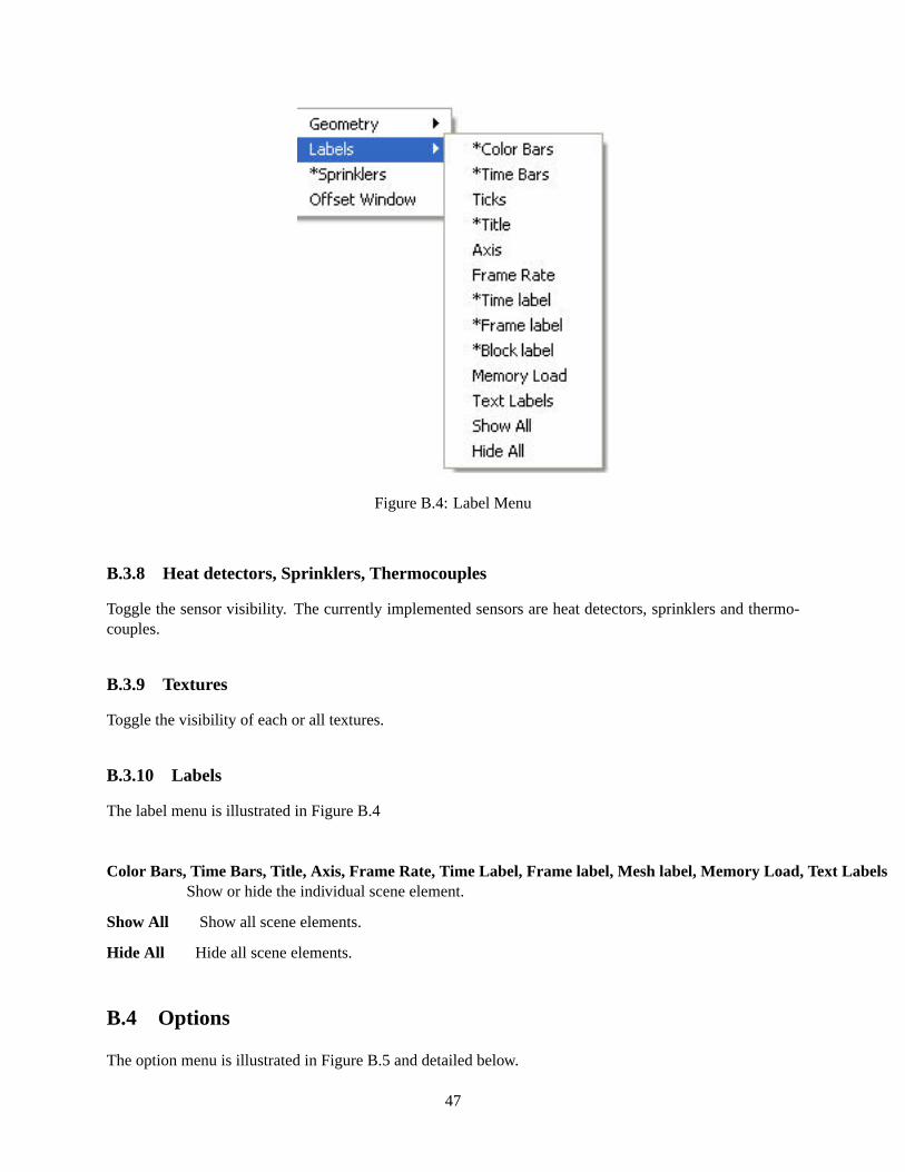
Figure B.4: Label Menu
B.3.8 Heat detectors, Sprinklers, Thermocouples
Toggle the sensor visibility. The currently implemented sensors are heat detectors, sprinklers and thermo-couples.
B.3.9 Textures
Toggle the visibility of each or all textures.
B.3.10 Labels
The label menu is illustrated in Figure B.4
Color Bars, Time Bars, Title, Axis, Frame Rate, Time Label, Frame label, Mesh label, Memory Load, Text LabelsShow or hide the individual scene element.
Show All Show all scene elements.
Hide All Hide all scene elements.
B.4 Options
The option menu is illustrated in Figure B.5 and detailed below.
47
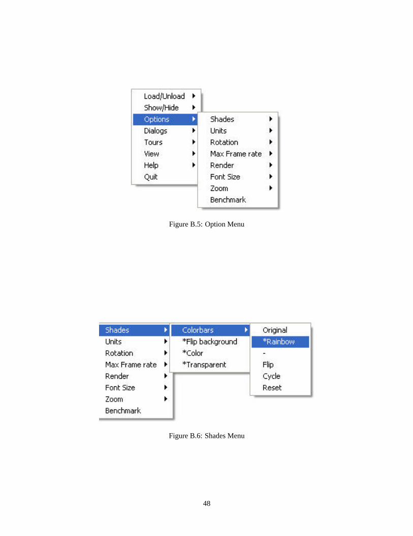
Figure B.5: Option Menu
Figure B.6: Shades Menu
48
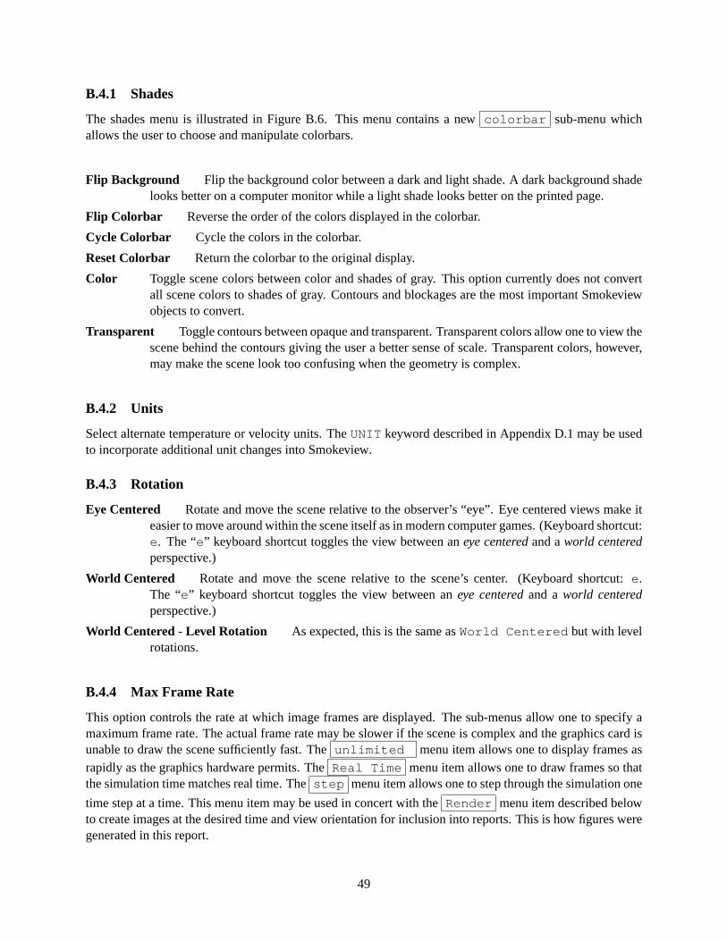
B.4.1 Shades
The shades menu is illustrated in Figure B.6. This menu contains a newcolorbar sub-menu whichallows the user to choose and manipulate colorbars.
Flip Background Flip the background color between a dark and light shade. A dark background shadelooks better on a computer monitor while a light shade looks better on the printed page.
Flip Colorbar Reverse the order of the colors displayed in the colorbar.
Cycle Colorbar Cycle the colors in the colorbar.
Reset Colorbar Return the colorbar to the original display.
Color Toggle scene colors between color and shades of gray. This option currently does not convertall scene colors to shades of gray. Contours and blockages are the most important Smokeviewobjects to convert.
Transparent Toggle contours between opaque and transparent. Transparent colors allow one to view thescene behind the contours giving the user a better sense of scale. Transparent colors, however,may make the scene look too confusing when the geometry is complex.
B.4.2 Units
Select alternate temperature or velocity units. TheUNIT keyword described in Appendix D.1 may be usedto incorporate additional unit changes into Smokeview.
B.4.3 Rotation
Eye Centered Rotate and move the scene relative to the observer’s “eye”. Eye centered views make iteasier to move around within the scene itself as in modern computer games. (Keyboard shortcut:e. The “e” keyboard shortcut toggles the view between aneye centeredand aworld centeredperspective.)
World Centered Rotate and move the scene relative to the scene’s center. (Keyboard shortcut:e.The “e” keyboard shortcut toggles the view between aneye centeredand aworld centeredperspective.)
World Centered - Level Rotation As expected, this is the same asWorld Centered but with levelrotations.
B.4.4 Max Frame Rate
This option controls the rate at which image frames are displayed. The sub-menus allow one to specify amaximum frame rate. The actual frame rate may be slower if the scene is complex and the graphics card isunable to draw the scene sufficiently fast. Theunlimited menu item allows one to display frames asrapidly as the graphics hardware permits. TheReal Time menu item allows one to draw frames so thatthe simulation time matches real time. Thestep menu item allows one to step through the simulation one
time step at a time. This menu item may be used in concert with theRender menu item described belowto create images at the desired time and view orientation for inclusion into reports. This is how figures weregenerated in this report.
49
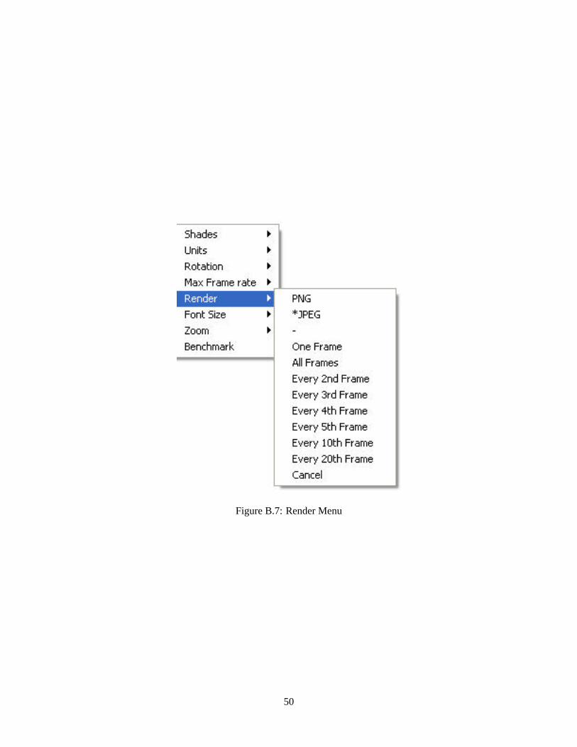
Figure B.7: Render Menu
50
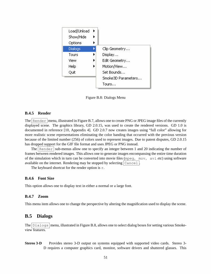
Figure B.8: Dialogs Menu
B.4.5 Render
The Render menu, illustrated in Figure B.7, allows one to create PNG or JPEG image files of the currentlydisplayed scene. The graphics library, GD 2.0.15, was used to create the rendered versions. GD 1.0 isdocumented in reference [10, Appendix 4]. GD 2.0.7 now creates images using “full color” allowing formore realistic scene representations eliminating the color banding that occurred with the previous versionbecause of the limited number (256) of colors used to represent images. Due to patent disputes, GD 2.0.15has dropped support for the GIF file format and uses JPEG or PNG instead.
The Render sub-menus allow one to specify an integer between 1 and 20 indicating the number offrames between rendered images. This allows one to generate images encompassing the entire time durationof the simulation which in turn can be converted into movie files (mpeg, mov, avi etc) using softwareavailable on the internet. Rendering may be stopped by selectingCancel .
The keyboard shortcut for the render option isr .
B.4.6 Font Size
This option allows one to display text in either a normal or a large font.
B.4.7 Zoom
This menu item allows one to change the perspective by altering the magnification used to display the scene.
B.5 Dialogs
The Dialogs menu, illustrated in Figure B.8, allows one to select dialog boxes for setting various Smoke-view features.
Stereo 3-D Provides stereo 3-D output on systems equipped with supported video cards. Stereo 3-D requires a computer graphics card, monitor, software drivers and shuttered glasses. This
51
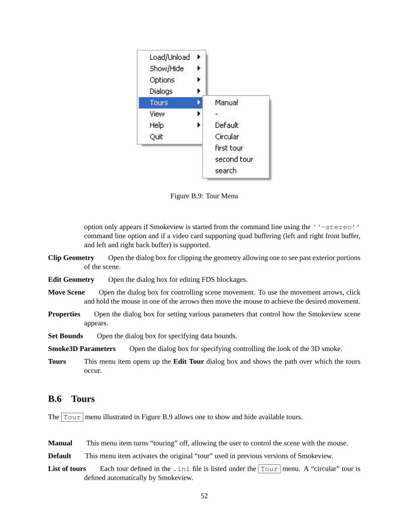
Figure B.9: Tour Menu
option only appears if Smokeview is started from the command line using the‘‘-stereo’’command line option and if a video card supporting quad buffering (left and right front buffer,and left and right back buffer) is supported.
Clip Geometry Open the dialog box for clipping the geometry allowing one to see past exterior portionsof the scene.
Edit Geometry Open the dialog box for editing FDS blockages.
Move Scene Open the dialog box for controlling scene movement. To use the movement arrows, clickand hold the mouse in one of the arrows then move the mouse to achieve the desired movement.
Properties Open the dialog box for setting various parameters that control how the Smokeview sceneappears.
Set Bounds Open the dialog box for specifying data bounds.
Smoke3D Parameters Open the dialog box for specifying controlling the look of the 3D smoke.
Tours This menu item opens up theEdit Tour dialog box and shows the path over which the toursoccur.
B.6 Tours
The Tour menu illustrated in Figure B.9 allows one to show and hide available tours.
Manual This menu item turns “touring” off, allowing the user to control the scene with the mouse.
Default This menu item activates the original “tour” used in previous versions of Smokeview.
List of tours Each tour defined in the.ini file is listed under theTour menu. A “circular” tour isdefined automatically by Smokeview.
52

Appendix C
Keyboard Shortcuts
Many menu commands have equivalent keyboard shortcuts. These shortcuts are described here and are alsobriefly described under theHelp menu item from within Smokeview itself.
a Alter the arrow size used to display velocity vectors.
b To increase the drawing speed, adjacent grid cells may be combined into coarser pseudo-gridcells when generating and viewing 3D contours. The “b” key is used to increment the numberof grid cells that are combined (between one and five grid cells) when generating 3D contours.Using one grid will result in highly resolved contours but may take longer to draw. Using fivegrid cells will have the opposite effect resulting in coarse contours that can be drawn quickly.
c Toggle the Plot3D 2D contour display between solid banded contours and continuously shadedcontours.
e Toggle how the scene is manipulated between an “eye view” where scene motion is relative tothe observer and a “world view” where the scene motion is relative to the scene center.
g Toggle the grid visibility. When the grid display option is active, the x, y and z keys may beused to show or hide the grid perpendicular to the x, y and z axes respectively.
h Toggle window indentation, for use with window capturing.
i Toggle the visibility of iso-contours (3D surface contours).
k Toggle the visibility of the time bar.
m Switch between blocks in a case that has more than one mesh.
o Reset a time dependent animation to the initial time.
p Show the next variable in the Plot3D data set.
P The cursor keys and the page up/down keys are needed to both move grid and Plot3D planesaround the scene and to move through the scene while in “eye centered” mode. The upper case“P“ key is then used to switch the way these keys are used between grid/Plot3D movementmode and scene movement mode.
q Switch between blockage views. These views are blocks that are aligned on grid lines, blocksas specified by the user (in the .data file) and blocks as generated by a CAD (computer aideddrawing) package.
r Render the current scene as a JPEG or a PNG file which can be viewed in a web browser orinserted into a word processing document.
53
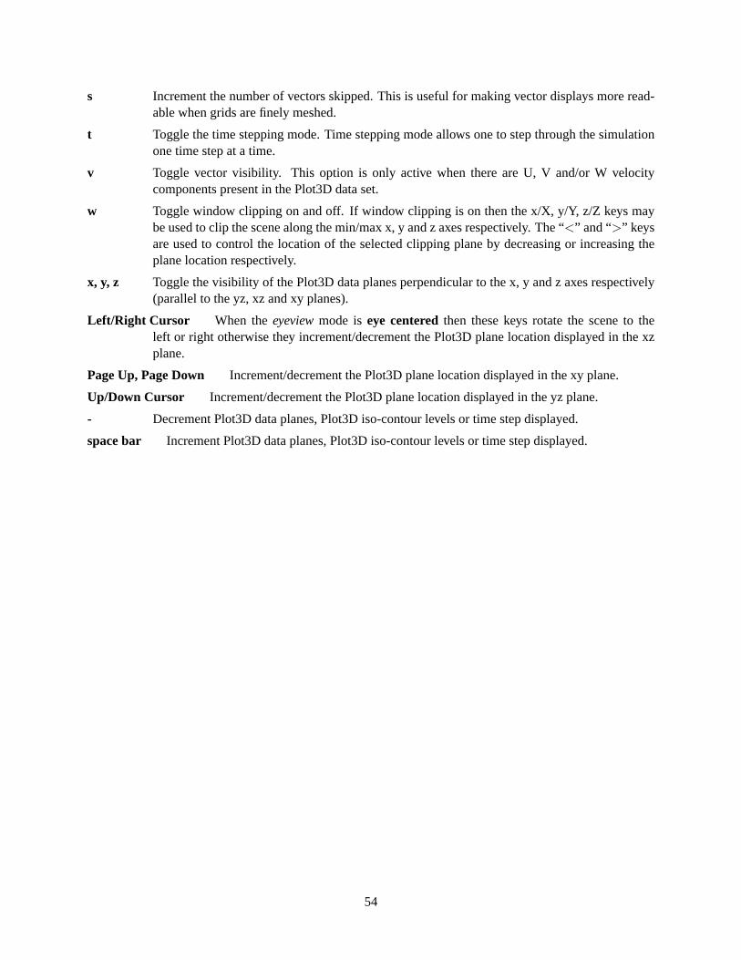
s Increment the number of vectors skipped. This is useful for making vector displays more read-able when grids are finely meshed.
t Toggle the time stepping mode. Time stepping mode allows one to step through the simulationone time step at a time.
v Toggle vector visibility. This option is only active when there are U, V and/or W velocitycomponents present in the Plot3D data set.
w Toggle window clipping on and off. If window clipping is on then the x/X, y/Y, z/Z keys maybe used to clip the scene along the min/max x, y and z axes respectively. The “<” and “>” keysare used to control the location of the selected clipping plane by decreasing or increasing theplane location respectively.
x, y, z Toggle the visibility of the Plot3D data planes perpendicular to the x, y and z axes respectively(parallel to the yz, xz and xy planes).
Left/Right Cursor When theeyeviewmode iseye centeredthen these keys rotate the scene to theleft or right otherwise they increment/decrement the Plot3D plane location displayed in the xzplane.
Page Up, Page Down Increment/decrement the Plot3D plane location displayed in the xy plane.
Up/Down Cursor Increment/decrement the Plot3D plane location displayed in the yz plane.
- Decrement Plot3D data planes, Plot3D iso-contour levels or time step displayed.
space bar Increment Plot3D data planes, Plot3D iso-contour levels or time step displayed.
54
Appendix D
File Formats
D.1 Smokeview Preference File Format (.ini files)
Smokeview uses preference files to set input parameters not settable by using menus or the keyboard and tosave the “state” of a visualization. Smokeview looks for preference files in three locations in the followingorder:
1. a file namedsmokeview.ini in a global directory defined by theSMOKEVIEWINIenvironmentvariable. On the PC, the directoryC: \nist \fds \smokeview.ini is the default location for thispreference file. TheSMOKEVIEWINIenvironment variable may be defined on the PC by adding theline:
set SMOKEVIEWINI=dir
to theC: \autoexec.bat file wheredir is the directory where the global preference file is stored.This step is performed automatically by the Smokeview installation program. This environment vari-able may be defined on a UNIX workstation by adding the line:
setenv SMOKEVIEWINI dir
to a .login or .cshrc start up file again wheredir is the directory containing the global prefer-ence file. Changes to thissmokeview.ini file apply to all cases visualized on the computer unlessoverridden by preference files named or located in directories named in steps 2. and 3.
2. a file namedsmokeview.ini in the directory containing the case being visualized. Changesto this smokeview.ini file apply to all cases in the current directory unless overridden by thecasename.ini file contained in this directory.
3. a file namedcasename.ini in the directory containing the case being visualized where casenameis the name of the case.
Thesmokeview.ini file may be created by typing:
smokeview -ini
from the command line or by selecting theWrite smokeview.ini menu item. Thecasename.inipreference file can be created via the menus or by copying a previously createdsmokeview.ini file.
55
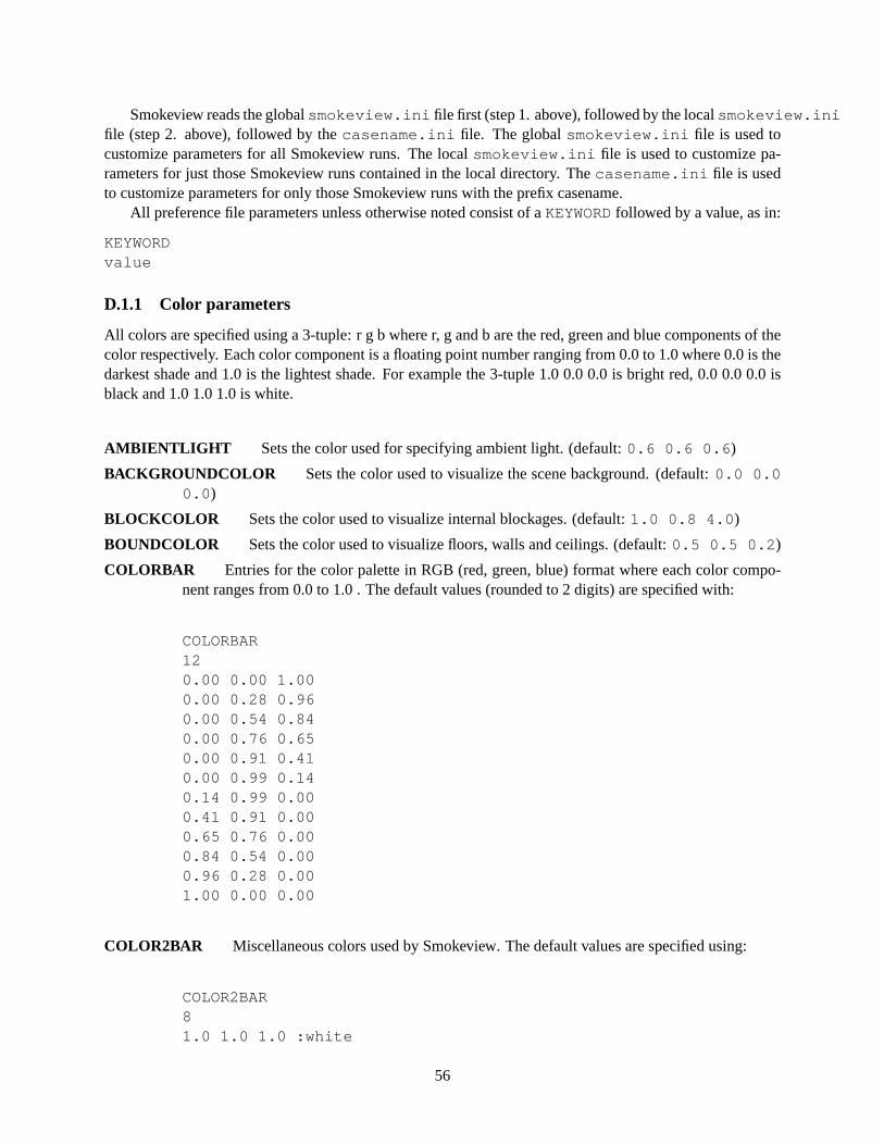
Smokeview reads the globalsmokeview.ini file first (step 1. above), followed by the localsmokeview.inifile (step 2. above), followed by thecasename.ini file. The globalsmokeview.ini file is used tocustomize parameters for all Smokeview runs. The localsmokeview.ini file is used to customize pa-rameters for just those Smokeview runs contained in the local directory. Thecasename.ini file is usedto customize parameters for only those Smokeview runs with the prefix casename.
All preference file parameters unless otherwise noted consist of aKEYWORDfollowed by a value, as in:
KEYWORDvalue
D.1.1 Color parameters
All colors are specified using a 3-tuple: r g b where r, g and b are the red, green and blue components of thecolor respectively. Each color component is a floating point number ranging from 0.0 to 1.0 where 0.0 is thedarkest shade and 1.0 is the lightest shade. For example the 3-tuple 1.0 0.0 0.0 is bright red, 0.0 0.0 0.0 isblack and 1.0 1.0 1.0 is white.
AMBIENTLIGHT Sets the color used for specifying ambient light. (default:0.6 0.6 0.6 )
BACKGROUNDCOLOR Sets the color used to visualize the scene background. (default:0.0 0.00.0 )
BLOCKCOLOR Sets the color used to visualize internal blockages. (default:1.0 0.8 4.0 )
BOUNDCOLOR Sets the color used to visualize floors, walls and ceilings. (default:0.5 0.5 0.2 )
COLORBAR Entries for the color palette in RGB (red, green, blue) format where each color compo-nent ranges from 0.0 to 1.0 . The default values (rounded to 2 digits) are specified with:
COLORBAR120.00 0.00 1.000.00 0.28 0.960.00 0.54 0.840.00 0.76 0.650.00 0.91 0.410.00 0.99 0.140.14 0.99 0.000.41 0.91 0.000.65 0.76 0.000.84 0.54 0.000.96 0.28 0.001.00 0.00 0.00
COLOR2BAR Miscellaneous colors used by Smokeview. The default values are specified using:
COLOR2BAR81.0 1.0 1.0 :white
56
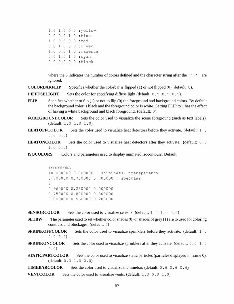
1.0 1.0 0.0 :yellow0.0 0.0 1.0 :blue1.0 0.0 0.0 :red0.0 1.0 0.0 :green1.0 0.0 1.0 :magenta0.0 1.0 1.0 :cyan0.0 0.0 0.0 :black
where the 8 indicates the number of colors defined and the character string after the‘‘:’’ areignored.
COLORBARFLIP Specifies whether the colorbar is flipped (1) or not flipped (0) (default:0).
DIFFUSELIGHT Sets the color for specifying diffuse light (default:0.5 0.5 0.5 ).
FLIP Specifies whether to flip (1) or not to flip (0) the foreground and background colors. By defaultthe background color is black and the foreground color is white. Setting FLIP to 1 has the effectof having a white background and black foreground. (default:0).
FOREGROUNDCOLOR Sets the color used to visualize the scene foreground (such as text labels).(default:1.0 1.0 1.0 )
HEATOFFCOLOR Sets the color used to visualize heat detectors before they activate. (default:1.00.0 0.0 )
HEATONCOLOR Sets the color used to visualize heat detectors after they activate. (default:0.01.0 0.0 )
ISOCOLORS Colors and parameters used to display animated isocontours. Default:
ISOCOLORS10.000000 0.800000 : shininess, transparency0.700000 0.700000 0.700000 : specular30.960000 0.280000 0.0000000.750000 0.800000 0.8000000.000000 0.960000 0.280000
SENSORCOLOR Sets the color used to visualize sensors. (default:1.0 1.0 0.0 )
SETBW The parameter used to set whether color shades (0) or shades of grey (1) are to used for coloringcontours and blockages. (default:0)
SPRINKOFFCOLOR Sets the color used to visualize sprinklers before they activate. (default:1.00.0 0.0 )
SPRINKONCOLOR Sets the color used to visualize sprinklers after they activate. (default:0.0 1.00.0 )
STATICPARTCOLOR Sets the color used to visualize static particles (particles displayed in frame 0).(default:0.0 1.0 0.0 ).
TIMEBARCOLOR Sets the color used to visualize the timebar. (default:0.6 0.6 0.6 )
VENTCOLOR Sets the color used to visualize vents. (default:1.0 0.0 1.0 )
57
D.1.2 Size parameters
The parameters described in this section allow one to customize the size of various Smokeview scene ele-ments.
LINEWIDTH Defines the width of lines1 in pixels. (default: 2.0)
PARTPOINTSIZE Defines the size in pixels of smoke or tracer particles. (default: 1.0)
SENSORABSSIZE Defines the sensor size drawn by smokeview using the same units as used to specifythe grid coordinates. (default: 0.038)
SLICEOFFSET Defines an offset distance2 animated slices are drawn from adjacent solid surfaces.(default: 0.10)
SMOOTHLINES Specifies whether lines should be drawn (1) or not drawn (0) using anti-aliasing(default:1).
SPRINKLERABSSIZE Defines the sprinkler size drawn by smokeview using the same units as usedto specify the grid coordinates. (default: 0.076)
VECTORLENGTH Defines the length of Plot3D vectors. A vector length of 1.0 fills one grid cell.Vector lengths may also be changed from within Smokeview by depressing the “a” key. (de-fault: 4.0)
VECTORPOINTSIZE Defines the size in pixels of the point that is drawn at the end of a Plot3Dvector. (default: 3.0)
VENTLINEWIDTH Defines the width of lines used to draw vents in pixels. (default: 2.0)
VENTOFFSET Defines a distance used to offset vents drawn from adjacent surfaces. (default: 0.10(units of fraction of a grid cell width))
WINDOWHEIGHT Defines the initial window height in pixels. (default: 480)
WINDOWWIDTH Defines the initial window width in pixels. (default: 640)
WINDOWOFFSET Defines a margin offset around the Smokeview scene for use when capturing im-ages to video. (default: 45)
D.1.3 Time, Chop and value bound parameters
This section describes parameters used by Smokeview to 1) modify the time intervals used to load data(keywords beginning with T), 2) eliminate or chop data from being displayed (beginning with C) and3) override the minimum and maximum data values (keywords beginning with V) used to convert data tocolor values. By default, Smokeview reads in data for all time values and does not override minimum andmaximum data values. Each time and data bound keyword (except for VPLOT3D) has the format:
KEYWORDminflag minvalue maxflag maxvalue
whereminflag can be either 0 or 1. If it is 1 then, the subsequent number,minvalue is used by Smoke-view to scale the data otherwise ifminflag is 0 thenminvalue is ignored. The next two parametersmaxflag andmaxvalue are defined similarly. TheV PLOT3Dkeyword contains data bound entries for
1Except lines used to draw vents2distance is relative to the maximum grid cell width
58

each variable in the Plot3D data file. If a Plot3D “speed” variable was constructed by Smokeview then theV PLOT3Dkeyword will contain six entries instead of five.
C PARTICLES Defines the minimum and maximum values used to discard particle data in a visual-ization. To drop particle data below 70◦C and above 200◦C use:
C_PARTICLES 1 70. 1 200.
C PLOT3D Defines the minimum and maximum data values used to drop or chop Plot3D. To causeSmokeview to set the minimum and maximum chop values for the first PLOT3D quantity (usu-ally temperature) to 100 and 300 use:
C_PLOT3D 51 1 100.0 1 300.02 0 1.0 0 0.03 0 1.0 0 0.04 0 1.0 0 0.05 0 1.0 0 0.0
The integer “1” occurring before the “100 ” or “ 300 ” causes Smokeview to use the next numberas a minimum or maximum chop value respectively.
C SLICE Defines the minimum and maximum values used to discard slice file data in a visualization.To drop slice data below 70◦C and above 200◦C use:
C_SLICE 1 70. 1 200.
T BOUNDARY Defines the minimum and maximum times used to include boundary frames in a visu-alization. To load boundary data between 20 and 150 seconds use:
T_BOUNDARY1 20. 1 150.
(default:0 1.0 0 0.0 )
T ISO Defines the minimum and maximum times used to include isosurface frames in a visualization.To load isosurface data between 20 and 150 seconds use:
T_ISO1 20. 1 150.
T PARTICLES Defines the minimum and maximum times used to include particles in a visualization.
59
To load particle data between 20 and 150 seconds use:
T_PARTICLES1 20. 1 150.
T SLICE Defines the minimum and maximum times used to include slice frames in a visualization. Toload slice data between 20 and 150 seconds use:
T_SLICE1 20. 1 150.
(default:0 1.0 0 0.0 )
V BOUNDARY Defines the minimum and maximum data bounds used to convert boundary data valuesto color indices. (default:0 1.0 0 0.0 )
The V BOUNDARYkeyword has an optional parameter allowing one to specify to whichtype of data the bounds should apply. For example, to specify boundary file bounds for temper-ature (30.0◦C, 600.0◦C) use:
V_BOUNDARY1 30.000000 1 600.000000 TEMP
whereTEMPis the Smokeview colorbar labels displayed when showing the boundary file.These suffixes are added automatically when the Bounds dialog box is used to set data
bounds.
V PARTICLES Defines the minimum and maximum data bounds used to convert particle data valuesto color indices. (default:0 1.0 0 0.0 )
V PLOT3D Defines the minimum and maximum data bounds used to convert Plot3D data values tocolor indices. The default values are given by:
V_PLOT3D51 0 1.0 0 0.02 0 1.0 0 0.03 0 1.0 0 0.04 0 1.0 0 0.05 0 1.0 0 0.0
where the initial 5 indicates the number of subsequent entries, the first integer on each lineindicates the Plot3D data variable being specified and all other parameters on each line aredefined as above.
To cause Smokeview to set the minimum and maximum data values to for the first quantity(usually temperature) to 20 and 600 use:
60
V_PLOT3D51 1 20.0 1 600.02 0 1.0 0 0.03 0 1.0 0 0.04 0 1.0 0 0.05 0 1.0 0 0.0
The integer “1” occurring before the “20” or “ 600 ” causes Smokeview to use the next numberas a minimum or maximum value respectively otherwise if “0” is specified then Smokeviewignores the subsequent min/max value.
In addition to 0 and 1, theV PLOT3Dkeyword may use 2 as a bound indicator. In theabove example, if 2 rather than 1 is used to define Plot3D bounds, then Smokeview does notdraw contour3 levels smaller than 20 or contours greater than 600. ThePlot3D bound line12 360.0 1 420.0 indicates that temperatures below 360◦C are not drawn and that temper-atures above 420◦C are drawn with the “highest” color (black in black and white mode, red incolor mode). This bound line could also be implemented with the “Set Bounds” dialog box asillustrated in Figure?? resulting in a contour plot as illustrated in Figure 4.8.
V SLICE Defines the minimum and maximum data bounds used to convert slice data values to colorindices. (default:0 1.0 0 0.0 )
TheV SLICE keyword has an optional parameter allowing one to specify to which type ofdata the bounds should apply. For example, to specify separate slice file bounds for temperature(30.0◦C, 600.0◦C) and the U component of velocity (-1.0 m/s and 1.0 m/s) use:
V_SLICE1 30.000000 1 600.000000 TEMPV_SLICE1 -1.0 1 1.0 U-VEL
whereTEMPandU-VEL are the Smokeview colorbar labels displayed when showing the slicefile.
These suffixes are added automatically when the Bounds dialog box is used to set databounds.
D.1.4 Data loading parameters
The keywords in this section may be used to reduce the memory required to visualize FDS data. Keywordsexist for limiting particles and frames. Other keywords exist for compressing particle data and skippingparticles and frames.
BOUNDFRAMESTEP Defines the number of intervals or steps between loaded boundary file frames.(default: 1)
ISOFRAMESTEP Defines the number of intervals or steps between loaded isosurface file frames (de-
3This is true for “stepped” or discrete contours. If “continuous” contours are drawn, then “2” and “1” have the same effect.
61
fault: 1)
MAXFRAMES Specifies the maximum number of particle frames that can be read in. (default:501 )
MAXPOINTS Specifies the maximum number of particle points that can be read in from a particle file.(default:5000000 )
NOPART Indicates that a particle file should not (1) or should (0) be loaded when Smokeview startsup. This option is used when one wants to look at other files besides the particle file. (default:0)
PARTFRAMESTEP Specifies the interval or steps between loaded particle frames. A particle frameis all the particles loaded at one particular time step. For example, ifPARTFRAMESTEPis setto 3 then every 3rd particle frame is read in. This and thePARTPOINTSTEPoptions may beused together to dramatically reduce the memory required to view particle files. These optionsshould be used when displaying Smokeview files on computers with limited memory. (default:1)
PARTPOINTCOMPRESS Specifies how Smokeview stores particle data. Each particle is representedusing three position coordinates and one data value. Using full precision (PARTPOINTCOMPRESSvalue of 0), Smokeview uses four bytes per position coordinate and one byte for the data valueor 13 bytes to represent each particle point. If this keyword is set to 1 then Smokeview uses onebyte per position coordinate and one byte for the data value or 4 bytes per particle point. Finallyif this keyword has value 2 then 2 bytes are used to store each position coordinate and one bytefor the data value or 7 bytes per particle point. The recommended value is 2. Using 0 resultsin almost twice the memory usage without any extra precision in positioning particles. Using1, though using less memory than the “2” option, results in granularity effects when displayingparticles which the user may find annoying. (default: 2)
PARTPOINTSTEP Specifies the interval or steps between loaded particle points. For example, ifPARTPOINTSTEPis set to 5 then every 5th particle or only 20 per cent of the particle file isread in. (default:1)
SLICEFRAMESTEP Specifies the number of interval or steps between loaded slice file frames. (de-fault: 1)
SLICEDATAOUT When set to 1 will output data corresponding to any loaded slice files whenever thescene is rendered.
D.1.5 Viewing parameters
The keywords in this section define how a scene is viewed. Keywords exist for showing or hiding variousscene elements and for modifying how various scene elements appear.
APERTURE Specifies the viewing angle used to display a Smokeview scene. Viewing angles of 30,45, 60, 75 and 90 degrees are displayed when APERTURE has the value of 0, 1, 2, 3 and 4respectively. (default: 2)
AXISNUM Specifies whether Smokeview should (AXISNUMset to 1) or should not (AXISNUMset to0) calculate data minimums and maximums based upon statistical limits. For example, if thisparameter is set to 1 then Smokeview will set the minimum and maximum data bound to be the1st and 99th percentile of the data respectively. (default: 1)
62
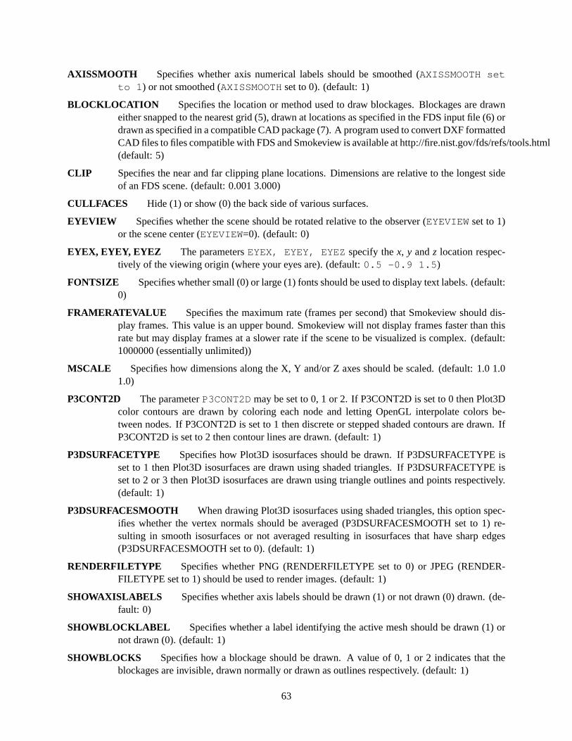
AXISSMOOTH Specifies whether axis numerical labels should be smoothed (AXISSMOOTH setto 1 ) or not smoothed (AXISSMOOTHset to 0). (default: 1)
BLOCKLOCATION Specifies the location or method used to draw blockages. Blockages are drawneither snapped to the nearest grid (5), drawn at locations as specified in the FDS input file (6) ordrawn as specified in a compatible CAD package (7). A program used to convert DXF formattedCAD files to files compatible with FDS and Smokeview is available at http://fire.nist.gov/fds/refs/tools.html(default: 5)
CLIP Specifies the near and far clipping plane locations. Dimensions are relative to the longest sideof an FDS scene. (default: 0.001 3.000)
CULLFACES Hide (1) or show (0) the back side of various surfaces.
EYEVIEW Specifies whether the scene should be rotated relative to the observer (EYEVIEWset to 1)or the scene center (EYEVIEW=0). (default: 0)
EYEX, EYEY, EYEZ The parametersEYEX, EYEY, EYEZ specify thex, y andz location respec-tively of the viewing origin (where your eyes are). (default:0.5 -0.9 1.5 )
FONTSIZE Specifies whether small (0) or large (1) fonts should be used to display text labels. (default:0)
FRAMERATEVALUE Specifies the maximum rate (frames per second) that Smokeview should dis-play frames. This value is an upper bound. Smokeview will not display frames faster than thisrate but may display frames at a slower rate if the scene to be visualized is complex. (default:1000000 (essentially unlimited))
MSCALE Specifies how dimensions along the X, Y and/or Z axes should be scaled. (default: 1.0 1.01.0)
P3CONT2D The parameterP3CONT2Dmay be set to 0, 1 or 2. If P3CONT2D is set to 0 then Plot3Dcolor contours are drawn by coloring each node and letting OpenGL interpolate colors be-tween nodes. If P3CONT2D is set to 1 then discrete or stepped shaded contours are drawn. IfP3CONT2D is set to 2 then contour lines are drawn. (default: 1)
P3DSURFACETYPE Specifies how Plot3D isosurfaces should be drawn. If P3DSURFACETYPE isset to 1 then Plot3D isosurfaces are drawn using shaded triangles. If P3DSURFACETYPE isset to 2 or 3 then Plot3D isosurfaces are drawn using triangle outlines and points respectively.(default: 1)
P3DSURFACESMOOTH When drawing Plot3D isosurfaces using shaded triangles, this option spec-ifies whether the vertex normals should be averaged (P3DSURFACESMOOTH set to 1) re-sulting in smooth isosurfaces or not averaged resulting in isosurfaces that have sharp edges(P3DSURFACESMOOTH set to 0). (default: 1)
RENDERFILETYPE Specifies whether PNG (RENDERFILETYPE set to 0) or JPEG (RENDER-FILETYPE set to 1) should be used to render images. (default: 1)
SHOWAXISLABELS Specifies whether axis labels should be drawn (1) or not drawn (0) drawn. (de-fault: 0)
SHOWBLOCKLABEL Specifies whether a label identifying the active mesh should be drawn (1) ornot drawn (0). (default: 1)
SHOWBLOCKS Specifies how a blockage should be drawn. A value of 0, 1 or 2 indicates that theblockages are invisible, drawn normally or drawn as outlines respectively. (default: 1)
63

SHOWCEILING Specifies whether the ceiling (upper bounding surface) should be drawn (1) or notdrawn (0). (default: 0)
SHOWCOLORBARS Specifies whether the color bars should be drawn (1) or not drawn (0). (default:1)
SHOWFLOOR Specifies whether the floor (lower bounding surface) should be drawn (1) or not drawn(0). (default: 1)
SHOWFRAME Specifies whether the frame surrounding the scene should be drawn (1) or not drawn(0). (default: 1)
SHOWFRAMELABEL Specifies whether the frame number should be drawn (1) or not drawn (0).(default: 1)
SHOWFRAMERATE Specifies whether the frame rate label should be drawn (1) or not drawn (0).(default: 0)
SHOWLABELS Specifies whether labels should be drawn (1) or not drawn (0). Labels are specifiedusing theLABEL keyword described in subsection 4.10. (default: 0)
SHOWMEMLOAD Specifies (when run on a PC) whether a label giving the memory used should bedrawn (1) or not drawn (0). (default: 0)
SHOWNORMALWHENSMOOTH Specifies that smooth blocks should be drawn as normal blocks(1) or drawn as smooth blocks (0). (default: 0)
SHOWOPENVENTS Specifies that open vents should be drawn (1) or not drawn (0). (default: 0)
SHOWDUMMYVENTS Specifies that dummy vents (vents created by FDS) should be drawn (1) ornot drawn (0). (default: 0)
SHOWSMOKEPART Specifies whether smoke or trace particles should be drawn (1) or not drawn(0). (default: 1)
SHOWSPRINKPART Specifies whether sprinkler droplet particles (if present in the particle file) shouldbe drawn (1) or not drawn (0). (default: 1)
SHOWTICKS Specifies whether labels should be drawn (1) or not drawn (0). Ticks are specified usingtheTICK keyword described in subsection 4.10. (default: 0)
SHOWTIMEBAR Specifies whether the timebar should be drawn (1) or not drawn (0). (default: 1)
SHOWTIMELABEL Specifies whether the time label should be drawn (1) or not drawn (0). (default:1)
SHOWHMSTIMELABEL Specifies whether the time label should be drawn (1) or not drawn (0) usingthe format “h:m:s” where “h” is hours, “m” is minutes and “s” is seconds. (default: 0)
SHOWTITLE Specifies whether the title should be drawn (1) or not drawn (0). (default: 1)
SHOWVENTS Specifies whether vents should be drawn (1) or not drawn (0). (default: 1)
SHOWWALLS Specifies whether the four walls (four vertical bounding surfaces) should be drawn (1)or not drawn (0). (default: 1)
STARTUPVIEW Used by Smokeview to record the view to be displayed at startup (as defined in aprevious Smokeview run).
SURFINC Smokeview allows one to display two Plot3D isosurfaces simultaneously. The SURFINCparameter specifies the interval between displayed Plot3D surface values. (default: 0)
64

TIMEOFFSET Specifies that offset time in seconds added to the displayed simulation time. Along withtheSHOWHMSTIMELABEL keyword, theTIMEOFFSET keyword allows one to display“wall clock” rather than simulation time. (default: 0.0)
TITLESAFE Amount in pixels to offset titles when displaying scene in “title safe” mode. (default: 0)
TRANSPARENT Specifies whether 2D and 3D contours should be drawn with solid colors (0) ortransparent colors(1). (default: 1)
UNIT This keyword defines how to calculate colorbar label values for non-default units. Note that inthe following example all text to the right of the ‘//‘ characters is not part of the keyword but isused to explain the format.
default:
UNITtemperature // text appearing in smokeview unit menu1 // number of FDS variables that have temperature unitstemp // FDS variable, appears in colorbar heading3 1 // number of units, default unit numberC // first unit1.0 0.0 // newunitval = 1.0*oldunitval + 0.0F // second unit1.8 32.0K // third unit1.0 273.15
UNITvelocity // text appearing in smokeview unit menu4 // number of FDS variables that have velocity unitsU-VEL // first variableV-VEL // second variableW-VEL // third variableSpeed // fourth variable3 1 // number of units, default unit numberm/s1.0 0.0mph2.236932 0.0f/s3.280833 0.0
VECTORSKIP Specifies what vectors to draw. For example, if this parameter is set to 2 then every2nd vector is drawn when displaying vectors. (default: 1)
VIEWPOINT Specifies the internal Smokeview parameters used to record a scene’s viewpoint and ori-entation. This parameter is set automatically by Smokeview when a .ini file is created. (default:none)
XYZCLIP Specifies clip planes in physical coordinates. There are six clipping planes, a minimum andmaximum X, a minimum and maximum Y, a minimum and maximum Z. Each clipping planemay be used or not. The first parameter is 1 or 0 and specifies whether clipping is turned on oroff. The next three lines specify clipping parameters for the X, Y and Z axes. Each line has theformat
65
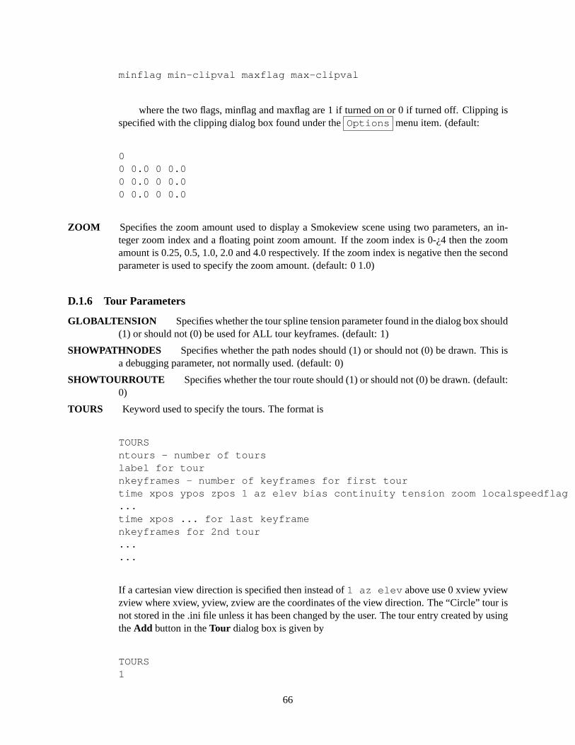
minflag min-clipval maxflag max-clipval
where the two flags, minflag and maxflag are 1 if turned on or 0 if turned off. Clipping isspecified with the clipping dialog box found under theOptions menu item. (default:
00 0.0 0 0.00 0.0 0 0.00 0.0 0 0.0
ZOOM Specifies the zoom amount used to display a Smokeview scene using two parameters, an in-teger zoom index and a floating point zoom amount. If the zoom index is 0-¿4 then the zoomamount is 0.25, 0.5, 1.0, 2.0 and 4.0 respectively. If the zoom index is negative then the secondparameter is used to specify the zoom amount. (default: 0 1.0)
D.1.6 Tour Parameters
GLOBALTENSION Specifies whether the tour spline tension parameter found in the dialog box should(1) or should not (0) be used for ALL tour keyframes. (default: 1)
SHOWPATHNODES Specifies whether the path nodes should (1) or should not (0) be drawn. This isa debugging parameter, not normally used. (default: 0)
SHOWTOURROUTE Specifies whether the tour route should (1) or should not (0) be drawn. (default:0)
TOURS Keyword used to specify the tours. The format is
TOURSntours - number of tourslabel for tournkeyframes - number of keyframes for first tourtime xpos ypos zpos 1 az elev bias continuity tension zoom localspeedflag...time xpos ... for last keyframenkeyframes for 2nd tour......
If a cartesian view direction is specified then instead of1 az elev above use 0 xview yviewzview where xview, yview, zview are the coordinates of the view direction. The “Circle” tour isnot stored in the .ini file unless it has been changed by the user. The tour entry created by usingtheAdd button in theTour dialog box is given by
TOURS1
66
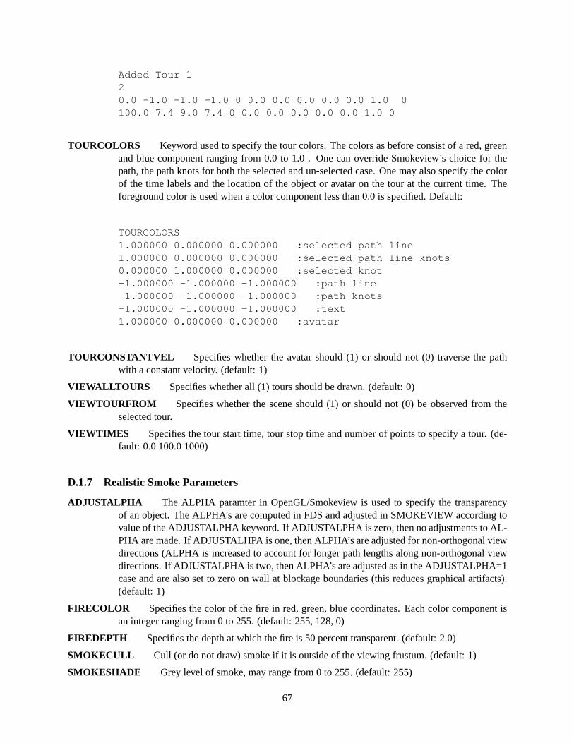
Added Tour 120.0 -1.0 -1.0 -1.0 0 0.0 0.0 0.0 0.0 0.0 1.0 0100.0 7.4 9.0 7.4 0 0.0 0.0 0.0 0.0 0.0 1.0 0
TOURCOLORS Keyword used to specify the tour colors. The colors as before consist of a red, greenand blue component ranging from 0.0 to 1.0 . One can override Smokeview’s choice for thepath, the path knots for both the selected and un-selected case. One may also specify the colorof the time labels and the location of the object or avatar on the tour at the current time. Theforeground color is used when a color component less than 0.0 is specified. Default:
TOURCOLORS1.000000 0.000000 0.000000 :selected path line1.000000 0.000000 0.000000 :selected path line knots0.000000 1.000000 0.000000 :selected knot-1.000000 -1.000000 -1.000000 :path line-1.000000 -1.000000 -1.000000 :path knots-1.000000 -1.000000 -1.000000 :text1.000000 0.000000 0.000000 :avatar
TOURCONSTANTVEL Specifies whether the avatar should (1) or should not (0) traverse the pathwith a constant velocity. (default: 1)
VIEWALLTOURS Specifies whether all (1) tours should be drawn. (default: 0)
VIEWTOURFROM Specifies whether the scene should (1) or should not (0) be observed from theselected tour.
VIEWTIMES Specifies the tour start time, tour stop time and number of points to specify a tour. (de-fault: 0.0 100.0 1000)
D.1.7 Realistic Smoke Parameters
ADJUSTALPHA The ALPHA paramter in OpenGL/Smokeview is used to specify the transparencyof an object. The ALPHA’s are computed in FDS and adjusted in SMOKEVIEW according tovalue of the ADJUSTALPHA keyword. If ADJUSTALPHA is zero, then no adjustments to AL-PHA are made. If ADJUSTALHPA is one, then ALPHA’s are adjusted for non-orthogonal viewdirections (ALPHA is increased to account for longer path lengths along non-orthogonal viewdirections. If ADJUSTALPHA is two, then ALPHA’s are adjusted as in the ADJUSTALPHA=1case and are also set to zero on wall at blockage boundaries (this reduces graphical artifacts).(default: 1)
FIRECOLOR Specifies the color of the fire in red, green, blue coordinates. Each color component isan integer ranging from 0 to 255. (default: 255, 128, 0)
FIREDEPTH Specifies the depth at which the fire is 50 percent transparent. (default: 2.0)
SMOKECULL Cull (or do not draw) smoke if it is outside of the viewing frustum. (default: 1)
SMOKESHADE Grey level of smoke, may range from 0 to 255. (default: 255)
67
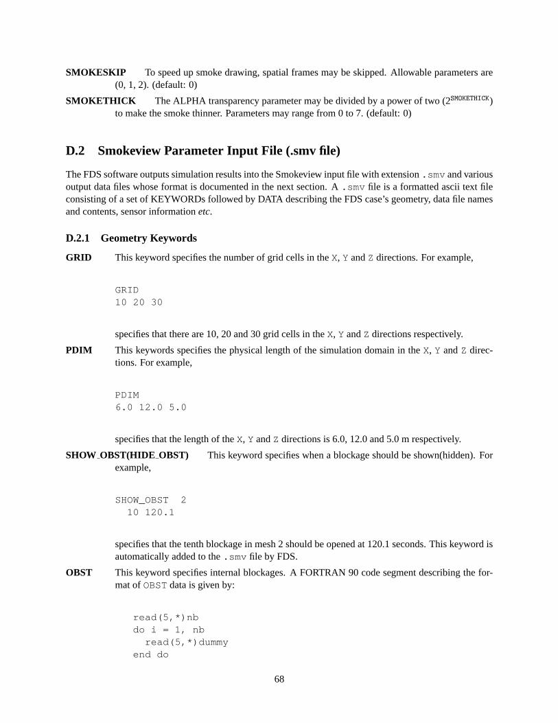
SMOKESKIP To speed up smoke drawing, spatial frames may be skipped. Allowable parameters are(0, 1, 2). (default: 0)
SMOKETHICK The ALPHA transparency parameter may be divided by a power of two (2SMOKETHICK)to make the smoke thinner. Parameters may range from 0 to 7. (default: 0)
D.2 Smokeview Parameter Input File (.smv file)
The FDS software outputs simulation results into the Smokeview input file with extension.smv and variousoutput data files whose format is documented in the next section. A.smv file is a formatted ascii text fileconsisting of a set of KEYWORDs followed by DATA describing the FDS case’s geometry, data file namesand contents, sensor informationetc.
D.2.1 Geometry Keywords
GRID This keyword specifies the number of grid cells in theX, Y andZ directions. For example,
GRID10 20 30
specifies that there are 10, 20 and 30 grid cells in theX, Y andZ directions respectively.
PDIM This keywords specifies the physical length of the simulation domain in theX, Y andZ direc-tions. For example,
PDIM6.0 12.0 5.0
specifies that the length of theX, Y andZ directions is 6.0, 12.0 and 5.0 m respectively.
SHOW OBST(HIDE OBST) This keyword specifies when a blockage should be shown(hidden). Forexample,
SHOW_OBST 210 120.1
specifies that the tenth blockage in mesh 2 should be opened at 120.1 seconds. This keyword isautomatically added to the.smv file by FDS.
OBST This keyword specifies internal blockages. A FORTRAN 90 code segment describing the for-mat ofOBSTdata is given by:
read(5,*)nbdo i = 1, nb
read(5,*)dummyend do
68
do i = 1, nbread(5,*)ib1(i), ib2(i), jb1(i), jb2(i), kb1(i), kb2(i)
end do
whereib1, ib2, jb1, jb2, kb1, kb2 are integer arrays containing boundary nodes.
TRNX,TRNY,TRNZ TheTRNX, TRNY, TRNZkeywords specify grid nodes in theX, Y, Z coor-dinate directions. A FORTRAN 90 code segment describing the format ofTRNXdata is givenby:
read(5,*)nxdo i = 1, nx
read(5,*)idummyend dodo i = 1, nx
read(5,*)xplt(i)end do
TRNYandTRNZdata entries are defined similarly. The firstnx data items are not required bySmokeview.
VENT The keyword specifies vent coordinates. A FORTRAN 90 code segment describing the formatof VENTdata is given by:
read(5,*)nvdo i = 1, nv
read(5,*)dummyend dodo i = 1, nv
read(5,*)iv1(i), iv2(i), jv1(i), jv2(i), kv1(i), kv2(i)end do
whereiv1, iv2, jv1, jv2, kv1, kv2 are integer arrays containing vent coordinates.
OPEN VENT(CLOSE VENT) This keyword specifies when a vent should be opened(closed). Forexample,
OPEN_VENT 23 15.6
specifies that the third vent in mesh 2 should be opened at 15.6 S.
XYZ TheXYZkeyword defines the .xyz orPlot3D grid file name. A FORTRAN 90 code segmentdescribing the format ofXYZdata is given by:
read(5,"(a)")xyzfilename
69
wherexyzfilename is a character variable containing the name of the .xyz file.
D.2.2 File Keywords
BNDF TheBNDFkeyword defines the.bf file name along with character labels used to describe thedata contents of the boundary file.
INPF TheINPF keyword specifies a file containing a copy of the FDS input file.
ISOF TheISOF keyword defines the.iso file name along with character labels used to describe thedata contents of the isosurface file.
PART ThePARTkeyword defines the.part file name along with character labels used to describethe data contents of the particle file.
PL3D The PL3D keyword defines the.q file name along with character labels used to describe thedata contents for each Plot3D variable.
SLCF TheSLCFkeyword defines the.sf file name along with character labels used to describe thedata contents of the slice file.
D.2.3 Sensor Keywords
HEAT TheHEATkeyword defines heat detector location data. A FORTRAN 90 code segment describ-ing the format ofHEATdata is given by:
read(5,*)nheatdo i = 1, nheat
read(5,*)xheat(i),yheat(i),zheat(i)end do
wherenheat is the number of heat detectors andxheat, yheat, zheat are thex, y,z coordinates of the heat detectors.
HEAT ACT The HEATACT keyword defines heat detector activation data. A FORTRAN 90 codesegment describing the format ofHEATACTdata is given by:
read(5,*)iheat, heat_time
whereheat time is the activation time of theiheat ’th heat detector.
SPRK TheSPRKkeyword defines sprinkler location data. A FORTRAN 90 code segment describingthe format ofSPRKdata is given by:
read(5,*)nsprinkdo i = 1, nsprink
read(5,*)xsprink(i),ysprink(i),zsprink(i)end do
70
wherensprink is the number of sprinklers andxsprink, ysprink, zsprink are thex, y, z coordinates of the sprinklers.
SPRK ACT TheSPRKACTkeyword defines sprinkler activation data. A FORTRAN 90 code segmentdescribing the format ofSPRKACTdata is given by:
read(5,*)isprink, sprink_time
wheresprink time is the activation time of theisprink ’th sprinkler.
THCP The THCPkeyword defines thermocouple location data. A FORTRAN 90 code segment de-scribing the format ofTHCPdata is given by:
read(5,*)nthermdo i = 1, ntherm
read(5,*)xtherm(i),ytherm(i),ztherm(i)end do
wherentherm is the number of thermocouples andxtherm, ytherm and ztherm arethex, y and z coordinates of the thermocouples.
D.2.4 Miscellaneous Keywords
ENDIAN TheENDIANkeyword defines whether a big or little endian4 system is used to represent thedata. The PC (both Windows and LINUX) uses the little endian system for representing num-bers while most UNIX workstations use the big endian system. The PC version of Smokeviewuses this keyword to determine whether data should be converted between these two systemsbefore it is visualized. The validENDIANparameters areBIG or LITTLE .
SYST TheSYSTkeyword defines which system the FDS case was run on. The PC version of Smoke-view uses this information (if theENDIAN keyword is absent) to swap data bytes if the FDScase was run on a computer with a different “endian” format than the PC.
TITLE1/TITLE2 TheTITLE1 andTITLE2 keywords allow one to specify extra information docu-menting a Smokeview case. These keywords and associated labels are added by hand to thesmokeview (.smv) file using the format:
TITLE1first line of descriptive textTITLE2second line of descriptive text
4Big-endian and little-endian are terms that describe the order in which a sequence of bytes are stored in computer memory.Big-endian is an order in which thebig end(most significant value in the sequence) is stored first (at the lowest storage address).Little-endian is an order in which thelittle end (least significant value in the sequence) is stored first. The terms big-endian andlittle-endian are derived from the Lilliputians of Gulliver’s Travels, whose major political issue was whether soft-boiled eggs shouldbe opened on the big end or the little end.
71

D.3 Data File Formats (.s3d, .iso, .part, .sf, .bf and .q files)
Smokeview visualizes Fire Dynamics Simulator data using isosurface, particle, boundary, slice and Plot3Ddata files described in this section along with a Smokeview parameter input file described in the previoussection. This section documents the data format of each data file by showing FORTRAN program codesegments used to write the data out. All files are unformatted and are opened usingOPENstatements of theform:
OPEN(UNIT=IUNIT,FILE=FILENAME,FORM="UNFORMATTED")
whereIUNIT is the FORTRAN unit number used for output andFILENAMEis a character variable contain-ing the file name. In the following code segments the standard FORTRAN naming convention of associatingvariables beginning with I through N to integer variables and all other alphabetic characters to REAL vari-ables is used. It is assumed that all variables take up four bytes. Variables having DUMMY in the nameindicates that they are not used by Smokeview.
D.3.1 3D Smoke File Format
D.3.2 Isosurface File Format
Isosurface files are used to store one or more surfaces where each surface represents a region where thesolution take one a particular value. The FDS software outputs isosurface frames at fixed time intervals.Note that char’s are one byte, short’s are two bytes and “int’s” and float’s are four bytes. A “pseudo-code”representation of the isosurface file is given by:
version (int)len1,len2,len3 (3*int)label1,label2,label3 ((len1+len2+len3+4)*char)nlevels (int)level_1, level_2, ..., level_nlevels (nlevels*float)for each time:
time (float)for each level
nvertices (int)ntriangles (int)vertices_1, ..., vertex_nvertices (3*short*nvertices)triangles_1, ..., triangle_ntriangles (3*(byte/short/float)*ntriangles)
end levelend time
The length of eachtriangles i node is one byte if the number of triangles,ntriangles , isbetween zero and 255 (inclusive), two bytes ifntriangles is between 256 and 65536 (inclusive) andfour bytes ifntriangles is greater than or equal to 65536. Note that the isosurface files are written usingthe C programming language. These files should be read the same way unless the programming language ofchoice supports binary I/O.
D.3.3 Particle File Format
Particle files are used to store smoke/tracer particles and/or sprinkler droplet information. The particle fileconsists of a header and a series of particle frames. Each frame contains particle/droplet positions and data
72
values for each particle in that frame. The FDS software outputs particle frames at fixed time intervals butthere is no requirement by Smokeview for this to happen. Smokeview reads in the data one frame at a timenoting the time read in for each frame. The header can be described using the code segment:
WRITE(IUNIT) DUMMY,DUMMY,DUMMY,IPART,NPPSWRITE(IUNIT) IBAR,JBAR,KBARWRITE(IUNIT) (DUMMY,I=0,IBAR),(DUMMY,J=0,JBAR),(DUMMY,K=0,KBAR)WRITE(IUNIT) NBDO N=1,NB
WRITE(IUNIT) IB1(N),IB2(N),JB1(N),JB2(N),KB1(N),KB2(N),1END DOWRITE(IUNIT) NVDO N=1,NV
WRITE(IUNIT) IV1(N),IV2(N),JV1(N),JV2(N),KV1(N),KV2(N),2END DOWRITE(IUNIT) NSPRDO N=1,NSPR
WRITE(IUNIT) XSP0(N),YSP0(N),ZSP0(N)END DO
whereDUMMYis written by FDS but not needed by Smokeview,IPART is the index of the scalar quantityassociated with the particles,NPPSis the maximum number of particles per frame,IB1, IB2, etcare theindices of blocked grid cells,IV1, IV2, etc indicate vent cell nodes, andXSP0, YSP0, ZSP0 are thecoordinates of the sprinklers. Grid coordinates are obtained by Smokeview from the Smokeview parameterinput file. A particle frame is written using:
WRITE(IUNIT) TIME,NP,IDUMMY,(ISPR(N),N=1,NSPR)WRITE(IUNIT) (XP(I),I=1,NP),
. (YP(I),I=1,NP),
. (ZP(I),I=1,NP),
. (BP(I),I=1,NP)IF (NASPR.GT.0) THEN
WRITE(IUNIT) NSPWRITE(IUNIT) (XSP(I),I=1,NSP),(YSP(I),I=1,NSP),(ZSP(I),I=1,NSP)
ENDIF
whereNPis the number of particles in this frame,ISPR denotes whether the sprinkler has activated,NSPRis the number of sprinklers,XP, YP, ZP are the particle coordinates,BP is the particle value,NASPRisthe number of active sprinklers,NSP is the number of sprinkler droplets, andXSP, YSP, ZSP are thedroplet coordinates.
D.3.4 Slice File Format
Slice files are unformatted. The slice file header is written out using:
WRITE(IUNIT) CDUMMYWRITE(IUNIT) CDUMMYWRITE(IUNIT) CDUMMYWRITE(IUNIT) I1,I2,J1,J2,K1,K2
73
whereCDUMMYis a character strings of length 30. Smokeview obtains this information from the Smoke-view parameter input file and not from the slice file. The sextuple (I1,I2,J1,J2,K1,K2 ) denotes thebounding grid cell nodes of the slice to be displayed. The sextuple indices correspond to grid cell nodes, orcorners, thus the entire grid would be represented by the sextuple (0,IBAR,0,JBAR,0,KBAR ). The gridnode positions are obtained from the Smokeview parameter input file.
The FDS software outputs slice frames at fixed time intervals but there is no requirement by Smokeviewfor this to happen. Each slice frame is written using:
WRITE(IUNIT) TIMEWRITE(IUNIT) (((QQ(I,J,K),I=11,I2),J=J1,J2),K=K1,K2)
whereTIME is the time in seconds when the data is ouput andQQare the data values.
D.3.5 Boundary Files
The boundary files are unformatted. The header is written out using:
WRITE(IUNIT) QUANTITYWRITE(IUNIT) SHORT_NAMEWRITE(IUNIT) UNITSWRITE(IUNIT) NPATCHDO 10 I=1,NPATCH
WRITE(IUNIT) IP1(I),IP2(I),JP1(I),JP2(I),KP1(I),KP2(I)10 CONTINUE
whereQUANTITY, SHORTNAMEandUNITS are character strings of length 30,NPATCHis the numberof planes (or “patches”) that make up the solid boundaries plus the external walls. The sextuple arrays(IP1,IP2,JP1,JP2,KP1,KP2 ) defines the cell nodes of each patch. The user does not prescribe these.
The FDS software outputs boundary frames at fixed time intervals but there is no requirement by Smoke-view for this to happen. The boundary file frame is written using:
WRITE(IUNIT) TIMEDO 10 I=1,NPATCH
WRITE(IUNIT) (((QQ(I,J,K),I=IP1(I),IP2(I)),J=JP1(I),JP2(I)),K=KP1(I),KP2(I))10 CONTINUE
D.3.6 Plot3D Data
Field data is dumped periodically by FDS in a format used by the graphics packagePlot3D[17]. ThePlot3D data sets are single precision (32 bit reals), whole and unformatted. Note that there is blanking, thatis, blocked out data points are not plotted. The grid data is written out to a file calledcasename.xyzusing:
WRITE(IUNIT) IBAR+1,JBAR+1,KBAR+1WRITE(IUNIT) (((X(I),I=0,IBAR),J=0,JBAR),K=0,KBAR),
. (((Y(J),I=0,IBAR),J=0,JBAR),K=0,KBAR),
. (((Z(K),I=0,IBAR),J=0,JBAR),K=0,KBAR),
. (((IBLK(I,J,K),I=0,IBAR),J=0,JBAR),K=0,KBAR)
74
whereIBAR+1, JBAR+1, KBAR+1 are the number of grid cells along theI, J, K coordinate direc-tions,X, Y andZ are the physical coordinates of the cell corners, andIBLK is an indicator of whether ornot the cell is blocked. If the point (X,Y,Z ) is completely embedded within a solid region, thenIBLK is 0.Otherwise,IBLK is 1. The flow variables are written to a file using:
WRITE(IUNIT) IBAR+1,JBAR+1,KBAR+1WRITE(IUNIT) ZERO,ZERO,ZERO,ZEROWRITE(IUNIT) ((((QQ(I,J,K,N),I=0,IBAR),J=0,JBAR),K=0,KBAR),N=1,5)
The five channelsN=1,5 are by default the temperature (C), theu, v andw components of the velocity(m/s), and the heat release rate per unit volume (kW/m3).
75

76
Appendix E
Frequently Asked Questions
This appendix contains a list of frequently asked questions concerning Smokeview. An updated list may befound at http://fire.nist.gov/smokeview .
E.1 How can I keep up with new releases and other information about FDSand Smokeview?
An e-mail list has been set up to alert users to changes, upgrades,etc. To subscribe to the list, send an emailto [email protected] and put the line
subscribe fdsusers Jane Doe
in the text where Jane Doe is your name. Subject line is unimportant. To get off the list, send an emailto the same address and write
unsubscribe fdsusers
Also, you can check the web page http://fire.nist.gov/download to see the date of the most recent update.
E.2 Can I run Smokeview on other machines?
Smokeview is more complicated to compile on other platforms because it uses several freeware librariesthat need to be compiled and installed on that particular machine. We have compiled Smokeview on thePC, SGI (IRIX), and Red Hat Linux, but with the exception of the PC executable, there’s no guarantee thatsomething we compile on one of our machines is going to work on yours. Worse comes to worse, use a PCto visualize the output of a calculation run on your other machine.
E.3 Smokeview doesn’t look right on my computer. What’s wrong?
Some video cards do not use enough bits to represent the “depth buffer”. The depth buffer is used todetermine when objects are hidden and therefore should not be drawn. A problem then can occur when thevideo card reduces the number of depth buffer bits from 32 to 16 in order to speed up its performance (lessdata to transport). This results in straight lines or polygonal edges appearing to be scalloped. Often reducingthe acceleration setting for the video card can eliminate this problem. To do this:
• click your mouse on the desktop to bring up the ”Display Properties” dialog box.
77
• click on the ”Advanced...” button
• Find the dialog panel that lets you select the ”Hardware acceleration”. Reduce the acceleration (re-booting if necessary) until the scalloping disappears.
If you have upgraded your PC recently, make sure you have loaded the latest drivers for your video card.
E.4 How do I make a movie of a Smokeview animation?
You make a movie of a Smokeview animation by converting the visualized scene into a series of PNG orJPEG files, one file for each time. More specifically:
• Set up Smokeview orienting the scene and loading the desired data files.
• Select theOptions/Render menu and pick the desired frame rate. The more frames you includein the animation, the smoother it will look. Of course more frames results in larger file sizes.
• Use a program such as the Antechinus Media Editor or Platypus Animator available at http://www.c-point.com
E.5 Smokeview is running much slower than I expected. What can I do?
A likely explanation is that your video drivers are not hardware accelerated for OpenGL. You need to down-load the latest drivers for your video card. You may also try playing around with the hardware acclerationsettings (see E.3).
E.6 I loaded a particle file but Smokeview is not displaying particles. Whatis wrong?
This is a bug in your video card. To see particles, reduce your hardware acceleration setting (see E.3).
78