user's guide to reproduce calculations in: technical ... · user’s guide to reproduce...

Cambridge, MA Lexington, MA Hadley, MA Bethesda, MD Chicago, IL

User’s Guide to Reproduce Calculations in: Technical Report on Ozone Exposure, Risk, and Impact Assessments for Vegetation July 20, 2007 Prepared for Vicki Sandiford US EPA / OAQPS Prepared by Melanie Bacou Jonathan A. Lehrer Brian Blankespoor Jason Sacks Don McCubbin Work funded through Contract 68-D-03-002 Work Assignment 4-61

User’s Guide to Reproduce Calculations in: Technical Report on Ozone Exposure, Risk,

and Impact Assessments for Vegetation

Abt Associates Inc. i

Table of Contents List of Tables ................................................................................................................................................ii

List of Figures ...............................................................................................................................................ii

Introduction................................................................................................................................................... 1 *** If you don’t read any other part of this file, read this: *** ................................................................ 1 Configuring SAS and SQL Server ............................................................................................................ 2

1 Potential Ozone Exposure Surface........................................................................................................ 3 1.1 Unpack Raw Data........................................................................................................................ 3

1.1.1 AQS Data ................................................................................................................................ 4 1.1.2 CASTNet................................................................................................................................. 6 1.1.3 CMAQ..................................................................................................................................... 6

1.2 Prepare VNATool for First Use................................................................................................... 6 1.3 Generate As-Is Potential Ozone Surface...................................................................................... 6 1.4 Rollback POES to Simulate Meeting Several Air Quality Standards ......................................... 7 1.5 Calculate Summary Metrics of Rollback Scenarios and Combine East and West Data ............. 8

2 Crop Yield and Tree Seedling Biomass Impacts .................................................................................. 8 2.1 Prepare SQL Server for First Use................................................................................................ 9 2.2 Gather All Input Data ................................................................................................................ 10

2.2.1 Input Tables Pre-Loaded in the OZONE SQL Database ...................................................... 10 2.2.2 Load Monthly As-Is and Rollback POES into the SQL Database......................................... 14

2.3 Generate Estimated Percent Changes in Crop Yield and Tree Seedling Biomass due to Ozone .. ................................................................................................................................................... 14 2.4 Prepare Input Data for AGSIM ................................................................................................. 15 2.5 Prepare Input Data for TREGRO .............................................................................................. 16 2.6 Prepare Input Data for ArcGIS Maps ........................................................................................ 16 2.7 Compute Summary Statistics..................................................................................................... 17

List of References ....................................................................................................................................... 20

Glossary of Terms....................................................................................................................................... 21

Abt Associates Inc. ii

List of Tables Table 1: Crosswalk between Sections of the User’s Guide and Chapters and Sections of the Technical

Report.................................................................................................................................................... 2 Table 2: Input Tables to Estimate Percent Changes in Crop Yield and Tree Seedling Biomass due to

Ozone .................................................................................................................................................. 12 Table 3: Output Tables with Estimates of Percent Changes in Crop Yield and Tree Seedling Biomass Due

to Ozone.............................................................................................................................................. 15 Table 4: Output Variables showing Percent Changes in Crop Yield and Tree Seedling Biomass Due to

Ozone .................................................................................................................................................. 15

List of Figures Figure 1: Directory Structure and Code Files to Replicate Potential Ozone Exposure Surfaces.................. 5 Figure 2: Step 1. Download, Install, and Manually Start SQL Server.......................................................... 9 Figure 3: Step 2. Download, Install, and Start SQL Server Management Studio Express ......................... 10 Figure 4: Step 3. Attach OZONE Database to SQL Server ........................................................................ 11 Figure 5: Input Tables to Replicate Crop Yield and Tree Seedling Biomass Impacts................................ 11 Figure 6: All Code Files to Replicate Crop Yield and Tree Seedling Biomass Impacts ............................ 13 Figure 7: Create a New ODBC Data Source Referencing the SQL “OZONE” Database .......................... 19 Figure 8: Create a New SAS Library Referencing the “OZONE” ODBC Data Source ............................. 19

Abt Associates Inc. 1/25

Introduction This document is intended as a step-by-step guide for anyone who wishes to reproduce the ozone secondary risk assessment performed by Abt Associates under EPA Contract 68-D-03-002. This document should be used in tandem with the January 24, 2007 report entitled Technical Report on Ozone Exposure Risk, and Impact Assessments for Vegetation, and with the accompanying User’s Guide DVD. Generally speaking, the Technical Report on Ozone Exposure Risk, and Impact Assessments for Vegetation (herein refer as the “Technical Report”) describes the study’s motivations, data sources, and methods. The present User’s Guide describes the datasets, tools and code files that were used to carry out the assessment. It also describes how to use these files to replicate the results produced in the Technical Report. The User’s Guide DVD provides the actual code files and input data files used in the analysis. Note that detailed instructions are included in comments at the top of each SAS and SQL code file, and before every important code instruction. We strongly advise the reader to take a look at these comments in addition to the present guide before trying to run the simulations, as some manual adjustments may be needed to ensure the code files run successfully.

*** If you don’t read any other part of this file, read this: ***

1) The entire analysis was carried out using both SAS and Microsoft SQL Server 2005. You will need a user’s license for SAS, and access to a SQL Server in order to replicate the entire analysis. A free version of SQL Server 2005 Express is available for download at http://msdn.microsoft.com/vstudio/express/sql/download/ .

2) In order to replicate the potential ozone exposure surface (POES) and rollback scenarios, you will need to edit the first line of each piece of SAS code before running it. The first line defines a variable mypath, which is the path to the main folder of this package. It may be C:\myprojects\Secondary Ozone Analysis Package\ or any location on your computer where you decide to copy the contents of User’s Guide DVD. The mypath variable is the first line of every SAS code file in the package and you should always set it to the same path.

3) It is best to avoid renaming directories in this package, as much of the code refers to other locations in the file structure. However, if you need to do so, you can usually rectify the situation by editing the first few lines of each SAS code file, where SAS input and output libraries are defined.

4) Top-level folders on the User’s Guide DVD are numbered to follow the logic of the analysis. Hence code files in “1 Generate Potential Ozone Exposure Surface (ch3)” must be run first, before code files in folder “2 Rollback POES to Meet Standards (ch4)” are run. Folder names also indicate the corresponding chapter of the Technical Report.

5) Within each top-level folder, all code files have file names specifying the order in which they must be run. If there are no numbers, then the code can be run in any order.

http://msdn.microsoft.com/vstudio/express/sql/download/


6) This code is time and data intensive! Plan for multiple days and 30-40 GB of free hard drive space.

Table 1 below indicates which chapters of the Technical Report to refer to for each section of the User’s Guide.

Table 1: Crosswalk between Sections of the User’s Guide and Chapters and Sections of the Technical Report

User’s Guide Technical Report 1.1 Unpack Raw Data Chapter 2 1.2 Prepare VNATool for First Use Chapter 3.4 1.3 Generate As-Is Potential Ozone

Surface Chapter 3.4

1.4 Rollback POES to Simulate Meeting Several Air Quality Standards

Chapter 4

1.5 Calculate Summary Metrics of Rollback Scenarios and Combine East and West Data

Chapter 4.3

2.3 Generate Concentration Responses for Crops and Tree Seedlings

Chapter 5

2.4. Prepare Data for AGSIM Chapter 6 2.5. Prepare Data for TREGRO Chapter 7

Configuring SAS and SQL Server

The first part of the analysis (i.e. Chapters 2 through 4 of the Technical Report) was coded entirely in SAS. All SAS code files (*.sas) and input datasets (*.sas7bdat) are provided in the accompanying User’s Guide DVD. You will need a copy of the SAS 9.0 (or above) software in order to generate the POES and the rollback scenarios.1 The second part of the analysis (i.e. Chapter 5 through 7 of the Technical Report) uses a combination of SAS and SQL Server. 2 A free version of SQL Server is available from the Microsoft website at http://msdn.microsoft.com/vstudio/express/sql/download/. You will need to attach the SQL database provided in the User’s Guide DVD and run all SQL code files sequentially in order to replicate the results in Chapter 5. Further instructions are provided in Section 2 below. The impacts of crop yield and tree seedling biomass changes (Chapters 6 and 7) were produced using two stand-alone models, AGSIM (large-scale econometric simulation model of regional crop and national livestock production in the U.S., see Taylor 1993) and TREGRO (physical model simulating responses of plants to interacting stresses, Weinstein 2002). The AGSIM model is included on the User’s Guide DVD at [\4 Compute Crop Yield and Tree Seedling Biomass Changes (ch5)\Code\Step 3. Prepare Input Data for AGSIM\AGSIMEPA.v.01.13.2005.xls]. TREGRO is not publicly available, but you may find further information on-line at http://eco.wiz.uni-kassel.de/model_db/mdb/tregro.html. Please refer to Appendices I and J of the Technical Report for detailed model documentation.

1The included code has not been tested with older SAS versions, although the authors expect it to work on those

versions as well. 2 SAS is generally slower than relational databases to perform lookups over very large datasets, hence the decision

to use a combination of two statistical and modeling tools.


http://eco.wiz.uni-kassel.de/model_db/mdb/tregro.html


The remainder of the User’s Guide is organized as follows. Section 1 outlines the steps used to generate Eastern and Western POES and “rolled-back POES”. Section 2 describes the steps used to replicate crop yield and tree seedling biomass changes resulting from the POES obtained in Sections 1, as well as the steps needed to prepare input datasets to feed into the AGSIM and TREGRO models. Finally section 2 provides instructions and input layers to reproduce the air quality maps and crop yield and tree seedling biomass impact maps published in the Technical Report.

1 Potential Ozone Exposure Surface The assessment begins with generating a Potential Ozone Exposure Surface, which provides ozone values at each point in a regularly-spaced grid covering the continental U.S. Because actual monitor coverage in rural areas in the U.S. is sparse, many of the ozone values in the POES are imputed using spatial interpolation techniques. Several techniques for spatial interpolation were evaluated before an approach was chosen for generation the POES. The techniques used and described in section 3.4 of the Technical Report are built in the accompanying code files. Straight VNA interpolation was used for the Eastern U.S., while a VNA-eVNA blend was used in the West. This section describes how to unpack the raw data and run the code used to evaluate the various spatial interpolation techniques. It also explains how to run the code which generates the POES.

1.1 Unpack Raw Data

This section parallels Chapter 2 of the Technical Report. Start by copying the contents of the User’s Guide DVD onto a hard drive with plenty of free space (30 to 40GB). Throughout the rest of the document, we will call the root of the User’s Guide DVD mypath. For example, if you copy the data into C:\AbtOzone\2007 Analysis\, then mypath\Original Raw Data\ refers to C:\AbtOzone\2007 Analysis\Original Raw Data\. On occasion you will need to edit code files to point SAS libraries to the actual path of the input/output data. We will rely heavily on the mypath-notation in these sections. Note: to ensure proper functioning of all SAS code, do not rename subfolders. Often the code will refer to specific subfolders and will fail if they have been renamed. The input data used to generate the POES originates from three sources:

1) Air Quality System (AQS) monitor data

2) Clean Air Status and Trends Network (CASTNet) monitor data

3) Community Multiscale Air Quality (CMAQ) model data

To obtain this data, we used the AQS and CASTNet websites (see Technical Report for details). CMAQ data was provided by EPA in Network Common Data Form (NetCDF) format along with a program to convert the binary file to text. The User’s Guide DVD contains a folder entitled “0. Raw Data (ch2)”. The folder contains three subfolders – one for AQS, one for CASTNet, and one for CMAQ data (Figure 1).


1.1.1 AQS Data In the AQS subfolder, you will find two ZIP files and two SAS code files. Each SAS code file is used to process the data in one of the ZIP files. Unzip the ZIP files into subfolders in the AQS directory. Do not rename the ZIP files and make sure that the subfolders take the exact same name as each ZIP file. For example:

\mypath\ AQS Monitor Data\RD_501_44201_2001.zip gets unzipped into:

\mypath\ AQS Monitor Data\RD_501_44201_2001\ Open each SAS file and replace the mypath placeholder in the first line with the path of the AQS subfolder. For example:

C:\AbtOzone\Original Raw Data\AQS Monitor Data\ Run each SAS file sequentially. This should produce the following output: a SAS dataset entitled AQS_44201 – this contains the hourly ozone observations from AQS monitors.

Figure 1: Directory Structure and Code Files to Replicate Potential Ozone Exposure Surfaces



1.1.2 CASTNet Unzip all ZIP files to the current directory.

1.1.3 CMAQ CMAQ is the trickiest of the three to unpack. In the CMAQ subfolder, you will find two .conc files (binary data files), two .bat files (MS-DOS batch files), and one .exe. Each batch file is designed to convert one of the binary data files into text format. They make use of the .exe program to do this, so all 5 files must be kept in the same directory in order for the conversion to work. Once the data files have been converted to text format, the text files can be moved around at will. Note that the data files are quite large (600 MB and 1.3 GB), and become even larger when converted to text format (7 GB and 16 GB). Make sure you have sufficient disk space before proceeding.3

1.2 Prepare VNATool for First Use

The analyses made use of a stand-alone program implementing several spatial analysis algorithms. This program is called VNATool.exe, and although it does not need to be installed separately (you will find it in the top-level folder /VNATool/), you may need to make adjustments to your system configuration to be able to use it. Open the program VNATool.exe and click the Browse… button in the top right corner. Look at the dropdown list for Files of Type: at the bottom of the dialog. If Text Files is an option, then there is no need to make any system adjustments. Otherwise, do the following:

1) On your PC go to Control Panel -> Administrative Tools -> Data Sources (ODBC)

2) On the User DSN tab, click Add…

3) Select Microsoft Text Driver and click OK

4) Name the Data Source Text Files and click OK

5) Back in the Data Sources main window, click OK to save your changes and exit.

Back in VNATool, if this process was successful, you should now see the Text Files option under the Files of Type dropdown list.

1.3 Generate As-Is Potential Ozone Surface

This section describes how to reproduce the as-is POES of the U.S. in 2001. The POES is used as a main input data for all subsequent steps of the analysis. All code files in this section can be found in the folder 1. Generate Potential Ozone Exposure Surface (ch3). A description of the method used may be found in Chapter 4 of the Technical Report. Note that a slightly different methodology is used in the Eastern U.S. than in the Western U.S. In the Western U.S., CMAQ modeling data is incorporated into the interpolation of monitor data to unmonitored areas. The relevant methodological differences are already built into the code, so no special action is required to implement them, other than running the code in the order specified. See chapter 4 for more details on the two methodologies. There are two subfolders in 1. Generate Potential Ozone Exposure Surface (ch3), one for the Eastern U.S. and one for the Western

3 If needed, the code has been set up so that the initial processing of the western U.S. (which uses the 36km data file)

can be done separately from the initial processing of the eastern U.S. (which uses the 12km data file). Thus, if disk space is lacking, one can unpack only one CMAQ data file at a time, extract the necessary information, and then delete it.


U.S. In each subfolder, there is a Code subfolder containing the SAS code required to generate the POES; and an empty Data folder, which will store the output datasets once the code is run. All SAS code files are numbered in the order in which they need to be run. Note that two code files aren’t actually code – they are text files containing instructions. This is because for the initial part of the analysis, we will make use of the stand-alone VNATool executable to perform spatial analyses. In the code folder:

1) Open the first piece of code, edit the mypath variable, and hit Run.

2) Open VNATool.exe (in its own directory in the User’s Guide DVD package), load the files specified in the instruction file, alter the parameters as instructed, and hit the button as indicated.

3) Open the next piece of code, edit the mypath variable, and hit Run.

4) Open VNATool.exe (in its own directory in the User’s Guide DVD package), load the files specified in the instruction file, alter the parameters as instructed, and hit the button as indicated.



Follow these instructions for both the Eastern U.S. and the Western U.S. folders. At the end of these steps, you will have produced an Eastern POES and a Western POES, as well as several files giving summary metrics of this data. Now it is time to run the rollback procedure, which creates estimated POES representing air quality that meets either the current or alternative standards.

1.4 Rollback POES to Simulate Meeting Several Air Quality Standards

All code in this section can be found in the folder “2 Rollback POES to Meet Standards (ch4)”. A description of the method used can be found in Chapter 4 of the Technical Report. Briefly, the rollback procedure creates estimated POES representing air quality which simulate meeting the current and alternative standards. It shows what hourly air quality might look like if we were able to meet a certain yearly goal for air quality levels. There are two subfolders in the folder “2 Rollback POES to Meet Standards (ch4)”, one for the Eastern U.S. and one for the Western U.S. In each subfolder, there is a Code subfolder containing the code required to generate the POES, and an empty Data subfolder which will store the SAS output datasets once the code is run. Note that the SAS code files in this section are not numbered. This indicates that they can be run in any order you wish. You can also choose to only run code for the rollback scenario that you are interested in. Bear in mind though, that if you do not run all the code you will receive error messages when running code in the next step “3 Calculate Metrics (ch2)”, and you will specifically need to revise the code in [4 Combine East and West.sas] to make it run properly with a partial set of input data, as explained in section 1.5 below. The code is named according to the rollback scenario it generates. For example, [Rollback 8hr 70.sas] performs a rollback of the POES that simulates meeting a 4th-highest 8hr max standard of 70ppb.


Similarly [Rollback W126 21.sas] performs a rollback of the POES to simulate meeting a W126 standard of 21ppm-h. A description of the corresponding method used can be found in Chapter 4 of the Technical Report. To generate any or all of these rollbacks, open the relevant code file(s) in SAS, edit the mypath variable, and hit Run. At the end you will have generated rollback surfaces for all the rollback scenarios for which you have run code. Resulting datasets may be found in the Data subfolder of the appropriate rollback folder.

1.5 Calculate Summary Metrics of Rollback Scenarios and Combine East and West Data

All code for this section may be found in the folder “3 Calculate Metrics (ch2)”. Briefly, the purpose of this code is to take the rollback (and as-is) ozone exposure surfaces, giving hourly ozone data, and to summarize them in terms of monthly or yearly air quality metrics. The code can generate either 10% adjusted or [sic] non-adjusted ozone values as needed. Use the first 2 code files to generate adjusted values, or the next 2 code files to generate unadjusted values (i.e. [2 prepare monthly metrics unreduced by 10pct) East.sas] and [2 prepare monthly metrics (unreduced by 10pct) West.sas]). There are four subfolders in the folder “3 Calculate Metrics (ch2)”: one Code, one for Eastern output data, one for Western output data, and one for the combined data covering the entire continental U.S. SAS code files in the Code subfolder are numbered, but note there are two files for each number up to 3. This is because there is an Eastern and Western version of each file. It does not matter whether you run the Eastern or the Western code file first. Just be sure to edit the mypath variable before hitting Run. If you ran all of the rollback scenarios, you can ignore this paragraph. However, if you did not run all the rollback scenarios, you will need to edit the code file [4 Combine East and West.sas] to avoid errors. This file draws together the files that summarize various rollback procedures into a smaller set of dense files covering the entire U.S. Therefore, for example, if the files for the rollback to simulate meeting a W126 standard of 13ppm-h do not exist (i.e. you did not run this scenario), simply remove all references to that scenario in the code.

2 Crop Yield and Tree Seedling Biomass Impacts This section of the analysis uses a combination of SAS code and SQL code (optimized for Microsoft SQL Server).4 You will need to download and install SQL Server, as well as SQL client program to execute statements against SQL Server, and to load and run SQL code files. Microsoft provides a free version of SQL Server and a free client, SQL Server Management Studio Express, on that same page at http://msdn.microsoft.com/vstudio/express/sql/download/. The data sources and methods used are described in Chapter 5 of the Technical Report. Briefly, we used the monthly ozone data produced in Section 1.5 above as the as-is and rollback POES to 1) generate seasonal ozone indices for each crop and tree species based on growing ranges and typical growing

4 The SQL code uses a number of SQL aggregate functions specific to Microsoft SQL Server, and thus we

recommend you download the free version of SQL Server to replicate the analysis. The input datasets are too large for MS Access, and some of the code will not run in other relational databases such as Oracle and mySQL.


seasons, and 2) compute crop yield impacts, and 3) calculate tree seedling biomass impacts based on species specific concentration-response functions. The resulting data will then serve as input for the AGSIM and TREGRO models respectively. AGSIM is then used to produce a nation-wide assessment of the estimated economic benefits associated with changes in crop yields predicted to occur under alternate air quality scenarios.

2.1 Prepare SQL Server for First Use

Before running the SQL code files, you will first need to import the POES generated in Section 1.5 above into SQL Server. Here are the steps to follow:

1) Install SQL Server Express 2005 (choose the default installation options)

2) Install SQL Server Management Studio Express (SMSE) (choose the default installation options)

3) Start SQL Server ( go to Start -> Microsoft SQL Server 2005 -> SQL Server Configuration Manager, right-click SQL server (SQLEXPRESS) on the right pane, and choose Start, as shown below.

Figure 2: Step 1. Download, Install, and Manually Start SQL Server

You then need to attach (i.e. load) the SQL database provided on the User’s Guide DVD into your SQL Server. Provided you use the free Microsoft SQL client, the step-by-step instructions are as follows:


4) Start SQL Server Management Studio Express from your Start Menu, and connect to your server named .\SQLExpress as shown below. Use either Windows Authentication, or if choose SQL Server Authentication then enter the user name and password you specified when you installed SQL Server.

Figure 3: Step 2. Download, Install, and Start SQL Server Management Studio Express

5) On the left pane, expand the server’s node, right-click on Databases and choose Attach… (Figure 4). Browse to the location where you copied the contents of the User’s Guide DVD, locate the database file at \mypath\4 Compute Crop Yield and Tree Seedling Biomass Changes (ch5)\in\OZONE.mdf, and click OK. You may now start running SQL code files. Note that all datasets produced will be created as new tables inside the OZONE database you just loaded5.

2.2 Gather All Input Data

2.2.1 Input Tables Pre-Loaded in the OZONE SQL Database Please refer to pages 5-1 through 5-12 of the Technical Report for an explanation of the method, raw data, and assumptions made to compute seasonal ozone indices and crop yield/tree biomass changes. A number of input datasets were produced manually from data collected in previous studies. These include 1) definitions of crop and tree growing ranges, 2) definition of typical harvest dates for all crops, and 3) concentration-response parameters for each crop and tree species.

5 For readers more familiar with SAS terminology than SQL, a SAS library is equivalent to a SQL database, and a

SAS dataset is equivalent to a SQL table. SAS dataset variables correspond to SQL table fields (or table columns).


Figure 4: Step 3. Attach OZONE Database to SQL Server

Figure 5: Input Tables to Replicate Crop Yield and Tree Seedling Biomass Impacts



You will find all needed datasets (or “tables”) pre-loaded in the OZONE database. Just expand the OZONE database node on the left pane (Figure 5). These input tables are: Table 2: Input Tables to Estimate Percent Changes in Crop Yield and Tree Seedling Biomass due to Ozone

Table Name Description Crops Planted and harvested acreages for 2001 by crop species and county

Source: NASS 2001 County Crop Data. Functions Concentration-response function parameters by crop species, function level (min,

median, max), and ozone index metric (W126, SUM06, 7hr-average, 12hr-average). Source: previous studies by Olszyk and Thompson (1988), Lee and Hogsett (1996), and Abt Associates (1995).

Seasons Typical harvest start day, median day, and end day by crop species and by state. Source: USDA and Integrated Pest Management centers.

Seasons_7hr Typical harvest start day, median day, and end day for rice and cantaloupes by state. Source: USDA and Integrated Pest Management centers.

Gridco Crosswalk between U.S. counties and CMAQ model gridcells. Source: CMAQ and U.S. Census Cartographic Boundaries.

Crop_Range Crop growing ranges by crop species and counties. Source: NASS 2001 County Crop Data.

Tree_Range Tree growing ranges by tree species and CMAQ gridcell. Source: USGS tree species range maps(Little, 1978)

CR_index_w126 Start day, end day, and total number of days over which to compute a seasonal ozone index for each crop and C-R function level (Min, Median, Max) for C-R functions defined in terms of the W126 ozone metric. Source: Simulation results.

CR_index_sum06 Start day, end day, and total number of days over which to compute a seasonal ozone index for each crop and C-R function level (Min, Median, Max) for C-R functions defined in terms of the SUM06 ozone metric. Source: Simulation results.

CR_index_7hr Start day, end day, and total number of days over which to compute a seasonal ozone index for each crop and C-R function level (Min, Median, Max) for C-R functions defined in terms of the 7hr-average ozone metric. Source: Simulation results.

Monthly _sum06 Monthly SUM06 ozone values from as-is and rollback POES. Source: Simulation results.

Monthly_w126 Monthly W126 ozone values from as-is and rollback POES. Source: Simulation results.

Monthly_7hr Monthly 7hr-average ozone values from as-is and rollback POES. Source: Simulation results.

Monthly_12hr Monthly 12hr-average ozone values from as-is and rollback POES Source: Simulation results.

After attaching the OZONE database to your SQL Server, you may start loading monthly ozone values generated in Section 1.5 above, and running the crop and tree simulations. All the SQL code files needed for this part of the analysis are contained in the folder “4 Compute Crop Yield and Tree Seedling Biomass Changes (ch5)”. Inside this folder, each subfolder contains a series of SQL code files. Folders and files are named according to the order in which they should be run (Figure 6). Start with folder “Step 1. Load Monthly Ozone Values”.

Figure 6: All Code Files to Replicate Crop Yield and Tree Seedling Biomass Impacts



2.2.2 Load Monthly As-Is and Rollback POES into the SQL Database Unfortunately there is no interface between SAS and SQL Server that would enable one to execute SQL statements directly against the SAS datasets generated in Section 1.5. Instead you will first need to export all datasets from SAS into CSV, and import the CSV files into 4 SQL tables prepared for this purpose. Exporting SAS datasets to SQL tables is a two-step process:

1) In SAS, export all datasets generated in Section 1.5 -- which should now be found at “\3 Calculate Metrics (ch1)\Combined US Data\” -- to comma-separated CSV files. The easiest way to do this is to run the SAS code file located at [\4 Compute Crop Yield and Tree Seedling Biomass Changes (ch5)\Code\Step 1. Load Monthly ozone Values\Step 01. Export SAS to CSV.sas]. As with all SAS files in this analysis, remember to first edit the mypath variable at the top of the file.

2) Then, in Server Management Studio Express or using your favorite SQL client, open the next code file named [Step 02. Bulk Insert.sql]. In this file you also need to change all references to mypath to the appropriate path on your computer. Save your changes and hit Run. This will load each CSV file into its corresponding SQL table, e.g. [monthly_w126.csv] will be loaded into the Monthly_w126 table shown above.

2.3 Generate Estimated Percent Changes in Crop Yield and Tree Seedling Biomass due to Ozone

After loading all the input data into the SQL database, move on to the next folder named “\Step 2. Generate Yield and Biomass Percent Changes\”. This folder contains 11 SQL code files. Each file produces percent changes in yield and biomass for a subset of crop and tree species. To reduce the amount of code, crops were grouped together according to the form of their concentration-response function. Just open and run each file sequentially. This will produce a number of intermediate tables, as well as final estimated percent changes in yield and biomass for all crop and tree species. The resulting tables are as follows:


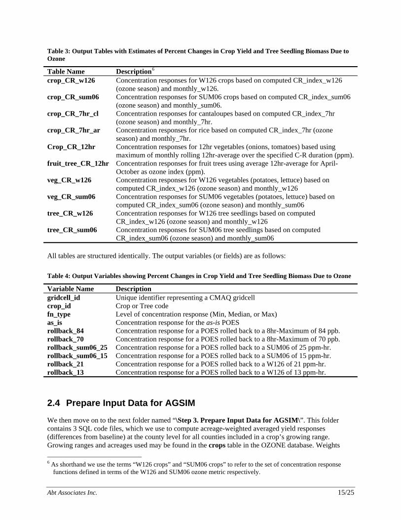
Table 3: Output Tables with Estimates of Percent Changes in Crop Yield and Tree Seedling Biomass Due to Ozone

Table Name Description6

crop_CR_w126 Concentration responses for W126 crops based on computed CR_index_w126 (ozone season) and monthly_w126.

crop_CR_sum06 Concentration responses for SUM06 crops based on computed CR_index_sum06 (ozone season) and monthly_sum06.

crop_CR_7hr_cl Concentration responses for cantaloupes based on computed CR_index_7hr (ozone season) and monthly_7hr.

crop_CR_7hr_ar Concentration responses for rice based on computed CR_index_7hr (ozone season) and monthly_7hr.

Crop_CR_12hr Concentration responses for 12hr vegetables (onions, tomatoes) based using maximum of monthly rolling 12hr-average over the specified C-R duration (ppm).

fruit_tree_CR_12hr Concentration responses for fruit trees using average 12hr-average for April-October as ozone index (ppm).

veg_CR_w126 Concentration responses for W126 vegetables (potatoes, lettuce) based on computed CR_index_w126 (ozone season) and monthly_w126

veg_CR_sum06 Concentration responses for SUM06 vegetables (potatoes, lettuce) based on computed CR_index_sum06 (ozone season) and monthly_sum06

tree_CR_w126 Concentration responses for W126 tree seedlings based on computed CR_index_w126 (ozone season) and monthly_w126

tree_CR_sum06 Concentration responses for SUM06 tree seedlings based on computed CR_index_sum06 (ozone season) and monthly_sum06

All tables are structured identically. The output variables (or fields) are as follows: Table 4: Output Variables showing Percent Changes in Crop Yield and Tree Seedling Biomass Due to Ozone

Variable Name Description gridcell_id Unique identifier representing a CMAQ gridcell crop_id Crop or Tree code fn_type Level of concentration response (Min, Median, or Max) as_is Concentration response for the as-is POES rollback_84 Concentration response for a POES rolled back to a 8hr-Maximum of 84 ppb. rollback_70 Concentration response for a POES rolled back to a 8hr-Maximum of 70 ppb. rollback_sum06_25 Concentration response for a POES rolled back to a SUM06 of 25 ppm-hr. rollback_sum06_15 Concentration response for a POES rolled back to a SUM06 of 15 ppm-hr. rollback_21 Concentration response for a POES rolled back to a W126 of 21 ppm-hr. rollback_13 Concentration response for a POES rolled back to a W126 of 13 ppm-hr.

2.4 Prepare Input Data for AGSIM

We then move on to the next folder named “\Step 3. Prepare Input Data for AGSIM\”. This folder contains 3 SQL code files, which we use to compute acreage-weighted averaged yield responses (differences from baseline) at the county level for all counties included in a crop’s growing range. Growing ranges and acreages used may be found in the crops table in the OZONE database. Weights 6 As shorthand we use the terms “W126 crops” and “SUM06 crops” to refer to the set of concentration response

functions defined in terms of the W126 and SUM06 ozone metric respectively.


were derived from NASS 2001 County Crop Data (planted acreage), and when NASS data was not available for a particular crop, we used the 2002 Census of Agriculture as a proxy (number of harvested farms). Run the files [Step 01. AgSim W126 (diff) over Range.sql] and [Step 01. AgSim SUM06 (diff) over Range.sql]. Note that the first file aggregates all W126 crops and vegetables, as well as all 7hr and 12hr crops, and produces one output table named tb_agsim_w126. The second file aggregates all SUM06 crops and vegetables, as well as 7hr and 12hr crops and produces one output table named tb_agsim_sum06. We then average county-level yield responses over each ERS region. Run the file named [Step 03. AgSim Agg.sql]. This file produces 2 output tables, tb_agsim_w126_agg and tb_agsim_sum06_agg, for the set of W126 and SUM06 crops respectively7. These two final tables are ready to be fed into the AGSIM Excel spreadsheet to estimate the welfare effects of the yield changes we estimated above.

2.5 Prepare Input Data for TREGRO

Similarly, in order to compute tree seedling biomass effects over the growing range of each tree species, two SQL code files in the folder “Step 4. Prepare Input Data for TREGRO” are used. Open and run [Step 01. Tree C-R SUM06 (diff) over Range.sql] and [Step 02. Tree C-R W126 (diff) over Range.sql]. Only run the second file if you are just interested in the results derived from the W126 C-R functions. Use the first file for the SUM06 C-R functions. As in Section 2.4 above, the two output tables, tree_CR_diff_w126_range and tree_CR_diff_sum06_range, show average concentration responses (differences from baseline) over the growing range of each tree species at the CMAQ gridcell level. These results were used to estimate the responses on total tree growth of two species, red maple and yellow (or tulip) poplar in two locations (Shenandoah National Park, VA, and Cranberry, NC) in the southern Appalachian Mountains for five O3 reduction scenarios. These simulations were carried out using the computable model, TREGRO. TREGRO is not publicly available, but more information is available on-line at http://eco.wiz.uni-kassel.de/model_db/mdb/tregro.html. The final results of the TREGRO analysis may be found in Chapter 7 of the Technical Report. For additional information regarding the parameters used in TREGRO, please contact David Weinstein, [email protected].

2.6 Prepare Input Data for ArcGIS Maps

In the next folder “Step 5. Prepare Input Data for Maps”, you will find one SQL code file, which is used to prepare input layers for the ArcGIS files used to produce crop yield and tree seedling biomass effects under the six air quality scenarios outlined in the Technical Report. Running the file named [Step 01. Maps.sql] produces estimated percent changes in yield (percent differences from baseline) at the gridcell level for Corn, Winter Wheat, Soybean, and Cotton, and estimated percent changes in tree

7 If you are running only one set of crops at a time (say using the C-R functions defined in terms of the W126 ozone

metric), then comment out the set of statements related to SUM06 crops, and vice-versa.



mailto:[email protected]


seedling biomass for Aspen, Ponderosa Pine, and Black Cherry over the whole continental U.S. The resulting tables are then exported to Microsoft Access or Excel, and may be used in ArcGIS. Please refer to the Readme document on the User’s Guide DVD at “\5 ArcGIS Files\readme.txt” for additional instructions and data sources to reproduce the maps presented in the Report. Briefly the procedure goes as follows:

1) From either SAS datasets and/or SQL tables, convert data to Microsoft Access format, and link grid latitude and longitude to crop and tree growing ranges at two resolutions: 12km (Eastern U.S.) and 36km (Western U.S.).

2) Import Access data to ESRI ArcGIS

3) Project data to NAD_1983_Lambert_Conformal_Conic

4) Convert feature class to raster with respect to the two spatial resolutions

5) Create a layout of the continental U.S., and mask those areas that do not fall within each species growing range

6) Save and export final layout

Carefully check the summary statistics produced by ArcGIS to make sure that maximum, minimum and average percent changes showed are computed over each species’ growing range (using the masked area), and not at the national level. Additional data layers were used to produce the final maps. These may be found under:

\basedata\ Outlines of counties, lakes, and countries \CropMask\ Masks for crop and tree growing ranges \SUM06_Crops\ Crop grids \SUM06_Trees\ Tree grids

The following file naming conventions were used for the grid files:

CR Corn CT Cotton SB Soybean WW Winter Wheat TAS Aspen TBC Black Cherry TPP Ponderosa Pine

For example:

w126is_cr12k Baseline for W126 Corn in the Eastern U.S. w126r70_cr12k Effect of 70 ppb rollback POES for W126 Corn in the Eastern U.S. w126r84_cr12k Effect of 84 ppb rollback POES for W126 in the Eastern U.S.

2.7 Compute Summary Statistics

The summary tables published in Chapter 5 of the Technical Report were produced from SAS code files available in the last folder named “Step 6. Generate Summary Tables”. The authors are making these


files available for reference purposes. Other statistical tools and methods may be used to produce comparative summaries. Each summary file produces maximum, minimum, mean, and median values, as well as top and bottom quartiles, and standard deviation. Note that you do not need to export the SQL tables produced in Sections 2.3, 2.4, and 2.5 above to SAS datasets, as you may create a SAS library referencing the OZONE SQL database. SAS will execute statements against the SQL database directly, which is a major time-saving feature. Proceed as follows:

1) Create a new ODBC data source to the OZONE database. Go to Start -> Control Panel -> Administrative Tools -> Data Sources (ODBC), and click the System DSN tab.

2) Click the Add button, and select SQL Native Client from the driver list.

3) In the next windows, enter the information shown in Figure 7 below.

4) Click OK 3 times and exit the ODBC Data Source Administrator.

5) Start SAS, and create a new library using the ODBC engine. Enter the information shown in Figure 8 below.

You may now execute the SAS files in folder “Step 6. Generate Summary Tables.”

Figure 7: Create a New ODBC Data Source Referencing the SQL “OZONE” Database

Figure 8: Create a New SAS Library Referencing the “OZONE” ODBC Data Source

Abt Associates Inc. 19


List of References Technical Report on Ozone Exposure, Risk, and Impact Assessments for Vegetation - http://www.epa.gov/ttn/naaqs/standards/ozone/s_o3_index.html

User’s Guide - http://www.epa.gov/ttn/naaqs/standards/ozone/s_o3_cr_td.html (see list of Technical Documents) and at the Fate, Exposure and Risk Analysis (FERA) website http://www.epa.gov/ttn/fera/risk_criteria.html (click Ozone Risk Analyses).

User’s Guide data and code files - http://www.epa.gov/ttn/naaqs/standards/ozone/s_o3_cr_td.html (see list of Technical Documents) and at the Fate, Exposure and Risk Analysis (FERA) website http://www.epa.gov/ttn/fera/risk_criteria.html (click Ozone Risk Analyses).

Abt Associates Inc (1995) Ozone NAAQS Benefits Analysis: California Crops, July 5, 1995.

AGSIM - http://oaspub.epa.gov/eims/eimsapi.dispdetail?deid=73813

CASTNet - http://www.epa.gov/airmarkets/emissions/raw/index.html

CMAQ - http://www.epa.gov/asmdnerl/CMAQ/cmaq_model.html

ESRI (2005) Annual World Temperature Zones, available on-line at http://www.geographynetwork.com/ESRI_Temp_Yr/

IPM Center (various), available on-line at http://nepmc.org/rese_profiles.cfm , http://www.ipmcenters.org/cropprofiles/ , http://www.ncpmc.org/profiles/ .

Lee, E. H.; Hogsett, W. E. (1996) Methodology for calculating inputs for ozone secondary standard benefits analysis: Part II. Report prepared for Office of Air Quality Planning and Standards, Air

Little, Elbert L. Jr. (1978) Digital Representations of Tree Species Range Maps from "Atlas of United States Trees", available on-line at http://esp.cr.usgs.gov/data/atlas/little/

Olszyk DM, Thompson CR, Poe MP. (1988) Crop loss assessment for California: modeling losses with different ozone standard scenarios. Environmental Pollution 53 (1-4), pp. 303-11.

SQL Server Express 2005 - http://msdn.microsoft.com/vstudio/express/sql/download/

Taylor, C.R., K.H. Reichelderfer and S.R. Johnson (1993). Agricultural Sector Models for the United States: Descriptions and Selected Policy Applications. Iowa State University Press, Ames, IA, 1993.

TREGRO - http://eco.wiz.uni-kassel.de/model_db/mdb/tregro.html.

USDA (1997), Usual Planting and Harvesting Dates for U.S. Field Crops, National Agricultural Statistics Service Agricultural Handbook Number 628, December 1997.

Weinstein, D. A., Gollands, B; and Retzlaff, W. A. (2001). The effects of ozone on a lower slope forest of the Great Smoky Mountain National Park: Simulations Linking an Individual Tree Model to a Stand Model. Forest Science 47 (1): 29-42.

Weinstein, D.A., P. B. Woodbury, B. Gollands, P. King, L. Lepak, D. Pendleton (2002). Assessment of Effects of Ozone on Forest Resources in the Southern Appalachian Mountains. Final Report. Southern Appalachian Mountain Initiative. Asheville, N.C. 1032 pgs. (47 p text, 70 figures, 31 tables, 11 appendices).

http://www.epa.gov/ttn/naaqs/standards/ozone/s_o3_index.html

http://www.epa.gov/ttn/naaqs/standards/ozone/s_o3_cr_td.html

http://www.epa.gov/ttn/fera/risk_criteria.html

http://www.epa.gov/ttn/naaqs/standards/ozone/s_o3_cr_td.html

http://www.epa.gov/ttn/fera/risk_criteria.html

http://oaspub.epa.gov/eims/eimsapi.dispdetail?deid=73813

http://www.epa.gov/airmarkets/emissions/raw/index.html

http://www.epa.gov/asmdnerl/CMAQ/cmaq_model.html




Glossary of Terms AGSIM A publicly available large-scale econometric simulation model of regional crop

and national livestock production in the U.S.

AQS Air Quality System

CASTNet Clean Air Status and Trends Network

CMAQ Community Multiscale Air Quality model

C-R Concentration-Response

CSV Comma-Separated Values (tabular text file)

ERS Economic Research Service

ESRI ArcGIS A set of Geographical Information Systems software used to map and visualize data

eVNA enhanced Voronoi Neighbor Averaging (interpolation method to combine monitored data with spatial scaling from CMAQ model outputs)

NASS National Agricultural Statistics Service

NetCDF Network Common Data Form

ODBC Open Database Connectivity

POES Potential Ozone Exposure Surface

SAS A statistical and data analysis language

SQL A relational database querying language

SUM06 An ozone exposure metric involving concentration weighting, defined as the sum of all hourly mean ozone concentrations equal to or greater than 60 ppb (refer to pp. 1.2 of the Technical Report for details).

TREGRO TREe GROwth: Response of Plants to Interacting Stresses

VNA/VNATool Voronoi Neighbor Averaging Tool used to interpolate data between gridcells

W126 An ozone exposure metric defined as a weighted sum of all ozone values observed between 8am and 8pm (refer to pp. 1.2 of the Technical Report for details).