user’s manual - 安世亚太 · ansys® mechanical user’s manual ... 3.11 estimate enclosed...
TRANSCRIPT

PE
P3⁄STRUCTURAL OPTIMIZATION (Vol. II)
GENESIS Topology for ANSYS® Mechanical
User’s Manual
GENESIS VERSION 14.0
February 2015
© VANDERPLAATS RESEARCH & DEVELOPMENT, INC.1767 SOUTH 8TH STREET SUITE 200
COLORADO SPRINGS, CO 80905Phone: (719) 473-4611 Fax: (719) 473-4638
http://www.vrand.comemail: [email protected]
安世
亚太
RA Global

PE
COPYRIGHT NOTICE
© Copyright, 1991-2015 by Vanderplaats Research & Development, Inc. All Rights Reserved, Worldwide. No part of this manual may be reproduced, transmitted, transcribed, stored in a retrieval system, or translated into any human or computer language, in any form or by any means, electronic, mechanical, magnetic, optical, chemical, manual, or otherwise, without the express written permission of Vanderplaats Research & Development, Inc., 1767 South 8th Street, Suite 200, Colorado Springs, CO 80905.
WARNING
This software and manual are both protected by U.S. copyright law (Title 17 United States Code). Unauthorized reproduction and/or sales may result in imprisonment of up to one year and fines of up to $10,000 (17 USC 506). Copyright infringers may also be subject to civil liability.
DISCLAIMER
Vanderplaats Research & Development, Inc. makes no representations or warranties with respect to the contents hereof and specifically disclaims any implied warranties of merchantability or fitness for any particular purpose. Further, Vanderplaats Research & Development, Inc. reserves the right to revise this publication and to make changes from time to time in the content hereof without obligation of Vanderplaats Research & Development, Inc. to notify any person or organization of such revision or change.
TRADEMARKS MENTIONED IN THIS MANUAL
GENESIS, DOT and DOC are trademarks of Vanderplaats Research & Development, Inc. ANSYS® is a registered trademark of ANSYS, Inc. Other products mentioned in this manual are trademarks of their respective developers or manufacturers.
P3⁄STRUCTURAL OPTIMIZATION (Vol. II)
安世
亚太
RA Global
PER
TABLE OF CONTENTS
CHAPTER 1 Introduction
1.1 GENESIS Topology for ANSYS Mechanical - - - - - - - - - - - 2
1.2 GENESIS and Topology Design Capabilities in GENESIS 3
1.3 Installation and Use of GTAM - - - - - - - - - - - - - - - - - - - - - - 4
CHAPTER 2 Structural Optimization Concepts
2.1 General Optimization - - - - - - - - - - - - - - - - - - - - - - - - - - - - 8
2.2 Special Methods for Structural Optimization - - - - - - - - - 132.2.1 Constraint Screening . . . . . . . . . . . . . . . . . . . . . . . . . . . . 152.2.2 Gradient Calculations . . . . . . . . . . . . . . . . . . . . . . . . . . . 162.2.3 Approximation Concepts . . . . . . . . . . . . . . . . . . . . . . . . . 182.2.4 Move Limits During Optimization . . . . . . . . . . . . . . . . . 202.2.5 Convergence to an Optimum . . . . . . . . . . . . . . . . . . . . . . 21
2.3 Topology Optimization - - - - - - - - - - - - - - - - - - - - - - - - - - 22
CHAPTER 3 Topology Optimization with GTAM
3.1 Overview - - - - - - - - - - - - - - - - - - - - - - - - - - - - - - - - - - - - - 24
3.2 Add GENESIS System to ANSYS Workbench Workflow 25
3.3 Topology Regions - - - - - - - - - - - - - - - - - - - - - - - - - - - - - - 263.3.1 Design Region Definition . . . . . . . . . . . . . . . . . . . . . . . . 273.3.2 Initial Mass Fraction . . . . . . . . . . . . . . . . . . . . . . . . . . . . 283.3.3 Fabrication Constraints . . . . . . . . . . . . . . . . . . . . . . . . . . 293.3.4 Power Rule. . . . . . . . . . . . . . . . . . . . . . . . . . . . . . . . . . . . 30
3.4 Topology Objectives - - - - - - - - - - - - - - - - - - - - - - - - - - - - 313.4.1 Response Type. . . . . . . . . . . . . . . . . . . . . . . . . . . . . . . . . 323.4.2 Objective Definition . . . . . . . . . . . . . . . . . . . . . . . . . . . . 40
3.5 Topology Constraints - - - - - - - - - - - - - - - - - - - - - - - - - - - 433.5.1 Response Type. . . . . . . . . . . . . . . . . . . . . . . . . . . . . . . . . 443.5.2 Constraint Bounds . . . . . . . . . . . . . . . . . . . . . . . . . . . . . . 45
3.6 Fabrication Constraints - - - - - - - - - - - - - - - - - - - - - - - - - 463.6.1 Element Based Topology vs. Geometry Based Topology 473.6.2 Mirror Symmetry . . . . . . . . . . . . . . . . . . . . . . . . . . . . . . . 483.6.3 Cyclic Symmetry . . . . . . . . . . . . . . . . . . . . . . . . . . . . . . . 49
安世
亚太
A Global
GENESIS April 2014 Design Manual 1
PER
3.6.4 Extrusion . . . . . . . . . . . . . . . . . . . . . . . . . . . . . . . . . . . . . 503.6.5 Filling. . . . . . . . . . . . . . . . . . . . . . . . . . . . . . . . . . . . . . . . 513.6.6 Sheet Forming . . . . . . . . . . . . . . . . . . . . . . . . . . . . . . . . . 533.6.7 Uniform . . . . . . . . . . . . . . . . . . . . . . . . . . . . . . . . . . . . . . 553.6.8 Radial Filling . . . . . . . . . . . . . . . . . . . . . . . . . . . . . . . . . . 573.6.9 Radial Spoke . . . . . . . . . . . . . . . . . . . . . . . . . . . . . . . . . . 593.6.10 Combining Fabrication Constraints . . . . . . . . . . . . . . . . . 603.6.11 List of All Fabrication Constraints . . . . . . . . . . . . . . . . . 623.6.12 Minimum Size Control . . . . . . . . . . . . . . . . . . . . . . . . . . 653.6.13 Maximum Size Control . . . . . . . . . . . . . . . . . . . . . . . . . . 67
3.7 Analysis Settings - - - - - - - - - - - - - - - - - - - - - - - - - - - - - - 683.7.1 Design Control . . . . . . . . . . . . . . . . . . . . . . . . . . . . . . . . . 693.7.2 Design Move Limits . . . . . . . . . . . . . . . . . . . . . . . . . . . . 703.7.3 Design Convergence . . . . . . . . . . . . . . . . . . . . . . . . . . . . 713.7.4 Design Methods . . . . . . . . . . . . . . . . . . . . . . . . . . . . . . . . 733.7.5 Analysis Control . . . . . . . . . . . . . . . . . . . . . . . . . . . . . . . 773.7.6 Design Output Control. . . . . . . . . . . . . . . . . . . . . . . . . . . 803.7.7 Analysis Output Control . . . . . . . . . . . . . . . . . . . . . . . . . 813.7.8 Post-Processing Control. . . . . . . . . . . . . . . . . . . . . . . . . . 833.7.9 Coarsened Surface . . . . . . . . . . . . . . . . . . . . . . . . . . . . . . 843.7.10 Modal/Buckling Analysis . . . . . . . . . . . . . . . . . . . . . . . . 853.7.11 Random Response . . . . . . . . . . . . . . . . . . . . . . . . . . . . . . 873.7.12 Random Output . . . . . . . . . . . . . . . . . . . . . . . . . . . . . . . . 883.7.13 Non-linear Contact. . . . . . . . . . . . . . . . . . . . . . . . . . . . . . 89
3.8 Files Generated during Optimization Process - - - - - - - - 903.8.1 Program Output (pname.out) . . . . . . . . . . . . . . . . . . . . . . 913.8.2 Analysis Post-Processing File(pname.pch or pname.op2) 923.8.3 Design Cycle History File (pname.HIS) . . . . . . . . . . . . . 933.8.4 Topology Density File (pnameDENSxx.HIS) . . . . . . . . . 94
3.9 Monitor Optimization Process - - - - - - - - - - - - - - - - - - - - 95
3.10 Post-Process Topology Result - - - - - - - - - - - - - - - - - - - - 96
3.11 Estimate Enclosed Volume for Isosurface - - - - - - - - - - - 97
3.12 Analyze Interpreted Topology Result - - - - - - - - - - - - - - - 98
3.13 Export Coarsened Surface - - - - - - - - - - - - - - - - - - - - - - 103
3.14 Additional Options - - - - - - - - - - - - - - - - - - - - - - - - - - - - 104
3.15 Recommendations - - - - - - - - - - - - - - - - - - - - - - - - - - - - 106
安世
亚太
A Global
2 Design Manual April 2014 GENESIS
PER
CHAPTER 4 Appendix
4.1 Appendix A: Features Support in Current Version - - - 108
4.2 Appendix B: Conversion Mapping - - - - - - - - - - - - - - - - 110安世
亚太
A Global
GENESIS April 2014 Design Manual 3
PER
安世
亚太
A Global
4 Design Manual April 2014 GENESIS
PE
P3⁄STRUCTURAL OPTIMIZATION (Vol. II)^
CHAPTER 1Introduction
o GENESIS Topology for ANSYS Mechanical
o GENESIS and Topology Design Capabilities in GENESIS
o Installation and Use of GTAM
安世
亚太
RA Global
GENESIS Topology for ANSYS Mechanical February 2015 User’s Manual 1
GENESIS Topology for ANSYS Mechanical
PE
1.1 GENESIS Topology for ANSYS MechanicalGENESIS Topology for ANSYS Mechanical (GTAM) is an integrated extension that adds topology optimization to the ANSYS environment. The extension is developed based on the ANSYS Customization Toolkit (ACT). By utilizing this toolkit, the users of the GTAM extension can access all the necessary information for defining the ANSYS analysis model and to convert it to the GENESIS input format automatically. The extension provides an easy-to-use interface which allows the user to setup topology optimization problems, post-process them and export the data within the ANSYS environment.
The basic steps to perform topology optimization in ANSYS include:
1. Add GENESIS analysis system to the ANSYS Workbench workflow by sharing the Model data with the existing analysis systems.
2. In ANSYS Mechanical, the user will add topology optimization data through the GENESIS Structural Optimization toolbar. This toolbar allows to:
Define Topology RegionsDefine Topology ObjectivesDefine Topology Constraints
3. Solve the Optimization Problem
In this step, GENESIS will be run in the background4. After the Topology optimization is solved, the user can post-process the results
which include:
Topology Element DensityTopology Density IsosurfaceDeformation, Stress, Strain, Strain Energy
5. As the last step, the user can export the optimized structure in a STL/IGES format.
安世
亚太
RA Global
2 User’s Manual February 2015 GENESIS Topology for ANSYS Mechanical
GENESIS and Topology Design Capabilities in GENESIS
PE
1.2 GENESIS and Topology Design Capabilities in GENESIS
GENESISGENESIS is a fully integrated finite element analysis and design optimization software package, written by leading experts in structural optimization.
Analysis is based on the finite element method for static, normal modes, direct and modal frequency analysis, random response analysis, heat transfer, and system buckling calculations.
Design is based on the advanced approximation concepts approach to find an optimum design efficiently and reliably. An approximate problem, generated using analysis and sensitivity information, is used for the actual optimization, which is performed by the well-established DOT or BIGDOT optimizers. When the optimum of the approximate problem has been found, a new finite element analysis is performed and the process is repeated until the solution has converged to the optimum.
Many design options are available for users including: shape, sizing, topography, topometry and topology.
Topology Design Capabilities in GENESISWith topology optimization, regions of the structure that have the least contribution to the overall stiffness or natural frequency are identified. This tells the user which regions should be removed from the structure to minimize the mass while having the least impact on the performance of the structure.
Parts or bodies are selected to be designed, and design variables are automatically created to control the stiffness and density of every element in that part or body. Isotropic, orthotropic and anisotropic material are all supported in topology design. Available responses include static displacements, strain energies, natural frequencies, buckling load factors, direct and modal displacements, velocities and accelerations; random root mean square displacement, velocities and accelerations, inertia responses and mass fraction. Special features for topology optimization include enforcing symmetries and/or fabrication constraints in the structure and a capability to reduce “checkerboard” like results. Mode tracking is available for both frequencies and buckling load factors.
Topology results, for post processing, are smoothed and surfaces representing density levels are output to aid the user to interpret topology optimization results.
安世
亚太
RA Global
GENESIS Topology for ANSYS Mechanical February 2015 User’s Manual 3
Installation and Use of GTAM
PE
1.3 Installation and Use of GTAMTo be able to run topology optimization in ANSYS, the user need to install both the GTAM extension and GENESIS.
Installing the ExtensionTo install the extension, the user needs to open ANSYS Workbench, and select Extensions --> Install extension from main menus. A dialog will pop up and the user need to browse to the location of the extension installation file with extension *.wbex.
Note that installation of the extension does not require administrative privileges. The extension will be installed in the user’s folder as below:
%appdata%\Ansys\{ver}\AdvancedAddinPackage\extensions\GenesisSolver\
where {ver} is related to the ANSYS version, for example v150 for ANSYS 15.0.
Enable the ExtensionBefore using the extension, the user needs to enable it. In ANSYS workbench, select Extensions --> Manage Extension from main menus. A dialog with a list of extensions will pop up. The user needs to check the checkbox for GenesisSolver to enable it. The user can also right click on GenesisSolver in the list and select Load as Default option. In this way, the user does not need to enable the extension every time when creating a new project.
It is strongly recommended to enable the extension before launching ANSYS Mechanical. Otherwise, there will be Invalid Solver Type error when solving the optimization.
Install GENESISTo be able to solve an optimization problem, GENESIS needs to be installed. GENESIS comes with a standard installer. The installation of GENESIS requieres administrative privileges.
GTAM Manuals and ExamplesThe installation of GTAM comes with a User’s Manual, and Examples Manual and corresponding example input files.
The user can find these manuals in the extension installation folder:
安世
亚太
RA Global
4 User’s Manual February 2015 GENESIS Topology for ANSYS Mechanical
Installation and Use of GTAM
PE
%appdata%\Ansys\{ver}\AdvancedAddinPackage\extensions\GenesisSolver\Help
The example input files for GTAM are in the Examples folder located in the extension installation folder:
%appdata%\Ansys\{ver}\AdvancedAddinPackage\extensions\GenesisSolver\Examples
where {ver} is related to the ANSYS version.
GENESIS Manuals and ExamplesIf the user is interested in other capabilities that are not currently supported in GTAM, he can reference to the GENESIS manuals and examples.
安世
亚太
RA Global
GENESIS Topology for ANSYS Mechanical February 2015 User’s Manual 5
Installation and Use of GTAM
PE
安世亚
太 RA Global
6 User’s Manual February 2015 GENESIS Topology for ANSYS Mechanical

PE
P3⁄STRUCTURAL OPTIMIZATION (Vol. II)
CHAPTER 2Structural Optimization Concepts
o General Optimization
o Special Methods for Structural Optimization
o Topology Optimization
安世
亚太
RA Global
GENESIS Topology for ANSYS Mechanical February 2015 Examples Manual 7
General Optimization
PE
2.1 General OptimizationNumerical optimization methods provide a uniquely general and versatile tool for design automation. Research and applications to structural design has been extensive and today these methods are finding their way into engineering offices. The methods that form the basis of most modern optimization were developed roughly 40 years ago, and the first application to nonlinear structural design was presented by Schmit in 1960. Much of the research in structural design since 1975 has been devoted to creating methods that are efficient for structural design problems where the analysis is expensive. This has resulted in various approximation methods that allow a high degree of efficiency while maintaining the essential features of the original problem.
Here, we will first define the general design task in terms of optimization. For structural optimization, we create an approximation to the original problem. This approximate problem is solved by the optimizer. The advantage is that it is not necessary to repeatedly call the finite element analysis during the actual optimization process. This greatly reduces the overall cost of structural design. In GENESIS, the DOT or BIGDOT optimization programs, developed by VR&D, are used to solve this optimization sub-problem.
In Section 2.2, some of the special techniques that have been devised to make structural optimization efficient will be discussed. It is these special techniques, that are contained in GENESIS, which make modern structural optimization efficient, relative to other applications.
Mathematical programming (the formal name for numerical optimization) provides a very general framework for scarce resource allocation, and the basic algorithms originate in the operations research community. Engineering applications include structural design, chemical process design, aerodynamic optimization, nonlinear control system design, mechanical component design, multi-discipline system design, and a variety of others. Because the statement of the numerical optimization problem is so close to the traditional statement of engineering design problems, the design tasks to which it can be applied are inexhaustible.
In the most general sense, numerical optimization solves the nonlinear, constrained problem: Find the set of design variables, contained in vector X, that will
Minimize:
(Eq. 2-1)
Subject to:
Xi i, 1 N,=
F X( )
安世
亚太
RA Global
8 Examples Manual February 2015 GENESIS Topology for ANSYS Mechanical
General Optimization
PE
(Eq. 2-2)
(Eq. 2-3)
Equation (Eq. 2-1) defines the objective function, which depends on the values of the design variables, X. (Eq. 2-2) is inequality constraints. Equality constraints of the form
could also be included. This is achieved by using two equal, but opposite in sign, inequality constraints. (Eq. 2-3) defines the region of search for the minimum. This provides limits on the individual design variables. The bounds defined by (Eq. 2-3) are referred to as side constraints. A clear understanding of the generality of this formulation makes the breadth of problems that can be addressed apparent. However, there are some important limitations to the present technology. First, it is assumed that the objective and constraint functions be continuous and smooth (continuously differentiable). Experience has shown this to be a more theoretical than practical requirement and this restriction is routinely violated in engineering design. A second requirement is that the design variables contained in X be continuous. In other words, we are not free to chose structural sections from a table. Also, we cannot treat the number of plies in a composite panel as a design variable, instead treating this as a continuous variable and rounding the result to an integer value. It is not that methods do not exist for dealing with discrete values of the variables. It is just that available methods lack the needed efficiency for widespread application to real engineering design. VR&D has developed software to deal with this case, and this is expected to be added in the future. Finally, even though there is no theoretical limit to the number of design variables contained in X, if we use optimization as a “black box” where we simply couple an analysis program to an optimization program, the number of design variables that can be considered is limited.
The general problem description given above is remarkably close to what we are accustomed to in engineering design. For example, assume we wish to determine the dimensions of a structural member that must satisfy a variety of design conditions. We normally wish to minimize mass, so the objective function, F(X), is the mass of the structure, which is a function of the sizing variables. However, we also must consider constraints on stresses, deflections, buckling and perhaps dynamic response limits. Assuming we model the structure as an assemblage of finite elements, we can calculate the stresses in the elements under each of the prescribed loading conditions. Then a typical stress limit may be stated as
(Eq. 2-4)
g j X( ) 0 j≤ 1 M,=
XiL Xi Xi
U i≤ ≤ 1 N,=
hk X( ) 0 k 1 L,= =
σL σijk σU≤ ≤
安世
亚太
RA Global
GENESIS Topology for ANSYS Mechanical February 2015 Examples Manual 9
General Optimization
PE
where i = element number, j = stress component and k = load condition. The compression and tensile stress limits are and , respectively (if we use a von Mises stress criterion, only would be used). While (Eq. 2-4) may initially appear to be different from the general optimization statement, it is easily converted to two equations of the form of (Eq. 2-2) as
(Eq. 2-5)
(Eq. 2-6)
Thus, the formal statement of the optimization task is essentially identical to the usual statement of the structural design task.
The denominator of (Eq. 2-5) and (Eq. 2-6) represent normalization factors. This is important since it places each constraint in an equal basis. For example, if the value of a stress constraint is -0.1 and the value of a displacement constraint is -0.1, this indicates that each constraint is within 10% of it’s allowable value. Without normalization, if a stress limit is 20,000, it would only be active (within a value of 0.1) if it’s value was 19,999.9. This is not meaningful since loads, material properties, and other physical parameters are not known to this accuracy.
It is often assumed that for optimization to be used, the functional relationships must be explicit. However, this is categorically untrue. It is only necessary to be able to evaluate the objective and constraint functions for proposed values of the design variables, X.
Using optimization as a design tool has several advantages. We can consider large numbers of variables relative to traditional methods. Also in a new design environment, we may not have a great deal of experience to guide us and so optimization often gives unexpected results which can greatly enhance the final product. Finally, one of the most powerful uses of optimization is to make early design trade-offs using simplified models. Here we can compare optimum designs instead of just comparing point designs.
On the other hand, optimization has some disadvantages to be aware of. The quality of the result is only as good as the underlying analysis. In the case of finite element analysis, we must remember that this is just a model of the real structure. Thus, if we ignore or forget an important constraint, optimization will take advantage of it, leading to a meaningless if not dangerous design. Also, there is a danger that by optimizing we will reduce the hidden factors of safety that now exist. In this context, we should re-think our use of optimization, using it as a design tool and not as a sole means to an end product.
σL σU
σU
g1 X( )σL σijk–
σL---------------------- 0≤=
g2 X( )σijk σU
–
σU----------------------- 0≤=
安世
亚太
RA Global
10 Examples Manual February 2015 GENESIS Topology for ANSYS Mechanical
General Optimization
PE
However, assuming we agree that optimization is useful, it is also important to know how these algorithms solve our design problems. Next, we briefly outline the basic optimization process, contained in the DOT program, to provide some insight into the numerical techniques used.
Most optimization algorithms do just what good designers do. They seek to find a perturbation to an existing design which will lead to an improvement. Thus, we seek a new design which is the old design plus a change, so
(Eq. 2-7)
Optimization algorithms use much the same formula, except it becomes a two step process. Here we update the design by the relationship
(Eq. 2-8)
where in (Eq. 2-8) is equivalent to in (Eq. 2-7). Here q is the iteration number, and numerous search directions (iterations) will be needed to reach the optimum. The engineer must provide an initial design, X0, but it need not be feasible; it may not satisfy the inequalities of (Eq. 2-2). Optimization will then determine a “Search Direction,” Sq that will improve the design. If the design is initially feasible, the search direction will reduce the objective function without violating the constraints. If the initial design is infeasible, the search direction will point toward the feasible region, even at the expense of increasing the objective function.
The next question is how far can we move in direction Sq before we must find a new search direction. This is called the “One-Dimensional Search” since we are just seeking the value of the scalar parameter, α, to improve the design as much as possible. If the design is feasible and we are reducing the objective function, we seek the value of α that will reduce F(X) as much as possible without driving any gj(X) positive or violating any bound (side constraint) on the components of X. If the design is initially infeasible, we seek the value of α that will overcome the constraint violations if possible, or will otherwise drive the design as near to the feasible region as possible. Note that this is precisely what a design engineer does under the same conditions. The difference is that optimization does it without the need to study many pages (or screens full) of computer output.
There are a wide variety of algorithms for determining the search direction, S, as well as for finding the value of α [1]. Determining α is conceptually a simple task. For example, we may pick several values of α and calculate the objective and constraint functions. Then we fit a polynomial curve to each function and determine the value that will minimize
Xnew Xold δX+=
Xq 1+ Xq αSq+=
αSq δX
安世
亚太
RA Global
GENESIS Topology for ANSYS Mechanical February 2015 Examples Manual 11
General Optimization
PE
F(X) or drive gj(X) to zero. Since we picked a search direction that will improve the design, we need only consider positive values of α. The minimum positive value of α from among all of these curve fits is the one we want. For further details of how the optimization problem is solved, the DOT user’s manual and reference [1] may be useful.
References
[1] Vanderplaats, G. N., Numerical Optimization Techniques for Engineering Design; with Applications, 3rd Ed., Vanderplaats Research & Development, 1999.
安世
亚太
RA Global
12 Examples Manual February 2015 GENESIS Topology for ANSYS Mechanical
Special Methods for Structural Optimization
PE
2.2 Special Methods for Structural Optimization
The state of the art in structural optimization is now reasonably well developed, relative to other applications. To provide an overview of the methods used in GENESIS, we will briefly outline several key ingredients to the structural optimization process. The key concept is that we solve the structural design problem without the large number of full finite element analyses that would be required if we simply coupled the FEM and Optimizers. It is important to understand, however, that even though we use approximations to achieve this, we retain the key features of the detailed analysis model. Thus, when we are finished, we will have the same design we would find if we were able to use the FEM analysis directly during optimization.
The basic optimization process contained in GENESIS is summarized in the following 10 steps.
1. Preprocess all input data and perform all non-repetitive operations (e.g., check data for correctness, create internal tables, set up the overall program flow).
2. Perform a detailed finite element analysis for the initial proposed design. Evaluate the design objective and all constraints.
3. Screen all constraints and retain those that are critical or near critical for further consideration. Typically only 2n to 3n constraints are retained, where n is the number of independent design variables.
4. Perform the sensitivity analysis (gradient computations) for the responses included in the objective function and the retained constraints.
5. Set up a high quality approximation to the original problem and solve it using the DOT or BIGDOT optimizer.
6. If no design improvement is possible, exit. This is called “soft convergence.”
7. Assuming the design variables have changed, update the analysis data and perform a detailed finite element analysis for this proposed design.
8. Evaluate the precise objective function and all constraints.
9. If the design is not improving and if all constraints are satisfied within a specified tolerance, exit. This is called “hard convergence.”
10. If progress is still being made toward the optimum, we say that one “design cycle” has been completed. We then repeat the process from step 3.
安世
亚太
RA Global
GENESIS Topology for ANSYS Mechanical February 2015 Examples Manual 13
Special Methods for Structural Optimization
PE
From this brief outline, it is seen that key components of the structural optimization process include the finite element analysis, constraint screening, sensitivity analysis, creation and solution of the approximate optimization problem, and judging when convergence has been achieved. It is assumed that the reader is familiar with the analysis process. The key parts of the design optimization process will be briefly discussed here to give a general understanding of the GENESIS design capabilities.安
世亚
太 RA Global
14 Examples Manual February 2015 GENESIS Topology for ANSYS Mechanical
Special Methods for Structural Optimization
PE
2.2.1 Constraint Screening
The first thing to note is that the design of real structures requires that a very large number of constraints must be satisfied. For example, assume we model a large structure with hundreds or even thousands of finite elements. We may recover the stress at several locations in each element under many different loading conditions. Assume we must limit the von Mises stress to be less than or equal a specified value, . Then, where i = the element number, j = the stress recovery location and k = the load condition. Clearly, the combination ijk can become very large, often over one million.
Because the optimization process requires gradients of the constraints, this could lead to a very costly design sensitivity process, far exceeding the cost of a single analysis. Therefore, we first “screen” the constraints and retain only those that are critical or potentially critical for the current design cycle. This is a two step process. First, we delete all constraints that are more negative than, say -0.3 (not within 30% of being critical). Next, we search the set of retained constraints and further delete all but a specified subset in a given region of the structure. The reason for this is that many nearby points in the structure may have approximately the same stress. However, only a few of these stress responses need to be retained to direct the design process.
σa σijk σa≤安世
亚太
RA Global
GENESIS Topology for ANSYS Mechanical February 2015 Examples Manual 15
Special Methods for Structural Optimization
PE
2.2.2 Gradient Calculations
Having identified the responses that will be retained during the current design cycle, the next step is to evaluate their gradients (sensitivities). The sensitivity of a static response, R, (e.g., stress, displacement, strain energy) with respect to a design variable, X, is determined by the chain rule of differentiation as follows:
(Eq. 2-9)
Using the governing global equilibrium equations ([K]U = F) the displacement sensitivities are determined as:
(Eq. 2-10)
where are referred to as pseudo-loads.
Therefore, the response sensitivity becomes:
(Eq. 2-11)
The direct method first calculates the displacement sensitivity and uses that to
calculate to form the response sensitivity. This method requires performing a
forward/back substitution (i.e., equivalent to solving a static loadcase) for each design variable.
The adjoint method first calculates and then dots that with the pseudo-load
to form the second part of the response derivative. Note that because K is symmetric, [K-
1]T = [K]-1. Therefore, this method require one forward/back substitution for each response. If the number of retained responses is smaller than the number of design variables, then the adjoint method should provide better performance.
By default, GENESIS will select the most efficient method automatically.
XddR
X∂∂R
U∂∂R
X∂∂U
+=
X∂∂U K[ ] 1–
X∂∂F
X∂∂K U–
⎩ ⎭⎨ ⎬⎧ ⎫
=
X∂∂F
X∂∂K U–
⎩ ⎭⎨ ⎬⎧ ⎫
XddR
X∂∂R
U∂∂R K[ ] 1–
X∂∂F
X∂∂K U–
⎩ ⎭⎨ ⎬⎧ ⎫
+=
X∂∂U
U∂∂R
X∂∂U
K 1–[ ]T
U∂∂R
⎩ ⎭⎨ ⎬⎧ ⎫
T
安世
亚太
RA Global
16 Examples Manual February 2015 GENESIS Topology for ANSYS Mechanical
Special Methods for Structural Optimization
PE
The pseudo-loads are formed on an element-by-element basis and assembled into a global vector. Where possible and efficient, an exact analytical process is used throughout the sensitivity calculations. In other cases, a semi-analytic technique is used, whereby the pseudo-load is calculated by finite difference, but the remainder of the sensitivity calculations are fully analytic.安
世亚
太 RA Global
GENESIS Topology for ANSYS Mechanical February 2015 Examples Manual 17

Special Methods for Structural Optimization
PE
2.2.3 Approximation Concepts
The key to efficiency of modern structural optimization lies in what is called “approximation concepts”. The simplest approximation method would be to create a linear approximation to the objective and constraint functions as:
(Eq. 2-12)
(Eq. 2-13)
These approximations are then sent to the optimizer to modify the design. In practice, move limits are imposed on the design variables so that they are not changed beyond the region of applicability of the approximation.
The repeated application of simple linearizations such as this is called “Sequential Linear Programming” and this has been used for nearly 30 years as a valid optimization strategy. However, in the special case of structural design, we are able to create approximations that are valid over a much wider range of the design variables.
Consider calculating the stress in a simple rod element, as . Now, if we linearize
the stress in terms of the design variable, A, we get
(Eq. 2-14)
The equation is quite nonlinear in A, and so the approximation is valid only for
small changes in A. Now consider using an “intermediate” variable, X=1/A, so . Linearizing with respect to X gives
(Eq. 2-15)
The equation is more linear in X and, in the special case of a statically determinate structure F is independent of X, so the approximation is precisely linear in X. The optimizer will now treat X as the design variable. When the approximate optimization is complete, we recover the cross-sectional areas as A=1/X.
F̃ X( ) F X0( ) ∇F X0( ) X X0–{ }⋅+=
g̃j X( ) gj X0( ) ∇gj X0( ) X X0–( ) j⋅+ 1 M,= =
σ F A( )A
------------=
σ̃ σ0 σ∂A∂
-------δA+ σ0 1
A0------- F0∂
A∂--------- σ0
–⎩ ⎭⎨ ⎬⎧ ⎫
δA+= =
σ FA----=
σ FX=( )x
σ̃ σ0 σ∂X∂
-------δX+ σ0F0 F0∂
X∂---------X0
+⎩ ⎭⎨ ⎬⎧ ⎫
δX+= =
σ F X( ) X⋅=
安世
亚太
RA Global
18 Examples Manual February 2015 GENESIS Topology for ANSYS Mechanical
Special Methods for Structural Optimization
PE
As another example, consider a rectangular beam element, with the width, B, and height, H, as design variables. We can treat the section properties (e.g., A, I, J) as intermediate variables and calculate the approximate stresses and displacements in terms of these. Then, when the optimizer requires the stress or displacement values, we first calculate the section properties as explicit functions of the design variables, B and H, and recover the responses from the linearized quantities. In this fashion, we retain considerable nonlinearity contained in the design variable to section property relationships.
Now take this process one step further by considering intermediate responses. Here, for stress constraints in a rod, we approximate the force, F, instead of stress in the rod. When stress is needed, we first calculate the approximate force in the element as
(Eq. 2-16)
Then we recover the stress as . This can be shown to be a higher quality
approximation than found by using the reciprocal variable, X, and a much higher quality approximation than found by direct linearization.
GENESIS uses these approximations, as well as a variety of others, to improve the overall efficiency and reliability of the structural design process. The key concept is that we are free to restate the optimization problem in whatever form is best, as long as we retain the important mathematical features of the original problem. By using high quality approximations, we use only the approximated functions during optimization. In this way, we avoid the large number of finite element analyses normally needed for optimization using numerical search methods.
F̃ F0 F∂A∂
-------δA+=
σ F̃A----≈
安世
亚太
RA Global
GENESIS Topology for ANSYS Mechanical February 2015 Examples Manual 19
Special Methods for Structural Optimization
PE
2.2.4 Move Limits During Optimization
Even though GENESIS uses very high quality approximations to drive the design process, they are still not a precise representation of the model analyzed by the FEM model. Therefore, it is important to limit the design changes during any single design cycle. To do this, “move limits” are used, being the amount by which the design variables can change before it is considered necessary to perform a detailed analysis of the new proposed design. Additionally, because GENESIS uses intermediate variables, move limits are imposed on the element section properties, since these are used in the Taylor series expansions. Typically, the design variables and section properties are allowed to change by 50% during a design cycle. This is roughly 4-5 times the design changes that could be allowed if simple linearization methods were used. In practice, the move limits are not active as the optimization process converges, but they are important in the early design cycles to properly direct the design process.
安世
亚太
RA Global
20 Examples Manual February 2015 GENESIS Topology for ANSYS Mechanical
Special Methods for Structural Optimization
PE
2.2.5 Convergence to an Optimum
Because the optimization process is iterative, it is necessary to judge when the process is complete and should be stopped. GENESIS uses a variety of mechanisms to detect convergence. The first and most obvious is that the optimization process will automatically be terminated after a user defined number of design cycles. The default limit is ten design cycles, and this will normally produce a high quality optimum, assuming a reasonable initial design was provided.
Beyond this, GENESIS considers both “Soft Convergence” and “Hard Convergence” tests. Soft convergence is defined as the case where no further progress can be made (i.e., the design variables do not change). Since the design variables did not change, it is considered unnecessary to perform an additional detailed analysis and repeat the process. Hard convergence occurs when two consecutive design cycles do not improve the optimum appreciably, even though significant changes in the design variables are occurring. In this case, since the design variables did change, a detailed analysis is required to insure the quality of the proposed design.
On contact analysis optimization problems, if soft or hard converge occurs on a design cycle where no full contact analysis was performed, the program will not stop and it will issue a warning message.
安世
亚太
RA Global
GENESIS Topology for ANSYS Mechanical February 2015 Examples Manual 21
Topology Optimization
PE
2.3 Topology Optimization
Topology optimization is used to find the optimal distribution of material in a given package space. Unlike shape and sizing optimization, topology optimization does not require an initial design. Typically, the design starts with a block of material formed by a large number of finite elements and the topology optimization will eliminate the unnecessary elements from the block.
Topology optimization has a limited number of responses associated with it. These responses are primarily used to create a stiff and light structure.
Topology optimization is normally used by design engineers to perform conceptual designs. After the topology optimization is finished, shape and/or sizing optimization can be performed to refine the solution. To implement the shape/sizing optimization the user has to re-build the analysis model by removing the elements that TOPOLOGY has indicated to be unnecessary. Topology results in STL or IGES format are typically used to facilitate the redesign process.
In GENESIS, topology optimization works by creating design variables associated with the Young’s modulus and density of each element in the package space. The value of the design variable ranges between 0.0 and 1.0, where 1.0 indicates that the element has its normal stiffness and mass, and 0.0 indicates that the element has no stiffness or mass. Several different relationships between the stiffness and density of an element are available.
Topology optimization can be used with static, non-linear contact, eigenvalue, buckling, dynamic and random load cases. Currently, it cannot be used with heat transfer load cases. The relevant results are the displacements, strain energy, natural frequency, buckling load factors, modal/direct/random displacement velocities and acceleration responses. The remaining analysis results (e.g., STRESS, STRAIN and FORCES) should only be used as reference solutions because they are theoretically valid only in the limits of the design variables (0.0 or 1.0). The reason for this is obvious: material properties are not really variable. This is just a method to identify which material to keep (design variable close to 1.0) and which material to discard (design variable close to 0.0).
Geometric responses such as moment of inertia, center of gravity and mass fraction can also be used in topology optimization.
Fabrication requirements such as minimum/maximum member size, castability, extrusion, stamping and symmetries can be imposed if necessary.
安世
亚太
RA Global
22 Examples Manual February 2015 GENESIS Topology for ANSYS Mechanical
PE
P3⁄STRUCTURAL OPTIMIZATION (Vol. II)
CHAPTER 3Topology Optimization with GTAM
o Overview
o Add GENESIS System to ANSYS Workbench Workflow
o Topology Regions
o Topology Objectives
o Topology Constraints
o Fabrication Constraints
o Analysis Settings
o Files Generated during Optimization Process
o Monitor Optimization Process
o Post-Process Topology Result
o Estimate Enclosed Volume for Isosurface
o Analyze Interpreted Topology Result
o Export Coarsened Surface
o Additional Options
o Recommendations
安世
亚太
RA Global
GENESIS Topology for ANSYS Mechanical February 2015 Examples Manual 23
Overview
PE
3.1 OverviewThe basic steps to perform topology optimization in ANSYS include:
1. Add GENESIS system to an ANSYS Workbench workflow by sharing the Model data with the existing analysis systems.
2. In ANSYS Mechanical, the user can add topology optimization data through the GENESIS Structural Optimization toolbar. Using this toolbar the user can:
Define Topology RegionsDefine Topology ObjectivesDefine Topology Constraints
3. Solve the Optimization
GENESIS will be run in the background4. After the Topology optimization is solved, the user can post-process the results. This
includes:
Topology Element DensityTopology Density IsosurfaceDeformation, Stress, Strain, Strain Energy
5. As the last step, the user can export the optimized structure in a STL/IGES format.
In the following chapters, each of this steps and corresponding information will be described with more details.
安世
亚太
RA Global
24 Examples Manual February 2015 GENESIS Topology for ANSYS Mechanical
Add GENESIS System to ANSYS Workbench Workflow
PE
3.2 Add GENESIS System to ANSYS Workbench WorkflowThe first step to setup a topology optimization in ANSYS is to add a GENESIS system to an existing workflow and share the Model data with other analysis systems (Figure 3-1). It is required that all the analysis systems that are needed to be designed with GENESIS share their Model data with GENESIS. By sharing the Model data, GENESIS can access all the information defining the ANSYS model such as material properties, mesh, connections, load and boundary conditions for each analysis system. GENESIS will treat each analysis system as one loadcase if the analysis system is single-step analysis. If the analysis system is multiple-step analysis, then each step will be converted to a separate loadcase.
Figure 3-1Add GENESIS to ANSYS Workbench workflow
Please note that the order of analysis systems in the workflow does not matter if they are not sharing any solution data. The position of the GENESIS system does not matter either. Basically, all the analysis systems that share the Model data with GENESIS will be parsed and converted to GENESIS loadcases.
安世
亚太
RA Global
GENESIS Topology for ANSYS Mechanical February 2015 Examples Manual 25
Topology Regions
PE
3.3 Topology RegionsThe Topology Regions ( ) object is used to define the topology design region where the optimization process will decide which element will be either kept or eliminated. When defining the topology regions, optionally, the user can impose certain Topology Objectives for the region.
Figure 3-2Details of Topology Regions
安世
亚太
RA Global
26 Examples Manual February 2015 GENESIS Topology for ANSYS Mechanical
Topology Regions
PE
3.3.1 Design Region DefinitionDesign Region is to specify the designable region for topology optimization. Only bodies or parts can be selected as topology designed region. Multiple bodies or parts can be selected and defined as one design region.
Any parts or bodies that are not selected in a design region will not be designed/changed by topology optimization.
Frozen RegionOptionally, the user can specify surfaces or edges on a topology designed region as Frozen Region. If a surface or an edge is defined as frozen, the elements that have a node on this surface/edge will be excluded from topology optimization and kept intact.
Frozen surface or edge can only be selected from a designable region.
安世
亚太
RA Global
GENESIS Topology for ANSYS Mechanical February 2015 Examples Manual 27
Topology Regions
PE
3.3.2 Initial Mass FractionMass Fraction is the quotient between the mass calculated using the topology density variable and the mass calculated using the full density (topology density variable =1.0). The topology density variable is a design variable that the program creates internally and that can take values between 0.0 and 1.0.
Note: Elements associated to the design variables with a value of 0.0 are normally discarded while elements associated with design variables with a value of 1.0 are normally kept.
Initial Mass Fraction is the percentage of material that the user chooses to start the optimization with. It is recommended to set Initial Mass Fraction to the final value that the user would like to achieve. Commonly used value for initial mass fraction are 0.3 or 0.5. The maximum value for initial mass fraction is 1.0.
安世
亚太
RA Global
28 Examples Manual February 2015 GENESIS Topology for ANSYS Mechanical
Topology Regions
PE
3.3.3 Fabrication ConstraintsFabrication Constraints are used to enforce manufacturing requirements. Available fabrication constraints include: Mirror Symmetry, Cyclic Symmetry, Extrusion, Filling, Sheet Forming, Uniform, Radial Filling, Radial Spoke. Up to three manufacture constraints can be imposed on the given topology region (Combining Fabrication Constraints). The user can also specify desired Minimum Member Size or Maximum Member Size for topology generated components. Optionally, the user can specify a Spread Fraction to get a smoother topology result. Details are discussed in section 3.6 Fabrication Constraints
安世
亚太
RA Global
GENESIS Topology for ANSYS Mechanical February 2015 Examples Manual 29
Topology Regions
PE
3.3.4 Power Rule
Relationships Between Design Variables and Material PropertiesGENESIS uses the density based method to solve the topology optimization problem. This method requires the creation of relationships between the design variables and the materials.
The typical relationship (POWER rule, which is the GENESIS default) is:
(Eq. 3-1)
(Eq. 3-2)
(Eq. 3-3)
where
E(X) - Young’s modulus
E0 - Initial Young’s modulus (this is the value in MAT1)
ρ(X) - Density
ρ0 - Initial density (this is the value in MAT1)
X - Topology design variables which represents the volume fraction (fraction of solid material)
TMIN - Minimum value of the topology design variable.
RV1 - Real value supplied by user (Typically: 2.0 < RV1 < 3.0)
RV2 - Real parameter representing , where EMIN is the minimum value Young’s modulus is
allowed to take. (0.0 < RV2 < 1.0, Typically RV2=10-6 which is the Default)
These equations create a heuristic relationship between the Young’s modulus and the density. In theory the relationships are true only if the design variables are 0.0 or 1.0. If a design variables is 1.0 then what this means is that its corresponding element is needed. If the design variable is 0.0 then its corresponding element is not needed and therefore it can be taken out of the model.
E X( ) E0RV2 E0 1 RV2–( )XRV1+=
ρ X( ) ρ0X=
TMIN X 1.0≤ ≤
EMINE0
------------
安世
亚太
RA Global
30 Examples Manual February 2015 GENESIS Topology for ANSYS Mechanical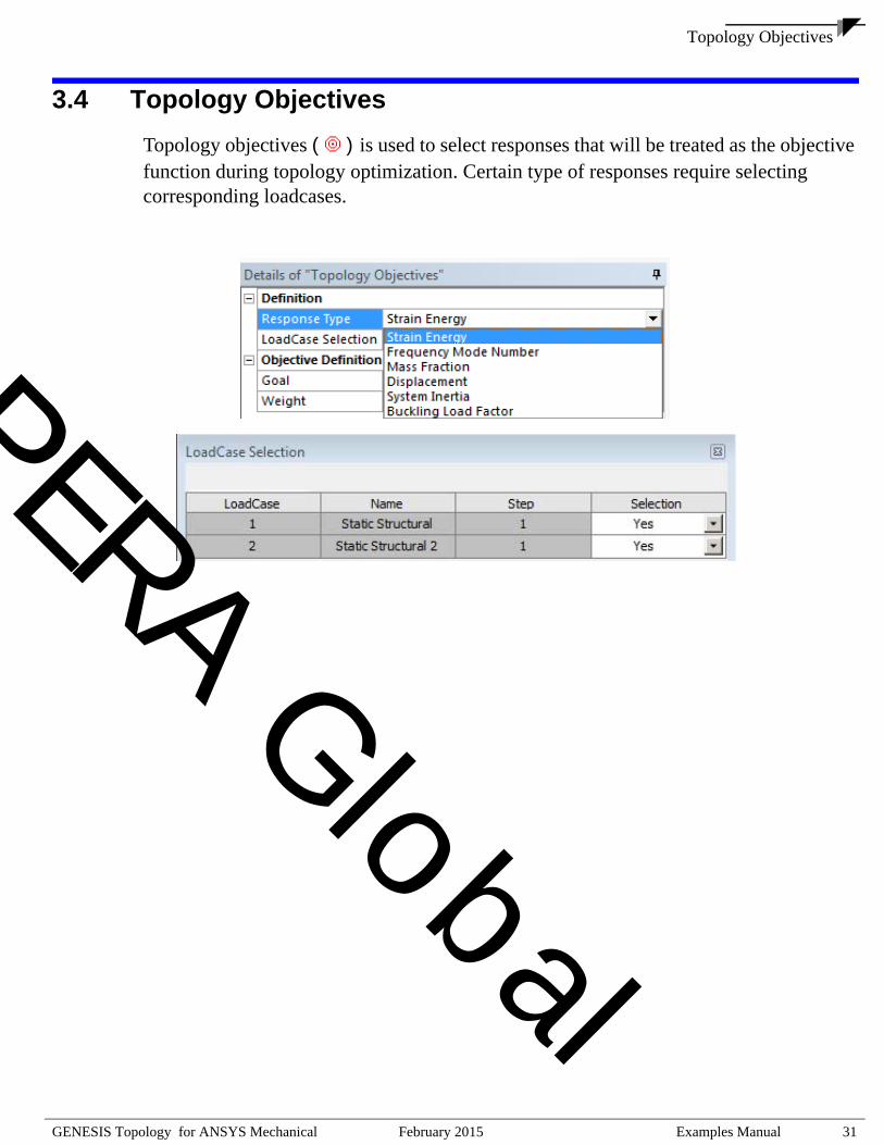
Topology Objectives
PE
3.4 Topology ObjectivesTopology objectives ( ) is used to select responses that will be treated as the objective function during topology optimization. Certain type of responses require selecting corresponding loadcases.安
世亚
太 RA Global
GENESIS Topology for ANSYS Mechanical February 2015 Examples Manual 31

Topology Objectives
PE
3.4.1 Response TypeIn current version of GENESIS Topology for ANSYS Mechanical, the supported response types are described in following sections.
Strain EnergyStrain Energy of the whole model. Corresponding loadcases need to be selected for this type of response. The response is a single scalar value for each loadcase.
Note: For most common problems, the smaller the strain energy, the stiffer the structure. In less common problems such as problems with enforced displacements the opposite is true, the larger the strain energy, the stiffer the structure.
Mass FractionFractional mass associated with the selected design region or all design regions. The response value is a single scalar value.
Region• Selected Groups
This option is to define the mass fraction to be associated with selected topology designed regions.
• All Design GroupsThis option is to define mass fraction to be associated with all topology designed regions.
DisplacementStatic displacement of the given grid/grids. Corresponding loadcases need to be selected for this type of response.
Geometry SelectionThe scopable entity includes node, vertex, edge, or surface. If more than one node is selected or the selected geometry entity contains more than one node, then the response is a vector for each loadcase.
Coordinate System
安世
亚太
RA Global
32 Examples Manual February 2015 GENESIS Topology for ANSYS Mechanical
Topology Objectives
PE
The user can define a Coordinate System which the displacement refers to.
ComponentsAvailable options are:
• Magnitude• Translation X• Translation Y• Translation Z• Rotation X• Rotation Y• Rotation Z
Relative DisplacementStatic relative displacement between the given reference grid and primary grid/grids. Corresponding loadcases need to be selected for this type of response.
Primary Grid SelectionThe scopable entity for Primary Grid includes node, vertex, edge, or surface. If more than one node is selected or the selected geometry entity contains more than one node, then the response is a vector for each loadcase.
Reference Grid SelectionThe scopable entity for Reference Grid includes node or vertex. Only one node/vertex is allowed to be selected as reference grid.
The relative displacement is calculated as displacement of the primary grid subtracts displacement of the reference grid.
Coordinate SystemThe user can define a Coordinate System which the displacement refers to.
ComponentsAvailable options are:
• Magnitude
安世
亚太
RA Global
GENESIS Topology for ANSYS Mechanical February 2015 Examples Manual 33
Topology Objectives
PE
• Translation X• Translation Y• Translation Z• Rotation X• Rotation Y• Rotation Z
Frequency Mode NumberNatural frequency associated with a given mode number for modal analysis. A corresponding loadcase is needed for selecting this type of response. The response is a single scalar value for each loadcase.
Mode NumberThe mode number of the natural frequency.
During topology optimization, due to the change of the material distribution, the mode shape can change shifting the mode number. Mode Tracking can be used in this case to track the given mode during optimization.
System InertiaSystem inertia of the model.
Components• Ixx at center of gravity• Iyy at center of gravity• Izz at center of gravity• Ixy at center of gravity• Iyz at center of gravity• Izx at center of gravity• Principal 1 at center of gravity• Principal 2 at center of gravity• Principal 3 at center of gravity• Ixx at grdpnt• Iyy at grdpnt• Izz at grdpnt
安世
亚太
RA Global
34 Examples Manual February 2015 GENESIS Topology for ANSYS Mechanical
Topology Objectives
PE
• Ixy at grdpnt• Iyz at grdpnt• Izx at grdpnt• Principal 1 at grdpnt• Principal 2 at grdpnt• Principal 3 at grdpnt• Y center of gravity with respect to grid• Z center of gravity with respect to grid• X center of gravity with respect to grid
Grid SelectionTo define the system inertia be calculated with respect to a given node. The scopable entity is vertex or node. Only one grid or vertex should be selected.
Buckling Load FactorBuckling load factor associated to a given mode number. A corresponding loadcases is needed for this type of response. The response is a single scalar value for each loadcase.
Mode NumberThe mode number of buckling load factor.
Dynamic DisplacementDynamic displacement calculated from a frequency response.
Response From• Direct
The response is calculated from direct harmonic analysis. The response is a vector with displacement value at each loading frequency value for a given node.
• ModalThe response is calculated from modal harmonic analysis. The response is a vector with displacement value at each loading frequency value for a given node.
• Random RMS
安世
亚太
RA Global
GENESIS Topology for ANSYS Mechanical February 2015 Examples Manual 35
Topology Objectives
PE
The Root Mean Square (RMS) of a random response quantity. The response is calculated from random analysis. The response is a single scalar value for a given node.
• Random PSDOutput for the Power Spectral Density (PSD) functions evaluated at each frequency value. The response is calculated from random analysis. The response is a vector for a given node.
Geometry SelectionThe scopable entity includes node, vertex, edge, or surface. If more than one node is selected or the selected geometry entity contains more than one node:
• for response from Direct or Modal, the response value is a vector with displacement value at each frequency for each selected node.
• for response from Random RMS, the response value is a vector with RMS value for each selected node.
• for response from Random PSD, the response value is a vector with PSD output at each frequency for each selected node.
Coordinate SystemThe user can define a Coordinate System which the displacement refers to.
ComponentsAvailable options are:
• Translation X• Translation Y• Translation Z• Rotation X• Rotation Y• Rotation Z
Dynamic VelocityDynamic velocity calculated from frequency response.
Response From
安世
亚太
RA Global
36 Examples Manual February 2015 GENESIS Topology for ANSYS Mechanical
Topology Objectives
PE
• DirectThe response is calculated from direct harmonic analysis. The response is a vector with velocity value at each loading frequency value for a given node.
• ModalThe response is calculated from modal harmonic analysis. The response is a vector with velocity value at each loading frequency value for a given node.
• Random RMSThe Root Mean Square (RMS) of a random response quantity. The response is calculated from random analysis. The response is a single scalar value for a given node.
• Random PSDOutput for the Power Spectral Density (PSD) functions evaluated at each frequency value. The response is calculated from random analysis. The response is a vector for a given node.
Geometry SelectionThe scopable entity includes node, vertex, edge, or surface. If more than one node is selected or the selected geometry entity contains more than one node:
• for response from Direct or Modal, the response value is a vector with velocity value at each frequency for each selected node.
• for response from Random RMS, the response value is a vector with RMS value for each selected node.
• for response from Random PSD, the response value is a vector with PSD output at each frequency for each selected node.
Coordinate SystemThe user can define a Coordinate System which the displacement refers to.
ComponentsAvailable options are:
• Translation X• Translation Y• Translation Z• Rotation X• Rotation Y
安世
亚太
RA Global
GENESIS Topology for ANSYS Mechanical February 2015 Examples Manual 37
Topology Objectives
PE
• Rotation Z
Dynamic AccelerationDynamic acceleration calculated from frequency response.
Response From• Direct
The response is calculated from direct harmonic analysis. The response is a vector with acceleration value at each loading frequency value for a given node.
• ModalThe response is calculated from modal harmonic analysis. The response is a vector with acceleration value at each loading frequency value for a given node.
• Random RMSThe Root Mean Square (RMS) of a random response quantity. The response is calculated from random analysis. The response is a single scalar value for a given node.
• Random PSDOutput for the Power Spectral Density (PSD) functions evaluated at each frequency value. The response is calculated from random analysis. The response is a vector for a given node.
Geometry SelectionThe scopable entity includes node, vertex, edge, or surface. If more than one node is selected or the selected geometry entity contains more than one node:
• for response from Direct or Modal, the response value is a vector with acceleration value at each frequency for each selected node.
• for response from Random RMS, the response value is a vector with RMS value for each selected node.
• for response from Random PSD, the response value is a vector with PSD output at each frequency for each selected node.
Coordinate SystemThe user can define a Coordinate System which the displacement refers to.
Components
安世
亚太
RA Global
38 Examples Manual February 2015 GENESIS Topology for ANSYS Mechanical
Topology Objectives
PE
Available options are:
• Translation X• Translation Y• Translation Z• Rotation X• Rotation Y• Rotation Z
Other ResponsesThe Design Studio for GENESIS software could be optionally used for additional response types.
安世
亚太
RA Global
GENESIS Topology for ANSYS Mechanical February 2015 Examples Manual 39
Topology Objectives
PE
3.4.2 Objective Definition
Objective with Multiple Response ValuesBased on the type of responses, associated geometry/node selection, and loadcase selection, the defined objective can contain one or multiple response values. In the following cases, the defined objective contains multiple values:
• The response is a vector• The response is a scalar but there are multiple nodes selected (or scoped geometry
contains more than one node)• The response is a scalar but there are multiple load cases selected
In those cases, the program will convert multiple objective values into a single objective value.
GoalThe user must select minimize, maximize, or min-max the objective as the goal.
Minimize or Maximize• Minimize
Minimize the selected response.• Maximize
Maximize the selected response.
If the defined objective contains multiple values, or there are multiple objectives defined, those values or objectives will be converted as a single objective value using weighted sum method. Topology Index (TINDEXM) controls how those response values are converted. The options are:
• Normalized ReciprocalResponse are normalized. For a response to be minimized, GENESIS uses the direct contribution of the normalized response. For a response to be maximized, GENESIS uses the reciprocal contribution of the normalized response.
• Normalized DirectResponse are normalized. For a response to be minimized, GENESIS uses the direct contribution of the normalized response. For a response to be maximized, GENESIS uses the direct contribution of the normalized response with negative weighting factor.
安世
亚太
RA Global
40 Examples Manual February 2015 GENESIS Topology for ANSYS Mechanical
Topology Objectives
PE
• ReciprocalFor a response to be minimized, GENESIS uses the direct contribution of this response. For a response to be maximized, GENESIS uses the reciprocal contribution of this response.
• DirectFor a response to be minimized, GENESIS uses the direct contribution of this response. For a response to be maximized, GENESIS uses the direct contribution of this response with negative weighting factor.
By default, Normalized Reciprocal is used.
Min-MaxMin-max is usually selected to minimize the maximum or peak value of a vector response such as dynamic displacement, velocity or acceleration for frequency response. Internally, the Beta method is used to solve the min-max optimization problem.
We introduce an artificial design variable called Beta and additional constraint equations using this Beta value. Internally, the objective function is set to minimize Beta and the scaled dynamic responses are constrained to be less than Beta. If the value of Beta is reduced, the peak (maximum) value of the dynamic response must reduce in order to satisfy the Beta constraints. This method is called the Beta method and is commonly used to solve the min-max (minimizing the maximum response) problem.
The following optimization problem will be created internally:
Objective:
Minimize Beta
Subject to:
(Dynamic Response)/(Scale Factor)-Beta < 0.0Other user defined constraints
Where Scale Factor is usually the peak response value of the nominal design. The user can specify this value in Initial Peak Response Value field.
WeightThe weighting factor for the given objective.
安世
亚太
RA Global
GENESIS Topology for ANSYS Mechanical February 2015 Examples Manual 41
Topology Objectives
PE
ShiftedIf this option is selected, the objective will be:
Objective=Response_Value+Shifted_Response_Value安世
亚太
RA Global
42 Examples Manual February 2015 GENESIS Topology for ANSYS Mechanical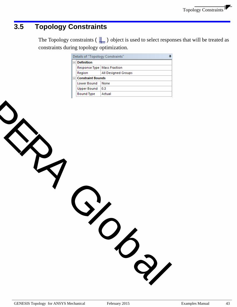
Topology Constraints
PE
3.5 Topology Constraints
The Topology constraints ( ) object is used to select responses that will be treated as constraints during topology optimization.安
世亚
太 RA Global
GENESIS Topology for ANSYS Mechanical February 2015 Examples Manual 43

Topology Constraints
PE
3.5.1 Response TypeThe same type of responses supported in Topology Objective are also available in Topology Constraints. Please refer to 3.4.1 Response Type for more details.
安世
亚太
RA Global
44 Examples Manual February 2015 GENESIS Topology for ANSYS Mechanical
Topology Constraints
PE
3.5.2 Constraint Bounds
BoundsTo define the lower and upper bounds for this constraint.
Similar as discussed in Topology Objective ( Objective with Multiple Response Values), the defined constraint can contain multiple response values. If the defined constraint contains multiple values, the constraint bounds will be applied on each response value.
Bound TypeActual means the given value will be used as constraint bounds directly.
Scale of Initial will use percentage of initial response value as constraint bounds.
安世
亚太
RA Global
GENESIS Topology for ANSYS Mechanical February 2015 Examples Manual 45
Fabrication Constraints
PE
3.6 Fabrication ConstraintsFabrication Constraints are used to enforce manufacturing requirements. Available fabrication constraints include: Mirror Symmetry, Cyclic Symmetry, Extrusion, Filling, Sheet Forming, Uniform, Radial Filling, Radial Spoke. Up to three manufacture constraints can be imposed on the given topology region (Combining Fabrication Constraints). The user can also specify desired Minimum Member Size or Maximum Member Size for topology generated components. Optionally, the user can specify a Spread Fraction to get a smoother topology result.
Coordinate SystemThe user must specify a Coordinate System which the fabrication constraints refer to.
安世
亚太
RA Global
46 Examples Manual February 2015 GENESIS Topology for ANSYS Mechanical
Fabrication Constraints
PE
3.6.1 Element Based Topology vs. Geometry Based TopologyElement based topology uses design variables that are associated with each element in the designable region. Geometry based topology uses design variables that are mesh independent. Geometry based method requires specifying a minimum member size. Using a larger value for minimum member size results in fewer design variables. Geometry based method is recommended or required in the following cases:
• Symmetry on a mesh that are not symmetric• Cyclic symmetry on a mesh that are not cyclic symmetric• Extrusion on a mesh that is not uniform along the given extrusion direction (i.e. solid
elements created by extruding a 2-D mesh) • Filling constraints• Sheet forming constraints• Uniform in parallel planes on a mesh that is not uniform in planes parallel to the given
plane (i.e., solid elements created by extruding a 2-D mesh).• Radial filling constraints• Radial spoke constraints
When there is a minimum member size specified, geometry based method is used by the program. Otherwise, the element based method is used.
安世
亚太
RA Global
GENESIS Topology for ANSYS Mechanical February 2015 Examples Manual 47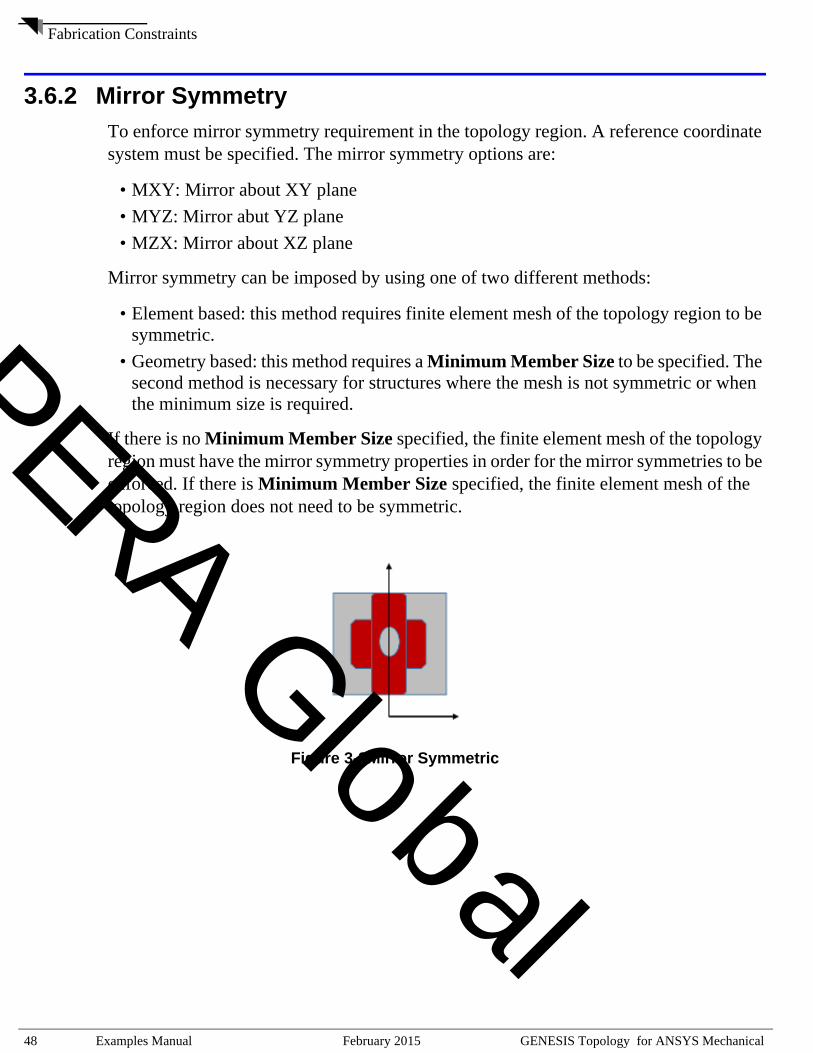
Fabrication Constraints
PE
3.6.2 Mirror SymmetryTo enforce mirror symmetry requirement in the topology region. A reference coordinate system must be specified. The mirror symmetry options are:
• MXY: Mirror about XY plane• MYZ: Mirror abut YZ plane• MZX: Mirror about XZ plane
Mirror symmetry can be imposed by using one of two different methods:
• Element based: this method requires finite element mesh of the topology region to be symmetric.
• Geometry based: this method requires a Minimum Member Size to be specified. The second method is necessary for structures where the mesh is not symmetric or when the minimum size is required.
If there is no Minimum Member Size specified, the finite element mesh of the topology region must have the mirror symmetry properties in order for the mirror symmetries to be enforced. If there is Minimum Member Size specified, the finite element mesh of the topology region does not need to be symmetric.
Figure 3-3Mirror Symmetric
安世
亚太
RA Global
48 Examples Manual February 2015 GENESIS Topology for ANSYS Mechanical
Fabrication Constraints
PE
3.6.3 Cyclic SymmetryTo enforce cyclic symmetry in the topology region. A reference coordinate system must be specified. The cyclic symmetry options are:
• CX: Cyclic about X axis• CY: Cyclic abut Y axis• CZ: Cyclic abut Z axis
Cyclic symmetry can be imposed by using one of two different methods:
• Element based: this method requires finite element mesh of the topology region to be cyclic symmetric.
• Geometry based: this method requires a Minimum Member Size to be specified. The second method is necessary for structures where the mesh is not cyclic symmetric or when the minimum size is required.
If no Minimum Member Size specified, the finite element mesh of the topology region must have the cyclic symmetry properties in order for the cyclic symmetries to be achieved. If Minimum Member Size is specified, the finite element mesh of the topology region does not need to be cyclic symmetric.
The user need to specify the number of cyclic symmetries. For example, there are 5 cyclic symmetric sections as shown in Figure 3-4.
Figure 3-4Topology Region with 5 Cyclic Symmetric Sections
安世
亚太
RA Global
GENESIS Topology for ANSYS Mechanical February 2015 Examples Manual 49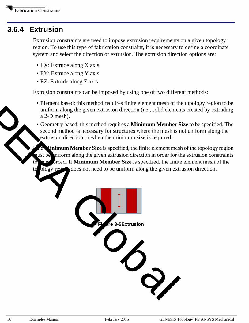
Fabrication Constraints
PE
3.6.4 ExtrusionExtrusion constraints are used to impose extrusion requirements on a given topology region. To use this type of fabrication constraint, it is necessary to define a coordinate system and select the direction of extrusion. The extrusion direction options are:
• EX: Extrude along X axis• EY: Extrude along Y axis• EZ: Extrude along Z axis
Extrusion constraints can be imposed by using one of two different methods:
• Element based: this method requires finite element mesh of the topology region to be uniform along the given extrusion direction (i.e., solid elements created by extruding a 2-D mesh).
• Geometry based: this method requires a Minimum Member Size to be specified. The second method is necessary for structures where the mesh is not uniform along the extrusion direction or when the minimum size is required.
If no Minimum Member Size is specified, the finite element mesh of the topology region must be uniform along the given extrusion direction in order for the extrusion constraints to be enforced. If Minimum Member Size is specified, the finite element mesh of the topology region does not need to be uniform along the given extrusion direction.
Figure 3-5Extrusion
安世
亚太
RA Global
50 Examples Manual February 2015 GENESIS Topology for ANSYS Mechanical
Fabrication Constraints
PE
3.6.5 FillingFilling constraints are used to impose fabrication requirements, such as castability, where it is important that a part does not “lock the mold”. This constraint is imposed by requiring that material can only be added into the region by “filling up” in a given direction. To use this type of fabrication constraints it is necessary to define a coordinate system and select the filling direction (mold pull-off direction). It is always required to specify a Minimum Member Size for this type of fabrication constraints. The filling options (Figure 3-6) are:
Filling from the bottom plane
• FBX: Filling X axis (- to +)• FBY: Filling Y axis (- to +)• FBZ: Filling Z axis (- to +)
Filling from the top plane
• FTX: Filling X axis (+ to -)• FTY: Filling Y axis (+ to -)• FTZ: Filling Z axis (+ to -)
Filling simultaneous from top and bottom plane
• FSX: Filling X axis (outside to in)• FSY: Filling Y axis (outside to in)• FSZ: Filling Z axis (outside to in)
Filling from the general plane
• FGX: Filling X axis (inside to out)• FGY: Filling Y axis (inside to out)• FGZ: Filling Z axis (inside to out)
Filling symmetrically from the given plane
• F0X: Filling X axis (plane to - and +)• F0Y: Filling Y axis (plane to - and +)• F0Z: Filling Z axis (plane to - and +)
安世
亚太
RA Global
GENESIS Topology for ANSYS Mechanical February 2015 Examples Manual 51
Fabrication Constraints
PE
Figure 3-6Filling Options
Red (Dark) is the material to keep, in blue (light) are the voids.
X
YZ
安世
亚太
RA Global
52 Examples Manual February 2015 GENESIS Topology for ANSYS Mechanical
Fabrication Constraints
PE
3.6.6 Sheet FormingSheet forming constraints are used to impose fabrication requirements, so that the final structure can be built using one or two stamped sheets. To use this type of fabrication constraints it is necessary to define a coordinate system and select the stamping direction. It is always required to specify a Minimum Member Size for this type of fabrication constraints. The stamping options are:
Stamping with one sheet from the bottom
• SBX: Sheet normal to X axis• SBY: Sheet normal to Y axis• SBZ: Sheet normal to Z axis
Stamping with one sheet from the top
• STX: Sheet normal to X axis• STY: Sheet normal to Y axis• STZ: Sheet normal to Z axis
Stamping with two sheets simultaneous from top and bottom
• S2X: Two sheets normal to X axis• S2Y: Two sheets normal to Y axis• S2Z: Two sheets normal to Z axis
Figure 3-7 shows stamping options in Z direction.
Figure 3-7Stamping Options in Z direction
Additional parameters include:
• Sheet thicknessThe user must specify a thickness for the stampable sheet. The value of the thickness can be specified in two ways: Real > 0 or -1.0≤Real<0. A positive value enters the exact value of the thickness. A negative value will cause the
X
YZ
S2Z SBZ STZ
安世
亚太
RA Global
GENESIS Topology for ANSYS Mechanical February 2015 Examples Manual 53
Fabrication Constraints
PE
program to calculate the thickness as a fraction of the local height, where the fraction is the given thickness value.
• Allow through holesThe user can have holes or no hole option. Default is YES.
• Void valueDensity of the void area. The default value is 0.001. In general, the user does not need to change this value.
• Start offsetStarting location of the sheet. The offset is given as a fraction value (0≤Real≤1.0), which is the fraction of the local height away from the top and/or bottom. Default=0.0.
安世
亚太
RA Global
54 Examples Manual February 2015 GENESIS Topology for ANSYS Mechanical
Fabrication Constraints
PE
3.6.7 UniformTo enforce uniform requirement in planes parallel to a given plane or in all directions.
Uniform in planes parallel to a given plane (Figure 3-8):
• UXY: Uniform in planes parallel to XY plane• UYZ: Uniform in planes parallel to YZ plane• UXZ: Uniform in planes parallel to XZ plane
Figure 3-8Uniform in planes parallel to a given plane
Uniform in all directions (UXYZ):
In this case, elements in the whole design region is controlled by one design variable. As a result, topology optimization will either keep or remove this region.
Figure 3-9Uniform in all directions
Uniform in planes constraints can be imposed by using one of two different methods:
• Element based: this method requires finite element mesh of the topology region to be uniform in planes parallel to the given plane (i.e., solid elements created by extruding a 2-D mesh).
• Geometry based: this method requires a Minimum Member Size to be specified. The second method is necessary for structures where the mesh is not uniform in planes parallel to the given plane or when the minimum size is required.
安世
亚太
RA Global
GENESIS Topology for ANSYS Mechanical February 2015 Examples Manual 55
Fabrication Constraints
PE
If no Minimum Member Size is specified, the finite element mesh of the topology region must be uniform in planes parallel to the given plane in order for the UXY, UYZ or UXZ constraints to be enforced. If Minimum Member Size is specified, the finite element mesh of the topology region does not need to be uniform in planes parallel to the given plane. 安
世亚
太 RA Global
56 Examples Manual February 2015 GENESIS Topology for ANSYS Mechanical

Fabrication Constraints
PE
3.6.8 Radial FillingTo enforce filling constraints radially. This constraint is imposed by requiring that material can only be added into the region by “filling up” in a given direction radially. To use this type of fabrication constraints it is necessary to define a coordinate system and select the filling direction (mold pull-off direction). It is also required to specify a Minimum Member Size. The filling options (Figure 3-10) are:
Radially filling from the inner surface
• RBX: radially filling from the inner surface about X axis• RBY: radially filling from the inner surface about Y axis• RBZ: radially filling from the inner surface about Z axis
Radially filling from the outer surface
• RTX: radially filling from the outer surface about X axis• RTY: radially filling from the outer surface about Y axis• RTZ: radially filling from the outer surface about Z axis
Radially filling from the general surface
• RGX: radially filling from the general surface about X axis• RGY: radially filling from the general surface about Y axis• RGZ: radially filling from the general surface about Z axis
Figure 3-10Radially filling about (perpendicular to the) Z axis
Red (Dark) is the material to keep, in gray (light) are the voids.
RBZ RTZ RGZ
Z Z Z
安世
亚太
RA Global
GENESIS Topology for ANSYS Mechanical February 2015 Examples Manual 57
Fabrication Constraints
PE
An additional parameter to for this type of constraints is the Number of Radial Candidates. This parameter controls in how many sectors the topology region is divided. The larger this parameter, the larger the number of design variables are used and the more design freedom is given to the problem. Typical values that can be used for this parameter are 30, 60, 90 or 360.
When a cyclic symmetry constraints is used together with a radial filling constraint then the number of radial candidates need to be a multiple of the number of cyclic symmetries used. For example, if the number of cyclic of symmetries is 5, then the number of radial candidates could be 30 (5*6), 35(5*7), 200(5*20), and etc.
安世
亚太
RA Global
58 Examples Manual February 2015 GENESIS Topology for ANSYS Mechanical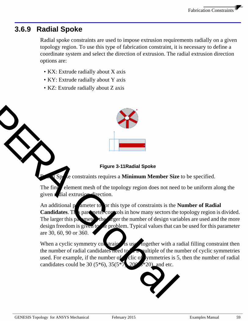
Fabrication Constraints
PE
3.6.9 Radial SpokeRadial spoke constraints are used to impose extrusion requirements radially on a given topology region. To use this type of fabrication constraint, it is necessary to define a coordinate system and select the direction of extrusion. The radial extrusion direction options are:
• KX: Extrude radially about X axis• KY: Extrude radially about Y axis• KZ: Extrude radially about Z axis
Figure 3-11Radial Spoke
Radial Spoke constraints requires a Minimum Member Size to be specified.
The finite element mesh of the topology region does not need to be uniform along the given radial extrusion direction.
An additional parameter to for this type of constraints is the Number of Radial Candidates. This parameter controls in how many sectors the topology region is divided. The larger this parameter, the larger the number of design variables are used and the more design freedom is given to the problem. Typical values that can be used for this parameter are 30, 60, 90 or 360.
When a cyclic symmetry constraints is used together with a radial filling constraint then the number of radial candidates need to be a multiple of the number of cyclic symmetries used. For example, if the number of cyclic of symmetries is 5, then the number of radial candidates could be 30 (5*6), 35(5*7), 200(5*20), and etc.
安世
亚太
RA Global
GENESIS Topology for ANSYS Mechanical February 2015 Examples Manual 59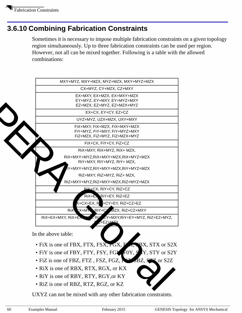
Fabrication Constraints
PE
3.6.10 Combining Fabrication ConstraintsSometimes it is necessary to impose multiple fabrication constraints on a given topology region simultaneously. Up to three fabrication constraints can be used per region. However, not all can be mixed together. Following is a table with the allowed combinations:
In the above table:
• FiX is one of FBX, FTX, FSX, FGX, F0X, SBX, STX or S2X• FiY is one of FBY, FTY, FSY, FGY, F0Y, SBY, STY or S2Y• FiZ is one of FBZ, FTZ , FSZ, FGZ, F0Z, SBZ, STZ or S2Z • RiX is one of RBX, RTX, RGX, or KX• RiY is one of RBY, RTY, RGY,or KY• RiZ is one of RBZ, RTZ, RGZ, or KZ
UXYZ can not be mixed with any other fabrication constraints.
MXY+MYZ, MXY+MZX, MYZ+MZX, MXY+MYZ+MZX
CX+MYZ, CY+MZX, CZ+MXY
EX+MXY, EX+MZX, EX+MXY+MZXEY+MYZ, EY+MXY, EY+MYZ+MXYEZ+MZX, EZ+MYZ, EZ+MZX+MYZ
EX+CX, EY+CY, EZ+CZ
UYZ+MYZ, UZX+MZX, UXY+MXY
FiX+MXY, FiX+MZX, FiX+MXY+MZXFiY+MYZ, FiY+MXY, FiY+MYZ+MXYFiZ+MZX, FiZ+MYZ, FiZ+MZX+MYZ
FiX+CX, FiY+CY, FiZ+CZ
RiX+MXY, RiX+MYZ, RiX+ MZX,
RiX+MXY+MYZ,RiX+MXY+MZX,RiX+MYZ+MZXRiY+MXY, RiY+MYZ, RiY+ MZX,
RiY+MXY+MYZ,RiY+MXY+MZX,RiY+MYZ+MZX
RiZ+MXY, RiZ+MYZ, RiZ+ MZX,
RiZ+MXY+MYZ,RiZ+MXY+MZX,RiZ+MYZ+MZX
RiX+CX, RiY+CY, RiZ+CZ
RiX+EX, RiY+EY, RiZ+EZ
RiX+CX+EX, RiY+CY+EY, RiZ+CZ+EZ
RiX+CX+MYZ, RiY+CY+MZX, RiZ+CZ+MXY
RiX+EX+MXY, RiX+EX+MZX, RiY+EY+MXY,RiY+EY+MYZ, RiZ+EZ+MYZ, RiZ+EZ+MZX,
安世
亚太
RA Global
60 Examples Manual February 2015 GENESIS Topology for ANSYS Mechanical
Fabrication Constraints
PE
The user does not need to memorize all the possible combinations. For the three lists where the fabrication constraints are selected from in the GUI, the program will automatically filter out the non-compatible fabrication constraints based on what has already been selected.
安世
亚太
RA Global
GENESIS Topology for ANSYS Mechanical February 2015 Examples Manual 61
Fabrication Constraints
PE
3.6.11 List of All Fabrication ConstraintsTYPE Description of Fabrication Constraints
MXY Mirror symmetry with respect to the XY plane
MYZ Mirror symmetry with respect to the YZ pane
MZX Mirror symmetry with respect to the ZX plane
CX Cyclic symmetry about the X axis
CY Cyclic symmetry about the Y axis
CZ Cyclic symmetry about the Z axis
EX Extrusion along the X axis
EY Extrusion along the Y axis
EZ Extrusion along the Z axis
UXY Uniform in planes parallel to the XY plane
UYZ Uniform in planes parallel to the YZ pane
UZX Uniform in planes parallel to the ZX plane
UXYZ Uniform in all directions
FBX Filling in the +X direction
FBY Filling in the +Y direction
FBZ Filling in the +Z direction
FTX Filling in the -X direction
FTY Filling in the -Y direction
FTZ Filling in the -Z direction
FSX Filling simultaneously from +X and -X directions(filling from the outside in)
FSY Filling simultaneously from +Y and -Y directions(filling from the outside in)
FSZ Filling simultaneously from +Z and -Z directions(filling from the outside in)
FGX Filling on +X and -X directions from general surface(filling from the inside out)
FGY Filling on +Y and -Y directions from general surface(filling from the inside out)
FGZ Filling on +Z and -Z directions from general surface(filling from the inside out)
安世
亚太
RA Global
62 Examples Manual February 2015 GENESIS Topology for ANSYS Mechanical
Fabrication Constraints
PE
F0X Filling symmetrically from X=0.0 toward the top and bottom
(filling from the inside out)
F0Y Filling symmetrically from Y=0.0 toward the top and bottom
(filling from the inside out)
F0Z Filling symmetrically from Z=0.0 toward the top and bottom
(filling from the inside out)
RBX Radial Filling From the Inner Surface about the X axis
RBY Radial Filling From the Inner Surface about the Y axis
RBZ Radial Filling From the Inner Surface about the Z axis
RTX Radial Filling From the Outer Surface about the X axis
RTY Radial Filling From the Outer Surface about the Y axis
RTZ Radial Filling From the Outer Surface about the Z axis
RGX Radial Filling From the General Surface about the X axis
(from the interior to the inner and outer surfaces)
RGY Radial Filling From the General Surface about the Y axis
(from the interior to the inner and outer surfaces)
RGZ Radial Filling From the General Surface about the Z axis
(from the interior to the inner and outer surfaces)
KX Radial Spokes about the X axis
KY Radial Spokes about the Y axis
KZ Radial Spokes about the Z axis
SBX Sheet forming normal to +X (1 Layer)
(initial configuration starts at the bottom)
SBY Sheet forming normal to +Y (1 Layer)
(initial configuration starts at the bottom)
SBZ Sheet forming normal to +Z (1 Layer)
(initial configuration starts at the bottom)
STX Sheet forming normal to +X (1 Layer)
(initial configuration starts at the top)
STY Sheet forming normal to +Y (1 Layer)
(initial configuration starts at the top)
STZ Sheet forming normal to +Z (1 Layer)
(initial configuration starts at the top)
安世
亚太
RA Global
GENESIS Topology for ANSYS Mechanical February 2015 Examples Manual 63
Fabrication Constraints
PE
S2X Sheet forming normal to +X (2 Layer)
(initial configuration of first layer starts at the top;
initial configuration of second layer starts at the bottom)
S2Y Sheet forming normal to +Y (2 Layer)
(initial configuration of first layer starts at the top;
initial configuration of second layer starts at the bottom)
S2Z Sheet forming normal to +Z (2 Layer)
(initial configuration of first layer starts at the top;
initial configuration of second layer starts at the bottom)
安世
亚太
RA Global
64 Examples Manual February 2015 GENESIS Topology for ANSYS Mechanical
Fabrication Constraints
PE
3.6.12 Minimum Size Control
Minimum Member SizeMinimum Member Size is the desired minimum dimension of any resultant topology component. The recommended value should be at least twice of the element size. Using a larger value for minimum member size results in fewer design variables.
Minimum Member Size is used for two purposes. The first purpose is straight forward: to define the minimum member size of the final structure. The second purpose is to activate geometry based topology design method, which is required for certain manufacture constraints such as filling and stamping, or helps enforce manufacturing constraints on topology regions where meshes are not compatible with the given constraints. These cases are described as follows:
• Symmetry on a mesh that are not symmetric• Cyclic symmetry on a mesh that are not cyclic symmetric• Extrusion on a mesh that is not uniform along the given extrusion direction (i.e. solid
elements created by extruding a 2-D mesh) • Filling constraints always require a minimum member size• Sheet forming constraints always require a minimum member size• Uniform in parallel planes on a mesh that is not uniform in planes parallel to the given
plane (i.e., solid elements created by extruding a 2-D mesh).• Radial filling constraints always require a minimum member size• Radial spoke constraints on a mesh that is not uniform along the radial extrusion
direction
Minimum member size is optional for problems without manufacturing constraints or problems that do have manufacturing constrain but have uniform meshes that are compatible with the manufacturing constraint.
When minimum member size is specified, geometry based topology design method is used. Otherwise, element based method is used.
Spread FractionSpread Fraction is a parameter that allows smoother result in topology. The value ranges from 0.0 to 1.0. Typical values are 0.0 or 0.5. A value of 0.0 will cause no smoothing. A value of 0.5 produces smoother results.
For example in Figure 3-12, topology result with no spread fraction (left) is more zig-zag on the edge than the one with spread faction (right).
安世
亚太
RA Global
GENESIS Topology for ANSYS Mechanical February 2015 Examples Manual 65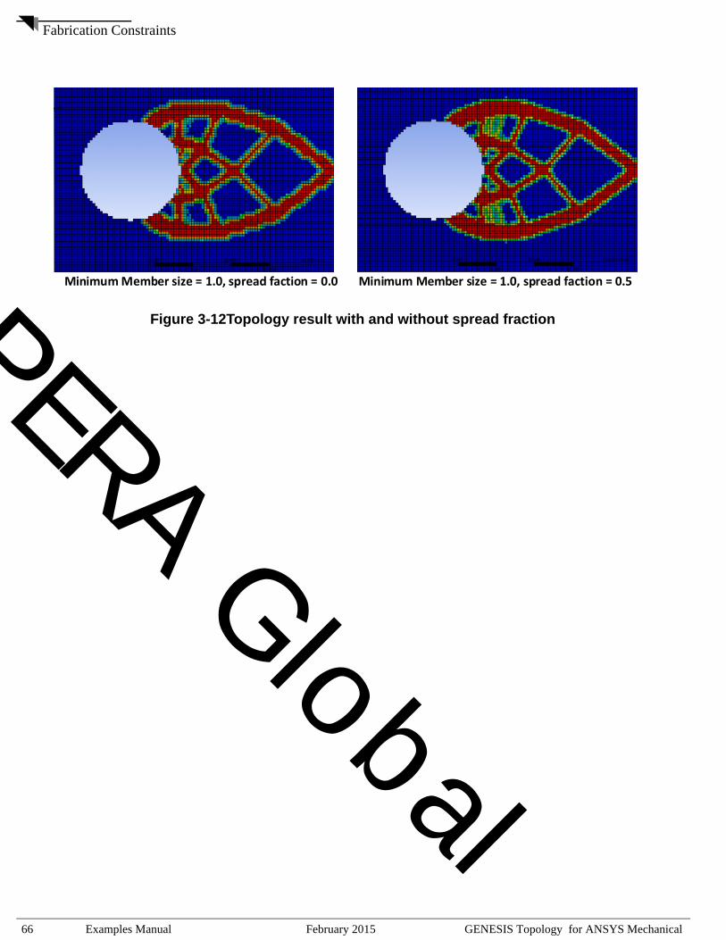
Fabrication Constraints
PE
Figure 3-12Topology result with and without spread fractionMinimum Member size = 1.0, spread faction = 0.0 Minimum Member size = 1.0, spread faction = 0.5
安世
亚太
RA Global
66 Examples Manual February 2015 GENESIS Topology for ANSYS Mechanical
Fabrication Constraints
PE
3.6.13 Maximum Size Control
Maximum Member SizeMaximum Member Size is the desired maximum dimension of any resultant topology component. This help reduce local mass concentrations. Typically, Maximum member size should be 3 times the size of minimum member size.
Please note that the use of maximum member size should be restricted when it is necessary. The reason is that maximum member size control reduces the design freedom and increases the computation time. It is interesting to note that minimum member size does not increase computational cost.
The use of maximum member size requires the use of minimum gap which is explained next.
Minimum GapMinimum Gap helps to separate topology generated members so that they are not too close to each other. Minimum gap is required when Maximum Member Size is used. The default value for minimum gap is the same value as Maximum Member Size. When Maximum Member Size is not used, then Minimum Gap is not used either.
Figure 3-13Topology result with and without maximum size control
With Maximum Member Size ControlW/O Maximum Member Size Control
安世
亚太
RA Global
GENESIS Topology for ANSYS Mechanical February 2015 Examples Manual 67
Analysis Settings
PE
3.7 Analysis SettingsIn Analysis Settings, the user can set parameters for:
• Design Control• Design Move Limits• Design Convergence• Design Methods• Analysis Control• Design Output Control• Analysis Output Control• Post-Processing Control• Coarsened Surface• Modal/Buckling Analysis• Random Response• Random Output• Non-linear Contact
安世
亚太
RA Global
68 Examples Manual February 2015 GENESIS Topology for ANSYS Mechanical
Analysis Settings
PE
3.7.1 Design Control
Max. Design Cycles (DESMAX)To specify the maximum allowable number of design cycles for optimization problem. Default value is 15.
If the initial design is far from the optimum design this value should be raised. It should also be raised if the responses are very nonlinear functions of the design variables. If the analysis is very expensive, it is advisable to set DESMAX to a smaller number.
If the maximum number of design cycles is reached, the design process can always be continued using the GENESIS restart capability. The restart capability is explained in Restart Optimization.
安世
亚太
RA Global
GENESIS Topology for ANSYS Mechanical February 2015 Examples Manual 69
Analysis Settings
PE
3.7.2 Design Move LimitsGENESIS topology optimization uses an approximate problem to solve the optimization problem more efficiently. In general, the approximations are accurate close to the design variable value at which they were constructed. This makes it necessary to limit the range of design variable values for which the approximations are used. These limits will be used as temporary bounds in a particular design cycle. At the end of the optimization the move limits should not have affected the results. The data to specify these move limits are Fractional Move Limit (DELT) and Minimum Move Limit (DTMIN). The temporary bounds created using move limits at design cycle i for design variable X are:
Where TMIN is minimum value of topology design variable.
Fractional Move Limit (DELT)Fractional change allowed for each designable topology variable during the approximate optimization. Default value is 1.0E-6.
Min. Move Limit (DTMIN)Minimum move limit fraction imposed for topology design variables at a given design cycle. Default values is 0.2.
When to Change Move LimitsIn general the move limits work well for most of the problem and the user does not need to change the move limits values.
A special case where changing the move limits value is recommended is when the initial mass fraction is less than 10%. In this case, the recommended move limits value are DELT=0.4, DTMIN=(Initial Mass Fraction)/3.0. When smaller move limits are used, the problem will take more design cycles to converge. So in this case, it is also recommended to increase the maximum number of design cycles.
LBi MAX TMIN Xi MAX DELT*Xi DTMIN,( )–,[ ]=
UBi MIN 1.0 Xi MAX DELT*Xi DTMIN,( )+,[ ]=
安世
亚太
RA Global
70 Examples Manual February 2015 GENESIS Topology for ANSYS Mechanical
Analysis Settings
PE
3.7.3 Design Convergence
Hard ConvergenceThere are two conditions that must be met for hard convergence. The first is that all the design constraints must not be violated by more than a small value Hard Max. Violation (GMAX). The other condition is that either the relative change in the objective function for two consecutive design cycles be less than Hard Relative (CONV1) or the absolute change in the objective function for two consecutive design cycles be less than Hard Absolute (CONV2). If the user wishes to get very close to the optimum design, the values of CONV1 and CONV2 can be made smaller. Larger values of CONV1 and CONV2 will lead to faster convergence but the final design may not be optimum. The maximum allowable constraint violation can also be reduced or increased. It is not recommended that GMAX be made smaller than 0.003.
Hard Relative (CONV1)Relative change criterion to detect hard convergence of the overall optimization process. Terminate if the relative change in the objective function is less than CONV1 for two consecutive design cycles and all constraints are satisfied. Default value is 0.001.
Hard Absolute (CONV2)Absolute change criterion to detect hard convergence of the overall optimization process. Terminate if the absolute change in the objective function is less than CONV2 for two consecutive design cycles and all constraints are satisfied. Default value is 0.001.CONV2 = Max(CONV2*Objinitial, 1.0E-19)This means that it is the maximum of 0.1% of the initial objective function value or 1.0E-19.
Hard Max. Violation (GMAX)Maximum constraint violation allowed at optimum. Constraints are normalized so a value of 0.01 represents a one percent constraint violation. Default value is 0.005.
安世
亚太
RA Global
GENESIS Topology for ANSYS Mechanical February 2015 Examples Manual 71
Analysis Settings
PE
Soft ConvergenceThere are two conditions that must be met for soft convergence. The first is that all the design constraints must not be violated by more than a small value Soft Constraint (CONVCN). The other condition is that the relative change in the design variables for two consecutive design cycles be less than Soft Relative (CONVDV).
Soft Constraint (CONVCN)Allowable change in the maximum constraint value for soft convergence. Default value is 0.001. If the change in the maximum constraint value is less than CONVCN, and CONVDV are satisfied, then terminate the design process with soft convergence.
Soft Variable (CONVDV)Relative change criterion to detect soft convergence of the overall optimization process. Default value is 0.001. Terminate with soft convergence if the maximum relative change in the design variables is less than CONVDV during the approximate optimization and CONVCN are satisfied.
Hard Convergence vs. Soft ConvergenceFrom an engineering viewpoint, hard convergence is probably better because it indicates that the design is more robust: small changes in the design variables will not have a big effect on the objective and constraint functions.
安世
亚太
RA Global
72 Examples Manual February 2015 GENESIS Topology for ANSYS Mechanical
Analysis Settings
PE
3.7.4 Design Methods
Topology Index (TINDEXM)The compliance index objective function is a weighted sum of response terms. How each term enters into the objective function depends of the parameter Topology Index (TINDEXM).
If Topology Index is Normalized Reciprocal (TINDEXM=0) or Normalized Direct (TINDEXM=1), then responses are normalized by their values in the first design cycle. If Topology Index is Reciprocal (TINDEXM=2) or Direct (TINDEXM=3), then responses are not normalized.
• TINDEXM = 0 or 1
(Eq. 3-4)
• TINDEXM = 2 or 3
(Eq. 3-5)
The compliance index objective function is calculated using the following equation:
(Eq. 3-6)
If Topology Index is Normalized Reciprocal (TINDEXM=0) or Reciprocal (TINDEXM=2), then the compliance index objective function terms are calculated using reciprocals for negative weighting factors (maximizing a response value). If Topology Index is Normalized Direct (TINDEXM=1) or Direct (TINDEXM=3), then the compliance index objective function is a straight summation.
• TINDEXM = 0 or 2
(Eq. 3-7)
• TINDEXM = 1 or 3
(Eq. 3-8)
RiResponseiResponse0i--------------------------------=
Ri Responsei=
T fii 1=∑=
fi
Wi Ri⋅ if Wi 0>
W– iRi
--------- if Wi 0<⎩⎪⎨⎪⎧
=
fi WiRi=
安世
亚太
RA Global
GENESIS Topology for ANSYS Mechanical February 2015 Examples Manual 73
Analysis Settings
PE
Anticheckerboard FilterAnticheckerboard Filter is used to prevent having a result that looks like a checker board.
Figure 3-14Topology result with and without anticheckerboard control
安世
亚太
RA Global
74 Examples Manual February 2015 GENESIS Topology for ANSYS Mechanical
Analysis Settings
PE
As shown in Figure 3-14, the result in the top picture has anticheckerboard control.
Anticheckerboard Filter (FILTER)• Global
GENESIS uses a global anticheckerboard filter region.• Regional
GENESIS uses property-by-property (body-by-body) anticheckerboard filter regions.
• Regional with Norm CheckGENESIS will use property-by-property (body-by-body) anticheckerboard filter regions and it will take in consideration the angle of the norms of shell elements to determine the neighbor influences. The more closely aligned neighbor element norms are, the stronger those elements will interact in the filter. Orthogonal elements will not interact. For non-shell elements, the option Regional with Norm Check has same effect as Regional. Parameter Cutoff Angle (FILTNRM) can be used withRegional with Norm Check to further limit the number of elements that interact.
• OffThe anticheckerboard filter is turned off.
Cutoff Angle (FILTNRM)Cutoff angle to exclude neighbor elements from participating in an anti-checkerboard filter region. In nonplanar structures, smaller values of FILTNRM reduces the number of elements in a checkerboard region. Conversely, larger values of FILTNRM increases the number of elements in checkerboard region.
A value of 0.0 will force GENESIS to create anticheckerboard filter regions containing only neighbor elements in the same plane. A value of 90.0 will let GENESIS include all neighbor elements (however elements close to 90 degree will have little to no influence).
This parameter is only used with Regional with Norm Check option and it is ignored with other filter options.
This parameter is only used with shell elements and it is ignored with other types.
Linearization (LINAPR)Approximation Optimization Method Control.
安世
亚太
RA Global
GENESIS Topology for ANSYS Mechanical February 2015 Examples Manual 75
Analysis Settings
PE
Regular (LINAPR = 0) will cause the program to use the “fast” linear approximations method when all approximations are linear. If any approximations are nonlinear, then the program will use its standard hybrid approximations. Aggressive (LINAPR = 1) will force the program to use the “fast” linear approximations method for all responses. This will result in faster times in each design cycle, but it might lower the quality of approximations which in some cases might cause the program to need more design cycles to converge.
By default, Regular option is used.安世
亚太
RA Global
76 Examples Manual February 2015 GENESIS Topology for ANSYS Mechanical
Analysis Settings
PE
3.7.5 Analysis Control
ProcessorsNumber of processors used by GENESIS solver. Default value is 2.
MemoryMemory (MB) used by GENESIS solver. By default, half of the memory will be used.
Diag. LevelThe diagnosis output level, which is in format:
d1, d2, d3, ...
where di is the command switch. For example, 85 is to print problem summary, and 87 is to print most detailed summary. For more details please refer to GENESIS Analysis Manual.
GENESIS Solver
OptimizeGENESIS solver will be called to solve the optimization problem.
If there is result object in the tree, the corresponding result files will be read back to ANSYS mechanical for post-processing. The density file name is in format of genesisDENXX.pch, and the analysis result file name is in format of genesisXX.pch, where ‘XX’ means design cycle.
Single AnalysisGENESIS solver will be called to solve the analysis problem only.
Note that the Init. Mass Fraction is used in analysis too.
Dry run to import results
安世
亚太
RA Global
GENESIS Topology for ANSYS Mechanical February 2015 Examples Manual 77
Analysis Settings
PE
Only the result files are read back to ANSYS mechanical. This option shall be used in case the optimization problem is solved externally using GENESIS. The user need to specify the location of GENESIS output file (e.g., genesis.out), the density file (e.g., genesisDENXX.pch), and the analysis result file (e.g., genesisXX.pch), where ‘XX’ means design cycle.
Restart OptimizationThe restart capability allows the user to restart from any previous design cycle. By default the optimization restarts from the last design cycle. The user can also specify a maximum number of design cycles allowed for restarted optimization. Note that this is the additional number of design cycles the optimization will run further.
For the restarted optimization, the last analysis in previous optimization is repeated, but the user can change the input data. The only restriction on the input data for the restart is that the number and order of the design variables remains constant. The restart uses the genesis.HIS file that is created after every run.
If GENESIS reaches the maximum number of design cycles, the user may want to restart optimization from a previous design cycle. Before restarting, the user should examine the objective function history. If the value of the objective function is oscillating or if the maximum constraint violation oscillates, the user may try
• reduce the move limits or • increase the constraint screening parameters
then restart from the best design in the design history table.
If restart is used, two sets of information will be lost
• Mode tracking• Automatic move limit adjustments
Write New GENESIS Input FileBy default a new GENESIS input file is written every time the solution is solved. Optionally the user can choose not writing out a new file incase the user manually modified some data in the input file and would like to solve using the modified file directly.
安世
亚太
RA Global
78 Examples Manual February 2015 GENESIS Topology for ANSYS Mechanical
Analysis Settings
PE
GENESIS Solver ExecutableThe location of the GENESIS executable. By default, the latest version of GENESIS that is installed in current machine will be shown. However, the user can edit the GENESIS solver location if it is necessary.
Design Studio ExecutableThe location of the Design Studio executable. By default, the latest version of Design Studio that is installed in current machine will be shown. However, the user can edit the Design Studio location if it is necessary.
安世
亚太
RA Global
GENESIS Topology for ANSYS Mechanical February 2015 Examples Manual 79
Analysis Settings
PE
3.7.6 Design Output Control
Topology DensityThe topology design variable values (volume fraction) for each element may optionally be printed in a post processing file named pnameDENSxx.ext, where pname is set to the base of the input filename, xx is the design cycle number, and ext is set according to the file format. The extension of the filename is based on the format: op2 for OUTPUT2 format (binary), pch for PUNCH format (ASCII). Currently, GTAM only exports file in PUNCH format with extension pch.
Topology Density result is always requested in GTAM.
Output for Design CyclesThe user can also control if requesting results for all design cycles or only part of it. By default, topology density results for all design cycles are requested.
• AllTopology density results for all design cycles are requested
• First and LastTopology density results for first and last design cycles are requested
• LastOnly the last design cycle result is requested
安世
亚太
RA Global
80 Examples Manual February 2015 GENESIS Topology for ANSYS Mechanical
Analysis Settings
PE
3.7.7 Analysis Output ControlTo turn on/off output for Deformation, Stress, Strain, Velocity and Acceleration. These analysis results may optionally be printed in a post processing file named pnamexx.ext, where pname is set to the base of the input filename, xx is the design cycle number, and ext is set according to the file format. The extension of the filename is based on the format: op2 for OUTPUT2 format (binary), pch for PUNCH format (ASCII). Currently, GTAM only exports file in PUNCH format with extension pch.
The user can also control if writing results for all design cycles or only part of it.
DeformationTo turn on/off output for Deformation. The deformation values for each grid may optionally be printed in a post processing file named pnamexx.ext.
Element StressTo turn on/off output for Element Stress. The element stress values for each element may optionally be printed in a post processing file named pnamexx.ext.
Grid StressTo turn on/off output for Grid Stress. The grid stress values for each grid may optionally be printed in a post processing file named pnamexx.ext.
StrainTo turn on/off output for Strain. The element strain values for each element may optionally be printed in a post processing file named pnamexx.ext.
Strain EnergyTo turn on/off output for Strain Energy. The element strain energy values for each element may optionally be printed in a post processing file named pnamexx.ext.
VelocityTo turn on/off output for Velocity. The dynamic velocity values for each grid may optionally be printed in a post processing file named pnamexx.ext.
安世
亚太
RA Global
GENESIS Topology for ANSYS Mechanical February 2015 Examples Manual 81
Analysis Settings
PE
AccelerationTo turn on/off output for Acceleration. The dynamic acceleration values for each grid may optionally be printed in a post processing file named pnamexx.ext.
Output for Design CyclesThe user can also control if requesting results for all design cycles or only part of it. By default, results for first and last design cycles are request.
• AllResults for all design cycles are requested
• First and LastResults for first and last design cycles are requested
• LastOnly the last design cycle result is requested
安世
亚太
RA Global
82 Examples Manual February 2015 GENESIS Topology for ANSYS Mechanical
Analysis Settings
PE
3.7.8 Post-Processing Control
Import for Design CyclesTo control if importing results for all design cycles or only part of it for post-processing. By default, only the last design cycle results are imported for post-processing.
• AllResults for all design cycles are imported for post-processing. Please note that if the user does not request all design cycles results in output, the program will only import what is available in the output file.
• First and LastResults for first and last design cycles are imported for post-processing. Please note that if the user does not request first and last design cycles results in output, the program will only import what is available in the output file.
• LastOnly the last design cycle result is imported for post-processing.
安世
亚太
RA Global
GENESIS Topology for ANSYS Mechanical February 2015 Examples Manual 83
Analysis Settings
PE
3.7.9 Coarsened SurfaceOnce the optimization finished, the user can export topology density isosurface in format of STL or IGES. Please not that only the external surface is exported.
Cut Off ValueTo specify a density level which will be used to construct the topology density isosurface.
A surface is generated such that it passes throughout the model wherever the element density has the specified cut off value, and encloses all regions where the density is greater than the given value.
The user need to set the cut off value at the Capped Isosurface toolbar.
Level of DetailsTo control the coarsening on the exported density isosurface. A smoothing algorithm is applied to this surface to produce the final output. 0 means maximum coarsening and 20 means no coarsening.
File TypeExport the isosurface in STL or IGES format.
Note that for IGES only the facet data is provided.
安世
亚太
RA Global
84 Examples Manual February 2015 GENESIS Topology for ANSYS Mechanical
Analysis Settings
PE
3.7.10 Modal/Buckling Analysis
Eigenvalue MethodTwo methods are available as the eigenvalue solver:
• Lanczos• SMS
SMS method requires the user to specify a frequency search range. If there is no range specified in the modal analysis settings, the program will default to Lanczos.
Mode TrackingMode tracking of Natural Frequencies or Buckling Load Factors control. The options are:
• Yes: the modes with constrained frequencies or buckling load factors are tracked• All: all modes are tracked• No: do not use mode tracking
NO is the default and does not enable mode tracking.
Natural Frequency LoadcasesAs the design changes throughout the design process, the order of the mode shapes can change. For example, initially the first bending mode of a structure could be at 7 Hz and the first torsional mode could be at 10 Hz. After the design is modified the first bending mode could be 11 Hz and the first torsional mode could be at 9 Hz. If a constraint was originally placed on the first bending mode, it would now be on the first torsional mode. Using mode tracking GENESIS can reorder the modes so that the constraint will remain on the first bending mode.
If a constrained mode that is being tracked is not found during a design cycle analysis, then a fatal error will be issued and GENESIS will stop.
If a constrained mode that is being tracked may have switched with another mode, then a warning message will be issued after design convergence. In this case the user should check the results of the last analysis to make sure that the correct mode shape was constrained.
If modes switch position during the design process the frequencies and mode shapes in the output and postprocessing files will not be in order of increasing frequency.
安世
亚太
RA Global
GENESIS Topology for ANSYS Mechanical February 2015 Examples Manual 85
Analysis Settings
PE
Mode tracking information will be printed in the analysis results section of the output file. It is important to examine this data if restarts optimization is going to be used. This is because the mode numbers which are referenced in the definition of objective or constraint will have to be changed if the mode switched order. The mode number in the design cycle to be restarted from will be the position of the mode when all of the modes are ordered from lowest to highest frequency.
It is typically needed to use mode tracking, whenever frequencies or eigenvector components are used as objective or constraints.
Buckling LoadcasesMode tracking can also be used to track modes associated to buckling analysis. The use of mode tracking in this case is very similar that with a natural frequency analysis and do not need further explanation.
In buckling optimization, however, it is not typically needed to use mode tracking as in most cases the key is to either raise the lowest buckling load factor or constraint it, and individual modes are not as important.
安世
亚太
RA Global
86 Examples Manual February 2015 GENESIS Topology for ANSYS Mechanical
Analysis Settings
PE
3.7.11 Random Response
Modal Max. Modes to Find• Program controlled
Default is 200• Use Definition in Modal
Will use Max. number of modes to find defined in Modal analysis
Modal Frequency Range• Program controlled
Will use double of the loading frequency range• Use Definition in Modal
Will use frequency range defined in Modal analysis
安世
亚太
RA Global
GENESIS Topology for ANSYS Mechanical February 2015 Examples Manual 87
Analysis Settings
PE
3.7.12 Random OutputTo turn on/off random output for Deformation, Stress, Strain, Velocity and Acceleration.
安世
亚太
RA Global
88 Examples Manual February 2015 GENESIS Topology for ANSYS Mechanical
Analysis Settings
PE
3.7.13 Non-linear Contact
Maximum Nonlinear IterationsMaximum number of solver iterations allowed for non-linear contact analysis.
Default is 25.
Penetration Tolerance FactorPenetration tolerance factor controls how much penetration is allowed. The actual allowable penetration at contact point is determined by this scale factor and average element size at the local contact region.
Default is 0.0001.
安世
亚太
RA Global
GENESIS Topology for ANSYS Mechanical February 2015 Examples Manual 89
Files Generated during Optimization Process
PE
3.8 Files Generated during Optimization Process
Summary of GENESIS Analysis and Design Files
xx = Design Cycle number
ext = op2, pch
Please note that by default the name of input file created in GTAM is genesis.dat.
INFORMATION CONTROL FILE NAME
Input Data created by user pname.dat
Output Data created always pname.out
Run Log created always pname.log
Analysis Post-Processing File request by user pnamexx.ext
Design History File created automatically pname.HIS
Restart Information File created automatically pname.RST
Design History Graph File created automatically pname.html
Topology Density File request by user pnameDENSxx.ext
安世
亚太
RA Global
90 Examples Manual February 2015 GENESIS Topology for ANSYS Mechanical
Files Generated during Optimization Process
PE
3.8.1 Program Output (pname.out)The results go to a file with the same base name as the input file and with the extension “.out”. If GENESIS stops because of an error, a detailed error message will be printed in the output file. The output file contains up to four sections.
In addition to the output file, Genesis will also create a log file (pname.log) that contains statistics about the system environment as well as any output that was printed to the terminal console. The log file also contains the exact start and stop times for the Genesis process, from which the total elapsed execution time can be calculated.
Model SummaryThis section contains tables of the analysis and design problem sizes and load case summary. The analysis table contains the number of grids, elements, degrees of freedom, etc. The load case table contains a summary with type and number of load cases.
Design ResultsThis section contains the design variable values, analysis model property values, and retained constraint response values for each design cycle.
Convergence InformationThis section contains the convergence information.
Design Cycle HistoryThis section contains an objective function history table which also includes the maximum constraint violation at each design cycle. Also included is the design variable value history. This is the last section of each run.
安世
亚太
RA Global
GENESIS Topology for ANSYS Mechanical February 2015 Examples Manual 91
Files Generated during Optimization Process
PE
3.8.2 Analysis Post-Processing File(pname.pch or pname.op2)Data for plotting displacements, velocities, accelerations, stresses, strains, mode shapes and etc can be generated by GENESIS. A separate file is written for each design cycle in which the analysis results have been requested. Only results that have been requested are written to the files.
The format of the post-processing files can be OUTPUT2 format or PUNCH format. Currently GTAM only supports PUNCH format.
The files have the name pnamexx.ext, where pname is set to the base of the input filename, xx is the design cycle number, and ext is op2 for OUTPUT2 format, pch for PUNCH format.
安世
亚太
RA Global
92 Examples Manual February 2015 GENESIS Topology for ANSYS Mechanical
Files Generated during Optimization Process
PE
3.8.3 Design Cycle History File (pname.HIS)This file has the name pname.HIS and contains the design cycle history. This is comprised of the objective function, maximum constraint violation, and design variable values for each design cycle. This is a formatted readable file and can be used to generate objective function and design variable history plots. This file is also used to restart the optimization. See Restart Optimization for more information. The last line of this file contains a completion code and the number of warnings and errors. The value of this code is 2 if there were errors, 1 if there were only warnings, and 0 otherwise.
安世
亚太
RA Global
GENESIS Topology for ANSYS Mechanical February 2015 Examples Manual 93
Files Generated during Optimization Process
PE
3.8.4 Topology Density File (pnameDENSxx.HIS)The topology design variable values (volume fraction) for each element may optionally be printed in a post processing file named pnameDENSxx.ext, where pname is set to the base of the input filename, xx is the design cycle number, and ext is set according to the file format. The extension of the filename is based on the format: op2 for OUTPUT2 format (binary), pch for PUNCH format (ASCII). Currently, GTAM only exports file in PUNCH format with extension pch.安
世亚
太 RA Global
94 Examples Manual February 2015 GENESIS Topology for ANSYS Mechanical
Monitor Optimization Process
PE
3.9 Monitor Optimization Process
Solution InformationWhen optimization is running, the user can check GENESIS --> Solution Information for information about the optimization process. The following information is printed:
• Model Summary• Time Stamp for each design cycle• Objective and max. constraint violation for each design cycle• A summary table for design history once optimization is finished• Convergence code
If there is any error happened during Solving the Optimization, a detailed error message will be printed here.
Live Design History PlotThe user can also add a live Design History Plot to view the design objective and max. constraint violation history. This plot gives the user visual feedback about how optimization proceeds.
Extension Log FileIf there is any uncaught exception during Converting ANSYS Model to GENESIS Input File, the exception will be printed in extension log file. The log file can be accessed from ANSYS Workbench main menu: Extension --> View Log File.
安世
亚太
RA Global
GENESIS Topology for ANSYS Mechanical February 2015 Examples Manual 95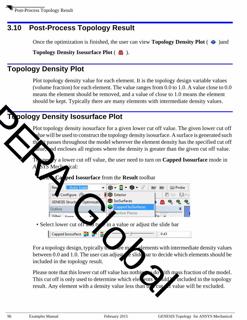
Post-Process Topology Result
PE
3.10 Post-Process Topology Result
Once the optimization is finished, the user can view Topology Density Plot ( )and
Topology Density Isosurface Plot ( ).
Topology Density PlotPlot topology density value for each element. It is the topology design variable values (volume fraction) for each element. The value ranges from 0.0 to 1.0. A value close to 0.0 means the element should be removed, and a value of close to 1.0 means the element should be kept. Typically there are many elements with intermediate density values.
Topology Density Isosurface PlotPlot topology density isosurface for a given lower cut off value. The given lower cut off value will be used to construct the topology density isosurface. A surface is generated such that it passes throughout the model wherever the element density has the specified cut off value, and encloses all regions where the density is greater than the given cut off value.
To specify a lower cut off value, the user need to turn on Capped Isosurface mode in ANSYS Mechanical:
• Select Capped Isosurface from the Result toolbar
• Select lower cut off and type in a value or adjust the slide bar
For a topology design, typically there are many elements with intermediate density values between 0.0 and 1.0. The user can adjust the slide bar to decide which elements should be included in the topology result.
Please note that this lower cut off value has nothing to do with mass fraction of the model. This cut off is only used to determine which elements should be included in the topology result. Any element with a density value less than this cut off value will be excluded.
安世
亚太
RA Global
96 Examples Manual February 2015 GENESIS Topology for ANSYS Mechanical
Estimate Enclosed Volume for Isosurface
PE
3.11 Estimate Enclosed Volume for Isosurface
The user can get an estimated volume fraction enclosed by the isosurface ( ).
First pick a cut off value by viewing the Topology Density Isosurface Plot. Then click on the button shown above, the estimated volume fraction will be printed in the message window. 安
世亚
太 RA Global
GENESIS Topology for ANSYS Mechanical February 2015 Examples Manual 97

Analyze Interpreted Topology Result
PE
3.12 Analyze Interpreted Topology Result
Analyze Interpreted Topology Result ( ) allows the user to analyze an updated FEA model based on an interpretation of the topology result. The analysis is performed using the ANSYS finite element solver. The program, currently, offers two options to interpret topology results.
The first option which is named Polarized Density assigns full density or near zero density to elements that are above or below a user supplied cutoff value (for example 0.4). The second option named Discretized Density assigns discrete density values to group elements that have similar densities.
The first option gives the user a closer idea of what the final structure responses would be. The second option allows to better compare topology results with finite element analysis. Please note that if topology optimization would give perfect 0 or 1 answers, the two methods would give same answers.
A noticeable difference between the two options is that with the first option elements that have low density can be masked out to view the analysis result with only the full density elements shown. This is to simulate the case of removing low density elements from the original model.
The next few paragraphs will describe in more details these two options and show how to use them in the interface.
Option 1: Polarized Density
Element Density CutoffThis option requires the user to specify a cutoff value. This cutoff value is used to construct isosurfaces. The user can decide the cutoff value by viewing Topology Density Isosurface Plot. Typical cutoff values are 0.3 or 0.4.
For the interpreted topology result, the elements that are enclosed by topology density isosurface will be assigned a full density (X=1.0). While elements that are excluded from the topology density isosurface will be assigned a near zero value (X=1.0E-6). The elements passing through the isosurface will be assigned either a full density or a near zero density based on average density values around that element. The equations that define the Power Rule are used to compute a corresponding Young’s Modulus.
With this interpretation option, the elements that are assigned a near zero density represent the elements to be removed from the original FEA model.
安世
亚太
RA Global
98 Examples Manual February 2015 GENESIS Topology for ANSYS Mechanical
Analyze Interpreted Topology Result
PE
Create Named Selection for Polarized ElementsOptionally, the program can generate a named selection for those elements that are assigned a full density. The named selection is called TopologyRegionPolarizedElements.
For a topology density isosurface shown in Figure 3-15, the interpreted topology model with elements that are assigned a full density are shown as pink elements in Figure 3-16.
Figure 3-15Topology Density Isosurface with a cut-off value = 0.45
安世
亚太
RA Global
GENESIS Topology for ANSYS Mechanical February 2015 Examples Manual 99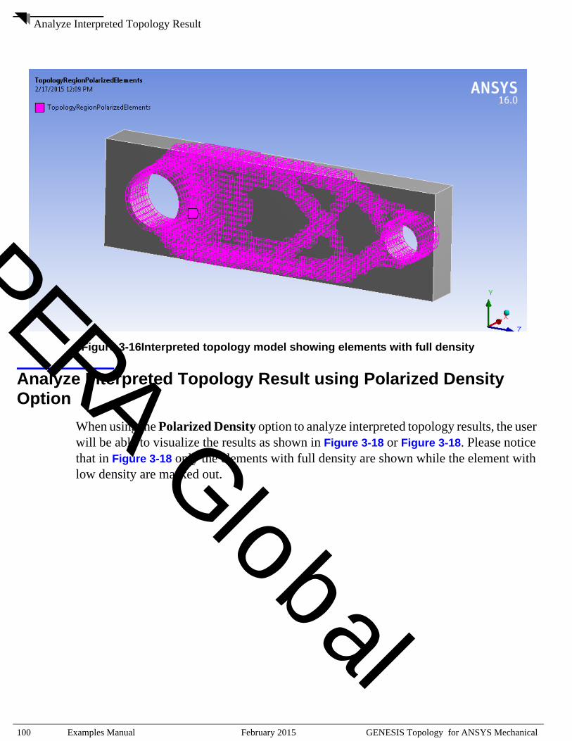
Analyze Interpreted Topology Result
PE
Figure 3-16Interpreted topology model showing elements with full densityAnalyze Interpreted Topology Result using Polarized Density Option
When using the Polarized Density option to analyze interpreted topology results, the user will be able to visualize the results as shown in Figure 3-18 or Figure 3-18. Please notice that in Figure 3-18 only the elements with full density are shown while the element with low density are masked out.
安世
亚太
RA Global
100 Examples Manual February 2015 GENESIS Topology for ANSYS Mechanical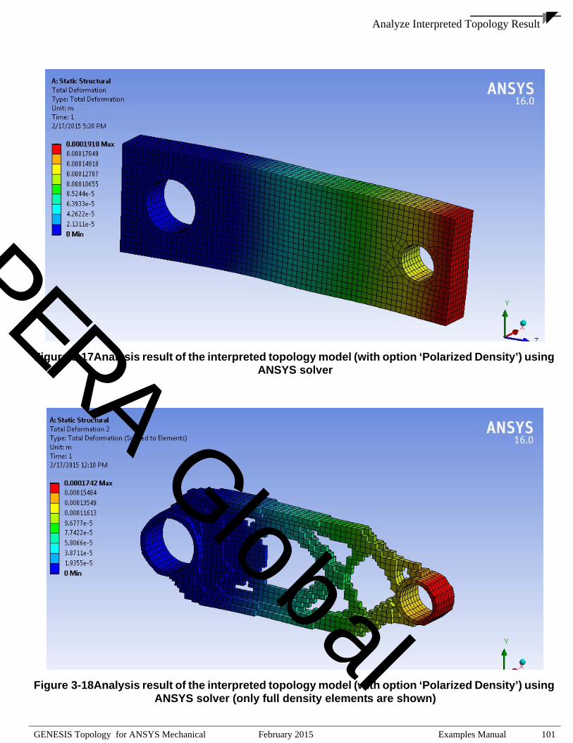
Analyze Interpreted Topology Result
PE
Figure 3-17Analysis result of the interpreted topology model (with option ‘Polarized Density’) usingANSYS solver
Figure 3-18Analysis result of the interpreted topology model (with option ‘Polarized Density’) using ANSYS solver (only full density elements are shown)
安世
亚太
RA Global
GENESIS Topology for ANSYS Mechanical February 2015 Examples Manual 101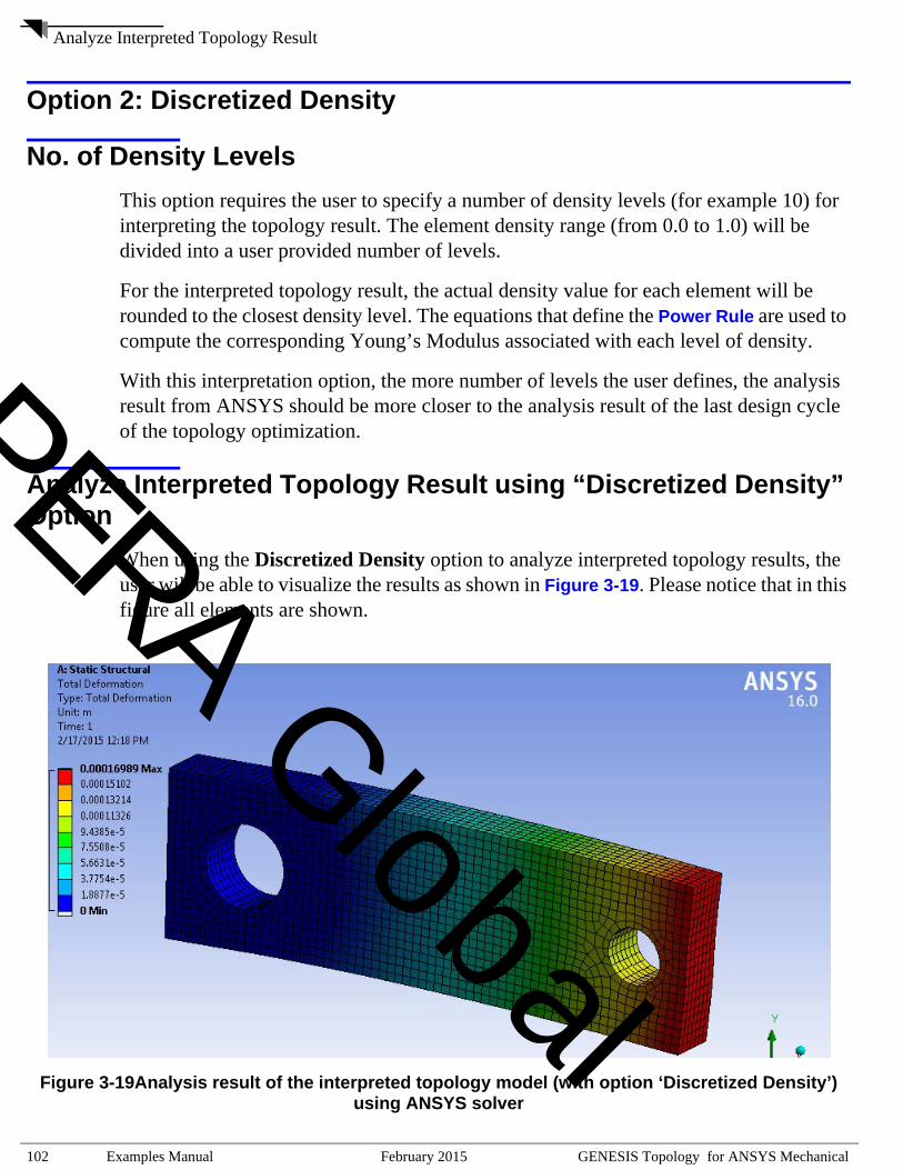
Analyze Interpreted Topology Result
PE
Option 2: Discretized Density
No. of Density LevelsThis option requires the user to specify a number of density levels (for example 10) for interpreting the topology result. The element density range (from 0.0 to 1.0) will be divided into a user provided number of levels.
For the interpreted topology result, the actual density value for each element will be rounded to the closest density level. The equations that define the Power Rule are used to compute the corresponding Young’s Modulus associated with each level of density.
With this interpretation option, the more number of levels the user defines, the analysis result from ANSYS should be more closer to the analysis result of the last design cycle of the topology optimization.
Analyze Interpreted Topology Result using “Discretized Density” Option
When using the Discretized Density option to analyze interpreted topology results, the user will be able to visualize the results as shown in Figure 3-19. Please notice that in this figure all elements are shown.
Figure 3-19Analysis result of the interpreted topology model (with option ‘Discretized Density’) using ANSYS solver
安世
亚太
RA Global
102 Examples Manual February 2015 GENESIS Topology for ANSYS Mechanical
Export Coarsened Surface
PE
3.13 Export Coarsened Surface
The user can export ( ) the optimized structure in a STL/IGES format.
First pick a cut off value by viewing the Topology Density Isosurface Plot. Then set corresponding controls in Analysis Settings −−> Coarsened Surface.安
世亚
太 RA Global
GENESIS Topology for ANSYS Mechanical February 2015 Examples Manual 103
Additional Options
PE
3.14 Additional Options
GENESIS Input Data
Input Data ( ) allows the user to add analysis or design data that is not supported in current version of GENESIS extension.
Data TypeThe data type includes:
• Executive ControlThe executive control portion of the input data is used to control the overall program flow, data checking and diagnostic printing.
• Solution ControlThe solution control portion of the input data is used to set up the various load cases for the design problem.
• Bulk DataBulk data is used to define loads, boundary conditions, elements, properties, materials and design related data. A bulk data entry consist of one or more logical lines.
• Bulk Data DOPTGENESIS input file allows only one DOPT entry. By default, the DOPT entry already exists in the input file exported from GENESIS extension. If the user intends to add any DOPT parameter, this option should be chosen. The input data will be appended to existing DOPT entry.
• Bulk Data Include FileThe user can add bulk data from by including a file.
For details about GENESIS input data format, please refer to GENESIS Analysis Reference Manual and Design Reference Manual.
Number of LinesMaximum of 5 lines are allowed. If the user intends to input more than 5 lines of data, please add another Input Data node or use Bulk Data Include File option.
安世
亚太
RA Global
104 Examples Manual February 2015 GENESIS Topology for ANSYS Mechanical
Additional Options
PE
Write GENESIS Input File and Launch Design Studio
Write GENESIS Input File ( ) option allows the user to write out the input file. The user need to specify the name and location of the input file.
Launch Design Studio ( ) will import user selected GENESIS input file when Launch Design Studio. With this option, the user can access additional functionality in Design Studio.
Once the optimization is solved in Design Studio, the user can post-process the result in Design Studio or bring back the result to ANSYS Mechanical. To bring back the result to ANSYS Mechanical, the user need to switch GENESIS Solver to Dry run to import results in Analysis Settings, and click on Solve.
安世
亚太
RA Global
GENESIS Topology for ANSYS Mechanical February 2015 Examples Manual 105
Recommendations
PE
3.15 Recommendations
Mesh
First Order Element vs. Second Order ElementBy default ANSYS uses second order element when meshing. Second order element gives more accurate analysis result.
However, topology design does not benefit much from second order element if the mesh has a low resolution. It is preferred to have a finer mesh with first order element rather than a coarse mesh with second order element. The reason is that the number of elements (resolution of the mesh) determines the design freedom for topology design since topology will create design variables associated with elements in the mesh.
UniformA uniform mesh is also preferred for topology designed region. The user should check the mesh quality for interior of the model using the cut view in ANSYS Mechanical.
安世
亚太
RA Global
106 Examples Manual February 2015 GENESIS Topology for ANSYS Mechanical
PE
P3⁄STRUCTURAL OPTIMIZATION (Vol. II)
CHAPTER 4Appendix
o Appendix A: Features Support in Current Version
o Appendix B: Conversion Mapping
安世
亚太
RA Global

PE
4.1 Appendix A: Features Support in Current Version
Table 1: Functional Modules
Category GENESIS GENESIS Topology for ANSYS Mechanical
Structural Optimization
Topology Yes Yes
Sizing Yes No
Shape Yes No
Topography Yes No
Topometry Yes No
Freeform Yes No
Special Features Matching Yes No
Mode Tracking Yes Yes
Manufacture Constraints Yes Yes
Table 2: Topology Design
Category GENESIS GENESIS Topology for ANSYS Mechanical
Designable Element Solid Yes Yes
Shell Yes Yes
Bar Yes No
Rod Yes No
Beam Yes Yes
Weld Yes No
Shear Yes No
Axisymmetric Yes No
Loading Condition Static Yes Yes
Eigenvalue (Modal) Yes Yes
Buckling Yes Yes
Frequency Response Yes Yes
Random Response Yes Yes
安世
亚太
RA Global
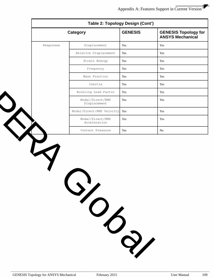
Appendix A: Features Support in Current Version
PE
Table 2: Topology Design (Cont’)
Category GENESIS GENESIS Topology for ANSYS Mechanical
Responses Displacement Yes Yes
Relative Displacement Yes Yes
Strain Energy Yes Yes
Frequency Yes Yes
Mass Fraction Yes Yes
Inertia Yes Yes
Buckling Load Factor Yes Yes
Modal/Direct/RMS Displacement
Yes Yes
Modal/Direct/RMS Velocity Yes Yes
Modal/Direct/RMS Acceleration
Yes Yes
Contact Pressure Yes No
安世
亚太
RA Global
GENESIS Topology for ANSYS Mechanical February 2015 User Manual 109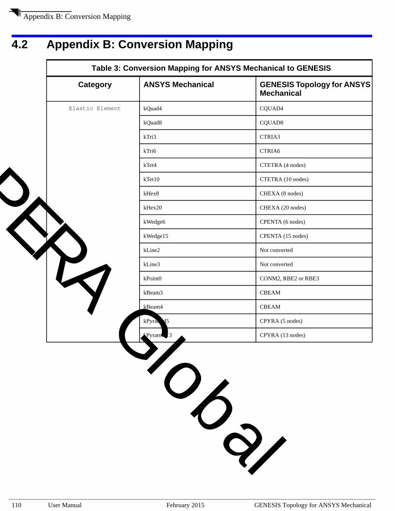
Appendix B: Conversion Mapping
PE
4.2 Appendix B: Conversion Mapping
Table 3: Conversion Mapping for ANSYS Mechanical to GENESIS
Category ANSYS Mechanical GENESIS Topology for ANSYS Mechanical
Elastic Element kQuad4 CQUAD4
kQuad8 CQUAD8
kTri3 CTRIA3
kTri6 CTRIA6
kTet4 CTETRA (4 nodes)
kTet10 CTETRA (10 nodes)
kHex8 CHEXA (8 nodes)
kHex20 CHEXA (20 nodes)
kWedge6 CPENTA (6 nodes)
kWedge15 CPENTA (15 nodes)
kLine2 Not converted
kLine3 Not converted
kPoint0 CONM2, RBE2 or RBE3
kBeam3 CBEAM
kBeam4 CBEAM
kPyramid5 CPYRA (5 nodes)
kPyramid13 CPYRA (13 nodes)
安世
亚太
RA Global
110 User Manual February 2015 GENESIS Topology for ANSYS Mechanical
Appendix B: Conversion Mapping
PE
Load Force FORCE, PLOAD4, PLOAD5
Moment MOMENT
Pressure PLOAD4, PLOAD5
Bearing Load FORCE, PLOAD4, PLOAD5
Joint Load FORCE,SPCD,MPC
Bolt Pretension FORCE,SPCD,MPC
Gravity GRAV
Acceleration GRAV
Rotational Velocity RFORCE
Thermal Conditions TEMP
Modal EIGR
Buckling EIGR, STATSUB
Table 3: Conversion Mapping for ANSYS Mechanical to GENESIS (Cont’)
Category ANSYS Mechanical GENESIS Topology for ANSYS Mechanical
Boundary Conditions Fixed support SPC
Simple support SPC
Frictionless support SPC
Fixed rotation SPC
Cylinder support SPC
Displacement SPC
Constraint Equations MPC
Remote Boundary Conditions
Remote Force FORCE, RBE2 or RBE3
Remote Displacement SPC, RBE2 or RBE3
Point Mass CONM2, RBE2 or RBE3
Remote Point RBE2 or RBE3
Table 3: Conversion Mapping for ANSYS Mechanical to GENESIS
安世
亚太
RA Global
GENESIS Topology for ANSYS Mechanical February 2015 User Manual 111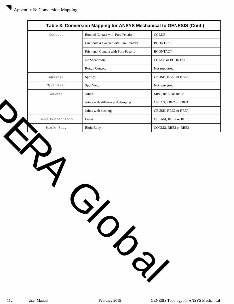
Appendix B: Conversion Mapping
PE
Contact Bonded Contact with Pure Penalty CGLUE
Frictionless Contact with Pure Penalty BCONTACT
Frictional Contact with Pure Penalty BCONTACT
No Separation CGLUE or BCONTACT
Rough Contact Not supported
Springs Springs CBUSH, RBE2 or RBE3
Spot Weld Spot Weld Not converted
Joints Joints MPC, RBE2 or RBE3
Joints with stiffness and damping CELAS, RBE2 or RBE3
Joints with bushing CBUSH, RBE2 or RBE3
Beam Connections Beam CBEAM, RBE2 or RBE3
Rigid Body Rigid Body CONM2, RBE2 or RBE3
Table 3: Conversion Mapping for ANSYS Mechanical to GENESIS (Cont’)
安世
亚太
RA Global
112 User Manual February 2015 GENESIS Topology for ANSYS Mechanical