user’s manual for the navy coastal ocean model (ncom ... · user’s manual for the navy coastal...
TRANSCRIPT

Naval Research LaboratoryStennis Space Center, MS 39529-5004
NRL/MR/7320--09-9151
Approved for public release; distribution is unlimited.
User’s Manual for theNavy Coastal Ocean Model (NCOM)Version 4.0Paul J. Martin Charlie n. Barron luCy F. SMedStad tiMothy J. CaMPBell alan J. WallCraFt roBert C. rhodeS Clark roWley taMara l. toWnSend
Ocean Dynamics and Prediction Branch Oceanography Division
February 6, 2009
Suzanne n. Carroll
Planning Systems, Inc. Stennis Space Center, Mississippi

i
REPORT DOCUMENTATION PAGE Form ApprovedOMB No. 0704-0188
3. DATES COVERED (From - To)
Standard Form 298 (Rev. 8-98)Prescribed by ANSI Std. Z39.18
Public reporting burden for this collection of information is estimated to average 1 hour per response, including the time for reviewing instructions, searching existing data sources, gathering and maintaining the data needed, and completing and reviewing this collection of information. Send comments regarding this burden estimate or any other aspect of this collection of information, including suggestions for reducing this burden to Department of Defense, Washington Headquarters Services, Directorate for Information Operations and Reports (0704-0188), 1215 Jefferson Davis Highway, Suite 1204, Arlington, VA 22202-4302. Respondents should be aware that notwithstanding any other provision of law, no person shall be subject to any penalty for failing to comply with a collection of information if it does not display a currently valid OMB control number. PLEASE DO NOT RETURN YOUR FORM TO THE ABOVE ADDRESS.
5a. CONTRACT NUMBER
5b. GRANT NUMBER
5c. PROGRAM ELEMENT NUMBER
5d. PROJECT NUMBER
5e. TASK NUMBER
5f. WORK UNIT NUMBER
2. REPORT TYPE1. REPORT DATE (DD-MM-YYYY)
4. TITLE AND SUBTITLE
6. AUTHOR(S)
8. PERFORMING ORGANIZATION REPORT NUMBER
7. PERFORMING ORGANIZATION NAME(S) AND ADDRESS(ES)
10. SPONSOR / MONITOR’S ACRONYM(S)9. SPONSORING / MONITORING AGENCY NAME(S) AND ADDRESS(ES)
11. SPONSOR / MONITOR’S REPORT NUMBER(S)
12. DISTRIBUTION / AVAILABILITY STATEMENT
13. SUPPLEMENTARY NOTES
14. ABSTRACT
15. SUBJECT TERMS
16. SECURITY CLASSIFICATION OF:
a. REPORT
19a. NAME OF RESPONSIBLE PERSON
19b. TELEPHONE NUMBER (include areacode)
b. ABSTRACT c. THIS PAGE
18. NUMBEROF PAGES
17. LIMITATIONOF ABSTRACT
User’s Manual for the Navy Coastal Ocean Model (NCOM) Version 4.0
Paul J. Martin, Charlie N. Barron, Lucy F. Smedstad, Timothy J. Campbell, Alan J. Wallcraft, Robert C. Rhodes, Clark Rowley, Tamara L. Townsend, and Suzanne N. Carroll*
Naval Research LaboratoryOceanography DivisionStennis Space Center, MS 39529-5004 NRL/MR/7320--09-9151
Approved for public release; distribution is unlimited.
Unclassified Unclassified UnclassifiedUL 73
Lucy F. Smedstad
(228) 688-5365
The version 4 series of the Navy Coastal Ocean Model (NCOM) has been developed at the Naval Research Laboratory (NRL) and transitioned to the Navy Oceanographic Office. New capabilities include a general vertical coordinate (GVC) option in addition to the sigma-z coordinate vertical grid, Earth System Modeling Framework (ESMF) compliance, and several other compile time options that increase the flexibility of the model code. NRL has also begun maintaining NCOM in version control using a Subversion repository. This User’s Manual documents the setup and execution of the NCOM version 4.0 series.
06-02-2009 Memorandum Report
Space & Naval Warfare Systems Command2451 Crystal DriveArlington, VA 22245-5200
73-5091-18-9
SPAWAR
0603207N
Global ocean modelingCoastal modeling
ESMFOperational
NCOMSVN
*Planning Systems, Inc., Stennis Space Center, MS 39529

Table of Contents TABLE OF CONTENTS................................................................................................................................iii
TABLE OF FIGURES AND TABLES.......................................................................................................... V
1.0 INTRODUCTION.............................................................................................................................. 1
2.0 APPLICATION.................................................................................................................................. 3 2.1 DESCRIPTION OF NCOM USAGE ...................................................................................................... 3 2.2 MAIN DIRECTORY STRUCTURE ........................................................................................................ 3 2.3 RUNNING ENVIRONMENT ............................................................................................................... 10 2.4 CODE MODIFICATIONS ................................................................................................................... 10
2.4.1 Changes from NCOM 2.6 to NCOM 4.0 (12-26-2007) ............................................................ 10 2.4.2 NCOM Subversion Repository.................................................................................................. 10
3.0 LIMITATIONS AND ASSUMPTIONS......................................................................................... 12 3.1 NCOM TESTING: A NOTE TO USERS.............................................................................................. 13
4.0 OPERATING GUIDELINES ......................................................................................................... 14 4.1 MAKING THE NCOM EXECUTABLE: ..................................................................................................... 16
4.1.1 Setting/Checking Parameters ................................................................................................... 16 4.1.2 NCOM Build Information......................................................................................................... 16
4.1.2.1 Required Build Variables.............................................................................................................. 16 4.1.2.2 Optional Build Variables .............................................................................................................. 17
4.1.3 Set Halo Width.......................................................................................................................... 19 4.1.4 Set Maximum Dimensions ........................................................................................................ 19 4.1.5 Set Macro Values...................................................................................................................... 19 4.1.6 Create Executable File ............................................................................................................. 19 4.1.7 Deleting Executables and Libraries ......................................................................................... 20
4.2 SETTING UP A SIMULATION............................................................................................................ 20 4.3 RUNNING A SIMULATION................................................................................................................ 21 4.4 MODEL INPUT FILES....................................................................................................................... 22 4.5 MODEL OUTPUT FILES ................................................................................................................... 25 4.6 INPUT PARAMETERS IN FILE OPARM_1.D. ................................................................................... 25 4.7 PARAMETERS IN FILE PARAM.H .................................................................................................... 38 4.8 PARAMETERS IN FILE MACROS.H .................................................................................................. 39 4.9 COAMPS NAMELIST PARAMETERS FILES ..................................................................................... 40 4.10 INTERACTIVE PRINTING AND PLOTTING ......................................................................................... 43 4.11 DOING A MODEL RESTART............................................................................................................. 44 4.12 CHECKING FOR BIT-FOR-BIT REPRODUCIBILITY OF MODEL RESULTS .......................................... 44 4.13 USING HIGHER-ORDER FINITE DIFFERENCES.................................................................................. 44 4.14 USING NESTED GRIDS .................................................................................................................... 46 4.15 RUNNING NCOM WITH TIDES........................................................................................................ 48 4.16 HORIZONTAL AND VERTICAL GRID LAYOUT AND INDEXING ........................................................ 49 4.17 INDEXING OF OPEN BOUNDARY POINTS ......................................................................................... 50 4.18 TROUBLESHOOTING NCOM........................................................................................................... 53
4.18.1 The NCOM run has immediately crashed............................................................................ 53 4.18.2 Model runs fine for a time and then suddenly crashes ....................................................... 53 4.18.3 The model returned strange results ..................................................................................... 53 4.18.4 Spuriously low or high T or S values.................................................................................. 53 4.18.5 General 2*dx Noise ............................................................................................................ 54 4.18.6 Spurious circulation around topographic features............................................................. 55
5.0 FUNCTIONAL DESCRIPTION .................................................................................................... 56
iii

6.0 TECHNICAL REFERENCES........................................................................................................ 56 6.1 NCOM SOFTWARE DOCUMENTATION ........................................................................................... 56 6.2 GENERAL TECHNICAL REFERENCES ............................................................................................... 56 6.3 RECOMMENDED READING.............................................................................................................. 57
7.0 NOTES .............................................................................................................................................. 58 7.1 ACRONYMS AND ABBREVIATIONS.................................................................................................. 58
APPENDIX A: NCOM CODE VARIABLES.............................................................................................. 60 PRIMARY NCOM VARIABLES ...................................................................................................................... 60
Main Input Dimensions........................................................................................................................... 60 Halo width and maximum dimensions .................................................................................................... 60 Time variables......................................................................................................................................... 61 Grid indexing variables .......................................................................................................................... 61 Time indexing variables.......................................................................................................................... 61 Grid related variables............................................................................................................................. 62 Input values for vertical grid .................................................................................................................. 62 Input values for horizontal grid .............................................................................................................. 62 Main prognostic variables ...................................................................................................................... 62 Variables used for relaxation of T and S to specified values.................................................................. 63 Surface forcing variables........................................................................................................................ 63 Open boundary variables........................................................................................................................ 63 River inflow variables ............................................................................................................................. 64 Other variables ....................................................................................................................................... 64 Temporary variables............................................................................................................................... 65
CONSTANTS.................................................................................................................................................. 66 Defined and Calculated Constants ......................................................................................................... 66 Defined Constants................................................................................................................................... 66 Calculated Constants .............................................................................................................................. 67 Calculated Grid Related Constants ........................................................................................................ 67
iv

v
Table of Figures and Tables
FIGURE 4.0-1: FLOW DIAGRAM DESCRIBING THE EXECUTION OF THE NCOM................................................... 15 TABLE 4.4-1: NCOM LIST AND DESCRIPTION OF INPUT FILES............................................................................ 23 TABLE 4.5-1: OUTPUT FILES............................................................................................................................. 25 TABLE 4.6-1: RUN CONTROL PARAMETERS (RUNO) .......................................................................................... 26 TABLE 4.6-2: OUTPUT CONTROL PARAMETERS (OUTO) .................................................................................... 26 TABLE 4.6-3: OUTPUT CONTROL PARAMETERS FOR SURFACE FIELDS (IOUTO) ................................................. 27 TABLE 4.6-4: OUTPUT CONTROL PARAMETERS FOR 3D FIELDS OUTPUT FILE (IOUTO) ..................................... 27 TABLE 4.6-5: PHYSICAL OPTIONS (PHYO) ......................................................................................................... 28 TABLE 4.6-6: PHYSICAL PARAMETERS (PHYP) ................................................................................................... 30 TABLE 4.6-7: NUMERICAL OPTIONS (NUMO) ..................................................................................................... 31 TABLE 4.6-8: NUMERICAL PARAMETERS (RNUMO)............................................................................................ 32 TABLE 4.6-9: SURFACE FORCING OPTIONS AND PARAMETERS (ISBCO, LSBCO, SBCO) ...................................... 33 TABLE 4.6-10: LATERAL BOUNDARY OPTIONS (IOBCO).................................................................................... 35 TABLE 4.6-11: LATERAL BOUNDARY PARAMETERS (OBCO) .............................................................................. 37 TABLE 4.6-12: RIVER INFLOW PARAMETERS (RIVO) ......................................................................................... 37 TABLE 4.6-13: GRID NESTING PARAMETERS (NSTO) ......................................................................................... 38 TABLE 4.6-14: DIAGNOSTICS PARAMETERS (DIAGO)......................................................................................... 38 TABLE 4.7-1: PARAMETERS LISTED IN PARAM.H. ............................................................................................. 38 TABLE 4.8-1: USER-DEFINED MACROS OF MACROS.H...................................................................................... 39 TABLE 4.9-1: COAMPS NAMELIST PARAMETERS (OMNL.H) ............................................................................ 40 TABLE 4.9-2: COAMPS OMNLOFF PARAMETERS (OMNLOFF.H) .................................................................... 42 TABLE 4.9-3: COAMPS ATMOSPHERIC AND OCEAN PARAMETERS (DSETNL.H) ............................................... 42 TABLE 4.9-4: COAMPS PARAMETERS (COAMPS_PARMS.H) .............................................................................. 43 FIGURE 4.16-1: OPEN BOUNDARY ARRAY INDEXING EXAMPLE. ........................................................................ 51

NRL/MR/7320--08-9151 NCOM Version 4.0 User’s Manual
1.0 Introduction The Navy Coastal Ocean Model (NCOM) Version 4.0 is based primarily on two existing ocean circulation models, the Princeton Ocean Model (POM) (Blumberg and Mellor 1983; Blumberg and Mellor 1987) and the Sigma/Z-level Model (SZM) (Martin et al., 1998). NCOM Version 4.0 has a free-surface and is based on the primitive equations and the hydrostatic, Boussinesq, and incompressible approximations. The Mellor Yamada Level 2 (MYL2) and MYL2.5 turbulence models are provided for the parameterization of vertical mixing. The vertical mixing enhancement scheme of Large et al. (1994) is also offered for parameterization of unresolved mixing processes occurring at near-critical Richardson numbers. The inclusion of a source term in the model equations allows for the input of river and runoff inflows. The model uses a staggered Arakawa C grid (as in POM). Spatial finite differences are mostly second-order centered (as in POM), but there are options to use higher-order spatial differences for some terms. The temporal scheme is leapfrog, with an Asselin filter to suppress timesplitting (as in POM). Most terms are treated explicitly in time, but the propagation of surface waves and vertical diffusion are treated implicitly. The horizontal grid is orthogonal-curvilinear (as in POM). NCOM 4.0 has two choices of vertical grid, which are selected at compile time. One choice is the original vertical grid used by NCOM, which is a hybrid sigma and z-level grid with sigma coordinates used from the surface down to a specified depth and level coordinates used below the specified depth. The switch from sigma to level coordinates can occur at any specified interface between layers, i.e., from just below the uppermost layer (there must be at least one sigma layer at the surface) to the bottom of the lowest layer (in which case the entire grid would be sigma coordinate, as in POM). On the sigma coordinate portion of the grid, each sigma layer is a fixed fraction of the depth from the surface to the bottom of the sigma coordinate grid. This fractional depth may vary for different sigma layers, but cannot change within a particular layer. On the level portion of the grid, each layer's depth and thickness is fixed and the bottom depth is adjusted to match the depth of the nearest layer. The second, newer, choice of vertical grid is a general vertical coordinate (GVC) grid. The GVC grid consists of a three-tiered vertical grid structure comprised of: (1) a "free" sigma grid near the surface that expands and contracts with the movement of the free surface, (2) a "fixed" sigma grid that does not move with the free surface, and (3) a z-level grid that allows for "partial" bottom cells. For both the "free" and "fixed" sigma grids, the fractional layer thickness can be specified independently for each grid cell and the land-sea masking can be different for different sigma layers. The vertical grid structure can consist of just (1), or (1) and (2), or (1) and (3), or (1), (2), and (3). This new vertical grid structure allows for more flexibility on both the sigma and z-level portions of the grid. For the sigma grid, the fractional layer thickness can vary both horizontally and vertically (i.e., it can be specified independently at each model grid pt) and masking can be used on the sigma grid to mask land areas and reduce the number of active sigma layers. For the z-level grid, grid cells at the bottom can be made "partial" cells so that the z-level grid can
1
_______________
Manuscript approved December 29, 2008.

NRL/MR/7320--08-9151 NCOM Version 4.0 User’s Manual
match the true bottom depth. In addition, a "fixed" sigma grid that does not expand and contract with the movement of the free surface can be used between the "free" sigma grid near the surface and the (fixed) z-level grid. However, the increased flexibility of the generalized vertical grid comes at the cost of a 15-20% increase in the required memory storage and CPU time. Also, the use of “partial” z-level cells involves increased numerical truncation error because of the abrupt change in grid-layer thickness at a "partial" grid cell. The “classic” sigma grid, where each layer is a fixed fraction of the total depth of the sigma grid, has some numerical advantages over the generalized sigma grid. The NCOM surface boundary conditions are the surface stress for the momentum equations, the surface heat flux for the temperature equation, and the effective surface salt flux for the salinity equation. The bottom boundary conditions are the bottom drag for the momentum equations, which is parameterized by a quadratic drag law, and zero flux for the temperature and salinity equations. NCOM provides for an arbitrary number of levels of nesting. This nesting capability is made possible by using dynamic memory allocation with array dimensions specified at run time and by passing model variables to subroutines through subroutine argument lists rather than through common blocks. This allows the same model routines to calculate the different nests.
2

NRL/MR/7320--08-9151 NCOM Version 4.0 User’s Manual
2.0 Application 2.1 Description of NCOM Usage This manual describes the procedures for running the Navy Coastal Ocean Model Version 4.0 (NCOM). NCOM is set up so that the main model program requires little or no alteration to run a particular simulation, as almost everything needed for a model simulation is passed in via input files. A setup program is required to generate the input files for regional NCOM domains. It is recommended that the user modify one of the existing setup programs that are available. Most of the model input files are read and written by the subroutines in file ncom1rwio.F. The same subroutine is usually used to read and write a particular file so that the code for reading and writing the file is in the same place and the read and write instructions can more easily be kept consistent. Therefore, most of the subroutines in file ncom1rwio.F have an initial parameter that is either set to 1 to read or 2 to write the file. A separate technical manual, the Software Design Description (SDD), complements this document and contains the code of the model as well as flow charts and descriptions of the programs and sub-programs (Martin et al., 2008). The physics and basic equations may be found in Barron et al., 2006. This User’s Manual, along with the SDD and the Validation Test Reports (Barron et al., 2007, 2008) form a comprehensive documentation package for the NCOM 4.0 delivery. A User’s Guide for the global NCOM nowcast/forecast model, called the Global Ocean Forecast System (GOFS), is also available (Smedstad et al., 2008). 2.2 Main Directory Structure The directory structure for operational use of the system consists of directories for (1) the model code(s) and (2) individual simulations. The model code directory (ncom_4.0) contains all the files needed to generate the NCOM executable. The typical structure of this directory is:
ncom_4.0/ Makefile.ncom Top-level Makefile for NCOM.
Makefile - Secondary- level Makefile for NCOM. README.txt Compiling and running a simulation. README.make NCOM build information. bin/- Directory for NCOM executable(s). The executables are placed in
subdirectories that follow the naming convention described in Section 4.1.2.
config/- Configuration and makefile fragments used for compiling NCOM code. Each makefile fragment is set up for some combination of a
3

NRL/MR/7320--08-9151 NCOM Version 4.0 User’s Manual
(i) specific machine architecture (NCOM_ARCH) (ii) compiler (NCOM_COMP), and (iii) user-specific (NCOM_USER) options.
doc/- Directory of Readme documentation/explanation files. ncom_changes.txt List of NCOM errors and changes. ncom_guide.txt User’s guide for NCOM 4.0 README.version- Description of NCOM version number
string. README.<xxx> Symbolic link to specific README
on <xxx>. include/- NCOM include files that are included via cpp (These are now
using suffix *.h rather than *.inc). CAF.h- Co-Array Fortran I/O.
COAMPS.h- Common block to store info about ocean/atm model grid for COAMPS.
COAMPS_parms.h COAMPS parameter include file. COMMON.h- Common blocks for NCOM.
Dsetnl.h- COAMPS directory path include file. HEADER_MPI.h- MPI header on generic machine. HEADER_MPI_AIX.h- MPI header on IBM SP. HEADER_MPI_T3E.h- MPI header on Cray T3E. MACROS.h- Macros for customizing NCOM. NCOMPAR.h- Common blocks for NCOM
subroutine OMODEL. Omnl.h and omnloff.h- COAMPS ocean model namelist
include files. PARAM.h- Compile-time constants for NCOM.
README.include- Help file for includes. README.macros- Help file for macros in MACROS.h.
lib/- Directory of NCOM compiled libraries- Libraries are placed in subdirectories that follow the naming convention described in Section 4.1.2.
sigz.global/- libncom.a - Compiled library of all NCOM
subroutines. libncom_setup.a - Compiled library of all NCOM setup
subroutines. libsrc/- Directory of all NCOM Fortran subroutine files.
Makefile- Makes compiled libraries containing collections of NCOM Fortran files and puts libraries on lib/ directory.
cdf/- Contains a set of netCDF specific subroutines.
4

NRL/MR/7320--08-9151 NCOM Version 4.0 User’s Manual
coampslib/- Subroutines for working with COAMPS fields. Makefile- Makefile to compile local source code. datar.F- Reads COAMPS-style flat files. datar_new.F- Reads COAMPS-style flat files. dataw.F- Writes COAMPS-style flat files. dataw_new.F- Writes COAMPS-style flat files. dfalts.F- Returns information about the specified-input
field name, e.g., default contour interval, max/min color shading bar values.
grdcon.F- Calculates the grid constant for input grid projection and grid parameters.
grdij.F- Generates real grid index values. ij2ll.F- Computes lat/lon from real grid index values
for specified grid projection and parameters. ll2ij.F- Computes real grid index coordinates from
lat/lon values for specified grid projection and parameters.
rdata.F- Gets information for specified input field. rotang.F- Calculates angle of grid with respect to local
lat/lon for specified grid. s2hms.F- Converts from s to hour, min, sec. slen.F- Gives the size of a character string. uvg2uv.F- Converts grid u/v to earth-oriented u/v, i.e.,
with u directed eastward and v directed northward.
wdata.F - Writes data field to COAMPS-style flat file. esmf/- Directory of ESMF routines. Makefile- Makefile to compile local source code. ncom1esmf.F- NCOM ESMF Module. fnoclib/- Directory of main FNMOC routines and
include files. Makefile- Makefile to compile local source code. bessel.F- General 2D bessel interpolation. cctop.F- Converts fields from vector to Polar
(magnitude and direction) form. ch2int.F- Gets integer numerical value from integer
character string. dfuv.F- Converts vectors from earth-oriented
direction and magnitude to u/v form on a conic grid projection.
differs.F- Perform operations performed on two input fields depending on value of input flag.
5

NRL/MR/7320--08-9151 NCOM Version 4.0 User’s Manual
dtgchk.F- Checks if DTG is valid. dtgdif.F- Returns difference in hours of two input
DTGs. dtgmod.F- Returns new DTG given base DTG and
increment in hours. dtgnum.F- Given DTG, returns integer values of year,
month, day, hour, days into the year, and hours into the year.
dtgops.F- Returns three types of DTG. edge.F- Performs next-to-edge processing for low-
pass filter. fintrp.F- Interpolates input field values. gcpnts.F- Computes evenly spaced lat/lon points along
a great circle path between two input lat/lon locations.
gent.F- Gets a single entry from a HRLS table. getls.F- Reads a HRLS table from ISIS or UNIX files.
imaxcv.F- Computes imax from colcnt and rowcnt. int2ch.F- Converts an integer to an left-justified
character string. ioinq.F- Uses Fortran “Inquire” statement to give info
for user in tracking the action of the program I/O.
isint.F- Tests if a character string contains only digits and a possible sign.
jmaxcv.F- Computes jmax from colcnt and rowcnt, depending on stordsc.
leapyr.F- Checks to see if input year is a leap year. lndavg.F- Computes values for flagged pts in a 2D field
as averages of surrounding non-flagged pts. lpf.F- Low-pass 2D filter. niddf.F- Computes the value of variables, given 1D
arrays and independent variables. ocord.F- Reads file containing instructions for
outputting model fields in flat file format. pctocc.F- Converts vector fields from dir and mag to
u/v form. qprint.F- Quick prints parts of a gridded field. rlpnts.F- Computes grid index locations of evenly-
spaced x/y pts along a straight line on the grid.
6
NRL/MR/7320--08-9151 NCOM Version 4.0 User’s Manual
strcmpr.F- Tests to see that two char strings match, disregarding whether letters are upper or lower case.
strleft.F- Deletes leading white space from a char string, left-justifying the string.
strlen.F- Computes the length of an input string. strnot.F- Finds the first location in an input string that
is not a blank. strpars.F- Extracts substrings from a char string. unstrgr.F- Unstaggers a staggered gridded field. uvdf.F- Converts from u/v on a conic grid to earth-
oriented speed and direction. misc/- Directory of miscellaneous NCOM subroutines. Makefile- Makefile to compile local source code. allocate.F- Allocates the no. of array elements needed. cubspl_irr.F- Cubic spline interp. for irregular output grid. gc_ellipsoid.F-Returns distances in m, azimuth angle in deg. ocubspl_irr.F- Old cubic spline interp. for irreg. output grid. padarr.F- Embeds model horiz. grid into comp. horiz.
grid. tablk2s.F- Interpolates value from 2D array using linear
interp. timesubs.F- Time subroutines. w_ncomnc.F- Writes NCOM data into a netCDF file. w_ncomnc2.F-Writes NCOM data into a netCDF file. w_rgb.F- Converts real array f to an output rgb file. ncom/- Directory of NCOM main Fortran subroutines.
Makefile- Makefile to compile local source code. ncom1.F- Routines to set up memory for NCOM and
integrate the ocean model in time(except for driver module, which is in file ncom.F in directory src/ncom/.
ncom1baro.F- Routines to update free-surface. ncom1coam.F-Routines to get surface air-sea flux fields
from COAMPS atmospheric model flat file output.
ncom1fct_gvc.F- Routines for advection of scalar fields using FCT to avoid advective overshoots- GVC grid.
ncom1fct_sigz.F- Routines for advection of scalar fields using FCT-sig-z grid.
7

NRL/MR/7320--08-9151 NCOM Version 4.0 User’s Manual
ncom1init_gvc.F-Routines to initialize ocean model-GVC grid.
ncom1init_sigz.F-Routines to initialize ocean model-sig-z grid.
ncom1nest2.F-Routines to interpolates boundary conditions for and provide feedback from nested grids.
ncom1obc_gvc.F-Routines to handle OBCs-GVC grid. ncom1obc_sigz.F- Routines to handle OBCs -sig-z grid. ncom1out_gvc.F-Routines to output model results- GVC
grid. ncom1out_sigz.F- Routines to output model results -sig-z
grid. ncom1plib.F- Generic routines from Paul Martin's library
plib. ncom1rwio.F- Routines to read/write I/O files. ncom1sbc.F- Routines to obtain surface forcing. ncom1tide.F- Routines to provide tidal forcing. ncom1updt_gvc.F- Main update routines for u, v, T, S- GVC
grid. ncom1updt_sigz.F- Main update routines for u, v, T, S-sig-z
grid. ncom1util.F- Utility routines used for testing, etc.
ncom1vmix_gvc.F-Routines to compute vertical mixing-GVC grid.
ncom1vmix_sigz.F- Routines to compute vertical mixing-sig-z grid.
pdum/- Directory for dummy NCOM routines, e.g., plotting. Makefile – Makefile to compile local source code. ncom1pdum.F-Dummy plotting routines for NCOM when
interactive NCAR graphics are not available. r10k/- Fortran routines specific to SGI Origin 2000.
Makefile - Makefile to compile local source code. wtime.c- NCOM routine to calculate wall time on
SGIs. zunder.c- NCOM routine to flush underflows to zero on
SGIs. setup/- General routines to support setting up a simulation and post
process output. Makefile - Makefile to compile local source code. ncom_setup_plib_gvc.F-General routines for setting up a
simulation-GVC grid.
8
NRL/MR/7320--08-9151 NCOM Version 4.0 User’s Manual
ncom_setup_plib_sigz.F-General routines for setting up a simulation-sig-z grid.
ncom_setup_spln.F- Spline interpolation routines from D. S. Ko.
sunw/- Fortran routines specific to Sun Ultra 2 workstations. Makefile - Makefile to compile local source code. wtime.c- NCOM routine to calculate wall time on Sun
systems. util/- Directory of communication routines for shared memory
(SM) and multi-processor (MP) computing. Makefile- Makefile to compile local source code.
README.xmc- Brief descriptions of all communication routines.
README.za- Brief descriptions of machine-specific routines.
xmc.F- Select between xmc_mp.F and xmc_sm.F. xmc_mp.F- Communication routines for multiple
processors. xmc_sm.F- Communication routines for shared memory
computer. za.F- Select between za_mp.F and za_sm.F. za_mp.F- I/O routines for multiple processors. za_sm.F- I/O routines for shared memory computer.
mod/- Directory of compiled NCOM Fortran modules. The modules are placed in subdirectories that follow the naming convention described in Section 4.1.2.
sigz.global/- Contains compiled global NCOM Fortran modules. src/- Makefile-
esmf/- ncom.F- ESMF driver for stand-alone NCOM.
ncom/-Directory for NCOM driver and makefile to make the executable.
Makefile - Compile ncom.F, link executable and put on /bin. ncom.F - Main driver routine for NCOM.
test_xca/- Makefile- Makefile to build program test_xca.F. test_xca.F- Program to test xctilr. test_xcl/- Makefile- Makefile to build program test_xcl.F. test_xcl.F- Program to test xclget and xclg3d.
9

NRL/MR/7320--08-9151 NCOM Version 4.0 User’s Manual
2.3 Running Environment The input/output files are either IEEE binary or ASCII files and should be fully portable to the different computers that are normally used (Sun, SGI, Cray XT, IBM-SP, DecAlpha). Requirements to "run" a simulation are limited to the model executable, the model run script, and the model input files. Hence, it may be convenient to set up the input files and look at the model output on a computer separate from the one on which the model itself is being run (e.g., where interactive plotting is available to make it easier to inspect the fields). 2.4 Code Modifications Several code modifications have been made from the original NCOM Version 1.0. For a complete history of all code changes made, refer to ncom_guide.txt in the \ncom\4.0\doc folder. 2.4.1 Changes from NCOM 2.6 to NCOM 4.0 (12-26-2007)
• Merged 2.6 (sigma-z) and 3.4 (GVC) versions into single version. This change only affects libsrc/ncom, libsrc/setup and the build system.
• A new C-preprocessor macro called "GVC" is used to select the sigma-z code or the GVC code at compile time. The user input build variable NCOM_VERT (=sigz or =gvc) is used to determine the type of build. The default is NCOM_VERT=sigz.
• The name of the subdirectories for executables, libraries and modules is modified to include the NCOM_VERT string.
• Source files particular to the type of vertical coordinate system have either "_sigz" or "_gvc" added to the name of the file.
• Other source files that have subroutines dependent on the coordinate system choice use the GVC C-preprocessor macro to enable the correct subroutines.
• The top level module (libsrc/ncom/ncom1.F) uses the GVC C-preprocessor macro to enable the correct array allocation and subroutine calls that are particular to the vertical coordinate system choice.
• There are changes to the build system interface. The build of multiple internal libraries has been changed to a single library named libncom.a or libncom_setup.a (depending on which target is selected). A "setup" target has been added (i.e., make setup) for building the setup version of the library and modules.
2.4.2 NCOM Subversion Repository NCOM developers at NRL routinely make improvements, changes and bug fixes to the model, often simultaneously. Therefore, they have created an NCOM Subversion Repository (http://subversion.tigris.org/; Collins-Sussman et al., 2007), whereby different versions of NCOM and the complete developmental history are stored and available for
10

NRL/MR/7320--08-9151 NCOM Version 4.0 User’s Manual
user access. The internet address for the repository is https://www7320.nrlssc.navy.mil/svn/repos/NCOM. For web browser (read-only) viewing, via WebSVN, the repository is available at https://www7320.nrlssc.navy.mil/svn/websvn. The repository is accessible to NRL-SSC personnel as well as to select DoD IP addresses outside the NRL-SSC system, such as HPCMP MSRC platforms. A user account must be requested from and created by Tim Campbell ([email protected]). Send Dr. Campbell a digitally signed email request and he will reply with an encrypted email containing a username and initial password. After receiving the initial password, go to https://www7320.nrlssc.navy.mil/svn/websvn and click on the "Change Your SVN Password" link to change the password.
11

NRL/MR/7320--08-9151 NCOM Version 4.0 User’s Manual
3.0 Limitations and Assumptions NCOM Version 4.0 is based on fairly well tested ocean model physics and numerics. However, there are a number of limitations of the model. 1. Since the model is hydrostatic, vertical motions on small horizontal scales may not be
properly described. This does not prevent the model from being applied with high horizontal resolution to examine the structure of predominantly horizontal flows. However, non-hydrostatic processes that can occur in these situations will not be correctly simulated.
2. Sigma coordinates can accurately represent the changing bottom depth but can suffer from truncation errors in their horizontal advection, diffusion, and baroclinic pressure gradient terms if steep bottom slopes are not adequately resolved. The solution to this problem is to increase the horizontal grid resolution or artificially decrease the severity of the slope. The problem of numerical truncation error with sigma coordinates can sometimes be reduced using generalized sigma coordinates in which the sigma layers in the upper part of the water column are specified to be nearly level or to have reduced slope. This can be especially helpful if the strongest stratification occurs where the sigma coordinate slopes are small, so that the baroclinic pressure gradient errors are also small.
3. The z-level grid does not suffer from these problems but has limitations of its own. Since the z-level grid used in the original NCOM grid configuration rounds the bathymetry to the nearest z-level, the accuracy of the representation of the bathymetry on this z-level grid depends on the vertical grid resolution. The stepwise structure of this z-level grid can cause some distortion of flows that cross the steps and does not provide very consistent resolution in the bottom boundary layer unless a large number of levels are used over the depth range at which the bottom boundary layer exists. The bottom z-level grid cells used in NCOM's newer GVC vertical grid configuration can be truncated to match the true bathymetry, so that bottom depths are accurately represented. However, this grid still will not generally provide consistent resolution in the bottom boundary layer.
4. The second-order centered advection scheme provides fairly good accuracy for advection of fields in which the gradients are well resolved, but can generate advective overshoots at sharp fronts. The third-order upwind advection scheme tends to have less overshoot problems than the second-order scheme and generally does a better job of advection. However, in steeply sloping sigma layers these higher-order schemes can have more severe truncation error problems than the second-order schemes. Hence, it is recommended that second-order schemes be used if the bottom slopes are steep and not well resolved. There is an option to use a flux-corrected transport (FCT) advection scheme, which combines first-order upwind advection (which does not overshoot but is highly diffusive) with a user-selectable high-order advection scheme to eliminate overshoots. FCT computes the maximum fraction of the advective flux of the higher-order scheme that can be used without causing an overshoot. In multi-dimensional applications such as in NCOM, FCT works best if the high-order scheme being used generates smooth solutions that do not overshoot much, so as to minimize the use of the first-order scheme. Hence, the third-order
12
NRL/MR/7320--08-9151 NCOM Version 4.0 User’s Manual
upwind advection scheme is the generally recommended high-order scheme for use with FCT.
5. In setting the timestep for the model, the timestep limitation for the propagation of internal waves and for horizontal and vertical advection must not be exceeded or numerical instability may result.
6. The drying out of a grid cell due to depression of the free surface down to the sea bottom in shallow water or to the bottom of the sigma grid (i.e., where changes in the surface elevation are accommodated), can cause a model simulation to suddenly terminate. Hence, the minimum water depth and the bottom of the sigma grid must be deep enough to contain the maximum expected depression of the sea surface during the model run.
3.1 NCOM Testing: A Note to Users The NCOM developers have tried to make NCOM as robust as possible. However, it is difficult to test the model for all combinations of domains, options, computers, numbers of processors, etc. Therefore, it is useful for the user to test that the model run generates exactly the same answers for the same machine and same parameters for (1) running on multiple processors versus running on one processor, (2) using shrinkwrapping versus not using shrinkwrapping, and (3) doing a restart. The simplest way to check these answers is to examine the residual rrtol that is printed out every timestep by the cgssor solver used for the free surface. This residual is very sensitive to any change in the model solution. Any change in the last digits of rrtol indicates that the solution is not bit-for-bit identical. If the rrtol values are identical after 10-20 iterations, the solutions are probably identical. However, the user can run longer to be sure. If the user does not get identical answers, the setup must be checked. If there is no apparent reason for a difference in answers, contact Paul Martin at NRL for support. To check the restart, the model is set to do a restart at some interval, for example, 24 hrs. The user can then run for a longer period, e.g., 36 hrs. Then a restart can be done at 24 hrs, and a comparison can be made of the results to the rrtol values at 36 hrs with those of the original run at the same time.
13
NRL/MR/7320--08-9151 NCOM Version 4.0 User’s Manual
4.0 Operating Guidelines This Section of the User's Manual discusses several key aspects of running NCOM. Figure 4.0-1 illustrates the process. 1. Making the NCOM executable (on the model code directory). 2. Setting up a particular simulation (on the simulation directory). 3. Running the simulation (on the original simulation directory or some other). 4. Post-processing options.
14

NRL/MR/7320--08-9151 NCOM Version 4.0 User’s Manual
• Edit “ncom.com” to be sure the input and output files are defined.
• Run the NCOM setup program and generate the model input files.
Concept of Execution
• Check and set parameters in MACROS.h and PARAM.h before making the NCOM executable.
• Set halo width “nmh” in PARAM.h.
• Set max. allowed dimensions. • Set MACRO values in
MACROS.h. • Make NCOM executable file.
2) Setting up a simulation
3) Running the simulation
• Run the simulation using the run script, model executable, and model input files.
• Input parameters in the file spmd.D_n (version 4.0).
• Run routines to read & write 2D and 3D arrays for use in multi-processor (MP) with distributed memory.
• Set flags in OPARM_n.D to appropriate values (usually =0) for input values that are not read.
• Set the date and time integers to zero in time-varying input files if the data is fixed in time.
• Modify the output using the subroutines in ncom1rwio.F if needed.
• Run post-processing programs.
• Set up subdirectory for a particular model simulation.
• Modify model input parameter OPARM_1.D for the sim to run.
• Modify the setup program ncom_setup_plib_sigz (or _gvc).
• Edit script “make.u” to set computer architecture and model directory.
• Check the model dir. ncom_4.0/config for the presence of a config. file. Create one if one not present.
• Type “make.u” to make ncom_setup executable.
1) Making the NCOM xecutable e
Figure 4.0-1: Flow diagram describing the execution of the NCOM.
15

NRL/MR/7320--08-9151 NCOM Version 4.0 User’s Manual
4.1 Making the NCOM executable: aking an NCOM executable. In the following
le, some parameters in files MACROS.h and
formation l NCOM build information. GNUmake is required for
odules and executables.
los. .
he appropriate machine type,
e som hat must be set either on the compile line or in
(platform/architecture): y the available platform-specific default
Provided below is the process for mdiscussion, ncom_4.0 will refer to the directory containing the model code. There are help files on directory ncom_4.0/README that provide more discussion about the various aspects of making the NCOM executable. 4.1.1 Setting/Checking Parameters Before making the NCOM executabPARAM.h on the ncom_4.0/include directory need to be checked and/or set. In particular, the user can use the new C-preprocessor “GVC” macro for selecting either the sigma-z or GVC grid versions of the code. The user input build variable NCOM_VERT (=sigz or =gvc) is used to determine the type of build. The default is NCOM_VERT=sigz. The name of the subdirectories for executables, libraries, and modules is modified to include the NCOM_VERT string. 4.1.2 NCOM Build InREADME.make contains essentiathe N OM build. Note that on somC e platforms GNUmake is referenced as “gmake”. The build targets include the following:
• ncom: builds NCOM libraries, m• libs: builds NCOM libraries and modules only. • without ha setup: builds NCOM library and modules only, • clean: removes build specific libraries, modules and executables• clobber: removes all libraries, modules and executables. • info: prints information about build settings. • help: (default) prints help information about b
uild.
FNCOM_COMP (the com
or compiling simulations, NCOM_ARCH is set to tpiler). The NCOM_USER variable refers to user specific
compile settings that are available in the appropriate config/$(NCOM_ARCH).$(NCOM_COMP).$(NCOM_USER).mk makefile fragment.
1.2.1 Required Build Variables 4.There ar e required build variables tthe user environment:
• NCOM_ARCH This variable must be the name as specified b
iguration: config/$(NCOM_ARCH).$(NCOconf M_COMP).default.mk. Each platform architecture file found in the /config directory contains compiler options for each machine and each Subversion branch. A directory is then made under /bin with the grid type and Subversion branch name.
16

NRL/MR/7320--08-9151 NCOM Version 4.0 User’s Manual
• NCOM_COMP (compiler set): n more than one compiler set is available for the
1.2.2 Optional Build Variables set either on the compile line or in the user
• NCOM_COMM (communication protocol):
sage Passing Interface (MPI). amming model (SHMEM) (only available
'one' = sing ion library required)
setup, then NCOM_COMM is overridden and set to 'one'.
• NCOM_PREC (floating point precision):
recision (4-byte real).
• NCOM_BOPT (optimization):
ed (optimization settings are defined in the platform/compiler specific
'g' = d.
• NCOM_VERT (vertical coordinate code):
e sigma-z vertical coordinate code. de.
• NCOM_USER (user specific settings): .$(NCOM_COMP).$(NCOM_USER).mk
This build variable is required only wheselected platform NCOM_ARCH. If only one compiler is available for the selected platform NCOM_ARCH, then NCOM_COMP is automatically set to 'default'. 4.These optional build variables may be environment.
- Choices are: 'mpi' = Mes 'shmem' = Cray/SGI shared memory progr
on platforms that support SHMEM). le processor (no external communicat
- Default is 'mpi'. - If build target is
- Choices are: 'r4' = single p 'r8' = double precision (8-byte real). - Default is 'r4'.
- Choices are: 'O' = optimiz
makefile fragment. ebug.
- Default is 'O'
- Choices are: 'sigz' = enabl 'gvc' = enable generalized vertical coordinate co - Default is 'sigz'.
- Settings defined in config/$(NCOM_ARCH) - This makefile fragment is included after the default makefile fragment and can be used
to override or add to the default settings.
17
NRL/MR/7320--08-9151 NCOM Version 4.0 User’s Manual
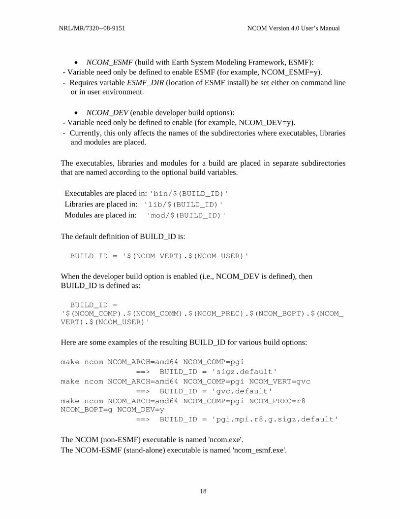
• NCOM_ESMF (build with Earth System Modeling Framework, ESMF):
- Variable need only be defined to enable ESMF (for example, NCOM_ESMF=y). - Requires variable ESMF_DIR (location of ESMF install) be set either on command line
or in user environment.
• NCOM_DEV (enable developer build options): - Variable need only be defined to enable (for example, NCOM_DEV=y). - Currently, this only affects the names of the subdirectories where executables, libraries
and modules are placed. The executables, libraries and modules for a build are placed in separate subdirectories that are named according to the optional build variables. Executables are placed in: 'bin/$(BUILD_ID)' Libraries are placed in: 'lib/$(BUILD_ID)' Modules are placed in: 'mod/$(BUILD_ID)' The default definition of BUILD_ID is: BUILD_ID = '$(NCOM_VERT).$(NCOM_USER)' When the developer build option is enabled (i.e., NCOM_DEV is defined), then BUILD_ID is defined as: BUILD_ID = '$(NCOM_COMP).$(NCOM_COMM).$(NCOM_PREC).$(NCOM_BOPT).$(NCOM_VERT).$(NCOM_USER)' Here are some examples of the resulting BUILD_ID for various build options: make ncom NCOM_ARCH=amd64 NCOM_COMP=pgi ==> BUILD_ID = 'sigz.default' make ncom NCOM_ARCH=amd64 NCOM_COMP=pgi NCOM_VERT=gvc ==> BUILD_ID = 'gvc.default' make ncom NCOM_ARCH=amd64 NCOM_COMP=pgi NCOM_PREC=r8 NCOM_BOPT=g NCOM_DEV=y ==> BUILD_ID = 'pgi.mpi.r8.g.sigz.default' The NCOM (non-ESMF) executable is named 'ncom.exe'. The NCOM-ESMF (stand-alone) executable is named 'ncom_esmf.exe'.
18

NRL/MR/7320--08-9151 NCOM Version 4.0 User’s Manual
Note: See file ncom_4.0/doc/README.make for more discussion. 4.1.3 Set Halo Width Set halo width nmh in file ncom_4.0/include/PARAM.h. Set the halo width variable nmh to 2. 4.1.4 Set Maximum Dimensions Set maximum allowed dimensions in file ncom_4.0/include/PARAM.h. These variables are used to dimension some scratch arrays in the model code. The model does not use many such scratch arrays, so the penalty in memory usage for setting these values larger than necessary is minimal. Note that some of the maximum dimensions set in PARAM.h are provided by parameters that are defined within file MACROS.h (see discussion of MACROS.h below).
nrmx - maximum allowed number of scalar fields (nr), usually =2 (T & S). nqmx - maximum allowed number of turbulence fields (nq), usually =2. nobmx - maximum allowed number of open boundary points. ntcmx - maximum allowed number of tidal constituents for tidal forcing. nrivmx - maximum allowed number of (horizontal) river inflow points. mxgrdso - maximum allowed number of ocean model grids (nests). Note: See file ncom_4.0/include/README.include for more discussion. 4.1.5 Set Macro Values Set MACRO values in file ncom_4.0/include/MACROS.h.
MXPROC - maximum number of processors (<= MX1PRC**2). MX1PRC - maximum number of processors in either direction (x or y). MN1PRC - minimum number of processors in either direction (x or y). NMXA - maximum whole array dimension in either direction (x or y). LMX - maximum vertical array dimension (max number of layers + 1). As mentioned in Section 4.1.4, setting dimensions NMXA and LMX larger than needed only incurs a small penalty in terms of memory requirements. It is recommended that all maximum dimensions be set to the largest values needed for different applications to avoid having to recompile. Other macro variables in MACROS.h are either for particular tests or applications or do not generally need to be modified by the user. See file ncom_4.0/include/README.macros for more discussion. 4.1.6 Create Executable File On the model code subdirectory (ncom_4.0) the user should type, for example,
make ncom NCOM_ARCH=ibm_sp or if a log file (Make_ncom_ibm_sp) containing a record of the compilation is needed, type:
make ncom NCOM_ARCH=ibm_sp >& Make_ncom_ibm_sp &
19

NRL/MR/7320--08-9151 NCOM Version 4.0 User’s Manual
In these examples, NCOM_ARCH defines on which machine architecture the make is running (ibm_sp, amd64, etc.). A list of the supported architecture/compiler combinations is available by listing the contents of the config directory. The architecture/compiler/user specific makefile fragments are named as $(NCOM_ARCH).$(NCOM_COMP).$(NCOM_USER).mk. The default NCOM_USER setting is “default”. See file ncom_4.0/config/README.config for information on how to create new configurations. 4.1.7 Deleting Executables and Libraries The NCOM libraries that are created are stored on ncom_4.0/lib. The NCOM executable is generated and stored on ncom_4.0/bin. To delete libraries and executables for a particular NCOM_ARCH, use:
make clean NCOM_ARCH=ibm_sp To delete all libraries and executables, use:
make clobber 4.2 Setting Up a Simulation Setting up a simulation for a new model domain or region is a multi-step process. This is also known as generating input files for a simulation. The steps are outlined below: 1. Set up a directory for a particular model simulation (call it run_sim for the purpose of
this discussion). For example, RELO_NCOM is the setup routine used in regional areas. The script ncom_prep.com is used for global and EAS NCOM runs.
2. Modify the model input parameter file OPARM_1.D on subdirectory /input for the particular simulation to be run. There is a discussion of the input parameters in file OPARM_1.D. The other files on the input subdirectory should be deleted except for the IOS_tidetbl.D, spmd.D_*, and STOP.D files.
3. Several stand alone routines exist for the purpose of creating model grid and other first-level input files for different domains. At present this process is neither a system component nor automated within the general NCOM system. However, the RELO_NCOM application of NCOM does include an automated setup for regional applications (the specifics of RELO_NCOM are discussed in separate documentation).
Note: See file run_sim/README.make for additional discussion. A note about setup programs: General setup subroutines (i.e., not specific to a particular simulation) are stored on the model directory on subdirectory libsrc/setup. The file ncom_setup_plib.F on this subdirectory contains a number of general subroutines that can be used to help set up a particular simulation. When NCOM is made, the required general libraries are compiled and put on the model subdirectory ./lib. These libraries all contain the prefix _setup.a The setup program can only be run on a single processor. Hence, all the routines used for the model setup are compiled to run on a single processor. The compilation of the setup routines uses a special configuration file on the subdirectory /config which has the suffix _setup. If such a file does not exist for the computer being
20

NRL/MR/7320--08-9151 NCOM Version 4.0 User’s Manual
used, it can be generated from the configuration file for a single processor by only making one change: the macro option -DSETUP must be added to the list of cpp compiler flags (CPPFLAGS). The –DSETUP compile option will cause the halos to be set to zero. 4.3 Running a Simulation For this discussion, the simulation directory again will be called run_sim. The simulation can be run on the original model simulation subdirectory or another one, e.g., set up on another computer or on a scratch directory. Requirements for running a simulation are (i) run script, (ii) model executable, and (iii) model input files. Some examples of run scripts are on directory /run_scripts. The run scripts for NCOM Version 4.0 include the defining of general variables, checking for existence of input files and post-processing the model output binary files into other formats for the purposes of creating graphics and statistical manipulation. A difference is that an additional input file, spmd.D_n (where n is the number of processors being used) is needed. The parameters defined in spmd.D_n are: ipr = number of processors being used in x dimension of model. jpr = number of processors being used in y dimension of model. jqr = total number of processors being used = ipr*jpr. iprsum = number of subdomains in x used for summing values over the horizontal grid. Iprsum must be a multiple of ipr, for example, iprsum = ipr * i, where i is some
integer. jprsum = number of subdomains in y used for summing values over the horizontal grid. Jprsum must be a multiple of jpr, for example jprsum = jpr*j, where j is some
integer. The simplest and most efficient setup is to set iprsum=ipr and jprsum=jpr. For example, if the user has four processors in x and three in y (i.e., 4 x 3 = 12 total), simply set iprsum=4 and jprsum=3. Alternative choices for iprsum, jprsum could be (8,3), (4,6), (8,6), (12,3), etc. The values used for iprsum, jprsum can affect the bit-for-bit reproducibility of NCOM results because the order in which an array of values is summed will affect the result, and this could affect the results of the solver used for the free surface in NCOM. Note that this only matters if we are trying to compare bit-for-bit reproducibility of model results on different numbers of processors. For example, if we want to compare results on 3x2 processors with results on 5x3 processors, we would need to use the same values of iprsum and jprsum for both runs, e.g., iprsum=15 and jprsum=6 would work. The model input files are, by default, located on directory run_sim/input, but another location can be pointed to in the run script. Similarly, the output and restart files are by default located on directories run_sim/output and run_sim/restart, but can be placed elsewhere as defined in the run script.
21

NRL/MR/7320--08-9151 NCOM Version 4.0 User’s Manual
When preparing input files or looking at output files, the subroutines in ncom1rwio.F can be used by linking in the NCOM libraries. If the user wants to employ their own code to write the input files or read the output files, this can be done by referring to ncom1rwio.F to get the proper file format. For the most part, these file formats are fairly straightforward. For example, all the *.A files are direct access (IEEE) binary with record size n*m (or n*m*4 "bytes") where n and m are the horizontal grid dimensions. The model executable is copied into the simulation directory from wherever it resides. If running on more than one processor, the executable is specific to the computer and type of communication being used. The executable is also specific to the choices made in defining parameters in the MACROS.h and PARAM.h files prior to the compile. 4.4 Model Input Files Special routines are provided to read and write 2D and 3D arrays for use in multi-processor (MP) environments with distributed memory. These parcel out input arrays to the appropriate processors and gather output from the processors into a single output file. Some specific filename extensions are used to denote the type of file: *.A - 2D and 3D array data that is parceled out to the processors. *.B - scalar data associated with the *.A file, e.g., the date and time. These files are read
in full by each processor. *.D - data files that are read in full by each processor. The *.A files are direct-access, unformatted binary files. The *.B files are formatted ASCII. The *D files may be binary or formatted ASCII. The input files also have a numerical designation to denote the model grid (nest) for the data, e.g., file OPARM_1.D is the input parameter file for grid number 1 (the main grid). The data for each grid (nest) is handled separately, so each grid or nest must have a complete set of input files and will produce its own set of output files. Note that the 2D and 3D *.A files are simply direct access, IEEE, 32-bit binary files, with the arrays written out with the same indexing sequence with which they are normally stored in memory. No compression is applied. There are different input files for different inputs. In general, if an option to use a particular type of input data (e.g., surface forcing, tides, open boundary values, or river inflow) is not used, an input file for that data will not be read and does not need to exist. If a particular input data file is not used (e.g., open boundary data, tidal data, river inflow data), the flag corresponding to that input data in the input parameter file (OPARM_n.D) may need to be set to the appropriate value (usually =0) so that the program does not try to read that data from an input file. Inputs from specific sources and for particular dates and times such as NOGAPS, MODAS, and NLOM have specific input names with date time groups and model parameter options inserted into the file names.
22

NRL/MR/7320--08-9151 NCOM Version 4.0 User’s Manual
Table 4.4-1: NCOM list and description of input files.
File Description Unit Number
IOS_tidetbl.D General tidal constituent info, e.g., tidal frequencies, node factors, phase corrections, etc.
OPARM_1.D Input parameters and options. 99+100*nest odimens.D Grid and array dimensions for all the grids (nests). 99 oextd_n.A Array data for solar extinction (chl or K490
values). 99+100*nest
oextd_n.B Scalar data for solar extinction (chl or K490 values).
ohgrd_n.A Array data for horizontal grid. 99+100*nest ohgrd_n.B Scalar data for horizontal grid. oinit_n.A Array data for initial conditions. 99+100*nest oinit_n.B Scalar data for initial conditions. opnbc_n.D Data for open boundaries. 41+100*nest orivs_n.D River inflow data. 42+100*nest osflx_n.A Array data for surface forcing fields. 31+100*nest osflx_n.B Scalar data for surface forcing fields. ossst_n.A Array data for SST and SSS relaxation. ossst_n.B Scalar data for SST and SSS relaxation. ossss_n.A Array data for SSS relaxation. ossss_n.B Scalar data for SSS relaxation. otloc_n.D List of sections for which transports are to be
output. 99+100*nest
otide_n.B List of constituents for which tidal BC data are supplied.
otide_n.D Tidal BC data (tidal constituent elevation and velocity data at the model open boundary points).
99+100*nest
otpcn_n.D List of tidal constituents for which tidal potential is calculated.
otscl_n.A Array data for T-S climatology. 99+100*nest otscl_n.B Scalar data for T-S climatology. otsf_n.A Array data to which 3D T and S fields are to be
relaxed. 35+100*nest
otsf_n.B Scalar data to which 3D T and S fields are to be relaxed.
23

NRL/MR/7320--08-9151 NCOM Version 4.0 User’s Manual
Unit File Description Number owrlx_n.A Array data for relaxation timescale (3D). 99+100*nest owrlx_n.B Scalar data for relaxation timescale. osstf_n.A Array data for which 2D SST and SSS values are to
be relaxed. 33+100*nest
osstf_n.B Scalar data for which 2D SST and SSS values are to be relaxed.
otsza_n.A Array data for horizontally averaged T and S fields. 99+100*nest otsza_n.B Scalar data for horizontally averaged T and S
fields.
outpt_n.D List of grid indices for points at which model results are output.
99+100*nest(.A)
ovgrd_n.A 3D array data for static depth to the top of each grid cell.
ovgrd_n.B Scalar data describing the vertical grid. ovgrd_n.D 1D array of static interface depths for z-level grid. 99+100*nest owmdf_n.D List of water mass definitions for which volumes
are to be calculated. 99+100*nest
ozout_n.D List of depths at which fields are to be output. 99+100*nest stop.D Stop file used to pause an interactive run to allow
inspection of model fields. 99
spmd.D_n Parameters describing the processor layout used for running on multiple processors.
99
Input files that have time-varying input such as surface forcing fields are labeled with an eight-digit integer date of the form YYYYMMDD and an eight-digit integer time of the form HHMMSSCC, where CC is hundredths of seconds. If the data in a time-varying type of input data file is provided only at a single time (i.e., is fixed in time), set the date and time integers to zero. For seasonal or monthly varying climatological data, set the year (YYYY) to zero and set the month and day according to the time of year of the field. The model will automatically cycle through time-varying input fields and interpolate the fields linearly in time to the current time of the model. Real-time input fields can cover a greater period of time than that covered by the model run, but must at least cover the time period of the model run. Climatological fields will automatically be cycled around at the end of the year. Input data specified only at a single time (with date and time set to zero) will remain fixed during the run.
24

NRL/MR/7320--08-9151 NCOM Version 4.0 User’s Manual
4.5 Model Output Files Some model output data files are provided, such as surface and 3D fields. The model output files are written from subroutine OUTPUT. The user may wish to modify the model output for his/her own needs. The model subroutines in file ncom1rwio.F for reading/writing output files can be modified, or the fields can be output in a format preferred by the user. For MP use, array data from the different processors must be gathered, so the user may wish to modify the corresponding output subroutines in ncom1rwio.F rather than write their own routine from scratch. Output files currently provided are:
Table 4.5-1: Output Files
File Description Unit Number
out3d_n.A Array data for 3D output fields. 51+100*nest out3d_n.B Scalar data for 3D output fields. 51+100*nest outsf_n.A Array data for 2D surface output fields. 52+100*nest outsf_n.B Scalar data for 2D surface output fields. 52+100*nest knrgy_n.D Volume averaged kinetic energy. 56+100*nest otran_n.D Transport through specified sections. 57+100*nest pt_nn.D Profiles of model fields at a specified point (pt
number nn). 61-98+100*nest
Post-processing programs can use the subroutines in ncom1rwio.F to read the output files by linking ncom1rwio.o and a couple of support libraries. See file ncom_images.u for an example. The time that is included with the output fields is the elapsed time in days since the start of the model run. This can be combined with the model start time (in OPARM_1.D) to obtain the actual time and date of the fields. 4.6 Input Parameters in File OPARM_1.D. The parameters in file OPARM_1.D provide some control over a number of aspects of the ocean model run, including the model physics and numerics, the forcing, and the output. modelo- name of model (NCOM1) being used. expto- name of experiment. domain- name of domain.
25
NRL/MR/7320--08-9151 NCOM Version 4.0 User’s Manual
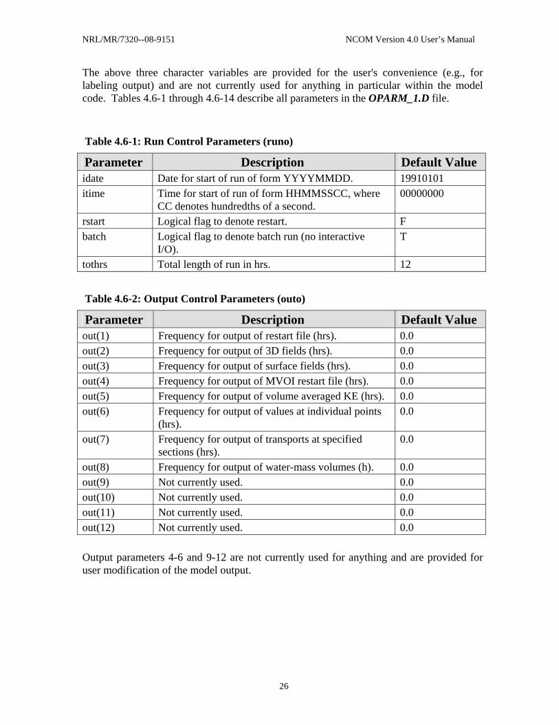
The above three character variables are provided for the user's convenience (e.g., for labeling output) and are not currently used for anything in particular within the model code. Tables 4.6-1 through 4.6-14 describe all parameters in the OPARM_1.D file.
Table 4.6-1: Run Control Parameters (runo)
Parameter Description Default Value idate Date for start of run of form YYYYMMDD. 19910101 itime Time for start of run of form HHMMSSCC, where
CC denotes hundredths of a second. 00000000
rstart Logical flag to denote restart. F batch Logical flag to denote batch run (no interactive
I/O). T
tothrs Total length of run in hrs. 12
Table 4.6-2: Output Control Parameters (outo)
Parameter Description Default Value out(1) Frequency for output of restart file (hrs). 0.0 out(2) Frequency for output of 3D fields (hrs). 0.0 out(3) Frequency for output of surface fields (hrs). 0.0 out(4) Frequency for output of MVOI restart file (hrs). 0.0 out(5) Frequency for output of volume averaged KE (hrs). 0.0 out(6) Frequency for output of values at individual points
(hrs). 0.0
out(7) Frequency for output of transports at specified sections (hrs).
0.0
out(8) Frequency for output of water-mass volumes (h). 0.0 out(9) Not currently used. 0.0 out(10) Not currently used. 0.0 out(11) Not currently used. 0.0 out(12) Not currently used. 0.0 Output parameters 4-6 and 9-12 are not currently used for anything and are provided for user modification of the model output.
26

NRL/MR/7320--08-9151 NCOM Version 4.0 User’s Manual
Table 4.6-3: Output Control Parameters for Surface Fields (iouto)
Parameter Description Default Value inde2 Include surface elevation: 0= no, =1 yes. 1 indvb2 Include barotropic transport: =0 no, =1 yes. 1 indv2 Include surface velocity: =0 no, =1 yes. 1 indt2 Include surface temperature: =0 no, =1 yes. 1 inds2 Include surface salinity: =0 no, =1 yes. 1 inda2 Include surface windstress: =0 no, =1 yes. 1
Table 4.6-4: Output Control Parameters for 3D Fields Output File (iouto)
Parameter Description Default Value inde3 Include surface elevation: =0 no, =1 yes. 1 indvb3 Include barotropic transport: =0 no, =1 yes. 1 indv3 Include 3D u and v velocity: =0 no, =1 yes. 1 indw3 Include 3D vertical velocity: =0 no, =1 yes. 0 indt3 Include 3D temperature: =0 no, =1 yes. 1 inds3 Include 3D salinity: =0 no, =1 yes. 1 inda3 Include surface atmospheric forcing: =0 no, =1
yes. 1
idatnow Date for nowcast, end hindcast, start forecast (YYYYMMDD).
99990101
itimnow Time for nowcast, end hindcast, start forecast (HHMMSSCC).
0
irs_out Output NFS restart file: =1 once; =2 at reg intervals.
1
irs_date NFS restart file data type: =0 none; =1 date_time; =2 date-time group (YYYYMMDDHH).
0
irs_mean Save values in array rmean to restart file: =0 no; =1 yes.
0
irs_fmt Restart *.B file being read: =0 unformatted with elapsed time of restart fields (old-style); =1 formatted with date-time of restart fields (new-style).
1
irs_rset Reset elapsed time and iteration count to zero when reading old-style unformatted restart *.B file; =0 no; =1 yes. This has no effect if reading new-style formatted restart *.B file.
0
ioutdate Type of date-time tag to use for surface and 3D output files.
0
ioutnow Write surface and 3D output files:: = -1 only before 0
27

NRL/MR/7320--08-9151 NCOM Version 4.0 User’s Manual
Parameter Description Default Value the nowcast time; =0 at all times; =1 only after the nowcast time.
irlx2now Relax SST and SSS: =0 no, =1 yes. 0 irlx3now Relax 3D T and S: =0 no, =1 yes. 0
Table 4.6-5: Physical Options (phyo)
Parameter Description Default Value mode Mode: =1 1D ML; =2 2D barotropic; =3 full 3D; =4
diagnostic. 3
indcor Coriolis flag: =0 none; =1 constant, =2 variable. 2 indden Density calculation: =1 Frederich-Levitus (1972).
This is fast and derived for seawater, so accuracy may be low in fresh water; =3 UNESCO formula (Mellor, 1991) has good accuracy but is expensive (50+ operations per point) and adds about 18% to the model run time.
3
indadv Momentum advection: =0 off; =1 on. 1 indadvr Scalar advection: =0 off; =1 on; =2 FCT adv. 1 indxk Horizontal diffusion: =0 none; =1 Laplacian mixing
grid-cell-Re mixing with grid-cell-Re=xkre. Minimum mixing coefficients in x and y are set by xkmin and ykmin, respectively; =2 Laplacian Smagorinsky mixing scaled by parameter smag. Note: The use of Smagorinsky with smag=0.1 tends to give results similar to the grid-cell-Re scheme with a value of xkre of ~ 15-20.
2
indzk Vertical mixing: =1 constant (values set by zkmmin and zkhmin below); =2 MYL2; =4 MYL2.5 with option for Craig and Banner (1994) treatment of surface TKE flux and length scale (see parameter indtkes below).
2
indtkes Treatment of TKE BC for indzk=4: =1 surface value of TKE (scaled as [surface friction velocity]2); =2 surface TKE flux (scaled as [surface friction velocity]3).
2
indlxts Relax deep T and S to climatology: =0 no; =1 relax to T and S climate fields in array rmean; =2 relax to time-varying input T and S fields.
0
indext Solar extinction: =0 none; =1 Jerlov optical types. Note: The solar extinction within NCOM is stored
1
28

NRL/MR/7320--08-9151 NCOM Version 4.0 User’s Manual
Parameter Description Default Value in a 3D array (ext) so that full spatial and temporal variability can be accommodated. I/O for such variability is not currently provided, but can be set up by the user. All solar radiation penetrating the upper surface of the bottom layer is absorbed within the bottom layer.
indtype Seawater Jerlov optical type (if constant type is used). =1 type I; =2 type IA; =3 type IB; =4 type II; =5 type III.
2
indbio Biological model: =0 none; =1 4-component. 0 indice Ice model: =0 none; =1 SST limited to >= -0.54C. 0 bclinic Baroclinic pressure gradients calculated. T curved Horizontal advection grid curvature term
calculated. This should be set to "true" when a curvilinear grid (i.e., a non-Cartesian grid such as a longitude-latitude grid) is used and can be set "false" when a Cartesian (non-curved) grid is used.
T
noslip No slip lateral BC for momentum at land-sea boundaries. =0 use free slip; =1 use no-slip.
T
sigdif Logical flag to subtract climate values (stored in array rmean) from scalar fields when performing horizontal diffusion along sigma layers. This prevents much of the effective vertical diffusion of scalar fields that can occur along sloping sigma layers, though it can cause other problems when the local values of the scalar field differ from the climate values provided. Generally, however, the latter problem is less than the former problem and sigdif is usually set = .true. These problems are reduced as grid resolution is increased and horizontal mixing is reduced and/or bottom slopes are reduced. For third-order upwind advection (UPW3), when sigdif = true, the climate value is subtracted off the T and S values used to calculate the fourth-order correction to the advection flux and the biharmonic mixing flux at the grid cell boundary. As with the diffusion term, there is potential for problems with the use of this procedure.
T
largmix Use Large et al. (1994) Richardson-number-dependent background mixing for Richardson numbers above critical but less than 0.7. Currently this is only implemented when using Mellor-
T
29

NRL/MR/7320--08-9151 NCOM Version 4.0 User’s Manual
Parameter Description Default Value Yamada Level 2 mixing (indzk=2).
Table 4.6-6: Physical parameters (phyp)
Parameter Description Default Value
rho0 Reference density for seawater (kg/m3). 1025.0 g Gravitational constant (m/s2). 9.8 cp Specific heat for seawater (Joules/kg/°C). 3994.0 ramphrs Length of ramp function for ramping baroclinic
pressure gradients, surface forcing, boundary forcing, etc. (hrs).
0.0
xkmin Minimum horizontal momentum mixing coefficient in x for grid-cell Reynolds number mixing scheme (m2/s), and also a minimum horizontal mixing coefficient for the Smagorinsky scheme.
0.0
ykmin Minimum horizontal momentum mixing coeff. in y for grid-cell Reynolds number mixing scheme (m2/s), usually set the same as xkmin.
0.0
xkre Maximum horizontal grid-cell Reynolds number for grid-cell Reynolds number mixing scheme.
100.0
smag Scaling constant for Smagorinsky horizontal mixing scheme (same as parameter "horcon" in POM).
0.1
prnxi Inverse Prandtl number for horizontal mixing. A value smaller (larger) than 1.0 will reduce (increase) the mixing for scalar fields proportionally.
1.0
zkmmin Minimum vertical diffusion coefficients for momentum (m2/s).
0.1e-4
zkhmin Minimum vertical diffusion coefficients for scalar fields (m2/s).
0.1e-4
zkre Maximum vertical grid-cell Reynolds number (only used with MYL2 mixing, i.e., with indzk=2).
2000.0
cbmin Minimum value for bottom drag coefficient. 0.0025 botruf1 Bottom roughness (m) if constant value is used.
This is used to calculate the bottom drag coefficient and assumes a logarithmic bottom boundary layer.
0.010
rlax_ts Timescale for relaxation of deep T and S fields to specified values (hrs). If rlax_ts=0, a 3D timescale field (stored in files owrlx_*.A and owrlx_*.B) is read in and used. With this 3D timescale field, the timescale can be separately specified at each model
6000.0
30

NRL/MR/7320--08-9151 NCOM Version 4.0 User’s Manual
Parameter Description Default Value
grid pt. This allows stronger relaxation in specified areas, e.g., near open boundaries.
rlax_ds Depth scale for relaxation of deep T and S fields to specified values (see indlxts above) in hrs.
500.0
b1_my12 Mellor Yamada Level 2 dissipation constant. Larger values decrease dissipation and increase vertical mixing.
15.0
Table 4.6-7: Numerical options (numo)
Parameter Description Default Value
itermom Number of iterations of baroclinic momentum equations.
1
indbaro Method of solution used for free surface mode: =1 full explicit, the model is run with a single (very small) explicit timestep; =2 semi-implicit; =3 split-explicit (not implemented).
2
indsolv Solver used to calculate the semi-implicit free surface: =1 solvel; =2 sorcyc2 (non-sym); =3 sorcyc2 (symmetric solver).
1
indrag Bottom drag calculation used only when model is run with a single layer (i.e., with l=ls=2); =1 explicit bottom drag; =2 pseudo implicit; =3 fully implicit (best choice).
2
ifdadrh Horizontal adv. of scalars: =2 second-order; =3 UPW3 (quasi third-order upwind). When UPW3 horizontal advection is used, bi-harmonic mixing is implicitly included and Laplacian horizontal mixing is not used.
2
ifdadrv Vertical advection of scalars: =2 second-order; =3 UPW3. When FCT advection is used (indadvr=2), the high-order advection scheme for the scalar fields is set by ifdadrh and ifdadrv, i.e., when these are set =2, second-order advection is used; = 3 UPW3 is used; = 4, fourth-order advection is used.
2
ifdaduh Horizontal advection of momentum: =2 second-order; =3 UPW3. When UPW3 horizontal advection is used, bi-harmonic mixing is included and
2
31

NRL/MR/7320--08-9151 NCOM Version 4.0 User’s Manual
Parameter Description Default Value
Laplacian horizontal mixing is not used. ifdaduv Vertical advection of momentum: =2 second-order;
=3 UPW3. 2
ifdpgrd Horizontal baroclinic pressure gradient: =2 second-order; =4 fourth-order.
2
ifdcor Horizontal interpolation of Coriolis terms: =2 second-order; =4 fourth order.
2
forward Use forward scheme on first timestep of a cold start (this is the usual choice - use of leapfrog on first timestep would require a special initialization of the model fields at the previous time level). For now, always set forward = true. Note that for restarts, fields at two adjacent timesteps are stored in the restart file, and restarts automatically always use a leapfrog first timestep.
T
vector Use vectorizable subroutines. Always set vector = true.
T
shrnkwp Use shrinkwrapping. Shrinkwrapping can save considerable time on a single processor, depending on the configuration of the domain. Do not use when running on multiple processors. Note that results with and without shrinkwrapping should be identical and it is recommended that the user check for this on their particular model setup.
F
Table 4.6-8: Numerical parameters (rnumo)
Parameter Description Default Value
dti Internal model timestep(s). The maximum timestep is governed by the maximum advective and internal wave speeds. For numerical stability, a parcel of fluid cannot be advected or a wave cannot propagate more than one grid distance in one "leapfrog timestep" (= 2*dti). A rough estimate for an allowable timestep is to take the horizontal grid spacing in km and multiply by 120, e.g., for a 1 km grid, use dti=120s. This timestep should be stable for most internal wave and horizontal advective speeds encountered in the ocean. However, with high vertical resolution and thin vertical layers, vertical advection may limit the timestep. The advective CFL values (2*dti*velocity/grid_spacing) are printed
180.0
32

NRL/MR/7320--08-9151 NCOM Version 4.0 User’s Manual
periodically by the model to allow them to be monitored. dte External timestep (s) for split-explicit scheme (not
used). 5.0
asf Asselin filter coefficient for temporal filtering to prevent timesplitting with the leapfrog temporal integration scheme.
0.05
eg1 Temporal weight for implicit surface elevation at new time.
0.50
eg2 Temporal weight for implicit surface elevation at previous timestep.
0.00
vg1 Temporal weight for momentum in continuity eqn at new time.
0.50
vg2 Temporal weight for momentum in continuity eqn at previous timestep.
0.00
cb_filt Checkerboard mixing filter value (-0.125 to 0.125). Set this value positive for 5-pt filter and negative for 9-pt filter, e.g., = -0.125 max 9-pt filter; = 0 no filter; = 0.125 max 5-pt filter. The 9-pt filter gives the strongest filtering.
0.0
cb_dep Depth of application of checkerboard filter (+m). Strength of filtering is decreased linearly from max at surface to zero at this depth.
50.0
Table 4.6-9: Surface Forcing Options And Parameters (isbco, lsbco, sbco)
Parameter Description Default Value
indsbc Atmospheric forcing: =0 none (all atm forcing is turned off); =1 turned on according to parameters below.
0
indatp Surface atmospheric pressure forcing; =0 none; =1 from input data file; =2 from coupled atm model; =3 directly from COAMPS atm model flat file output interpolated spatially to NCOM ocean grid.
0
indtau Surface wind stress forcing. =0 none; =1 data file; =2 coupled atm model; =3 COAMPS flat file output.
0
indsft Surface heat flux: =0 none; =1 data file; =2 coupled atm model; =3 COAMPS flat file output; =4 same as 3 but use bulk formulas with COAMPS (flat file) air temperature and humidity and NCOM-predicted SST to compute latent and sensible heat fluxes; =5 same as 1 but use bulk formulas and air temperature and humidity (from input file) and NCOM SST to compute latent and sensible heat fluxes.
0
33
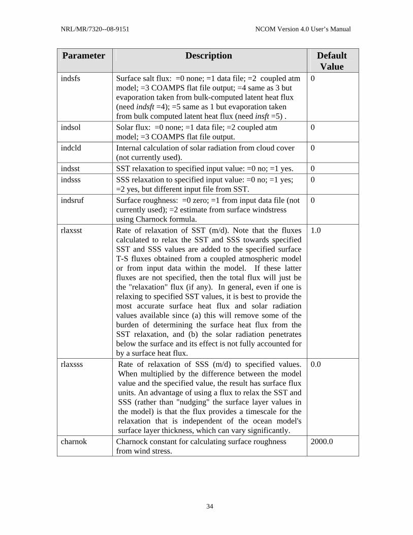
NRL/MR/7320--08-9151 NCOM Version 4.0 User’s Manual
Parameter Description Default Value
indsfs Surface salt flux: =0 none; =1 data file; =2 coupled atm model; =3 COAMPS flat file output; =4 same as 3 but evaporation taken from bulk-computed latent heat flux (need indsft =4); =5 same as 1 but evaporation taken from bulk computed latent heat flux (need insft =5) .
0
indsol Solar flux: =0 none; =1 data file; =2 coupled atm model; =3 COAMPS flat file output.
0
indcld Internal calculation of solar radiation from cloud cover (not currently used).
0
indsst SST relaxation to specified input value: =0 no; =1 yes. 0 indsss SSS relaxation to specified input value: =0 no; =1 yes;
=2 yes, but different input file from SST. 0
indsruf Surface roughness: =0 zero; =1 from input data file (not currently used); =2 estimate from surface windstress using Charnock formula.
0
rlaxsst Rate of relaxation of SST (m/d). Note that the fluxes calculated to relax the SST and SSS towards specified SST and SSS values are added to the specified surface T-S fluxes obtained from a coupled atmospheric model or from input data within the model. If these latter fluxes are not specified, then the total flux will just be the "relaxation" flux (if any). In general, even if one is relaxing to specified SST values, it is best to provide the most accurate surface heat flux and solar radiation values available since (a) this will remove some of the burden of determining the surface heat flux from the SST relaxation, and (b) the solar radiation penetrates below the surface and its effect is not fully accounted for by a surface heat flux.
1.0
rlaxsss Rate of relaxation of SSS (m/d) to specified values. When multiplied by the difference between the model value and the specified value, the result has surface flux units. An advantage of using a flux to relax the SST and SSS (rather than "nudging" the surface layer values in the model) is that the flux provides a timescale for the relaxation that is independent of the ocean model's surface layer thickness, which can vary significantly.
0.0
charnok Charnock constant for calculating surface roughness from wind stress.
2000.0
34

NRL/MR/7320--08-9151 NCOM Version 4.0 User’s Manual
Lateral boundary options: There are a number of options for open BC provided here that have been implemented for various reasons, such as for testing or special cases. The generally recommended BCs are:
1. For the free surface: indobe=2 (Flather). 2. For tangential velocities: indobvb=indobv=1 (zero gradient normal to the
boundary, though the Orlanski BC (indobvb=indobv=2) is also good. 3. For the normal baroclinic velocity: indobu=3 (model internally calculated value
plus upstream advection normal to the boundary). 4. For scalar fields: indobr=2 (Orlanski). 5. For nesting with feedback: indobr=1 (put the externally provided value directly on
the boundary). In these descriptions of the BC, the "external" value refers to an externally provided value from a larger-scale model simulation, climatology, data, etc.
Table 4.6-10: Lateral Boundary Options (iobco)
Parameter Description Default Value
indcyc Flag to denote periodic cyclic bndys: =0 none; =4 x; =5 y; =6 x & y. Periodic boundaries are very useful for test problems and also allow the model to be run in pseudo 2D and pseudo 1D mode. Periodic boundaries used to be implemented using a 3-pt overlap (with indcyc=1-3), however, they are now implemented using the halos around the edge of the model grid.
0
indtide Includes specified tidal forcing at open boundaries. It requires an input file of tidal data for the open boundary points, consisting of the amplitude and phases of the surface elevation and normal and tangential velocities. Ask Paul Martin about implementing tidal forcing.
0
indobc =0 no open bndys; =1 use IC; =2 use input file; =3 interpolate from the parent grid for a nested grid.
1
indobe Open boundary conditions for surface elevation; =1 clamped. This is generally used only when tidal forcing is used at the boundary. In this case, only tidal elevation data are needed at the boundary, not tidal velocity; =2 Flather. This is the primary open boundary condition used since it handles radiation of barotropic disturbances out of the model domain. When this BC is used, both the elevation and normal velocity (the depth-
2
35

NRL/MR/7320--08-9151 NCOM Version 4.0 User’s Manual
Parameter Description Default Value
averaged normal velocity times the local depth) data at the boundary are needed.
indobvb Open boundary condition for depth-averaged tangential velocity: =1 zero gradient, i.e., set the same as interior value; =2 Orlanski radiation for outward propagating signals,
and relax to externally specified value (depth-averaged tangential velocity times depth) for incoming signals;
=3 advective boundary.
1
indobu Open boundary condition for normal baroclinic velocity: =1 calculated internally by the model. This calculation
includes all the momentum terms except advection and horizontal mixing;
=2 Orlanski radiation for outgoing signals and relax to externally specified value for incoming signals;
=3 model calculated value as in (1) plus upwind horizontal advection using the interior values to calculate the advection for outflow and external (specified) values to calculate advection for outflow. This may be the best BC for the normal velocity;
=4 advective boundary condition.
3
indobv Open boundary condition for tangential baroclinic velocity: =1 zero gradient, i.e., set same as interior value; =2 Orlanski radiation for outgoing signals and relax to
externally specified value for incoming signals; =3 advective boundary condition.
1
indobr Open boundary condition for scalar fields (T and S): =1 set directly from specified value (used with two-way
nesting when there is feedback of the T and S fields to the larger grid);
=2 Orlanski radiation for outgoing signals and relax to externally specified value for incoming signals (generally the best BC for scalars);
=3 advective boundary condition (not generally a good choice);
=4 advective boundary condition; =5 2D radiation condition.
2
36
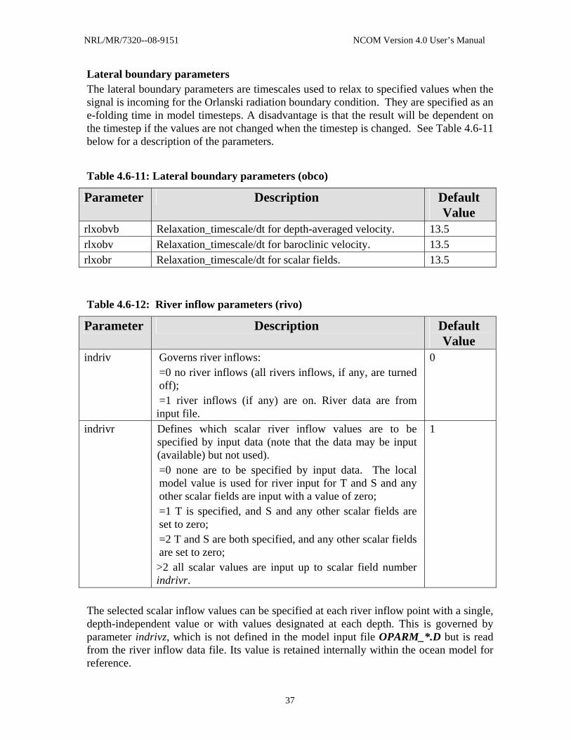
NRL/MR/7320--08-9151 NCOM Version 4.0 User’s Manual
Lateral boundary parameters The lateral boundary parameters are timescales used to relax to specified values when the signal is incoming for the Orlanski radiation boundary condition. They are specified as an e-folding time in model timesteps. A disadvantage is that the result will be dependent on the timestep if the values are not changed when the timestep is changed. See Table 4.6-11 below for a description of the parameters.
Table 4.6-11: Lateral boundary parameters (obco)
Parameter Description Default Value
rlxobvb Relaxation_timescale/dt for depth-averaged velocity. 13.5 rlxobv Relaxation_timescale/dt for baroclinic velocity. 13.5 rlxobr Relaxation_timescale/dt for scalar fields. 13.5
Table 4.6-12: River inflow parameters (rivo)
Parameter Description Default Value
indriv Governs river inflows: =0 no river inflows (all rivers inflows, if any, are turned off); =1 river inflows (if any) are on. River data are from input file.
0
indrivr Defines which scalar river inflow values are to be specified by input data (note that the data may be input (available) but not used). =0 none are to be specified by input data. The local model value is used for river input for T and S and any other scalar fields are input with a value of zero; =1 T is specified, and S and any other scalar fields are set to zero; =2 T and S are both specified, and any other scalar fields are set to zero; >2 all scalar values are input up to scalar field number indrivr.
1
The selected scalar inflow values can be specified at each river inflow point with a single, depth-independent value or with values designated at each depth. This is governed by parameter indrivz, which is not defined in the model input file OPARM_*.D but is read from the river inflow data file. Its value is retained internally within the ocean model for reference.
37

NRL/MR/7320--08-9151 NCOM Version 4.0 User’s Manual
Note: The river inflow points must be ordered (sorted) with respect to their horizontal (i,j) location. Specifically, they must be ordered in the same way that a 2D (i,j) array is stored in memory. Hence, river point (3,5) should come before river point (3,20) and river point (5,2) should come before river point (3,4). This ordering makes the handling of the river data more efficient within the model (Barron and Smedstad, 2002).
Table 4.6-13: Grid Nesting Parameters (nsto)
Parameter Description Default Value
nst (1) Grid number (each grid or nest is given an integer value, starting with "1" for the main grid).
1
nst (2) Grid number of grid in which nested (parent grid). 0 nst (3) Grid nesting ratio, must be integer value. 0 nst (4) Timestep ratio, must be integer value. . 0 nst (5) i-index of lower-left corner of grid in which nested. 0 nst (6) j-index of lower-left corner of grid in which nested. 0 nst (7) Integer flag to denote feedback of T and S fields from the
nested grid to the parent grid: =0 no feedback; =1 replace T and S on parent grid with averaged values
from the nested grid.
0
Table 4.6-14: Diagnostics Parameters (diago)
Parameter Description Default Value
indiag Level of diagnostic printouts: =0 no diagnostics printed; =1 print just the number of iterations of the implicit free surface solver.
1
locate Print out names of subroutines entered. F Note: The model input parameters are read by subroutine DEFINE in file ncom1init.F.
4.7 Parameters in File PARAM.h
Table 4.7-1: Parameters listed in PARAM.h.
Parameter Description nmh Halo width. The requirements for setting this variable are discussed in
Section 4.1.3. Halos are needed for communication when running on
38

NRL/MR/7320--08-9151 NCOM Version 4.0 User’s Manual
Parameter Description multiple processors and when using periodic boundary conditions. They are also needed when using fourth-order finite differences because mask values are required and array values accessed at the halo locations (even though the array values are masked to zero). The value of nmh must be set to 2.
nmxa Maximum allowed horizontal grid dimension. nmx Maximum allowed horizontal grid dimension on a single processor. lmx Maximum allowed vertical grid dimension (l). nrmx Maximum allowed number of scalar fields (nr). nqmx Maximum allowed number of turbulence fields (nq). nobmx Maximum allowed number of open boundary points (nob). ntcmx Maximum allowed number of tidal constituents (ntc). nrivmx Maximum allowed number of river inflow points (nriv). mxgrdso Maximum allowed number of ocean model grids (nests). The maximum allowed array dimensions listed above are used to allocate space for scratch arrays. The scratch array space dimensioned by these parameters is relatively small. Most of the scratch arrays needed by NCOM have dynamically allocated memory space "up front" and are passed through the subroutine argument lists to subroutines where they are needed. Therefore, fairly large maximum values can be allotted to the PARAM.h parameters without adding much to the memory requirements of the model. The other parameters in this file should not need to be changed. Note that nmxa, nmx, and lmx are now set by variables defined in file MACROS.h, i.e.,: nmxa=NMXA nmx =nmxa/MN1PRC lmx =LMX, where NMXA, MN1PRC, and LMX are defined in MACROS.h. 4.8 Parameters in file MACROS.h MACROS.h contains parameters for customizing the compilation of NCOM. The NCOM code is run through a preprocessor before being compiled and macros defined in MACROS.h can be used to set certain options that modify the compiled code. The user-defined macros in MACROS.h are described in Table 4.8-1:
Table 4.8-1: User-defined macros of MACROS.h.
Parameter Description MXPROC Maximum number of processors (<= MX1PRC**2). MX1PRC Maximum number of processors in either direction.
39

NRL/MR/7320--08-9151 NCOM Version 4.0 User’s Manual
Parameter Description MN1PRC Minimum number of processors in either direction. NMXA Maximum whole (total) array dimension in either direction. LMX Maximum vertical array dimension. ARCTIC Used for a global domain, where a special “arctic overlap” is used
for halo exchanges along the northern boundary. GLOBAL Implements special code for running global domain. MYL2P5 Allows for running Mellor-Yamada Level 2.5 mixing. COAMPS Implements code for running in COAMPS environment, e.g.,
using COAMPS flat files for atmospheric forcing. SYM4 Provides check for 4-fold symmetry in domain, used for testing
only. SYM8 Provides check for 8-fold symmetry in domain, used for testing
only. Other macros defined in MACROS.h are not normally modified. See "README.macros" for more info. 4.9 COAMPS Namelist Parameters Files These parameters govern the use of atmospheric forcing from files previously directly output by the COAMPS atmospheric model. The atmospheric forcing in this case is computed by NCOM during the ocean model run (i.e., rather than being preprocessed before the run) by reading in the atmospheric fields, interpolating the fields from the atmospheric model grid to the ocean grid, and then computing the needed air-sea fluxes. Output from other atmospheric models can be used in this way if the output fields are formatted (or reformatted) like COAMPS-style flat files.
Table 4.9-1: COAMPS Namelist Parameters (omnl.h)
Parameter Type Description Default Value cstlne Real 0 dbcrit Real 0 dmax Real Maximum depth. 4000. dmin Real Minimum depth. 10. dtf Real Time step for COAMPS surface
forcing (s). MAX_GRIDS*3600
dtt Real Time step for COAMPS SST (s). 43200. dtcyc Real Length of COAMPS analysis/forecast
cycle (s). 43200.
dtmin Real Minimum forecast time for using COAMPS fields (s).
3600.
40
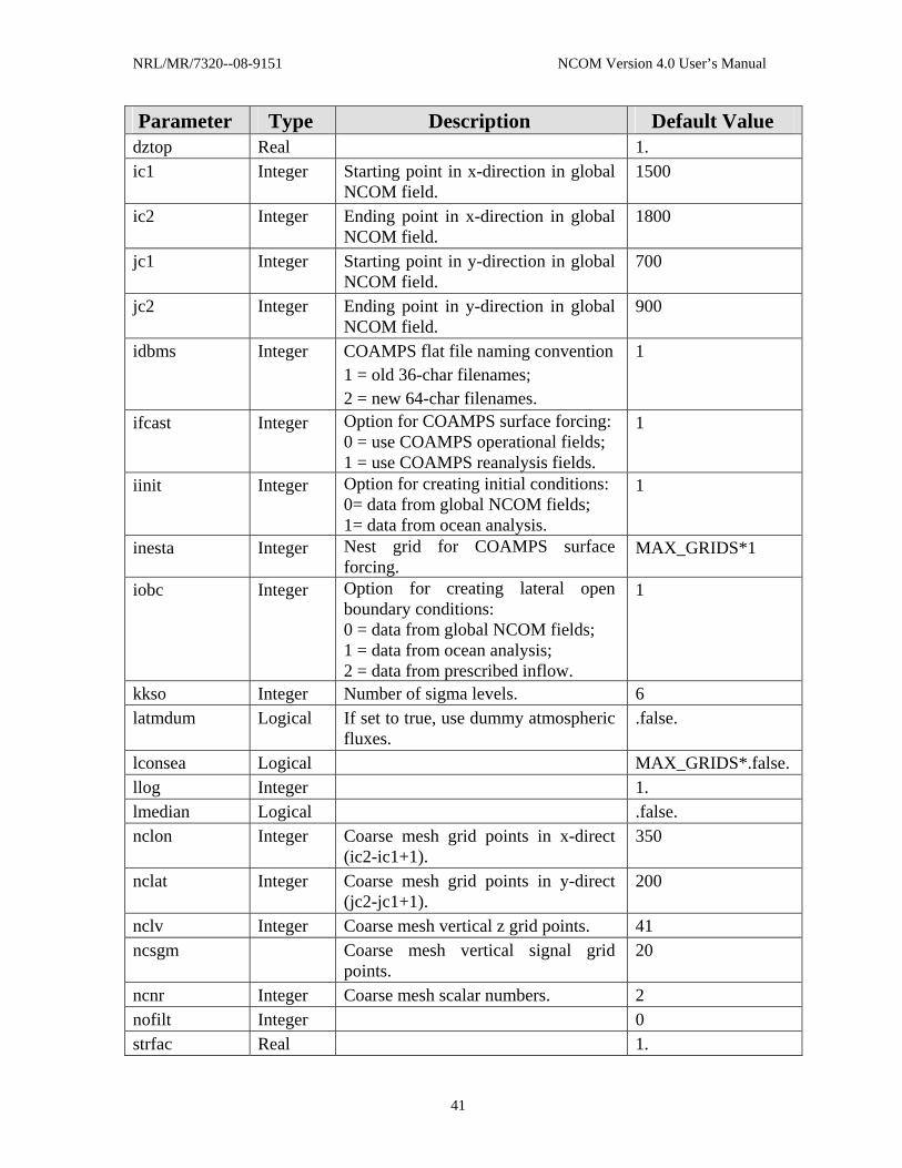
NRL/MR/7320--08-9151 NCOM Version 4.0 User’s Manual
Parameter Type Description Default Value dztop Real 1. ic1 Integer Starting point in x-direction in global
NCOM field. 1500
ic2 Integer Ending point in x-direction in global NCOM field.
1800
jc1 Integer Starting point in y-direction in global NCOM field.
700
jc2 Integer Ending point in y-direction in global NCOM field.
900
idbms Integer COAMPS flat file naming convention 1 = old 36-char filenames; 2 = new 64-char filenames.
1
ifcast Integer Option for COAMPS surface forcing: 0 = use COAMPS operational fields; 1 = use COAMPS reanalysis fields.
1
iinit Integer Option for creating initial conditions: 0= data from global NCOM fields; 1= data from ocean analysis.
1
inesta Integer Nest grid for COAMPS surface forcing.
MAX_GRIDS*1
iobc Integer Option for creating lateral open boundary conditions: 0 = data from global NCOM fields; 1 = data from ocean analysis; 2 = data from prescribed inflow.
1
kkso Integer Number of sigma levels. 6 latmdum Logical If set to true, use dummy atmospheric
fluxes. .false.
lconsea Logical MAX_GRIDS*.false. llog Integer 1. lmedian Logical .false. nclon Integer Coarse mesh grid points in x-direct
(ic2-ic1+1). 350
nclat Integer Coarse mesh grid points in y-direct (jc2-jc1+1).
200
nclv Integer Coarse mesh vertical z grid points. 41 ncsgm Coarse mesh vertical signal grid
points. 20
ncnr Integer Coarse mesh scalar numbers. 2 nofilt Integer 0 strfac Real 1.
41

NRL/MR/7320--08-9151 NCOM Version 4.0 User’s Manual
The parameters in Table 4.9-2 below govern the output of NCOM fields formatted like COAMPS-style flat files. These "flat" files are direct-access, binary files that contain one field per time per file. The fields are output on the model grid for a single vertical layer, or on the full 3D model grid (i.e., at all the model layers). They may also be output at a single depth or a number of fixed depths. The particular field, the grid dimensions, and the date-time of the field are coded into the filename. An associated, COAMPS-style "data record" file can be generated that contains additional information about the grid.
Table 4.9-2: COAMPS OMNLOFF Parameters (omnloff.h)
Parameter Type Default Value outff Logical .false. out_dir Character ‘output’ idbms_o Integer 1 offpa Real 0.0 offtx Real 0.0 offqr Real 0.0 offq0 Real 0.0 offep Real 0.0 offse Real 0.0 offsv Real 0.0 offst Real 0.0 offss Real 0.0 offmv Real 0.0 offmt Real 0.0 offms Real 0.0 offzv Real 0.0 offzt Real 0.0 offzs Real 0.0
Table 4.9-3: COAMPS Atmospheric and Ocean Parameters (dsetnl.h)
Parameter Type Description Atmospheric dsclim Character Climatology data used to initialize surface parameters
(albedo, SST, grdwet, rland, zsfc, z0) when high resolution data is not available.
dsdted Character
1 km terrain data used for horizontal resolution < 20 km.
dsgiss Characte Goddard Institute Space Studies high resolution albedo
42

NRL/MR/7320--08-9151 NCOM Version 4.0 User’s Manual
Parameter Type Description r and z0 data.
dsgoes Character
GOES real coefficients database.
dsland Character
Land sea database.
dslanu Character
Land use database.
dset1d Character
Coarse 1D graphics output directory.
dsngff Character
NOGAPS flat files used for boundary conditions and/or cold start initial conditions.
Ocean dsoclim Characte
r Ocean climate file directory path.
dsomdas Character
MODAS database file directory path.
dsorff Character
Ocean restart file directory path.
dsoudat Character
Ocean unclassified data directory.
dsordat Character
Ocean restricted data directory.
dsocdat Character
Ocean confidential data directory.
dsosdat Character
Ocean secret data directory.
Table 4.9-4: COAMPS Parameters (coamps_parms.h)
Parameter Type Description Default Value
MAX_GRIDS Integer Maximum number of grid nests. 7 MAX_NLVLS Integer Maximum number of grid nest levels. 7 MAX_IT Integer Maximum number of time iterations. 5000 4.10 Interactive Printing and Plotting Both RELO_NCOM and ncom1 are set up to do interactive printing and plotting of fields on NRL-SSC's Sun workstations. On other computers, the required plotting routines may not be available, though fields may still be printed for inspection. NCAR graphics routines are used for plotting. With minimal effort, NCAR graphics available on other computers
43

NRL/MR/7320--08-9151 NCOM Version 4.0 User’s Manual
most likely could be made to work. With a bit more effort other graphics software could be substituted for the NCAR graphics calls. The linking of the plotting software is handled by the environmental variable plotfiles that is set in the computer configuration files on subdirectory /config. In the configuration file for the NRL-SSC Sun Ultra 2 Workstations (sun_one), plotfiles is set to several files used to do NCAR plotting. In the configuration files for other computers, plotfiles is set to ../../lib/libpdum_$(TYPE).a to link in some "dummy" plotting routines that are in file libsrc/ncom/libpdum.F. These routines allow for printing out model fields, but not plotting. 4.11 Doing a Model Restart When the restart parameter is set to T (true) the model will look for a restart file. Restarts should be seamless, i.e., results after a restart should be bit-for-bit identical to results obtained without a restart. Because of the leapfrog time-stepping scheme used by the model, the restart uses model fields saved in the restart file at two successive timesteps. Previous versions of NCOM disallowed changing the model timestep on a restart. One reason was that the model elapsed time, which is computed as (number of iterations since start of run)*(timestep), would be incorrect. This restriction has been lifted by including a recalculation of the number of iterations ("iter") just after the call to read the restart file in subroutine OMODEL. The variable iter is redefined according to the new timestep as iter = times/dti. Note, however, that changing the timestep will apply a slight "jolt" to the model when it restarts because the two time levels of fields that are saved for the restart are separated by a different timestep than the one now being used. If the change in the timestep is fairly small, the jolt to the model should be minimal and the solution should, in time, adjust to the new timestep. Obviously, if the timestep is changed the restart will not be seamless.
4.12 Checking For Bit-For-Bit Reproducibility Of Model Results Bit-for-bit agreement is the best check for a number of aspects of running the model, including running on multiple CPUs, shrink-wrapping, and restarts. An easy way to check the bit-for-bit reproducibility of the model results is to look at the residual printed out by the free-surface solver (e.g., for CGSSOR the residual is "rrtol"). This residual is normally printed out by the model every timestep and is very sensitive to any changes in the model results. If it is identical between two model runs after a few timesteps, the model results are probably identical. 4.13 Using Higher-order Finite Differences To improve the numerical accuracy of the model and reduce noise, higher-order finite differences are available for some terms. However, there are cautions regarding the use of the higher-order finite differences. The first is that higher-order terms work better if the main scales of the oceanic variability are well resolved by the model grid. A second
44

NRL/MR/7320--08-9151 NCOM Version 4.0 User’s Manual
caution is that higher-order terms may not work well with sigma coordinates if the changes in the depth of the sigma layers are not well resolved. The higher-order differences that can be used are (i) quasi-third-order-upwind leapfrog advection (UPW3) for both momentum and scalar fields in both the horizontal and vertical directions, (ii) fourth-order advection (iii) fourth-order horizontal interpolation for the Coriolis terms, and (iv) fourth-order interpolations and differences for the horizontal baroclinic pressure gradient. In all cases, the higher-order terms are reduced to second-order next to land-sea boundaries and open boundaries. The third-order-upwind (UPW3) leapfrog advection scheme is discussed by Holland et al. (1998), who applied this scheme in the NCAR Ocean Model. The UPW3 scheme discussed by Holland et al. (1998) and used in NCOM consists of fourth-order interpolation of the model variable being advected to the grid cell boundaries (centered in time), plus a biharmonic mixing term (lagged in time) scaled by the absolute value of the advection velocity. The scaling of the biharmonic mixing term is such that the downwind part of the advection and biharmonic mixing terms roughly cancel, which approximately gives a third-order-upwind advection term. The cancellation is not perfect, since the advection and biharmonic mixing terms are at different time levels. Holland et al., (1998) reported that calculating both terms at the central time level seemed to work adequately, but time-centering the mixing term is inherently unstable. The UPW3 scheme can also be thought of as just what it explicitly is, a fourth-order interpolation for the advection term plus a biharmonic mixing term scaled by the advection velocity. The performance of this scheme in idealized advection tests is quite good, i.e., low noise, low overshoots, and fairly low diffusion/dissipation of fronts. The scheme is also easy and inexpensive to implement. Near boundaries, the UPW3 advection scheme in NCOM is reduced to second-order advection plus Laplacian mixing scaled by the absolute value of the advection velocity to yield a grid-cell Reynolds number of 6. This is a relatively low (i.e., diffusive) grid-cell Re, but it should act to keep the flow smooth near boundaries where the second-order terms are likely to generate noise. Note that in the calculation of horizontal UPW3 advection (in subroutines ADVR and ADVUV), the Laplacian mixing term is currently commented out. Hence, setting indxk to invoke Laplacian horizontal mixing will not have any effect if UPW3 advection is being used. For efficiency, none of the high-order interpolations in NCOM account for spatial changes in the grid spacing. In the horizontal, it is recommended to use the minimal horizontal grid stretching needed to adapt to various map projections. With this restriction, changes in grid spacing locally should generally be small and interpolation errors should also be small. Grid stretching used in the vertical tends to be larger (10% - 20%), and therefore, interpolation errors will tend to be larger. A consideration here is that ocean model fields (e.g., T, S, and current profiles) tend to have increasing vertical scales with depth, so that direct interpolation on a grid with a spacing that increases with depth can be more accurate than interpolation that assumes a more linear variation with depth.
45

NRL/MR/7320--08-9151 NCOM Version 4.0 User’s Manual
Pros of the higher-order schemes:
• Significant reduction of noise and advective overshoots. • Increase in the smoothness of the flow. • Increase in the number and strength of eddies where the eddies are not well
resolved. • Increase in the sharpness of simulated fronts. • The cost of the high-order differences is fairly small, i.e., about a 10-15% increase
in CPU time for the full set of higher-order terms. Cons of the higher-order schemes:
• Higher-order schemes lack some of the nice conservation properties of second-order differences. However, so much dissipation is often needed to reduce the noise of the second-order schemes that their favorable conservation properties tend to go for naught.
• The higher-order terms have shown spurious effects in sigma coordinate simulations in regions where steep slopes are not horizontally well resolved. For example, sigma-coordinate simulations with fourth-order terms can show circulation features in the SSH tied to topographic features and other spurious circulation features that are not seen in sigma coordinate simulations with second-order terms or in z-level simulations. This problem is likely due to the fact that the larger, horizontal stencils of the fourth-order terms span larger distances in the vertical than the second-order terms in areas where the sigma layers steeply slope. The higher-order terms will cause less trouble with sigma coordinates if the slopes are less steep.
• It has been suggested to subtract off the mean (climate) field for the fourth-order correction for horizontal scalar advection when using sigma coordinates. NCOM currently provides the option of subtracting off the mean field for both the fourth-order correction to the advection term and for the biharmonic mixing term when calculating UPW3 advection of scalars. This is implemented by setting sigdif=T. This seems to help reduce the problems of the high-order advection of scalar fields considerably, but also allows for possible new spurious effects when the scalar field deviates significantly from the "climate" state. No improvements/fixes have yet been found for problems with the other fourth-order terms with sigma coordinates in steep slope regions.
4.14 Using Nested Grids NCOM's code structure was designed to facilitate use of nesting, with most model variables being passed though subroutine argument lists, which allows the same code to be used with different grids/nests. Some current restrictions on nested grids are (1) the vertical grids must match, though the nest may have fewer vertical levels if the domain of the nest is shallower than that of the parent grid such that deeper levels on the nested grid would just be land, (2) T and S values can be fed back from the nested (child) grid to the parent grid, but only when running on a single processor. Feedback when running on multiple processors has not been implemented.
46

NRL/MR/7320--08-9151 NCOM Version 4.0 User’s Manual
The NCOM nesting methodology is such that each nest/grid has its own separate set of input and output files. This method may not be the most convenient, but it is simple and flexible and allows parameters and forcing to be specified differently for different grids/nests. The input and output files for the main grid and the nested grids all have the same format. A setup program is available that makes setting up nests easier. The main grid is set up by a call to subroutine MAINSET, which generates all the input files needed for the main grid. Then subroutine NESTSET is called for each nested grid. Subroutine NESTSET reads the input files generated for the parent grid in which the child grid is nested to allow interpolation of the fields from the parent grid to the child grid. Alternatively, fields can be interpolated to the nested grid from another source, such as from the original data that were interpolated to the parent grid. The bathymetry for the nested grid can be made fully consistent with that on the parent grid or can be refined in the interior of the nested grid, e.g., interpolated from the original data base or a higher-resolution data base. The bathymetry of the nest must be consistent with that of the parent grid near the open boundaries of the nested grid, where boundary conditions are taken from the parent grid. Subroutine NESTSET provides for this by "blending" a bathymetry on the nested grid that is consistent with that of the parent grid with a refined bathymetry so there is uniformity with the parent-grid bathymetry near the open boundary of the nested grid. Time integration of the main grid and the nested grids, interpolation of BC for the nested grids from their parent grids, and feedback of the temperature and salinity fields from the nested grids to their parent grids is handled automatically by NCOM. Theoretically, any number of nests may be used, nests may be embedded within other nests, and any number of nests may be embedded within a given grid. The parameter file for each nest (OPARM_*.D) contains the number of the grid in which the nest is embedded, the location of the nest within that grid, and the nesting ratio. There is no explicit restriction on the grid-nesting ratio or time-step ratio between the nested grid and the parent grid, and these ratios do not have to be equal. When using feedback, however, grid-nesting ratios should be limited to ~ 3:1 so that features on the nested grid can be supported on the parent grid to some extent. As noted above, all the grids/nests use similar sets of input and output files. The nested grids do not need input data for open BC, as these are obtained from the grid in which they are nested. However, specified barotropic tidal forcing may be applied to the open boundary of a nest. This tidal forcing is superimposed on the boundary conditions taken from the parent grid. This allows tidal forcing to be used on a nested grid when it is not used on the parent grid or to add additional tidal constituents to the nest that are not being forced on the parent grid.
47

NRL/MR/7320--08-9151 NCOM Version 4.0 User’s Manual
4.15 Running NCOM with Tides There are two requirements for running tides: (1) tidal BC data and (2) tidal potential forcing. The tidal potential forcing is the force (due to the sun and moon) that drives the tides, but the effect of this force is small unless the domain is fairly large. NCOM provides for tidal BC data in the form of the equilibrium amplitude and phase of the elevation and the supplies normal and tangential transport (the depth-average velocity times depth) at each point on the open boundary for each tidal constituent that is being forced at the open boundary. The advantage of using harmonic tidal data is these data can be used to simulate the tides for any time period. In other words, once a tidal BC file has been set up for a domain for a particular set of tidal constituents, this tidal BC file can be used to force the tides for any time period. NCOM automatically adjusts the amplitude and phase of the tide for the particular time period being simulated (note that there is a small correction of the amplitude of many of the tidal constituents that varies slowly with time over about a 19 year cycle). NCOM linearly combines the tidal BC with whatever other boundary conditions are being used. If the tidal signal is already contained within the regular boundary conditions, a separate tidal BC file is not needed (because then the tidal signal would be included twice). However, if, for any reason, there are tidal constituents that are not in the regular BC, they could be added via the tidal BC. Note that if the regular BC contains tides, these BC must be provided frequently enough to resolve the tidal variations. Global and regional data bases of tidal equilibrium data are available for creating the tidal BC. The general procedure here is to interpolate this data to the location of the open boundary points of the user’s domain and then write this information out to the tidal BC files. The subroutine RW_TIDE2 can be used to read or write these files. There are some NCOM setup programs that illustrate how this is done. Examples of global tidal data bases are the Grenoble Tidal Data Base (e.g., FES-99 and FES-2004) and the Oregon State University (OSU) tidal data bases. The OSU data bases have the advantage of containing both the tidal elevation and velocity data (most tidal data bases contain only the elevation information). Tidal simulations can be performed using a "clamped" elevation BC that requires only tidal elevation information. However, simulations using this BC tend to converge slowly because the clamped BC is strongly reflective and spurious transient signals can take a long time to die away. Also, because it is reflective, the clamped BC does not work well (if at all) if there are processes other than tides in the simulation, such as wind forcing or circulation currents. For general use, the Flather BC is recommended, since it effectively radiates disturbances within the interior of the model domain out through the open boundary. However, the Flather BC requires both elevation and current information at the boundary. The tidal current components in a tidal data base are usually aligned E-W and N-S and must be correctly rotated if the model grid is rotated with respect to local longitude-
48

NRL/MR/7320--08-9151 NCOM Version 4.0 User’s Manual
latitude. This is not just a simple vector rotation because both the amplitude and phase of the two velocity components must be taken into account. The NCOM routines for extracting tidal data from the data bases perform this adjustment of the velocity components correctly. An alternative to using the equilibrium tidal BC is to add a timeseries of tidal forcing to the regular BC at each open boundary point. There are two disadvantages to doing this: (a) high temporal resolution is needed to resolve the tides at the boundary, and (b) the tidal data are only valid for the date/time specified for the data in the BC file. NCOM contains a subroutine (TIDEPOT) to provide tidal potential forcing. This is currently set up for (any of) the following tidal constituents: K1, O1, P1, Q1, K2, M2, N2, S2, MF, or MM. To run NCOM with the tidal potential forcing turned on, set TIDPOT = true in the input parameter file (OPARM_n.D) and provide a file (otpcn_n.D) that gives a list of the tidal constituents (in any order) for which tidal potential forcing is to be applied. Note that the tidal potential forcing is important in large, deep domains (this force drives the global tides), but the tidal potential forcing does not have much effect in small, shallow domains. For example, the tidal potential is important for a simulation of the tides in the entire Mediterranean, but contributes only a small effect (< 15%) to a simulation of the tides in the Adriatic Sea, and is negligible in a simulation of the tides in Venice Lagoon.
4.16 Horizontal And Vertical Grid Layout And Indexing NCOM uses the same staggered "C" type grid as POM, with elevation and the main scalar (T and S) fields defined at the grid-cell centers and velocities defined at the center of the grid-cell faces. Turbulence fields for the MYL2.5 mixing model and the vertical eddy coefficients are defined at the center of the top face of the grid cells (i.e., at the vertical velocity points). The indexing scheme allows for the top, west, and south faces and the SW corner of a grid cell to have the same indices as the grid-cell center (same as POM). The vertical indexing starts at the surface and proceeds downward. Hence, the surface and center of the uppermost layer have vertical index k=1. The index of the bottom interface of the "free" sigma grid (which expands and contracts vertically with the movement of the free surface) is k=ls and the index of the bottom interface of the model grid is k=l. The index of the top of the z-level grid for the GVC version of NCOM is k=lz. The index of the center of the bottom layer is k=l-1. Disregarding halos, horizontal indices run from 1 to n in x and from 1 to m in y. At an exterior boundary (i.e., on the outside edge of the overall model domain), there is a single boundary row around the outer edge of the grid and the interior grid points run from 2 to n-1 in x and from 2 to m-1 in y. The offset, which is the number of points that the exterior
49
NRL/MR/7320--08-9151 NCOM Version 4.0 User’s Manual
boundary row is set in from the edge of the grid, is specified for each edge (left, right, bottom, top) of the grid in input file ohgrd_*.B, however, such an offset is no longer needed or used and the offset is now always set to zero. For interior boundaries, (i.e., the edge of a domain on a processor that is interior to the overall domain), the interior points run from 1 to n in x and from 1 to m in y. Interior boundaries also occur at periodic boundaries. Halos around the outside of this domain are used to hold values required for updating the values within the domain. Halos are currently set to two points wide. For a halo of width "nmh", arrays are horizontally dimensioned as (nm0:n+nmh,nm0:m+nmh), where nm0=1-nmh.
4.17 Indexing of Open Boundary Points NCOM has "open boundary arrays" that hold values used to calculate open boundary conditions. These arrays are listed in Appendix A. The sequence used for indexing the open boundary arrays, as shown in Figure 4.16-1, is: (1) up the left side, (2) up the right side, (3) across the bottom from left to right, and (4) across the top from left to right. Note that in indexing the open boundary arrays, only the sea points are included. Land points are not included in the open boundary point arrays and are skipped. An example of the location and indexing of the open boundary variables is shown in Figure 4.16-1 below for a small 4x4 grid. In the indexing used in this example, all the points are assumed to be sea points. If any of the boundary points were land points, those points would be skipped when doing the indexing.
50

NRL/MR/7320--08-9151 NCOM Version 4.0 User’s Manual
Figure 4.16-1: Open boundary array indexing example.
Bottom
Left
e(4) e(12) e(11)
e(6)
e(7)
e(8)
e(3)
e(2)
e(1) e(9) e(10) e(5)
Top
v(10) v(11) v(12) j=4
u(3)
v(3) u(11) u(12) v(6)
v(2) v(5)
j=3
j=3
u(7)
u(6) u(2)
v(7) v(8) v(9)
j=2
j=2
j=1
j=4
j=1
Right
u(9) v(1) u(10) v(4)
i=3 i=4 i=2 i=2 i=3i=1 i=1 i=4
51

NRL/MR/7320--08-9151 NCOM Version 4.0 User’s Manual
In the main model arrays, u and v denote velocities in the x and y directions, respectively. However, for the open boundary arrays, u denotes a velocity normal to the open boundary, and v is used to denote a velocity tangential to the open boundary. This is evident in Figure 4.16-1 above. Each normal velocity point on the open boundary has an associated elevation boundary point and has the same index value. Note, however, that there is no normal velocity point associated with a "corner" elevation point. Tangential velocities along the open boundary have a separate indexing since there is no simple way to relate them to the elevation and normal velocity points along the open boundary. Within the ocean model, subroutine OBCPTS is used to set up and index the open boundary points, and there is some discussion in this subroutine about how the open boundary points are indexed. The variables neob, nuob, and nvob are used to denote the first and last index value for the open boundary arrays along each side of the domain. These have dimensions of 2x4 where the second dimension is "4" for the four sides of the domain and the first dimension is "2" to provide for a starting index and a stopping index. These variables allow do loops to be set up for open boundary calculations along any side of the domain. For example, a do loop that covers all the elevation open boundary points around the domain would be: do id=1,4 do ib=neob(1,id),neob(2,id) eob(ib) = ... enddo enddo These kind of do loops can be seen in subroutine OPENBC in which open boundary conditions are applied to the model fields. If there are no open boundary points along a particular side, the starting and stopping indices along that side are set to "0" and "-1", respectively, so that the do loops will not be executed for that side. For the 4x4 grid illustrated above, the eight values of neob, nuob, nvob would be
neob = [1, 4, 5, 8, 9, 10, 11, 12] nuob = [2, 3, 6, 7, 9, 10, 11, 12] nvob = [1, 3, 4, 6, 7, 9, 10, 12].
The argument nuob always has the same values as neob unless there are "corner" open boundary points. In this example, there are four open corner points and these corner points are included by neob but not by nuob. In this example, the total number of elevation and tangential velocity points is the same (12) but, in general, this will not be the case.
52

NRL/MR/7320--08-9151 NCOM Version 4.0 User’s Manual
4.18 Troubleshooting NCOM 4.18.1 The NCOM run has immediately crashed Explanation: Problem with bad input parameters or files or too large a timestep. Solution: See Sections 4.4 and 4.6 or reduce the timestep. 4.18.2 Model runs fine for a time and then suddenly crashes Explanation 1: Violation of Courant Fredrich Levy (CFL) scheme for vertical advection. Check maximum advective CFLs. Solution: Reduce the timestep. Explanation 2: Violation of CFL for internal wave propagation. When this occurs, internal waves suddenly start growing exponentially in the part of the domain where the CFL was exceeded. Solution: Check that stratification is correct. Reduce the timestep. Explanation 3: Drying out of a grid cell. If the surface elevation falls so that the surface hits the sea floor or the top of the z-level or static part of the grid, the model will crash. This is most likely to occur in shallow coastal areas when strong winds are driving water offshore and causing a setdown of the surface elevation. Solution: Increase minimum depth, at least in the area where the problem is occurring. 4.18.3 The model returned strange results Explanation: Bad input fields or input parameters. This is the most common problem. The developers continue to find bugs in NCOM, and it is always possible that new bugs will be introduced by changes that are made. However, most of the reported problems of an "I'm getting a strange result" nature are due to problems with the input files. Solution: Check input parameters. Check input fields. It is dangerous to assume that input fields are fine without actually looking at them. Make sure that the units, sign, and direction (for vector quantities) are correct. Initial conditions (IC) and externally provided BC need to be consistent with each other or there will be a mismatch at the boundary. Check that forcing fields are correct, especially the units. 4.18.4 Spuriously low or high T or S values Explanation 1: These can be caused by T and S surface fluxes. This is especially true in shallow water where the T and S can change rapidly. Specified T and S fluxes can quickly generate spurious values in shallow water. This is a common problem.
53

NRL/MR/7320--08-9151 NCOM Version 4.0 User’s Manual
Solution: If there is no easy way to fix the fluxes, the user may need to provide a corrective flux by relaxing to specified surface T and S values obtained either from climatology or observations. NCOM has the option of calculating latent and sensible heat fluxes "on the fly" using bulk formulas and the model-predicted SST. This helps to dampen very high or low water temperatures caused by the surface fluxes by providing feedback from the SST to the surface heat flux. Explanation 2: Advective Overshoots at Strong Fronts This problem can also occur with sigma coordinates in the bottom layers at steep slopes where adjacent horizontal points in a sigma layer are at significantly different depths and lie on different sides of a thermocline or halocline. Solution: Use a high-order advection scheme or increase the horizontal mixing. The user also could allow some time for the front to widen (diffuse). A solution is to decrease the slope. Another solution is to use Flux Corrected Transport (FCT) advection, though this significantly increases memory requirements and running time. Another alternative, if computational resources permit, is to increase the horizontal grid resolution so that the bottom slopes are better resolved. Explanation 3: Advective Overshoots At River Inflows This is due to sharp fronts between high and low salinity water. Solution: Apply the solutions for strong fronts discussed above. Modify the river inflow profile. Put the river inflow at the head of a channel to try to get a local estuarine gravity circulation going within the channel to provide some mixing with the ambient seawater near the river mouth. Spread the river inflow over more points. 4.18.5 General 2*dx Noise Explanation: 2*dx noise in the temperature field of the upper mixed layer may reflect "checkerboard mixing". This is caused by the set up of a horizontal checkerboard pattern in the magnitude of the vertical mixing coefficients. It is due to the horizontal averaging done when calculating vertical mixing on a "C" grid. Solution: Several things tend to alleviate this problem, such as penetration of the solar portion of surface heat flux (this should be done anyway), high-order advection, and use of Mellor-Yamada Level 2.5 mixing instead of Level 2. There is an option for horizontal filtering of the vertical buoyancy gradient used in the model to calculate vertical mixing. This filter is quite effective at suppressing checkerboard mixing with minimal impact on the model results. The five-point checkerboard mixing filter is effective at suppressing checkerboard mixing. However, there have been a few instances of "stripe" patterns caused by vertical mixing. In these cases, the nine-point checkerboard filter usually suppresses the striping.
54

NRL/MR/7320--08-9151 NCOM Version 4.0 User’s Manual
4.18.6 Spurious circulation around topographic features Explanation: This can occur with sigma coordinates where bottom slopes are steep. High-order differences tend to exacerbate this problem. Solution: Reduce slopes, subtract off mean or climate field when calculating horizontal diffusion, and/or use lower-order finite differences. The extent of the problem for a given domain can be tested by setting up a uniform stratification within the domain and running the model with no forcing of any kind (the user may need to set background vertical mixing to zero). Any flows that develop are spurious and reflect the bottom slope problem. The flows that develop tend to run along the steep slope regions with the shallow water on the right (in the N hemisphere). Note that when running this test, the horizontally averaged background density field input to the model (this is input as horizontally averaged T and S fields on the model grid) must NOT be the same as the actual T and S IC, or the pressure gradient will be calculated to be identically zero and any pressure gradient error problems will be suppressed. These need to be offset by an amount that is representative of the difference between the background density field and the actual density field that can occur during a simulation.
55
NRL/MR/7320--08-9151 NCOM Version 4.0 User’s Manual
5.0 FUNCTIONAL DESCRIPTION For a discussion of the functional description of NCOM see the accompanying Software Design Description (SDD) manual (Martin et al., 2008) as well as Barron et al., 2006.
6.0 TECHNICAL REFERENCES
6.1 NCOM Software Documentation Barron, C.N., A.B. Kara, R.C. Rhodes, C. Rowley, and L.F. Smedstad, (2007). “Validation
Test Report for the 1/8° Global Navy Coastal Ocean Model Nowcast/Forecast System.” NRL Tech Report, NRL/MR/7320—07-9019, Naval Research Laboratory, Stennis Space Center, MS.
Barron, C.N., R.W. Helber, T.L. Townsend, L.F. Smedstad, and J.M. Dastugue, (2008). “Validation Test Report: MLD-Modified Synthetics and NCODA Profile Assimilation in Global NCOM.” NRL Tech Report, submitted, Naval Research Laboratory, Stennis Space Center, MS.
Martin, P.J., (2000). “Description of the Navy Coastal Ocean Model Version 1.0.” NRL/FR/7322—00-9962, Naval Research Laboratory, Stennis Space Center, MS.
Martin, P.J., C.N. Barron, L.F. Smedstad, A.J. Wallcraft, R.C. Rhodes, T.J. Campbell, C. Rowley and S.N. Carroll, (2008). Software Design Description for the Navy Coastal Ocean Model Version 4.0.” NRL/MR/7320--08-9149, Ocean Modeling Division, Naval Research Laboratory, Stennis Space Center, MS.
Smedstad, L.F., T.L. Townsend, C.N. Barron, T.J. Campbell, P.J. Martin, R.C. Rhodes, P.G. Posey, and S.N. Carroll, (2008). User’s Guide for the Global Ocean Forecast System (GOFS) Version 2.6” NRL/MR/7320--09-????, Ocean Modeling Division, Naval Research Laboratory, Stennis Space Center, MS. In progress.
6.2 General Technical References Barron, C.N., A.B. Kara, P.J. Martin, R.C. Rhodes, and L.F. Smedstad. (2006).
Formulation, implementation and examination of vertical coordinate choices in the Global Navy Coastal Ocean Model (NCOM). Ocean Modelling, 11: 347-375.
Barron, C.N. and L.F. Smedstad, (2002). Global River Inflow within the Navy Coastal Ocean Model, Proceedings of the Oceans 2002 MTS/IEEE Meeting, 29-31 October 2002.
Blumberg, A.F. and G.L. Mellor, (1983). Diagnostic and prognostic numerical circulation studies of the South Atlantic Bight. J. Geophys. Res., 88: 4579-4592.
Blumberg, A.F. and G.L. Mellor, (1987). A description of a three-dimensional coastal ocean circulation model. In Three-Dimensional Coastal Ocean Models, N. Heaps, Ed., American Union, New York, N.Y., 208 pp.
Collins-Sussman, B., B.W. Fitzpatrick, and C.M. Pilato. “Version Control with Subversion.” [Online]. Copyright © 2002, 2003, 2004, 2005, 2006, 2007 O'Reilly Media Inc, Sebastopol, CA. <http://subversion.tigris.org/>.
56
NRL/MR/7320--08-9151 NCOM Version 4.0 User’s Manual
Craig, P. D. and M. L. Banner, (1994). Modeling wave-enhanced turbulence in the ocean surface layer. J. Phys. Oceanogr., 24: 2546-2559.
Cummings, J.A., (2005). Operational multivariate ocean data assimilation. Q. J. R. Meteorol. Soc., 131: 3583–3604.
Fox, D.N., W.J. Teague, M.R. Carnes, C.M. Lee, and C.N. Barron. (2002). The Modular Ocean Data Assimilation System (MODAS), J. Atmos. Oceanic Technol., 19: 240-252.
Friedrich, H. and S. Levitus, (1972). An approximation to the equation of state for sea water, suitable for numerical ocean models. J. Phys. Oceanogr., 2: 514-517.
Gibson, J.K., P. Kållberg, S. Uppala, A. Hernandez, A. Nomura, and E. Serrano, (1997). ERA description. ECMWF Re-Analysis Project Report Series, No. 1, 72 pp. [Available from ECMWF, Shinfield Park, Reading RG2 9AX, UK.]
Holland, William R., J. C. Chow, F. O. Bryan, (1998). Application of a third-order upwind scheme in the NCAR ocean model. J. Climate, 11(6): 1487–1494.
Kara, A.B., A.J. Wallcraft, and H.E. Hurlburt, (2003b). Climatological SST and MLD predictions from a global layered ocean model with an embedded mixed layer. J. Atmos. Oceanic Technol., 20: 1616-1632.
Kara, A.B., P.A. Rochford, and H.E. Hurlburt, (2002). Air-sea flux estimates and the 1997-1998 ENSO event. Bound.-Layer Meteor. 103: 439-458.
Large, W.G., J.C. McWilliams, and S. Doney, (1994). Oceanic vertical mixing: a review and a model with a nonlocal boundary layer parameterization. Rev. Geophys., 32, 363-403.
Marchesiello, P., McWilliams, J.C., and Shchepetkin, A. (2001). Open boundary conditions for long –term integration of regional oceanic models. Ocean Modelling 3: 1-20.
Martin P.J., G. Peggion, and K.J. Yip, (1998). A comparison of several coastal ocean models. NRL Report NRL/FR/7322—97-9692. Naval Research Laboratory , Stennis Space Center, Miss., 96 pp.
Mellor, G. L., (1991). An equation of state for numerical models of oceans and estuaries, J. Atmos. Oceanic. Tech., 8: 609-611.
Rosmond, T.E., J. Teixeira, M. Peng, T.F. Hogan, and R. Pauley, (2002). Navy Operational Global Atmospheric Prediction System (NOGAPS): Forcing for ocean models. Oceanography 15: 99-108.
Zalesak, S. T., (1979). Fully multidimensional flux-corrected transport algorithms for fluids. J. Comput. Phys., 31: 335–362.
6.3 Recommended Reading Hodur, R.M., (1997). The Naval Research Laboratory's Coupled Ocean/Atmosphere
Mesoscale Prediction System (COAMPS). Mon. Wea. Rev., 125: 1414-1430. Mellor, G. L., and T. Yamada, (1974). A hierarchy of turbulence closure models for
planetary boundary layers. J. Atmos. Sci., 31: 1791-1806. Oregon State Tidal Model web page, http://www.oce.orst.edu/po/research/tide/index.html.
57

NRL/MR/7320--08-9151 NCOM Version 4.0 User’s Manual
7.0 NOTES
7.1 Acronyms and Abbreviations
Acronym Description ASCII American Standard Code for Information Interchange BC Boundary conditions bndy boundary CFL Courant Fredrich Levy scheme COAMPS Coupled Ocean Atmosphere Mesoscale Prediction System cpp C preprocessor DBMS Database Management System dd Day DTG Date Time Group EAS East Asian Seas ECMWF European Center for Medium-range Weather Forecast e-pt elevation grid point ESMF Earth System Modeling Framework FES Finite Element Solutions FCT Flux-corrected transport FNMOC Fleet Numerical Meteorology and Oceanography Center GOES Geostationary Operational Environmental Satellite GOFS Global Ocean Forecast System GVC General Vertical Coordinate HRLS Hierarchical Least Squares algorithm I/O Input/Output IC Initial conditions IEEE Institute of Electrical and Electronic Engineers lm1 l-1 this is the total number of vertical layers or levels. LP Low Pass m Meter MLD Mixed layer depth. MODAS Modular Ocean Data Assimilation System MP Multi-Processor MPI Message Passing Interface MVOI Multi-Variable Optimal Interpolation MYL2 Mellor-Yamada Level 2 NCAR National Center for Atmospheric Research NCODA Navy Coupled Ocean Data Assimilation NCOM Navy Coastal Ocean Model
58

NRL/MR/7320--08-9151 NCOM Version 4.0 User’s Manual
Acronym Description netCDF Network Common Data Form NLOM Navy Layered Ocean Model NOGAPS Navy Operational Global Atmospheric Prediction NRL Naval Research Laboratory OSU Oregon State University POM Princeton Ocean Model PSI Planning Systems Incorporated pts point(s) RT Real Time S Salinity SDD Software Design Description SGI Silicon Graphics Incorporated SHMEM Shared Memory SM Shared Memory Computer SPMD Single Processor Multiple Data SSC Stennis Space Center SSH Sea Surface Height SSS Sea Surface Salinity SST Sea Surface Temperature SVN Subversion SZM Sigma Z-Level Model T Temperature TKE Turbulent Kinetic Energy UNESCO United Nations Educational, Scientific, and Cultural Organization UPW3 Third-order-upwind leapfrog advection
59

NRL/MR/7320--08-9151 NCOM Version 4.0 User’s Manual
Appendix A: NCOM CODE VARIABLES Primary NCOM Variables These variables are for the sigma-z vertical coordinate grid version of NCOM. No GVC variables are included in this table. Units used within the model are mks (meters, kilograms, seconds). General prefix naming rules/conventions (mostly followed, but not 100%):
• -r appended to name to indicate reciprocal. • - (if no designation) indicates centered in grid cell at t-pt. • -m depth variable centered at grid cell mid-pt. • -u indicates centered at u-pt. • -v indicates centered at v-pt. • -w indicates centered at w-pt. • -x indicates x-direction. • -y indicates y-direction. • -z indicates z-direction.
Variable Description Main Input Dimensions
Note that these may have an "o" suffixed to them in some of the initial routines to distinguish them from the atmospheric model variables in COAMPS when the models are coupled.
n,m Horizontal grid dimensions in x and y. These generally refer to the dimensions of the entire model grid. However, if the model is running in a multi-processor environment, n and m revert to being the grid dimensions on the local processor.
l Total vertical layers (or levels) + 1. ls Total number of sigma layers + 1. nr Number of scalar model prognostic variables. nq Number of prognostic turbulence variables. ntyp Number of solar extinction profile types (not much used at this point, but
available to facilitate implementation of spatially variable solar extinction). ntc Number of tidal constituents being forced at open bndy. nobmax Maximum number of open boundary points. nrvmax Maximum number of rivers. Halo width and maximum dimensions
These are defined in include files (PARAM.h).
nmh Halo width. nmxa Maximum horizontal dimension for total grid (n or m).
60

NRL/MR/7320--08-9151 NCOM Version 4.0 User’s Manual
Variable Description nmx Maximum horizontal dimension for single processor (n or m). lmx Maximum number of vertical levels (l). nrmx Maximum number of scalar variables (nr). nqmx Maximum number of turbulence fields (nq). nobmxt Maximum number of open boundary points for total grid. nobmx Maximum number of open boundary points on a single processor. ntcmx Maximum number of tidal constituents. nrivmx Maximum number of river inflow points. mxgrdso Maximum number of grids (including nested grids). nsavmx Maximum number of individual model grid points at which output data can be
saved (=40). Time variables iter Temporal iteration number. iterx Iteration number for barotropic mode (not currently used). times Elapsed time in seconds since the start of the run. timed Elapsed time in days since the start of the run. Grid indexing variables
kb(n,m) Index of bottom layer at t-pt. kbu(n,m) Index of bottom layer at u-pt. kbv(n,m) Index of bottom layer at v-pt. is(m),ie(m) I-loop start and stop indices for shrinkwrapping. ism(m),iem(m) I-loop start and stop indices at v points (minimum). isp(m), iep(m) I-loop start and stop indices at v points (maximum). js,je J-loop start and stop indices. ke(m) Max value of kb in an i-row. iec(8) First four values denote whether the W,E,S,N sides are exterior (=1) or interior
(=0) tile edges (needed when running MP). Values 5 to 8 are set to one minus the values for 1 to 4, respectively.
i,j,k Indices used when do-looping in x, y, and z. ir Index used when do-looping through different scalar fields. iq Index used when do-looping through different turbulence fields. Time indexing variables
i1,i2,i3 Temporal indices for 3 saved baroclinic time levels. ib1,ib2,ib3 Temporal indices for 3 saved barotropic time levels (not currently used). j1,j2 Temporal indices for 2 saved baroclinic time levels. ifx1,ifx2 Temporal indices for surface fluxes from input file.
61

NRL/MR/7320--08-9151 NCOM Version 4.0 User’s Manual
Variable Description iat1,iat2 Temporal indices for surface fluxes from coupled atmospheric model. iss1,iss2 Temporal indices for specified SST and SSS. iob1,iob2 Temporal indices for open boundary data. irv1,irv2 Temporal indices for river inflow data. ilx1,ilx2 Temporal indices for T and S relaxation fields. Grid related variables d(n,m,3) Total depth at e-pt (e - h, >=0). du(n,m,3) Total depth at u-pt. dv(n,m,3) Total depth at v-pt. d1(n,m,3) Total depth to bottom of sigma layers at e-pt (e - h1, >=0). d1u(n,m,3) Total depth to bottom of sigma layers at u-pt. d1v(n,m,3) Total depth to bottom of sigma layers at v-pt. Input values for vertical grid
zw(l) Static depth at w-pts on the z-level grid (defined positive upward, i.e., values below z=0 are negative). These are used to calculate fractional depths on the sigma coordinate grid.
Input values for horizontal grid
h(n,m) Static bottom depth at grid-cell center, i.e., water depth when surface elevation is zero. h is positive upward, i.e., bottom depths below z=0 are negative and values above z=0 are positive. z=0 is ~ the position of the equilibrium sea surface.
elon(n,m) Longitude at t-pt (deg E). alat(n,m) Latitude at t-pt (deg N). ang(n,m) Angle between local latitude line and x-axis at t-pt. For counterclockwise
rotation of grid with respect to lat-long, ang > 0. dx(n,m) Grid spacing in x at t-pt (+). dy(n,m) Grid spacing in y at t-pt (+). ibo(4) Offset of boundary of model domain from edge of grid (in grid points). The four
values correspond to the W, E, S, and N sides of the domain. A value of zero indicates no offset. These values are currently always set to zero.
Main prognostic variables
e(n,m,3) Surface elevation. udb(n,m,3) Barotropic transport (ub*d) at u-pt. vdb(n,m,3) Barotropic transport (vb*d) at v-pt. u(n,m,lm1,3) Velocity in x at u-pt. v(n,m,lm1,3) Velocity in y at v-pt. r(n,m,lm1,2,nr) Scalar variables (t, s, ...) at t-pt.
62

NRL/MR/7320--08-9151 NCOM Version 4.0 User’s Manual
Variable Description q(n,m,l,2,3) TKE and TKE*(turbulent length scale) at w-pt. Variables used for relaxation of T and S to specified values
rlx(n,m,l-1,2,2) Externally provided time-varying 3D fields of T and S to which the internal T and S fields can be relaxed. Two sets of fields are held in memory at any one time.
wlx(n,m,l-1) Externally provided 3D field containing temporal relaxation timescale defined at each model grid pt used to relax internal T and S fields to values in rlx.
tmlx(2) Time (since start of model run) associated with the two sets of rlx values that are stored in memory.
ilx1,ilx2 Temporal indices for scalar (e.g., T and S) relaxation fields. Surface forcing variables
patm(n,m) Surface atmospheric pressure (m). usflx(n,m) Surface wind stress in x at e-pt (m2/s2). vsflx(n,m) Surface wind stress in y at e-pt (m2/s2). rsflx(n,m) Surface fluxes for scalar variables at e-pt (units-m/s). solar(n,m) Solar flux penetrating surface at e-pt (°C-m/s). surruf(n,m) Surface roughness (e.g., from waves) (m). patm2(n,m,2) Surface atmospheric pressure (m) stored at 2 times. usflx2(n,m,2) Surface wind stress in x at e-pt stored at 2 times. vsflx2(n,m,2) Surface wind stress in y at e-pt stored at 2 times. rsflx2(n,m,2) Surface fluxes for scalar variables at e-pt at 2 times. solar2(n,m,2) Solar or cloud data e-pt at 2 times. Open boundary variables
nob Total number of open boundary points. neob(2,4) Index limits for elevation points along each (W E S N) bndy. nuob(2,4) Index limits for normal velocity points along each bndy. nvob(2,4) Index limits for tangent velocity points along each bndy. iob(nob) X index of center of bndy pt. job(nob) Y index of center of bndy pt. iobi(nob) X index of center of interior pt adjoining bndy pt. jobi(nob) Y index of center of interior pt adjoining bndy pt. ivob(nob) X index of bndy pt at tangent velocity pt. jvob(nob) Y index of bndy pt at tangent velocity pt. kob(nob) Z index of midpoint of bottom grid cell at a bndy pt. eob(nob,2) Surface elevation at boundary (at two times).
63

NRL/MR/7320--08-9151 NCOM Version 4.0 User’s Manual
Variable Description ubob(nob,2) Normal transport at boundary (depth-ave velocity * depth). vbob(nob,2) Tangent transport at boundary (depth-ave velocity * depth). uob(l-1,nob,2) Baroclinic normal velocity at bndy. vob(l-1,nob,2) Baroclinic tangent velocity at bndy. rob(l-1,nr,nob,2) Scalar values (including T and S) at bndy. cgwb(nob,2) External and internal (1st mode) gravity wave speed at bndy. tmob(2) Time of data (values) at open boundary points. etab(ntc,nob) Tidal elevation amplitude at boundary (for each constituent). etpb(ntc,nob) Tidal phase at boundary (in radians). utab(ntc,nob) Amplitude of tidal normal transport (depth-averaged velocity * depth) at
boundary. utpb(ntc,nob) Phase of tidal normal velocity at boundary (radians). vtab(ntc,nob) Amplitude of tidal tangential transport (depth-averaged velocity * depth) at
boundary. vtpb(ntc,nob) Phase of tidal tangent velocity at boundary (radians). tidecn(ntc) Name of tidal constituent. tidefq(ntc) Frequency of tidal constituent (radians/s). River inflow variables nriv Number of river inflow points on local processor. nrriv Number of scalar fields specified for river inflows. lriv Number of depths at which river inflow scalar values are specified. irv1,irv2 Temporal indices for river data. iriv(nrvmax) X gridpoint location of river inflow. jriv(nrvmax) Y gridpoint location of river inflow. isriv(m) Starting index for river pt locations in a y row. ieriv(m) Ending index for river pt locations in a y row. wtriv(nrvmax,l-1) Fraction of total river inflow for each vertical layer. qriv(nrvmax,2) River inflow rate for each river inflow pt. rriv(nrvmax,l-1,nr,2) Values of scalar fields for river inflows. tmriv(2) Time of river inflow data. w1riv Temporal weighting of river data at most recent time. Other variables nt, mt Total (global) horizontal grid dimensions. na, ma Total horizontal grid dimensions (same as nt and mt). ni4s Counter for memory needed for integer variables. nl4s Counter for memory needed for logical variables. nr4s Counter for memory needed for real variables. dti2 Timestep for leapfrog time differencing (usually 2*dti, but may be dti on 1st
64

NRL/MR/7320--08-9151 NCOM Version 4.0 User’s Manual
Variable Description iteration).
ramp Current value of ramp for gradual spinup of ocean forcing (i.e., baroclinic pressure gradients, atmospheric forcing, boundary conditions, etc.).
ub(n,m) Depth-averaged (barotropic) velocity in x at u-pt. vb(n,m) Depth-averaged (barotropic) velocity in y at v-pt. w(n,m,l) Velocity in z at w-pt (+ upwards) relative to model grid. rho(n,m,lm1) In situ density minus reference density rho0. sos(n,m,lm1) Vertical buoyancy gradient. Used to calculate vertical stability. sor(n,m,lm1) Source volume flux at each grid pt (m3/s). sorb(n,m) Vertical integral of sor. rmean(n,m,ls-1,nr+1) Climate or mean values of scalar fields and horizontal mean values of density
(density is stored at ir=nr+1). fu(n,m) Vertically integrated forcing for barotropic u velocity. fv(n,m) Vertically integrated forcing for barotropic v velocity. aax(n,m) Coefficient used for implicit free surface solver. aay(n,m) Coefficient used for implicit free surface solver. xk(n,m,lm1) (Horizontal viscosity or diffusivity in x at u-pt)*dyx*dzm. yk(n,m,lm1) (Horizontal viscosity or diffusivity in y at v-pt)*dxy*dzm. zkm(n,m,l) Vertical turbulent viscosity at w-pt. zkh(n,m,l) Vertical turbulent diffusivity at w-pt. ext(n,m,l) Solar extinction profiles at each horizontal pt, defined at w-pts. istype(ntyp) Index corresponding to solar extinction type iptype. iptype(n,m) Solar extinction type for each horizontal grid pt. qrf(l,ntyp) Solar extinction profiles defined for different water types. tl(n,m,l) Turbulence length scale, defined at w-pt. wubot(n,m) Bottom stress at u-pt. wvbot(n,m) Bottom stress at v-pt. botruf(n,m) Bottom roughness at each horizontal grid pt. o Large array containing all real variables allocated in subroutine MEMMO. Temporary variables jf Index denoting values for row j. jb Index denoting values for row j+1. iterm Current number of iterations of momentum equations. The total number of
iterations of the momentum equations is set by itermom. ua(n,lm1) Advective transport in x at u-pt divided by 2 (u*dyu*dz/2). va(n,lm1) Advective transport in y at v-pt divided by 2 (v*dxv*dz/2). wa(n,l) Advective transport in z at w-pt divided by 2 (w*dx*dy/2). xk(n,m,lm1) (Mixing coefficient in x direction)*dyu*dz.
65
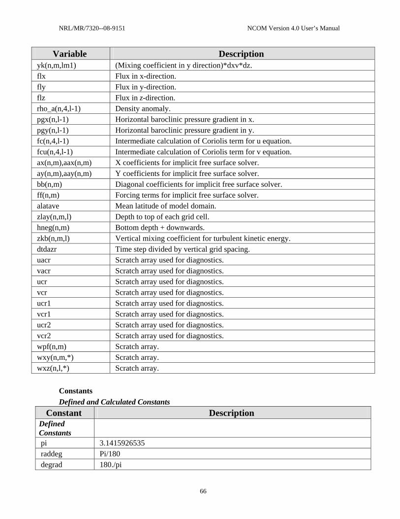
NRL/MR/7320--08-9151 NCOM Version 4.0 User’s Manual
Variable Description yk(n,m,lm1) (Mixing coefficient in y direction)*dxv*dz. flx Flux in x-direction. fly Flux in y-direction. flz Flux in z-direction. rho_a(n,4,l-1) Density anomaly. pgx(n,l-1) Horizontal baroclinic pressure gradient in x. pgy(n,l-1) Horizontal baroclinic pressure gradient in y. fc(n,4,l-1) Intermediate calculation of Coriolis term for u equation. fcu(n,4,l-1) Intermediate calculation of Coriolis term for v equation. ax(n,m),aax(n,m) X coefficients for implicit free surface solver. ay(n,m),aay(n,m) Y coefficients for implicit free surface solver. bb(n,m) Diagonal coefficients for implicit free surface solver. ff(n,m) Forcing terms for implicit free surface solver. alatave Mean latitude of model domain. zlay(n,m,l) Depth to top of each grid cell. hneg(n,m) Bottom depth + downwards. zkb(n,m,l) Vertical mixing coefficient for turbulent kinetic energy. dtdazr Time step divided by vertical grid spacing. uacr Scratch array used for diagnostics. vacr Scratch array used for diagnostics. ucr Scratch array used for diagnostics. vcr Scratch array used for diagnostics. ucr1 Scratch array used for diagnostics. vcr1 Scratch array used for diagnostics. ucr2 Scratch array used for diagnostics. vcr2 Scratch array used for diagnostics. wpf(n,m) Scratch array. wxy(n,m,*) Scratch array. wxz(n,l,*) Scratch array.
Constants Defined and Calculated Constants
Constant Description Defined Constants
pi 3.1415926535 raddeg Pi/180 degrad 180./pi
66
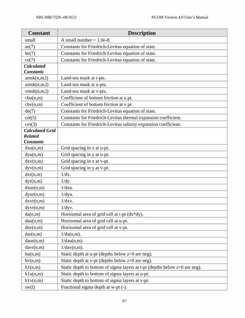
NRL/MR/7320--08-9151 NCOM Version 4.0 User’s Manual
Constant Description small A small number = 1.0e-8. ae(7) Constants for Friedrich-Levitus equation of state. be(7) Constants for Friedrich-Levitus equation of state. ce(7) Constants for Friedrich-Levitus equation of state. Calculated Constants
amsk(n,m,l) Land-sea mask at t-pts. umsk(n,m,l) Land-sea mask at u-pts. vmsk(n,m,l) Land-sea mask at v-pts. cbu(n,m) Coefficient of bottom friction at u pt. cbv(n,m) Coefficient of bottom friction at v pt. de(7) Constants for Friedrich-Levitus equation of state. cet(5) Constants for Friedrich-Levitus thermal expansion coefficient. ces(3) Constants for Friedrich-Levitus salinity expansion coefficient. Calculated Grid Related Constants
dxu(n,m) Grid spacing in x at u-pt. dyu(n,m) Grid spacing in y at u-pt. dxv(n,m) Grid spacing in x at v-pt. dyv(n,m) Grid spacing in y at v-pt. dxr(n,m) 1/dx. dyr(n,m) 1/dy. dxur(n,m) 1/dxu. dyur(n,m) 1/dyu. dxvr(n,m) 1/dxv. dyvr(n,m) 1/dyv. da(n,m) Horizontal area of grid cell at t-pt (dx*dy). dau(n,m) Horizontal area of grid cell at u-pt. dav(n,m) Horizontal area of grid cell at v-pt. dar(n,m) 1/da(n,m). daur(n,m) 1/dau(n,m). davr(n,m) 1/dav(n,m). hu(n,m) Static depth at u-pt (depths below z=0 are neg). hv(n,m) Static depth at v-pt (depths below z=0 are neg). h1(n,m) Static depth to bottom of sigma layers at t-pt (depths below z=0 are neg). h1u(n,m) Static depth to bottom of sigma layers at u-pt. h1v(n,m) Static depth to bottom of sigma layers at v-pt. sw(l) Fractional sigma depth at w-pt (-).
67

NRL/MR/7320--08-9151 NCOM Version 4.0 User’s Manual
68
Constant Description sm(l) Fractional sigma depth at t-pt (-). dsw(l) Fractional sigma grid spacing at w-pt (+). dsm(l) Fractional sigma grid spacing at t-pt (+). dswr(l) 1/dsw. dsmr(l) 1/dsm. dsm5(l) dsm/2. dzm5(l) dzm/2. zw(l) Static depth at w-pt on z-level grid (values below z=0 are neg). zm(lm1) Static depth at t-pt on z-level grid (values below z=0 are neg). dzw(l) Vertical grid spacing at w-pt (+) on z-level grid. dzm(lm1) Vertical grid spacing at t-pt (+) on z-level grid. dzwr(l) 1/dzw. dzmr(l) 1/dzm. ddx(n,m) Difference in x grid spacing in y direction, dx(i,j+1) -dx(i,j-1). ddy(n,m) Difference in y grid spacing in x direction, dy(i+1,j) -dy(i-1,j). fda(n,m) "Modified" Coriolis parameter, defined at t-pts (= f*da*0.25).