Fingerprinting of Non-resolved Three-axis Stabilized Space Objects Using a Two-Facet Analytical Model

By

Anil Bhaskar Chaudhary1, Tamara Payne1, Steve Gregory2, and Phan Dao3

1 Applied Optimization, 2 Boeing LTS,

3 AFRL Space Vehicles Directorate, Kirtland AFB, Albuquerque, NM

ABSTRACT This approach to resident space object (RSO) fingerprinting is motivated by the established framework of biometric fingerprinting which comprises a basic differentiator, followed by three levels of matching. Level 0 (L0) features would be the size and type of the fingerprint. Level 1 (L1) features are the macro characteristics of the fingerprint. Level 2 (L2) features are locations where a single ridge in the fingerprint splits into two branches or where two branches converge into one. Level 3 (L3) features describe the periodic pattern in the fingerprint. Match at each level provides progressively higher confidence. Correspondingly, the RSO fingerprinting can be considered to comprise matching at a base level, followed by three levels of features. L0 consist of sentinel features such as the gross brightness, and contrast, shape and position of principal specular glints. L1 features comprise the geometric shape of the signature brightness and its color indices. This is analytically represented using a polynomial in the cosine of the sub-solar angle, which captures the effect of the seasons. The Level 2 captures the intrinsic character of the sloping regions or bifurcations in the signature brightness and color. It is used to separate the contribution of the solar panel and body. Level 3 consists of the temporal evolution of the fractional abundance of the solar panel and the body. This allows inference on the mechanical stability and basic information about the attitude of the RSO. A collection of L0 to L3 features for an RSO is thus defines its fingerprint.

1.0: INTRODUCTION The research objective of the present work was to develop techniques for the fingerprinting of three-axis stabilized, non-resolved resident space objects (RSOs). This class of RSOs was chosen due to its growing importance in all orbits and this work has resulted in the original development of a new technique, which is based on a reduced parameter, two-facet model for the RSOs and a collection of two-point methods for RSO characterization [References 4-7]. This approach to RSO fingerprinting is motivated by the established framework of biometric fingerprinting, which consists of a basic differentiator, followed by three levels of calculations [References 1-3]. A match between two human fingerprints at each level provides a successively higher level of confidence. Figure 1 illustrates how human fingerprinting may be used as a metaphor for RSO fingerprinting. The elements of human fingerprinting are shown in black letters and the corresponding elements for RSO fingerprinting are shown in red letters. An RSO fingerprint may be defined as a collection of results from RSO characterization that can be used to distinguish one RSO from other RSOs above an acceptable threshold of confidence. It is defined to comprise matching at a base level (L0), followed by the three levels of features, L1, L2 and L3. Taken together, the fingerprinting method is denoted as the Lx technique. The Lx technique can be used for both visible spectrum and infrared data [Reference 4, 5]. It assumed that the RSO metric data is the first differentiator between the RSOs. In other words, a cross-tag between two, stable three-axis RSOs may occur if the two objects are closely spaced. The present paper covers only the visible spectrum calculations. Salient components of the Lx technique can be implemented using two, single-point brightness data points of panchromatic, multi-spectral, or hyperspectral data. The availability of extended duration signature data is not essential. This method was developed because single-point brightness is the most prevalent type of data available. Also, it extends naturally to multi-spectral or hyper-spectral data, when available.

Figure 1: Three levels in biometric fingerprinting The Lx technique uses a reduced parameter, two-facet model [Reference 4]. This results in analytical expressions which can be combined in a way that the number of unknowns in the model can be equalized to the number of independent equations [Reference 5]. This occurs under specific observation conditions that are determined based on a mathematical analysis. The resulting solution useful is for cross-tag resolution and the characterization of optical properties of RSO surface materials [References 6-7]. Furthermore, the two-facet model can be used under routine observation conditions, which can make it feasible to make the calculations repeatedly, on a daily basis if so desired, in order to quantify the bias in the solution. This paper is organized as follows: Section 2 describes the two-facet model. Section 3 provides analytical expressions for the two-facet model. Section 4 describes the Lx algorithms. A RSO fingerprint report generated using the Lx technique is given in Section 5. It is based on the use of multi-color photometry data. An example of the L2 calculation using the two-point method on panchromatic single-point brightness data is shown Section 6. The conclusions are given in Section 7.

2.0: TWO-FACET MODEL: METHOD, ASSUMPTIONS, AND PROCEDURE For RSO fingerprinting, a general observation is that the signature analysis problem consists of known variables and unknown invariants. Specifically: Known Variables and Variable Features: For a broad range of observation conditions, the temporal changes in the RSO signature occur due to the changes in the projected view of the RSO with respect to the sensor, RSO illumination conditions, and a possible, gradual articulation of the RSO geometry. These changes occur even if the RSO itself is in a steady-state operation, which would be the majority of time it is on orbit. If the RSO stabilization scheme is assumed to be known, the RSO orientation with respect to the earth and the sun is known. This orientation can be projected with respect to the sensor position. The above list of entities that cause changes in the signature is deemed ‘known variables’. Semantic features of the signature such as its brightness, color index, etc. are deemed ‘variable features’. Unknown Invariants and Invariant Features: RSO surface materials age in space. The space environment changes the surface material reflectance and absorption properties. Typically, the RSO brightness declines and temperatures rise. The extent of such dimming and warming is typically unknown. The resulting change in the signature also scales by the surface area of the RSO component. The surface area for the facets is may also be unknown. Thus, the albedo-area and emissivity-area products are unknowns that change slowly over time under nominal conditions. Their rate of change is governed by the physical laws governing the material changes due to the space environment. They are denoted as the ‘unknown invariants’. These are deemed ‘invariant features’.

A fundamental issue in RSO fingerprinting is non-uniqueness. It occurs because the number of independent equations is less than the number of unknowns. This poses itself as a rectangular system of governing equations, which needs to be solved using a minimization principle. The resulting, potential non-uniqueness is an obstacle in the extraction of actionable information. The present work seeks to overcome this difficulty by using a mathematical determination of observation conditions that equalize the number of unknowns to the number of independent equations on the basis of physical laws, electro-optic constitutive equations and geometric compatibility between observations. This is feasible because the RSO signature expression typically consists of products of the ‘known variables’ and ‘unknown invariants’. The known variables can be computed and thus are no difficulty. The approach in the present work is to solve for conditions where one or more unknown invariants have the same or related value based on a physical principle. For these conditions, algebraic manipulation of the signature expressions can equalize the number of independent equations and the number of unknowns. This results in a square, non-singular system that can provide results with insightful credence. The two-facet model is a salient component of this work, which allows a reduced parameter representation of the RSO signature behavior. This model is useful for RSO fingerprinting of three-axis stabilized satellites using visible and infrared data. It is based on the following assumptions: • The orbital elements for the three-axis stabilized satellites are known. This means that the orientation

of the ideal satellite solar panel and body is known. The solar panel is assumed to point to the sun and the body is assumed to point to nadir. The solar panel is idealized as a single facet and the body is idealized as another single facet.

• The dimensions for the solar panel and body are unknown. This has two implications. The product of

albedo and area is unknown for the solar panel and the body. The visible signature is an unknown mixture of two albedo-area products.

• The solar panel reflectance is represented by the Phong model. This model has the ability to represent

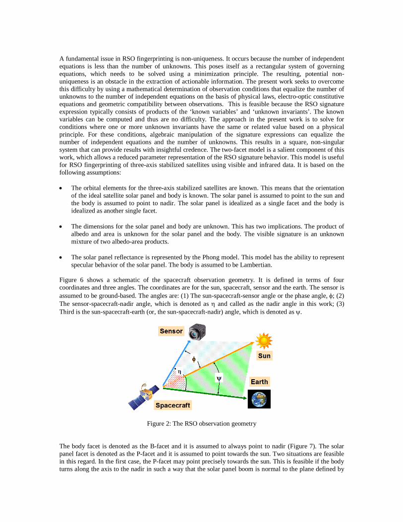
specular behavior of the solar panel. The body is assumed to be Lambertian. Figure 6 shows a schematic of the spacecraft observation geometry. It is defined in terms of four coordinates and three angles. The coordinates are for the sun, spacecraft, sensor and the earth. The sensor is assumed to be ground-based. The angles are: (1) The sun-spacecraft-sensor angle or the phase angle, φ; (2) The sensor-spacecraft-nadir angle, which is denoted as η and called as the nadir angle in this work; (3) Third is the sun-spacecraft-earth (or, the sun-spacecraft-nadir) angle, which is denoted as ψ.

Figure 2: The RSO observation geometry The body facet is denoted as the B-facet and it is assumed to always point to nadir (Figure 7). The solar panel facet is denoted as the P-facet and it is assumed to point towards the sun. Two situations are feasible in this regard. In the first case, the P-facet may point precisely towards the sun. This is feasible if the body turns along the axis to the nadir in such a way that the solar panel boom is normal to the plane defined by

coordinates of the center of the earth, RSO and the sun. The second case when the P-facet points to the sun with a small offset angle. The assumption in the two-facet model is that the solar panel offset with respect to the sun is small. The analytical calculations using the model can then be performed either when the offset is zero or when it is small. If the size of the solar panels were known, the area of the P-facet would equal the total area of the solar panels. Figure 8 shows a simplistic 2D illustration of the model, which is useful for getting a physical insight and visualizing the mathematics. The P-facet is shown as a blue line and the B-facet is shown as an orange line. Such a planar geometry could occur, but only rarely.

Figure 3: Two-facet Model

Figure 4: 2D schematic of the two-facet model

2.1: STRENGTH, WEAKNESS AND THE USE OF THE TWO-FACET MODEL. Strength of the two-facet model: This model captures the basic truth about the orientation of 3-axis stabilized RSOs that the solar panel points to the sun and the body points to nadir. It also represents a basic truth about the solar panel that its geometry is essentially flat and thus it is represented with a single planar facet. It allows representation of specular behavior of the solar panel, which is a dominant contribution to the visible signature. The model allows analytical formulation for the visible signature and allows transparency in the mathematical manipulations, lending itself to the determination of simple thumb rules for analysis of RSO signature data as well as planning of future observations.

P

B

Solar Panel

Body

Weakness of the two-facet model: The body is represented as a single planar facet. The body is a solid object and can have complex attachments. The body is represented as Lambertian in order to reduce the number of unknowns. Use of a single facet to represent the body creates a limitation that the non-symmetry in the signature due the illumination of the body from different sides cannot be reproduced by the model. Use of the two-facet model: The orientation of the two facets is computed using an orbital calculation program and the protocol for three-axis stabilization. This provides the necessary input data for the formulation of the analytical equations to represent the RSO signature. The various calculations needed in order to perform RSO fingerprinting can be performed using supplemental software utility programs. Indeed, several signature analysis calculations can even by performed using a desk calculator once the two-facet orientation is known.

2.2: PHONG MODEL FOR THE SOLAR PANEL (P-FACET)

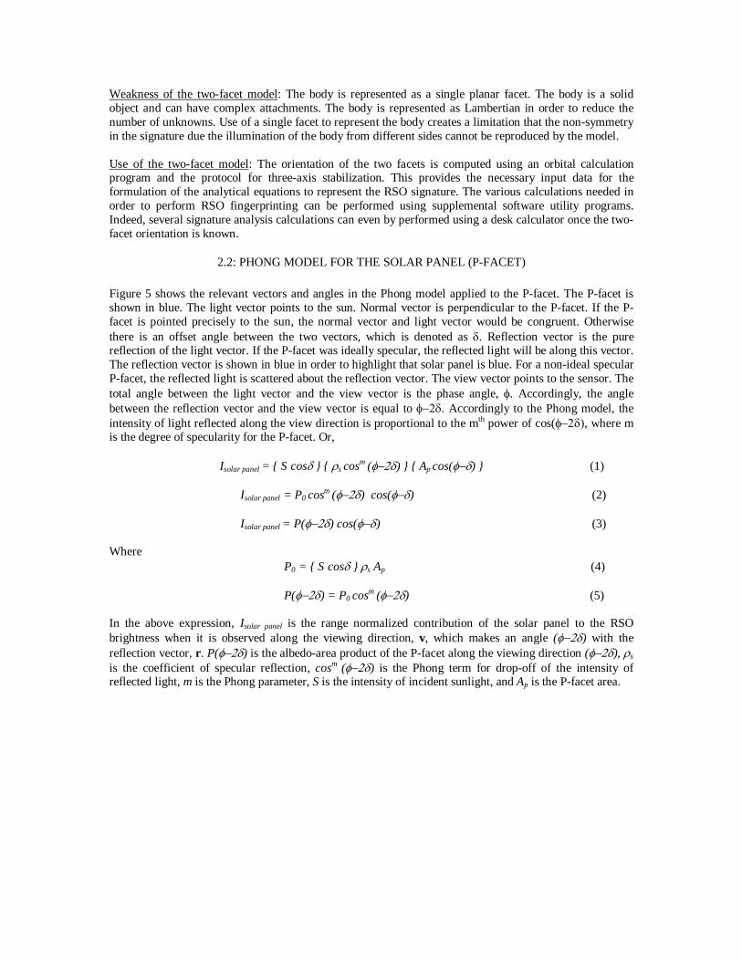
Figure 5 shows the relevant vectors and angles in the Phong model applied to the P-facet. The P-facet is shown in blue. The light vector points to the sun. Normal vector is perpendicular to the P-facet. If the P-facet is pointed precisely to the sun, the normal vector and light vector would be congruent. Otherwise there is an offset angle between the two vectors, which is denoted as δ. Reflection vector is the pure reflection of the light vector. If the P-facet was ideally specular, the reflected light will be along this vector. The reflection vector is shown in blue in order to highlight that solar panel is blue. For a non-ideal specular P-facet, the reflected light is scattered about the reflection vector. The view vector points to the sensor. The total angle between the light vector and the view vector is the phase angle, φ. Accordingly, the angle between the reflection vector and the view vector is equal to φ−2δ. Accordingly to the Phong model, the intensity of light reflected along the view direction is proportional to the mth power of cos(φ−2δ), where m is the degree of specularity for the P-facet. Or, Isolar panel = { S cosδ } { ρs cosm (φ−2δ) } { Ap cos(φ−δ) } (1)

Isolar panel = P0 cosm (φ−2δ) cos(φ−δ) (2)

Isolar panel = P(φ−2δ) cos(φ−δ) (3) Where P0 = { S cosδ } ρs Ap (4)

P(φ−2δ) = P0 cosm (φ−2δ) (5) In the above expression, Isolar panel is the range normalized contribution of the solar panel to the RSO brightness when it is observed along the viewing direction, v, which makes an angle (φ−2δ) with the reflection vector, r. P(φ−2δ) is the albedo-area product of the P-facet along the viewing direction (φ−2δ), ρs is the coefficient of specular reflection, cosm (φ−2δ) is the Phong term for drop-off of the intensity of reflected light, m is the Phong parameter, S is the intensity of incident sunlight, and Ap is the P-facet area.

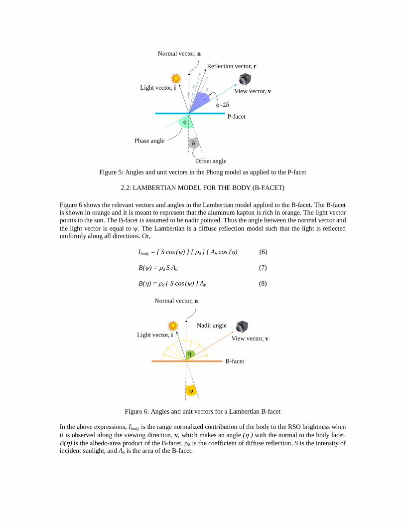
Figure 5: Angles and unit vectors in the Phong model as applied to the P-facet

2.2: LAMBERTIAN MODEL FOR THE BODY (B-FACET) Figure 6 shows the relevant vectors and angles in the Lambertian model applied to the B-facet. The B-facet is shown in orange and it is meant to represent that the aluminum kapton is rich in orange. The light vector points to the sun. The B-facet is assumed to be nadir pointed. Thus the angle between the normal vector and the light vector is equal to ψ. The Lambertian is a diffuse reflection model such that the light is reflected uniformly along all directions. Or,

Ibody = { S cos (ψ) } { ρd } { Ab cos (η) (6)

B(ψ) = ρd S Ab (7)

B(η) = ρd { S cos (ψ) } Ab (8)

Figure 6: Angles and unit vectors for a Lambertian B-facet In the above expressions, Ibody is the range normalized contribution of the body to the RSO brightness when it is observed along the viewing direction, v, which makes an angle (η ) with the normal to the body facet. B(η) is the albedo-area product of the B-facet, ρd is the coefficient of diffuse reflection, S is the intensity of incident sunlight, and Ab is the area of the B-facet.

Normal vector, n

View vector, v

Reflection vector, r

Light vector, i

P-facet

Phase angle

φ

Offset angle

δ

φ−2δ

Normal vector, n

View vector, vLight vector, iNadir angle

ψ

B-facetη

3.0: ANALYTICAL EXPRESSION FOR RANGE-NORMALIZED VISUAL BRIGHTNESS Figure 7 shows the application of the two-facet model for the analysis of visual brightness. The P-facet is represented by the Phong model and the B-facet is Lambertian. The analytical expression for the visual brightness is given by:

Ik(tj) = Pk(φj-2δ) cos(φj−δ) + Bk(ψj) cosψj cosηj (9) Where Ik(tj) is the single point RSO brightness at time ‘t’ in a waveband ‘k’. Occurrences of the subscript ‘j’ denote a particular instant of time. If the data is observed in n wavebands, there will be n equations of the same form. The angles φ, ψ, and η are the phase angle, nadir angle, and the sun-RSO-earth angle at time t. Pk(φ−2δ) is the albedo-projected area product of the P-facet at phase angle φ and offset δ in waveband k. Typically Pk(φ−2δ) becomes larger as (φ−2δ) becomes smaller. This is because the P-facet has a specular behavior. The Bk(ψ) is the albedo-area product of the B-facet in waveband k.

Figure 7: Observation trigonometry

Note that for each waveband, there is a single independent equation for the visual spectrum brightness, Ik(j). This equation contains two unknowns Pk(φ−2δ) and Bk(ψ). Thus there is one extra unknown per equation and it is not feasible to solve for Pk(φ−2δ) and Bk(ψ), except under special conditions when (φ−δ) equals 90o or either one of angles ψ and η is 90o. Considering a ground-based sensor, η cannot equal 90o. Angles (φ−δ) and ψ can be 90o, and this can provide useful information for RSO fingerprinting. If the RSO brightness was observed in n-wavebands, the situation does not change. This is because the number of independent equations is equal to n and the number of unknowns is equal 2n. This is because the values of Pk(φ−2δ) and Bk(ψ) depend on the waveband. This is a basic difficulty in calculating the individual contribution of the P-facet and B-facet. The present work provides a way to circumvent this difficulty, which is described in the following sections. Sign of the phase angle: The methods described in the following sections make use of the sign of the phase angle. This sign is defined using triple product of three vectors; namely the light vector i, view vector v, and the vector z, which points to the celestial north.

𝑡𝑟𝑖𝑝𝑙𝑒 𝑝𝑟𝑜𝑑𝑢𝑐𝑡 = 𝒊 ∙ ( 𝒛 × 𝒗 ) (10) If the triple product is greater than zero, the phase angle (i.e. the angle between the vectors i and v) is denoted as positive. If the triple product is negative, the phase angle is denoted as negative (see Figure 12). The choice of assigning a positive or negative sign to the phase angle as per the sign of the triple product is arbitrary. It could be defined vice versa.

Phase Angle

φ

Sensor

ψ η

P

Nadir Angle

BP

B

i

v

3.1: COMMON FEATURES OF VISUAL SIGNATURES The purpose of this section is to note the features of visual signatures that are determined based on the analytical form of the range-normalized visual brightness. In order to complement the analytical explanation, Figure 8 shows a plot of six signatures in the Johnson-B band for a geosynchronous satellite. They are denoted as G1, G2, G3, etc. They are shown in order to illustrate the rationale behind the hypotheses. This is a GEO satellite and it was observed from the same ground-based. It has two solar panels and a complex body. The plot shows the signature brightness as a function of the phase angle. Since the two-facet model is a reduced parameter model, it cannot explain the small, local undulations that are present in the signature, which can arise due to specular glints from small features, self-occlusion, etc. However, the simplicity of the model lends itself to physical insight using simple arguments. For this purpose, it is convenient to modify the range-normalized expression for visual brightness by cos(φj−δ) as follows. This range and cos(φj−δ) normalized expression is denoted as Jk(t). The subscript j denotes an instant of time.

𝐼𝑘�𝑡𝑗�

cos�𝜙𝑗−𝛿�= 𝑃𝑘�𝜙𝑗 − 2𝛿�+

𝐵𝑘�𝜓𝑗� 𝑐𝑜𝑠𝜓𝑗 𝑐𝑜𝑠𝜂𝑗cos�𝜙𝑗−𝛿�

(9)

𝐽𝑘(𝑡𝑗) = 𝐼𝑘�𝑡𝑗�

cos�𝜙𝑗−𝛿� (10)

It is known that when the phase angle equals twice the offset angle, or φ = 2δ, the signature brightens significantly due to the specular glint. This is when the phase angle bisector condition is met. As the phase angle increases, the signature becomes dimmer.

Figure 8: Six Signatures in the Johnson-B Band Note 1: The contribution of the solar panel to the normalized brightness, Jk(t), is symmetric about the specular glint that occurs when φ = 2δ . This shape and character of this symmetric contribution is governed by the Phong term, cosm (φ−2δ). Note 2: The shape of the specular peak at φ = 2δ is typically not symmetric. The balance of the signature is also not symmetric about the specular peak. This can be observed by folding the signature about the specular peak (Figure 9). This creates an overlap of the signatures from the regions where the angle (φ−2δ) is positive and negative. Such folding can be performed automatically by plotting the signature with respect to cos(φ−2δ). The folded signature has two branches that meet at the specular peak.

6

8

10

12

14

-45 -25 -5 15 35Phase Angle

Visu

al M

agni

tude

G1G2G3G4G5G6

2*Phase Angle Offset, or 2δ

Figure 9: Folded Signatures in Johnson B-Band versus cos (φ − 2δ)

Note 3: Assume that the specular peak occurs over a narrow interval of the phase angle. In this interval, assume that the rate of the change of body contribution is constant. The rate of change of solar panel signature is positive on one side of the peak and negative on the other side of the peak. Thus, with respect to the specular peak, the rate of the change of body contribution is an even function and the rate of change of the solar panel contribution is an odd function. Note 4a: The sum of the signature slope just before the specular peak and just after the specular peak is equal to twice the rate of change of signature due to B-facet. This is because the contribution of the solar panel cancels out.

Note 4b: The difference between the slope of the signature before and after the specular peak equals twice the rate of change of signature due to the P-facet. This is because the body contribution cancels out. Note 4c: Let the visual signature data be available in n-wavebands. Then the rate of change of signature due to the B-facet and P-facet can be calculated as per Notes 4a and 4b for each of n-wavebands independently of each other. The result is the multi-spectral rate of change of signature by the B-facet and P-facet adjacent to the specular peak. This multi-spectral rate of change can be normalized in order to obtain the normalized reflectance spectrum for the B-facet and P-facet. This is fundamentally useful information. Note 5: When the angle (φ - 2δ) becomes large, the rate of change of the solar panel contribution becomes small. Or, the term P(φ−2δ) is nearly constant for small changes in the phase angle. Consider two time values, tj and tm , when the magnitude of (φ−2δ) is large. Then the change in the normalized signature, ( Jk(tj) - Jk(tm) ) is due to the change in the body contribution. Note 6a: Consider two instances of time tj and tm when the magnitude of (φ−2δ) is equal. At these instances, the values of Jk(tj) and Jk(tm) are typically not equal to each other. The analytical expressions for the visual brightness can be utilized in order to determine the albedo-area product of the B-facet from panchromatic, multi-spectral and hyperspectral data. This observation is a first tenet of the two-point method reported in Section 4.3.2. Note 6b: The calculation of Note 6a can be repeated for multiple different pairs of time values (or pairs of two-points) in order to obtain the albedo-area product of the B-facet as a function of angle ψ. This is fundamental to the material characterization of the B-facet. Note 7a: The procedure for the determination of the P-facet albedo-area can be visualized by considering another normalization of the visual brightness expression in Equation (9).

𝐼𝑘�𝑡𝑗�

𝑐𝑜𝑠𝜓𝑗 𝑐𝑜𝑠𝜂𝑗=

𝑃𝑘�𝜙𝑗−2𝛿� cos�𝜙𝑗−𝛿�

𝑐𝑜𝑠𝜓𝑗 𝑐𝑜𝑠𝜂𝑗+ 𝐵𝑘�𝜓𝑗� (11)

7

9

11

13

150.7 0.8 0.9 1

Visu

al M

agni

tude

G1G2G3G4G5G6

cos(φ – 2δ)

𝐿𝑘(𝑡𝑗) = 𝐼𝑘�𝑡𝑗�

𝑐𝑜𝑠𝜓𝑗 𝑐𝑜𝑠𝜂𝑗 (12)

Now consider two instances of time tj and tm that have the same value of angle ψj. At these instances, the values of Lk(tj) and Lk(tm) are typically not equal to each other. This difference ( Lk(tj) - Lk(tm) ) is due to the difference in the contribution of the P-facet. With this observation, the analytical expressions for the visual brightness can be utilized in order to determine the albedo-area product of the P-facet from panchromatic, multi-spectral and hyperspectral data. This observation is a second tenet of the two-point method reported in Section 4.3.2.3. Note 7b: The calculation of Note 7a can be repeated for multiple different pairs of time values (or pairs of two-points) in order to obtain the albedo-area product of the P-facet as a function of angle (φ - 2δ). This is fundamental to the material characterization of the P-facet. Note 7c: If the values of Phong parameter, m, and the solar panel offset angle, δ, are unknown, the analytical calculations can be set up in order to determine these parameters from single point brightness data at time instances defined as per a mathematical calculation.

4.0: Lx FINGERPRINTING ALGORITHMS The Lx technique consists of the L0, L1, L2 and L3 components, which are described in this section.

4.1: L0 – SENTINEL FEATURES The prominent attributes of the RSO signature that can be described in conversational English are denoted as the sentinel features. Some of the sentinel features may be observable only under special observation conditions that are not encountered under routine tasking. For example, the location of a specular peak typically occurs at a small, nonzero phase angle where the phase angle bisector condition is fulfilled. The location, width and contrast of the specular peak are examples of sentinel features (see Section 5.1).

4.2: L1 – VARIABLE FEATURES The purpose of the L1 features is to capture the macro character of the RSO signature under routine observation tasking. An important challenge in the definition of the L1 features is that the RSO signature depends on the observation geometry and the seasons. A common practice is to consider the phase angle as a single variable. However, the nature of the phase angle dependency is complex and it relies on its two-dimensional quality: the longitudinal or equatorial plane of the phase angle and the latitudinal plane of the phase angle, which are coplanar with the Earth’s longitude and latitude respectively. This is illustrated in Figure 10 for a geosynchronous (GEO) satellite. The figure shows three sets of multi-spectral signatures were collected at different times of the year, i.e. different solar latitudinal angles. Each signature was collected roughly during the same times of the night, i.e. similar solar longitudinal angles, which is plotted on the x axis of each signature plot. The signatures are quite different from each other. These differences may be considered as bounds because the signatures are collected at the equinox, and the summer and winter solstice conditions whereby the subsolar angle changes from -23.5o to +23.5o. The algorithm for the L1 features seeks to account for the effect of the subsolar angle and the phase angle on the RSO signature or its single point brightness by synthesizing the historical archive of RSO photometry observations data into a single representation. The historical archive is viewed as a table of RSO brightness versus phase angle and subsolar angle. Or, the data is represented as I(φ, ζ), where φ and ζ are the phase angle and the subsolar angle, respectively. The goal is to combine this information such that the visual brightness values can be interpolated at any phase angle on any day of the year (i.e. for a given value of the subsolar angle). A polynomial in the cosine of the subsolar angle is used as the basis function for this purpose. This function is reminiscent of the Limaçon, which is defined using a linear term in the cosine. The definition of the L1 features uses a quadratic polynomial in the cosine for the interpolation and

visualization of a signature archive. The polynomial function is defined in terms of a cylindrical coordinate system as shown in Figure 11. The standard brightness versus phase angle plots, or “signatures” are plotted along the z axis, where the brightness is a function of the phase angle. The radial axis distance is the corresponding brightness and the polar angle is a measure of the solar declination (subsolar angle) by ordinal date (day of the year) ranging from 0 to 365. The Limaçon function expresses the visual brightness as a quadratic polynomial given by: I(φ,ζ) = b(φ) + a(φ) cos ζ + c(φ) cos2ζ. Note that this is an even function that fulfills the character of the change in the illumination conditions at the equinox and solstice.

Figure 10: Multi-spectral signatures of a GEO satellite taken under different seasonal conditions

Figure 11: The polar coordinate frame used in the definition of the L1 features

7

8

9

10

11

12

13

14

15

-60 -45 -30 -15 0 15 30 45 60 75 90 105 120Phase Angle

Visu

al M

agni

tude

Band-BBand-RBand-I

7

8

9

10

11

12

13

14

15

-60 -45 -30 -15 0 15 30 45 60 75 90 105 120Phase Angle

Visu

al M

agni

tude

Band-BBand-VBand-I

7

8

9

10

11

12

13

14

15

-60 -45 -30 -15 0 15 30 45 60 75 90 105 120Phase Angle

Visu

al M

agni

tude

Band-BBand-VBand-RBand-I

Z axis, phase angle in longitudinal plane(0:360) – “Right Ascension”

Radial axis distance,brightness orcolor in magnitude

Radial axis angle, phase angle in latitudinal plane(Ordinal date - 0:365) – “Declination”

Jan (0)Jun (180)

4.2.1: PROCEDURE FOR THE GENERATION OF THE L1 FEATURE (LIMAÇON PLOT) The L1 plot is generated using the following seven steps: (1) Organize the available signatures in the desired band or color index by the ordinal date of its

collection. The range of ordinal dates is [0, 365]. (2) Map the ordinal date to the subsolar angle. The ordinal dates from the winter solstice to vernal

equinox to summer solstice are mapped to the range of subsolar angles, ζ, from [-23.5o to 23.5o]. The ordinal dates from the summer solstice to autumnal equinox to winter solstice are mapped to the range of subsolar angles, ζ, from [23.5o, -23.5o].

(3) Define another angle, ξ ,such that:

For ordinal dates from winter solstice to vernal equinox to summer solstice

ξ = {180/(2∗23.5)}{ 23.5 + ζ } (13)

This maps the angle ζ to the values of ξ in the range [0, 180]

For ordinal dates from summer solstice to autumnal equinox to winter solstice

ξ = {180/(2∗23.5)}{ 23.5 − ζ } + 180 (14) This maps the angle ζ to the values of ξ in the range [180, 360]

(4) Represent the Limaçon as a polynomial I(φ,ξ) = b(φ) + a(φ) cos ξ + c(φ) cos2 ξ (5) Define a resolution, ∆φ. This means that the Limaçon is to be fitted to the signature data at phase angle

values of ∆φ, 2∆φ, 3∆φ, 4∆φ, etc. (6) The signature or single point data will typically not be available at the desired level of resolution, ∆φ. It

may be available at the phase angle values of φ1, φ2, φ3, φ4, φ5, etc. Interpolate the available data to the phase angle values of ∆φ, 2∆φ, 3∆φ, 4∆φ, etc.

(7) Fit the Limaçon polynomial to the signature data at each phase angle separately. The Limaçon polynomial has three parameters and thus a minimum of three data points are needed at each phase angle. The three points may be interspersed over the range of permissible values of ξ from [0, 360].The values for the three parameters are determined using least squares. This results in a sequence of values for parameters b(φ), a(φ) and c(φ) at a resolution level of ∆φ. Use these parameters to create the Limaçon plot, which captures the macro character of the RSO brightness, I(φ,ζ).

The benefit of the L1 Limaçon plot is that it can be used to compare the Limaçon plots for two RSOs in order to determine the (φ,ζ) regions two RSOs have similar brightness and the the (φ,ζ) regions two RSOs are dissimilar. This is useful information for the purposes of space object identification. The L1 features are considered variable features because they are a function of the angles (φ,ζ).

4.3: L2 – INVARIANT FEATURES RSO brightness is a function of the illumination conditions, observation geometry and the albedo-area products for the solar panel and the body. The illumination conditions and observation geometry change significantly, causing significant changes in the signature. These changes can be computed for a three-axis stabilized RSO based on its orbital position and time. The area of RSO components (e.g. body and the solar panel) is constant. The albedo is a function of material reflectance properties, which change on a time scale of years. Thus, one may consider the RSO signature to be product-sum of known entities that change quickly and unknown entities that are practically invariant. The purpose of the L2 calculation is to solve for the invariant entities or features. The invariant information (albedo-area product) for the solar panel and body is fundamental to understanding the material content of a RSO signature. Consider that an RSO is observed over a period of time by different sensors. When a specular glint is observed, the material reflectance spectrum can be extracted. Since a glint can be observed repeatedly, the

reflectance spectrum can be independently verified. Collection of all reflectance spectra for an RSO can become an archive of known information about its signature. If the material spectra are compared with its older values, it provides information on how the material spectrum is changing, or how the B-facet and P-facet materials are aging in orbit. Furthermore, the material spectra can be used as input for temporal unmixing of the RSO signatures, which is a part of the L3 calculations. The notes 4 to 6 in Section 3.1 state a procedure for the determination of the normalized values of the spectral albedo-area product for the P-facet and B-facet. The method described in this section is for the determination of the actual value of the spectral albedo*area products.

4.3.1: CONCEPT OF GEOMETRIC COMPATIBILITY.

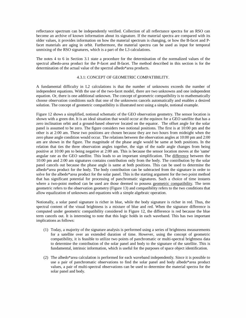
A fundamental difficulty in L2 calculations is that the number of unknowns exceeds the number of independent equations. With the use of the two-facet model, there are two unknowns and one independent equation. Or, there is one additional unknown. The concept of geometric compatibility is to mathematically choose observation conditions such that one of the unknowns cancels automatically and enables a desired solution. The concept of geometric compatibility is illustrated next using a simple, notional example. Figure 12 shows a simplified, notional schematic of the GEO observation geometry. The sensor location is shown with a green dot. It is an ideal situation that would occur at the equinox for a GEO satellite that has a zero inclination orbit and a ground-based observer located on the equator. The offset angle for the solar panel is assumed to be zero. The figure considers two notional positions. The first is at 10:00 pm and the other is at 2:00 am. These two positions are chosen because they are two hours from midnight when the zero phase angle condition would occur. The relations between the observation angles at 10:00 pm and 2:00 am are shown in the figure. The magnitude of the phase angle would be same at both positions. In the relation that ties the three observation angles together, the sign of the nadir angle changes from being positive at 10:00 pm to being negative at 2:00 am. This is because the sensor location moves at the 'same' angular rate as the GEO satellite. This leads to an important simplification. The difference between the 10:00 pm and 2:00 am signatures contains contribution only from the body. The contribution by the solar panel cancels out because the phase angle is same at both positions. This can be used to determine the albedo*area product for the body. The body contribution can be subtracted from the signature in order to solve for the albedo*area product for the solar panel. This is the starting argument for the two point method that has significant potential for processing of panchromatic signatures. Such a choice of time instants where a two-point method can be used are those deemed to possess geometric compatibility. The term geometric refers to the observation geometry (Figure 13) and compatibility refers to the two conditions that allow equalization of unknowns and equations with a simple algebraic operation. Notionally, a solar panel signature is richer in blue, while the body signature is richer in red. Thus, the spectral content of the visual brightness is a mixture of blue and red. When the signature difference is computed under geometric compatibility considered in Figure 12, the difference is red because the blue term cancels out. It is interesting to note that this logic holds in each waveband. This has two important implications as follows:

(1) Today, a majority of the signature analysis is performed using a series of brightness measurements for a satellite over an extended duration of time. However, using the concept of geometric compatibility, it is feasible to utilize two points of panchromatic or multi-spectral brightness data to determine the contribution of the solar panel and body to the signature of the satellite. This is fundamental, intrinsic information, which is useful for the purposes of space object identification.

(2) The albedo*area calculation is performed for each waveband independently. Since it is possible to

use a pair of panchromatic observations to find the solar panel and body albedo*area product values, a pair of multi-spectral observations can be used to determine the material spectra for the solar panel and body.

Figure 12: Illustration of geometric compatibility using the RSO positions 10:00 pm and 2:00 am In order to calculate the contribution of the P-facet and B-facet, the simplified treatment of Figure 12 needs to be modified because the GEO satellites commonly orient their solar panels with a nonzero offset angle. This offset changes the GEO Observation geometry and the magnitude of the signature observed at the same ground-based site at the notional 10:00 pm and 2:00 pm positions. The method needed to account for the nonzero offset angle is described next.

4.3.2: TWO-POINT METHOD Figure 12 illustrated one type of geometric compatibility. There are different ways in which the geometric compatibility can be applied and it results in a number of variants of the two point methods. They share a common theme. Two compatible points of data is condensed to eliminate one unknown. If there are two unknowns to be solved for, then the two-method is applied twice. In other words, in order to solve for two unknowns, four data points, selected to fulfill geometric compatibility are chosen.

4.3.2.1: METHOD 1: SOLVING FOR THE NORMALIZED MATERIAL SPECTRUM FOR THE B-FACET

This calculation is based on Note 5 in Section 3.1. Consider two points where the absolute value of the angle (φ-2δ) is large. Let the two points be denoted as tj and tm. Then,

)cos(cos)cos()(

)cos(cos)cos()(

)()(δφ

ηψψδφ

ηψψ−

−−

=−m

mmk

j

jjkmkjk

BBtJtJ (15)

The right hand side of equation (35) is only a function of B-facet parameters. If this calculation is repeated for each waveband, the right hand side is obtained for each waveband. This resulting vector of values can be normalized (i.e., scaled such the maximum value for any element of the vector equals one) to obtain the normalized material reflectance spectrum for the B-facet. This calculation requires the knowledge of the offset angle, δ. Furthermore, since the two-facet model cannot reproduce the fine features of the signature, the normalized material spectrum obtained from one set of two points may vary from another set of two points. This is particularly so if the data is noisy. It is, however, observed that if the calculation is repeated

B B

P

φφ

ψ ψ

η η

Shad

ow

P

BB BB

PP

φφ

ψ ψ

ηη η

Shad

ow

PP

φ ψ η= -

ψ φ η= +

φ ψ η= -

ψ φ η= +

φ ψ η= -φ ψ η= -

ψ φ η= +ψ φ η= +

φ ψ η= +

ψ φ η= -

φ ψ η= +φ ψ η= +

ψ φ η= -ψ φ η= -

for all eligible sets of two points, then a clear trend emerges, which may be chosen as the normalized material spectrum for the body. An important point to note is that this calculation can be performed under ordinary observation conditions and can thus be readily repeated. The material reflectance spectrum, thus calculated, can be verified repeatedly and by independent observers.

4.3.2.2: METHOD 2: SOLVING FOR THE NORMALIZED MATERIAL SPECTRUM FOR THE P-FACET

This calculation is based on Note 4b in Section 3.1. Consider the two sides of the specular peak. Let one side to be the ascending side and the other side to be the descending side. Also consider the following derivative along the ascending and the descending side:

)2cos()(

cos)cos()cos()2(

)2cos()2cos()(

δφηψδφδφ

δφδφ −+

−−−

=− d

tdBPd

dd

tdL kkk (16)

ascending

kPd

d

−−− ηψ

δφδφδφ cos)cos(

)cos()2()2cos(

descending

kPd

d

−−−

−ηψ

δφδφδφ cos)cos(

)cos()2()2cos(

(17)

The right hand side of the difference in slope of the ascending and descending side of the specular peak is only a function of the P-facet material spectrum, based on the assumption that the rate of change of B-facet contribution is constant over the interval of the phase angle where the specular peak is encountered. The use of this method needs signature data about the location where the specular peak occurs.

4.3.2.3: METHOD 3: SOLVING FOR B-FACET AND P-FACET CONTRIBUTION FROM SINGLE POINT BRIGHTNESS DATA

The methods 1 and 2 cannot be used with single-color signature data because the normalization is not feasible. (It is a pathological case since the computed vectors in Equations 15 and 17 have a length equal to one, or are scalars). This is the purpose of the development reported in this section. The calculation assumes that the solar panel offset angle, δ, is known (see the notes at the end of this section). Figure 13 shows the non-symmetry caused by the solar panel offset angle. Once again it considers a notional case of a geostationary orbit and that the data is collected at the equinox. The figure shows the 10:00 pm and 2:00 am positions of the RSO represented by a two-facet model. The B-facet is nadir pointed, but the P-facet has a nonzero offset angle. At the 10:00 pm position, the reflection vector off the P-facet is at an angle of (φ+2δ) from the view vector (also see Figure 12). At the 2:00 am position, the reflection vector from the P-facet is at an angle of (φ -2δ) from the view vector.

=−

−− descending

k

ascending

k

dtdL

dtdL

)2cos()(

)2cos()(

δφδφ

Figure 13: Non-symmetry caused by the nonzero solar panel offset angle, δ

The formulation of the two-point method is easier if the geometry compatibility is defined in terms of two time instants for observations where the angle ψ is same (or in terms of Figure 13, when ψ1 = ψ2= ψ). For such two points, the corresponding two visual brightness equations are:

ηψψδφδφ coscos)()cos()2()( 111 kkk BPtI +++= (18)

ηψψδφδφ coscos)()cos()2()( 222 kkk BPtI +−−= (19)

When these two equations are subtracted from each other, the B-facet term drops out, but the two unknowns still remain, namely Pk(φ1+2δ) and Pk(φ2-2δ). A Taylor series expansion is used in order to relate the two unknowns as follows:

221 φφ

φ+

= 2

21 φφφ

−=∆ (20)

)2(cos)2()2( 01 δφφδφφδφ +∆+=+∆+=+ m

kk PPP (21)

++∆++∆+= 2

2

2

0 )2(cos21)2(coscos δφ

φφδφ

φφφ

dd

ddP

mmm

(42) Taking only the linear terms yields the approximation

[ ]φδφφδφ tan)2(1cos)2( 01 +∆−≈+ mPP mk (22)

[ ]φδφφδφ tan)2(1cos)2( 02 +∆+≈− mPP m

k (23)

B

B φ1φ2

ψ2 ψ1

η

Shad

ow

PPδ

2δ

δ

2δφ2 = ψ2−η φ1 = ψ1+η

The absolute value of φ is shown in the tangent expression. This is because the phase angle is assigned a positive or negative sign as defined in Equation 10. This sign is for ease of interpretation of observation conditions only. Since tangent is an odd function, the use of sign for the phase angle creates a conflict. (The sign is not needed in the present calculations) The brightness difference between the two points of observation is given by:

[ ] )cos(tan)2(1cos)()( 021 δφφφδφφ +∆++∆−≈− mPtItI mkk

[ ] )cos(tan)2(1cos0 δφφφδφφ −∆−+∆+− mP m (24)

The above equation has three unknowns, P0, m and δ. If the solar panel offset angle δ, and the Phong parameter m, are known a priori, the above equation can be used to solve for P0. The value of P0 is back-substituted to calculate the contributions of the P-facet and the B-facet. The above calculation assumed that the values of δ and m are known. This may not always be the case. However, once δ and m are determined, they can be used repeatedly, except for periodic recalibration of their values. Section 4.3.2.4 describes an application of the two-point method for the case when δ is known but m is unknown. The offset angle δ can be determined using multiple techniques given next:

• One way to determine δ is to collect a panchromatic signature in the phase angle interval where the specular glint is likely to occur. Such data can be readily collected using a commercial-off-the-shelf ground-based telescope. The specular peak occurs at φ = 2δ.

• For RSOs that have been on orbit for several months, the value of δ can be estimated from the single point brightness data collected by the SSN sensors. The L1 Limaçon technique may be utilized in order to synthesize the archive of data for the RSO by the ordinal date and the phase angle. This helps locate the dominant specular peak and consequently the offset angle, δ.

• It is feasible to set up a two-point method for the calculation of δ using a space-based SSN sensor that collects single point brightness data.

4.3.2.4: METHOD 4: SOLVING FOR B-FACET AND P-FACET CONTRIBUTION FROM SINGLE POINT PANCHROMATIC BRIGHTNESS

This calculation requires an application of the two-point method twice. Or, it needs four points that are chosen based on the mathematical calculation in order to obtain the B-facet and P-facet contribution when the value of m is unknown. Method 1 in Section 4.3.2.3 solved for one unknown, P0. This method solves for two unknowns, P0 and m. It uses two pairs of two-points, as shown in Figure 14. Points 1 and 3 comprise the first pair. Points 2 and 4 are the second pair. The two geometric compatibility conditions for the four points are that the angles ψ1 and ψ2 are equal and the angles ψ3 and ψ4 are equal.

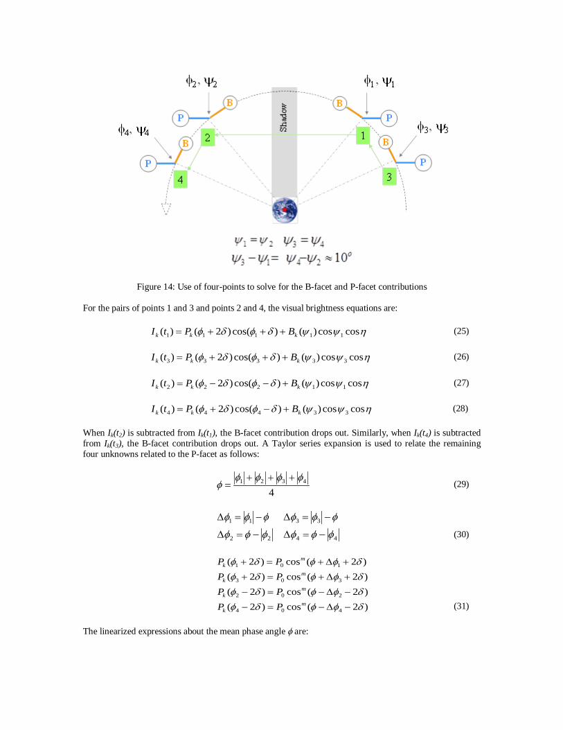
Figure 14: Use of four-points to solve for the B-facet and P-facet contributions For the pairs of points 1 and 3 and points 2 and 4, the visual brightness equations are:

ηψψδφδφ coscos)()cos()2()( 11111 kkk BPtI +++= (25)

ηψψδφδφ coscos)()cos()2()( 33333 kkk BPtI +++= (26)

ηψψδφδφ coscos)()cos()2()( 11222 kkk BPtI +−−= (27)

ηψψδφδφ coscos)()cos()2()( 33444 kkk BPtI +−+= (28) When Ik(t2) is subtracted from Ik(t1), the B-facet contribution drops out. Similarly, when Ik(t4) is subtracted from Ik(t3), the B-facet contribution drops out. A Taylor series expansion is used to relate the remaining four unknowns related to the P-facet as follows:

44321 φφφφ

φ+++

= (29)

φφφ −=∆ 11

φφφ −=∆ 33

22 φφφ −=∆

44 φφφ −=∆ (30)

)2(cos)2( 101 δφφδφ +∆+=+ m

k PP )2(cos)2( 303 δφφδφ +∆+=+ m

k PP

)2(cos)2( 202 δφφδφ −∆−=− mk PP

)2(cos)2( 404 δφφδφ −∆−=− mk PP (31)

The linearized expressions about the mean phase angle φ are:

[ ]φδφφδφ tan)2(1cos)2( 101 +∆−=+ mPP mk

[ ]φδφφδφ tan)2(1cos)2( 303 +∆−=+ mPP mk

[ ]φδφφδφ tan)2(1cos)2( 202 +∆+=− mPP mk

[ ]φδφφδφ tan)2(1cos)2( 404 +∆+=− mPP mk

(32) The absolute value of φ is shown in the tangent expression. This is because the phase angle is assigned a positive or negative sign as defined in Equation 10. This sign is for ease of interpretation of observation conditions only. Since tangent is an odd function, the use of sign for the phase angle creates a conflict. (The sign is not needed in the present calculations) The brightness difference between the two points of observation is given by:

[ ] )cos(tan)2(1cos)()( 11021 δφφφδφφ +∆++∆−=− mPtItI mkk

[ ] )cos(tan)2(1cos 220 δφφφδφφ −∆−+∆+− mP m (33) Or, defining Q0 = mP0, the equation can be rewritten as:

[ ])cos()cos(cos)()( 21021 δφφδφφφ −∆−−+∆+=− m

kk PtItI [ ])cos()2()cos()2(tancos 22110 δφφδφδφφδφφφ −∆−+∆++∆++∆− mQ

(34)

Similarly:

[ ])cos()cos(cos)()( 43043 δφφδφφφ −∆−−+∆+=− mkk PtItI

[ ])cos()2()cos()2(tancos 44330 δφφδφδφφδφφφ −∆−+∆++∆++∆− mQ (35)

This provides two linear algebraic equations, which can be solved for the two unknowns, P0 and Q0. The value of m is obtained as Q0/P0. The values for P0 and m are back-substituted in order to obtain the contribution of the P-facet and B-facet.

4.4: L3 – TEMPORAL CHARACTERIZATION OF FRACTIONAL ABUNDANCE The purpose of this calculation is to use the previously calculated material reflectance spectra for the P-facet and B-facet in order to determine the fractional contribution of each facet to the visual brightness. If this calculation is performed for each instant when the RSO brightness data is available, the result is the series of values for the contribution of the solar panel and the body. This is deemed the temporal characterization of the abundance. For a three-axis stabilized RSO, the ratio of abundances for the solar panel and body is expected to possess a gradual, aperiodic character. A change in this ratio may then be used for the assessment of change in attitude of the RSO. In the present work, the L3 features were calculated using the basis pursuit method, which is described in Reference 15.

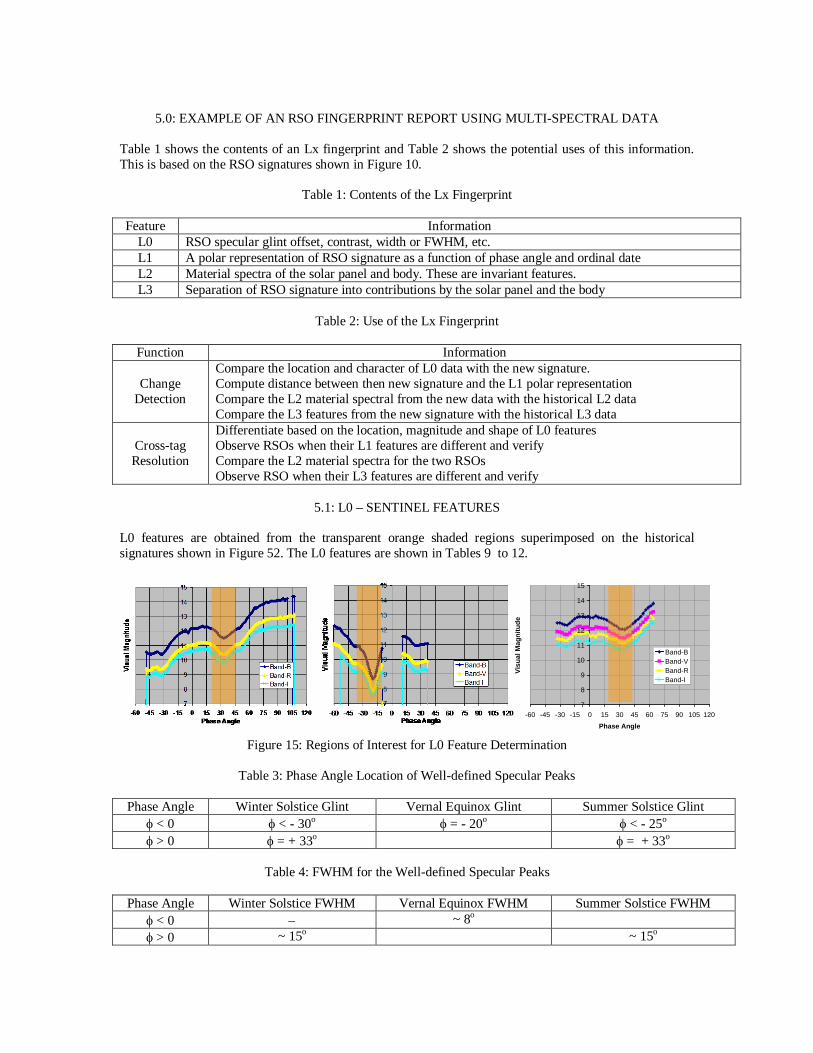
5.0: EXAMPLE OF AN RSO FINGERPRINT REPORT USING MULTI-SPECTRAL DATA

Table 1 shows the contents of an Lx fingerprint and Table 2 shows the potential uses of this information. This is based on the RSO signatures shown in Figure 10.

Table 1: Contents of the Lx Fingerprint

Feature Information L0 RSO specular glint offset, contrast, width or FWHM, etc. L1 A polar representation of RSO signature as a function of phase angle and ordinal date L2 Material spectra of the solar panel and body. These are invariant features. L3 Separation of RSO signature into contributions by the solar panel and the body

Table 2: Use of the Lx Fingerprint

Function Information

Change

Detection

Compare the location and character of L0 data with the new signature. Compute distance between then new signature and the L1 polar representation Compare the L2 material spectral from the new data with the historical L2 data Compare the L3 features from the new signature with the historical L3 data

Cross-tag Resolution

Differentiate based on the location, magnitude and shape of L0 features Observe RSOs when their L1 features are different and verify Compare the L2 material spectra for the two RSOs Observe RSO when their L3 features are different and verify

5.1: L0 – SENTINEL FEATURES

L0 features are obtained from the transparent orange shaded regions superimposed on the historical signatures shown in Figure 52. The L0 features are shown in Tables 9 to 12.

Figure 15: Regions of Interest for L0 Feature Determination

Table 3: Phase Angle Location of Well-defined Specular Peaks

Phase Angle Winter Solstice Glint Vernal Equinox Glint Summer Solstice Glint

φ < 0 φ < - 30o φ = - 20o φ < - 25o φ > 0 φ = + 33o φ = + 33o

Table 4: FWHM for the Well-defined Specular Peaks

Phase Angle Winter Solstice FWHM Vernal Equinox FWHM Summer Solstice FWHM

φ < 0 − ~ 8o φ > 0 ~ 15o ~ 15o

7

8

9

10

11

12

13

14

15

-60 -45 -30 -15 0 15 30 45 60 75 90 105 120Phase Angle

Visu

al M

agni

tude

Band-BBand-VBand-RBand-I

Table 5: Brightness of Well-defined Specular Peaks Phase Angle Winter Solstice Glint Vernal Equinox Glint Summer Solstice Glint

φ < 0 B = 10.5, R = 9.4, I = 9.0

Β = 8.7, V = 7.8, I = 7.5

B = 12.5, V = 11.7, R = 11.3, I = 10.8

φ > 0 Β = 11.5, R = 10.3, I = 9.7

Β = 12.0, V = 11.5, R = 11.0, I = 10.7

Table 6: Contrast of Well-defined Specular Peaks

Phase Angle Winter Solstice Contrast Vernal Equinox Contrast Summer Solstice Contrast

φ < 0 Β = 2.2, V = 2.0, I = 1.5

B = 0.75, V = 0.75, R = 0.75, I = 0.5

φ > 0 Β = 0.9, R = 0.9, I = 0.9

Β = 1.0, V = 0.9, R = 0.8, I = 0.5

5.2: L1 – (LIMACON PLOTS, VARIABLE FEATURES) Figure 16 shows the L1 plot for the brightness in B and R bands and the colors B-R and B-I. They were calculated using the seven steps given in Section 4.2.1. The red axis at the bottom of each figure is winter solstice and the black axis is vernal equinox. Their corresponding opposite directions would be summer solstice and autumnal equinox, respectively. Similar plots can be generated for the brightness in V and I bands and the color B-V.

Figure 16: L1 Plot for B and R Bands and the B-R and B-I colors as a function of ordinal date and the phase angle

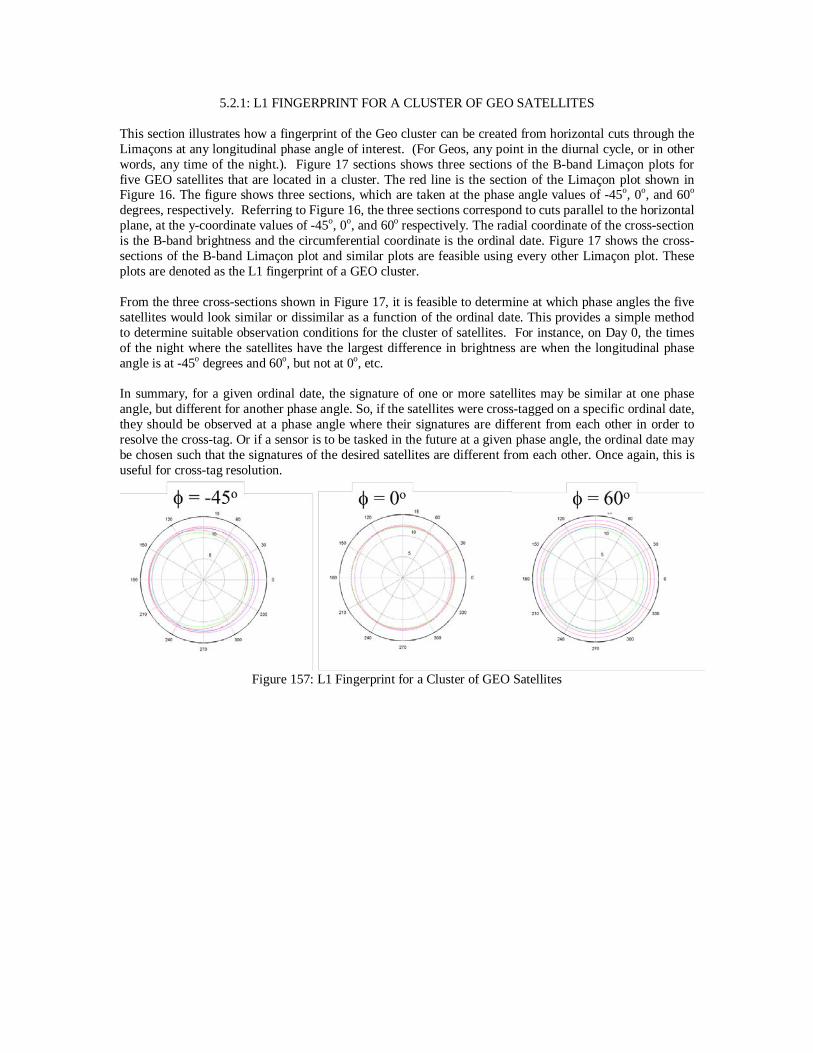
5.2.1: L1 FINGERPRINT FOR A CLUSTER OF GEO SATELLITES This section illustrates how a fingerprint of the Geo cluster can be created from horizontal cuts through the Limaçons at any longitudinal phase angle of interest. (For Geos, any point in the diurnal cycle, or in other words, any time of the night.). Figure 17 sections shows three sections of the B-band Limaçon plots for five GEO satellites that are located in a cluster. The red line is the section of the Limaçon plot shown in Figure 16. The figure shows three sections, which are taken at the phase angle values of -45o, 0o, and 60o degrees, respectively. Referring to Figure 16, the three sections correspond to cuts parallel to the horizontal plane, at the y-coordinate values of -45o, 0o, and 60o respectively. The radial coordinate of the cross-section is the B-band brightness and the circumferential coordinate is the ordinal date. Figure 17 shows the cross-sections of the B-band Limaçon plot and similar plots are feasible using every other Limaçon plot. These plots are denoted as the L1 fingerprint of a GEO cluster. From the three cross-sections shown in Figure 17, it is feasible to determine at which phase angles the five satellites would look similar or dissimilar as a function of the ordinal date. This provides a simple method to determine suitable observation conditions for the cluster of satellites. For instance, on Day 0, the times of the night where the satellites have the largest difference in brightness are when the longitudinal phase angle is at -45o degrees and 60o, but not at 0o, etc. In summary, for a given ordinal date, the signature of one or more satellites may be similar at one phase angle, but different for another phase angle. So, if the satellites were cross-tagged on a specific ordinal date, they should be observed at a phase angle where their signatures are different from each other in order to resolve the cross-tag. Or if a sensor is to be tasked in the future at a given phase angle, the ordinal date may be chosen such that the signatures of the desired satellites are different from each other. Once again, this is useful for cross-tag resolution.

Figure 157: L1 Fingerprint for a Cluster of GEO Satellites

5.3: L2 FEATURES Table 7 shows the L2 material spectra for the solar panel and the body, which are calculated by analyzing the historical signatures data. Figures 18a and d show the winter and summer solstice signatures that have been range normalized and divided by the cosine of the phase angle, cosφ (see Equations 9 and 10). These signatures are plotted against cosφ. Since cosφ is an even function, this results in the folding of the signature about the zero phase angle. The solar panel material spectrum is calculated by assuming that the body contribution remains constant in the vicinity of the specular glint (see Equations 16 and 17). This region is roughly the interval of cosφ from 0.8 to 1.0 (see Figures 18b and e). The body material spectrum is calculated by assuming that the contribution of the solar panel in the range and cosφ normalized signature is constant at large values of the phase angle (see Equation 15). This region is roughly the interval of cosφ from 0.4 to 0.6 (see Figures 18c and f). The L2 calculations are repeated for all data points in Figures 18b and e and Figure 18c and f. Figure 19a and c show the same signatures are in Figures 18a and d and the calculated results for the body spectrum from the two signatures are shown in Figures 19b and d, respectively. The solar panel spectrum is calculated from each of the two signatures are extracted using Figures 18b and e, respectively. The L2 calculation for the equinox signature is performed similarly.

Table 7: L2 Material Spectra for the Solar Panel and Body

Observation B band V band R band I band Solar Panel

Winter solstice 1.0 - ~ 0.8 ~ 0.6 Vernal equinox 1.0 - ~ 0.7 ~ 0.5 Summer solstice 1.0 ~ 0.8 ~ 0.8 ~ 0.6

Body Winter solstice 1.0 - ~ 1.0 ~ 0.8 Vernal equinox 1.0 - ~ 1.0 - Summer solstice 1.0 ~ 0.9 ~ 1.0 ~ 0.8

Figure 18: Solstice Signatures

Figure 19: Solstice Signatures and Spectra

5.4: L3 FEATURES The L3 features comprise the solar panel and body contribution to the signature. These features are extracted from the historical signatures using the L2 material spectra for the solar panel and the body given in Table 7. Figure 20 shows the individual contributions from each facet. The signature units are watt/m2 and x-axis is the phase angle. These contributions can be normalized in order to obtain the fractional abundance for the solar panel and the body in the signature as a function of time. The plot of solar panel and body contribution does not have a periodic character, which is consistent with the RSO being a three-axis stabilized object. This calculation would show a periodic character if the RSO was to become unstable.

Figure 20: Separation of Solar Panel and the Body B-band Signatures from the vernal equinox signature

6.0: EXAMPLE OF L2 FEATURES CALCULATED FROM PANCHROMATIC DATA There are two types of L2 features. First are the normalized material spectra (Section 5). The second are the contributions of the P-facet and B-facet to the signature. This is a more powerful technique because the normalized material spectra can be calculated as well from the individual contribution values if the data contains brightness information in multiple bands. In the following, an example of this technique is given for the case when the data is available only in a single band. Figure 21 shows an example of the results obtained using the method described in Section 4.3.2.4. The input data is considered to be a B-band signature data for a GEO satellite. Only four points of brightness data are used from the signature as shown in Figure 21. In other words, it is not necessary to acquire a full signature in order to use this method. It can be executed with only four points of data. Since the data happens to be available, the four point calculation was performed numerous times, each time selecting the points as defined by the mathematics. This generates results that are physically sensible for a range of ψ values from 25.8o to 43.8o. The procedure used in this calculation is described in the following: • The signature data is available as visual magnitude versus the phase angle. This data is first converted

to the flux units. The calculations cannot be performed using the logarithmic scale that is used to define the visual magnitude. (For example, smaller visual magnitude means a brighter RSO. It is counter to the sign convention in algebraic calculations.).

• Points 1, 2, 3, and 4 are selected such that the angle ψ is same at points 1 and 2, and points 3 and 4. This allows cancellation of the B-facet contribution in the visual brightness equation. The difference in the angle ψ for point 1 and 3 is approximately 100. Nine sets of such four points were selected.

0

100

200

300

400

500

600

700

-80 -60 -40 -20 0 20 40 60

Solar Panel

Body

• The contribution of P-facet and B-facet was calculated using the approach given in Section 4.3.2.4. The computed values for the P-facet and B-facet contributions are tabulated in Figure 21. The values display a monotonically increasing trend for the contribution as the phase angle reduces. For the last two points, the body contribution loses its monotonic trend. This probably means that the Taylor series linearization is too coarse an approximation.

• Figure 22 shows the contribution of the P-facet and B-facet on the signature plot itself. It shows the monotonic trend observed in the table in Figure 21. The breakdown of the signature into individual contributions of the P-facet and B-facet is an L2 feature.

Figure 161: Results for P-facet and B-facet contribution to the visual brightness

Figure 22: Display of contributions by P-facet and B-facet on the signature plot

0

20

40

60

80

100

80 -60 -40 -20 0 20 40 60 80

Body

Solar PanelGEO Signature atPhase Angle = 43o

Phase Angle

Flux

Solar PanelSignature

BodySignature

This result is a fundamental contribution to RSO fingerprinting for the following reasons: • This result is obtained from four points of single point brightness data. If the data is available in n-

bands, the P-facet and B-facet contribution can be computed in each band separately. The result is the spectral albedo-area product for the P-facet and the B-facet.

• When a RSO is functioning normally, the fractional contribution of the P-facet and B-facet will be consistent with the breakdown shown in Figure 21. If there is anomaly in the RSO, this will change.

• The calculations given in this section can be repeated for each waveband separately. This provides the spectral contribution of the P-facet and B-facet to the signature.

7.0: CONCLUSIONS AND BENEFITS OF THIS WORK

This paper presents a new framework and the accompanying algorithms for RSO fingerprinting. These algorithms are a metaphor to the techniques for human fingerprinting and they are collectively denoted as Lx techniques. The algorithms are analytical methods developed for 3-axis stabilized RSOs by using of a two-facet model. This is a reduced parameter model, which idealizes the satellite geometry as two facets. The body is represented as a single planar facet, which points to the nadir. The solar panels are also represented as a single facet, which point to the sun. The analysis assumes that the RSO geometry and surface materials are unknown but the orientation of its solar panel and body facets is known based on its orbital position and the time of observation. The algorithms are reported for the RSO fingerprint development in the visual spectrum. This characterization assumes that the primary materials of interest for an RSO are the solar panel and body materials. These materials are assumed to be unknown. If the RSO is observed at two time points when the geometric compatibility condition is fulfilled, the signature can be analytically separated into the contributions of the solar panel and the body. This calculation is performed one waveband at a time. This means that if two points of data was collected by a multi-spectral sensor when the geometry compatibility condition is satisfied, the resulting calculation provides the multi-spectral albedo-area products for the solar panel and the body. This is critical, fundamental information for the characterization of RSO surface materials. Note that this procedure derives the materials characterization based on the observation data and thus automatically accounts for space aging. This is a critical benefit because the RSO materials age significantly with the RSO time on orbit and the extent of aging varies from one RSO to another.

8.0: ACKNOWLEDGEMENT Applied Optimization, Inc. and Boeing-LTS gratefully acknowledges the support for this research by the AFRL/Space Vehicles Directorate. The work at Applied Optimization was supported by an SBIR Phase II Contract FA8718-08-C-0019.

9.0 REFERENCES 1. Jain, A., Chen, Y., and Demirkus, M., “Pores and Ridges: High-Resolution Fingerprint Matching using

Level 3 Features”, IEEE Transactions on Pattern Analysis and Machine Intelligence, Vol 29, No. 1, 2007

2. Mohsen, S.M., Zamshed Farhan, S.M., and Hashem, M.M.A., “Automated Fingerprint Recognition: Using Minutiae Matching Technique for the Large Fingerprint Database”, 3rd International Conference on Electrical and Computer Engineering, ICECE, Bangladesh, 2004

3. Tachaphetpiboon, S., and Amornraksa, T., “Fingerprint Features Extraction using Curve-Scanned DCT Coefficients”, Proceedings of Asia-Pacific Conf. on Communications, 2007

4. Chaudhary, A.B., Payne, T., Alex Quenon, “Fingerprinting of Non-resolved Three-axis Stabilized Space Objects using a Two-Facet Analytical Model”, an Air Force SBIR Phase II Final Report, AFRL-RV-HA-TR-2011-1028, 2011.

5. Chaudhary, A.B., Payne, T., Wilhelm, S., Skinner, M., Rudy, R., Russell, R., Brown. J., and Dao, P., “Analysis of Unresolved Spectral Infrared Signature for Extraction of its Invariant Features”, AMOS 2010 Technical Conference, Maui, HI 2010

6. Chaudhary, A., Payne, T., Gregory, S., and Brown, J., “RSO Fingerprinting using Non-Resolved Multi-Spectral Signatures”, SSA Meeting at AMOS 2010 Technical Conference, Maui, HI.

7. Payne, T., Chaudhary, A., Gregory, S., Brown, J., Nosek, M., “Signature Intensity Derivative and its Application to Resident Space Object Typing”, AMOS 2009 Technical Conference, Maui, HI.

8. Chaudhary, A., Payne, T., “Unresolved RSO Fingerprinting Using Time-Frequency Analysis”, Annual Report for the Phase II SBIR Project, Contract No: FA8718-08-C-0019, May 2009

9. Payne, T., and Gregory, S., “Statistical Properties of GEO Photometric Signatures”, at the AMOS Workshop on “Space Surveillance using Passive Optical Techniques for Non-resolvable Space Object Identification”, Maui, HI, 27-28 April 2006.

10. Turney, P., “The Identification of Context-Sensitive Features: A Formal Definition of Context for Concept Learning”, Proc. of the Workshop on Learning in Context Sensitive Domains, at the 13th International Conference on Machine Learning (ICML-96), Bari, Italy, 1996.

11. Limaçon, URL: www.wikipaedia.com 12. Chaudhary, A., Birkemeier, C., Gregory, S., Payne, T., and Brown, J. “Unmixing the Materials and

Mechanics Contributions in Non-resolved Object Signatures”, AMOS 2008 Technical Conference, Maui, HI

13. Kim, S., Koh, K., Lustig, M., Boyd, S., and Gorinevsky, D., "An Interior-Point Method for Large Scale l1-regularized Least Squares", IEEE Journal of Selected Topics in Signal Processing, Vol. 1, No. 4, Dec 2007

14. Candes, E., Romberg, J., "l1-magic: Recovery of Sparse Signals via Convex Programming", October 2005.

15. Huggins, P.S., Zucker, S.W., “Greedy Basis Pursuit”, Yale University, Department of Computer Science, YALEU/DCS/TR-1359, June 2006.

16. Gregory, S. and Payne, T., “GEO Signatures Database”, The Boeing Company, private communication, 2008.

17. Abbot, R.I. and Wallace, T.P., “Decision Support in Space Situational Awareness”, Lincoln Lab Journal, 2007.

18. Yedidia, J.S., Freeman, W.T., and Weiss, Y., “Understanding Belief Propagation and its Generalizations”, Mitsubishi Electric Research Laboratories, http://www.merl.com

19. Skinner, M.A., Gutierrez, D.J., Kim, D.L., Russell, R.W., Rudy, R.J., Gregory, S., Crawford, K., "Time-Resolved Infrared Spectrophotometric Observations of IRIDIUM satellites and related Resident Space Objects", IAC-09-A6.1.17, International Astronomical Congress 60th meeting, 12-16 October 2009, Daejeon, Republic of Korea.

20. Lambert, J., “Understanding the Photometric Signatures of Boeing 376 Spacecraft”, AMOS Workshop on “Space Surveillance using Passive Optical Techniques for Non-resolvable Space Object Identification”, Maui, HI, 16-17 March 2005.