HAL Id: inria-00000030https://hal.inria.fr/inria-00000030

Submitted on 16 May 2005

HAL is a multi-disciplinary open accessarchive for the deposit and dissemination of sci-entific research documents, whether they are pub-lished or not. The documents may come fromteaching and research institutions in France orabroad, or from public or private research centers.

L’archive ouverte pluridisciplinaire HAL, estdestinée au dépôt et à la diffusion de documentsscientifiques de niveau recherche, publiés ou non,émanant des établissements d’enseignement et derecherche français ou étrangers, des laboratoirespublics ou privés.

Using an Hebbian learning rule for multi-class SVMclassifiers.

Thierry Viéville, Sylvie Crahay

To cite this version:Thierry Viéville, Sylvie Crahay. Using an Hebbian learning rule for multi-class SVM classifiers..Journal of Computational Neuroscience, Springer Verlag, 2004. �inria-00000030�

Using an Hebbian learning rule for multi-class SVM

classifiers.

Thierry Vieville† and Sylvie Crahay BP 93, INRIA, Sophia, France

Abstract.Regarding biological visual classification, recent series of experiments have en-

lighten the fact that data classification can be realized in the human visual cortexwith latencies of about 100-150 ms, which, considering the visual pathways latencies,is only compatible with a very specific processing architecture, described by modelsfrom Thorpe et al.

Surprisingly enough, this experimental evidence is in coherence with algorithmsderived from the statistical learning theory. More precisely, there is a double link:on one hand, the so-called Vapnik theory offers tools to evaluate and analyze thebiological model performances and on the other hand, this model is an interestingfront-end for algorithms derived from the Vapnik theory.

The present contribution develops this idea, introducing a model derived fromthe statistical learning theory and using the biological model of Thorpe et al. We ex-periment its performances using a restrained sign language recognition experiment.

This paper intends to be read by biologist as well as statistician, as a consequencebasic material in both fields have been reviewed.

Keywords: Neuronal classifier, Supervised learning, Vapnik dimension, Biologicalmodel

† Thierry.Vieville@inria.fr, Tel: +33 6 13 28 64 59, Fax: +33 4 92 38 78 45http://www.inria.fr/Thierry.Vieville

c© 2005 Kluwer Academic Publishers. Printed in the Netherlands.

anewdraft.tex; 16/05/2005; 13:56; p.1

2

1. Introduction: biological classification is a fact

Biological visual classification1 is a well-known and very common, butstill intriguing fact. As illustrated in Fig. 1, an “object” is recognizedin very extreme situations. More generally, the ability to group stimuliinto such categories is a fundamental well-established cortical cognitiveprocess (e.g (Freedman et al., 2002)).

Figure 1. The Dalmatian in this picture (image devised by R.C. James) suddenlypops out of the senseless black blobs and dots: a small portion of bottom-up activeunits quickly lights up the whole pattern of activity (van Tonder and Ejima, 2000),even if there is no explicit visual cues (edge, texture, etc..), thus no way to explicitlyextract local features and combined for object detection (Wilson and Keil, 1999).This picture is well known because computer vision scientists confessed not beingable to analyze it (Marr, 1982) and we are not able to trace down a sequence ofsteps (if any) leading to such an holistic percept (Wilson and Keil, 1999).

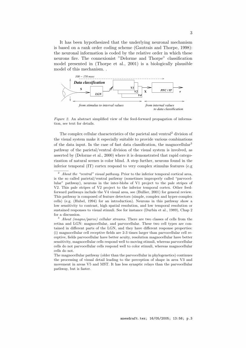
Recent series of experiments have enlighten this biological mecha-nism: data classification can be realized in the human visual cortexwith latencies of about 150 ms (Thorpe et al., 1996) and even faster(Thorpe, 2002) which, considering the visual pathways latencies (Novakand Bullier, 1997), may only be compatible with a very specific pro-cessing architecture and mechanism (Thorpe and Fabre-Thorpe, 2001).Even “high level” visual data classification such as face recognition(Delorme and Thorpe, 2001) can be realized at such a very fast rate.The feed-forward propagation of information may be summarized inFig. 2

1 In the present work, data classification simply means being able to put a uniquelabel on a given data input (e.g. “oh, there is a dog”). This differs from categorization(e.g. (Bajcsy and Solina, 1987)) where not only a label but a more complex “semanticstructure” is extracted from a given data input.

anewdraft.tex; 16/05/2005; 13:56; p.2

3

It has been hypothesized that the underlying neuronal mechanismis based on a rank order coding scheme (Gautrais and Thorpe, 1998):the neuronal information is coded by the relative order in which theseneurons fire. The connexionist ”Delorme and Thorpe” classificationmodel presented in (Thorpe et al., 2001) is a biologically plausiblemodel of this mechanism. .

LGNS

V4

V1V2 X

Data classification

from stimulus to interval values

r

100 − 150 msec

from internal values to data classification

PFC / IT

Figure 2. An abstract simplified view of the feed-forward propagation of informa-tion, see text for details.

The complex cellular characteristics of the parietal and ventral2 division ofthe visual system make it especially suitable to provide various combinationsof the data input. In the case of fast data classification, the magnocellular3

pathway of the parietal/ventral division of the visual system is involved, asasserted by (Delorme et al., 2000) where it is demonstrated that rapid catego-rization of natural scenes is color blind. A step further, neurons found in theinferior temporal (IT) cortex respond to very complex stimulus features (e.g

2 About the “ventral” visual pathway. Prior to the inferior temporal cortical area,is the so called parietal/ventral pathway (sometimes improperly called “parvocel-lular” pathway), neurons in the inter-blobs of V1 project to the pale stripes ofV2. This pale stripes of V2 project to the inferior temporal cortex. Other feed-forward pathways include the V4 visual area, see (Bullier, 2001) for general review.This pathway is composed of feature detectors (simple, complex and hyper-complexcells) (e.g. (Hubel, 1994) for an introduction). Neurons in this pathway show alow sensitivity to contrast, high spatial resolution, and low temporal resolution orsustained responses to visual stimuli. See for instance (Durbin et al., 1989), Chap 2for a discussion.

3 About (magno/parvo) cellular streams. There are two classes of cells from theretina and LGN: magnocellular, and parvocellular. These two cell types are con-tained in different parts of the LGN, and they have different response properties:(i) magnocellular cell receptive fields are 2-3 times larger than parvocellular cell re-ceptive, fields parvocellular have better acuity, resolution magnocellular have bettersensitivity, magnocellular cells respond well to moving stimuli, whereas parvocellularcells do not parvocellular cells respond well to color stimuli, whereas magnocellularcells do not.The magnocellular pathway (older than the parvocellular in phylogenetics) continuesthe processing of visual detail leading to the perception of shape in area V3 andmovement in areas V5 and MST. It has less synaptic relays than the parvocellularpathway, but is faster.

anewdraft.tex; 16/05/2005; 13:56; p.3

4

(Burnod, 1993)), regardless of size or position on the retina. For instance, someneurons in this region respond selectively to faces of particular overall featurecharacteristics. Damage in this area induce disorders4 of object recognition.There are many neuro-physiological evidences (e.g. (Durbin et al., 1989; Rollsand Treves, 1998)) about the fact that the visual temporal areas5 function isrelated to data classification.

Surprisingly enough, this experimental evidence is in coherence withalgorithms derived from the statistical learning theory, following thework of Vapnik. More precisely, there is a double link: on one hand, thestatistical learning theory offers tools to evaluate and analyze such bio-logical models and on the other hand, the Delorme and Thorpe modelis an interesting front-end for algorithms derived from the statisticallearning theory.

A step further implementations of statistical learning methods maybe efficient biologically plausible models of cortical areas involved inobject labelisation. Such an idea is for instance proposed in learningclassification in the olfactory system of insects (Huerta at al, 2004)where it is shown that neurons that perform this linear classificationare equivalent to hyperplanes tuned by local “Hebbian” learning.

The goal of this work is to develop this double link.In the next section we introduce6 the required material from statisti-

cal learning theory and consider the Guermeur multi-class SVM classi-fier, using an Hebbian learning rule to optimize the classifier. Applyingthis piece of theory, we experiment this mechanism and show that itmay be viewed as an “optimized nearest-neighbor classifier”. Thanksto these developments, we finally analyze the algorithmic and compu-tational reasons that make the Delorme and Thorpe model interestingwith respect to the statistical learning theory.

4 Common examples of such disorders include visual agnosia, or the inability toidentify objects in the visual world, and prosopagnosia, a subtype of visual agnosiathat affects specifically the recognition of once familiar faces.

5 About IT. The inferior temporal cortex is though to consist of three parts:The TEO (the occipital division of the intra-temporal cortex), the TE (the mediandivision), and the STS (superior temporal sulcus).The TEO is used for makingdiscriminations between 2-D patterns which differ in form, color, size, orientation, orbrightness. The TE is used for recognition of 3-D objects. Both the TE and STS arethought to be used in facial recognition and in the recognition of familiar objects.The STS may be the place in which the feature maps of objects (which containseparate information about each primitive of an object, such as color, orientation,or form) become object files.

6 About footnotes Since this paper presents material from both computer scienceand life science, we have introduced several footnotes reviewing basic facts for bothsizes, providing the reader with a self-contained document.

anewdraft.tex; 16/05/2005; 13:56; p.4

5

2. Implementing a multi-class SVM classifier.

Data classification with supervised deterministic learning.

In computer science, a “data classifier” provides a “label” for a datacorresponding to a set of “features” measured from inputs related tothe observed object. See (Theodoridis and Koutroumbas, 1999) for arecent comprehensive and introductory treatise on the subject.

A classifier c() is thus a function :

c : Rn → {1..R}

which associates to each data vector x ∈ Rn (data is represented by anarray of numerical values) a category r ∈ {1..R} (the class or categoryis numbered from 1 to R), with r = c(x).

Such a classifier is trained (i.e. calibrated) by a calibration set (alsocalled training set) i.e. a set of M pairs {· · · , (xi, ri), · · ·} if and onlyif ∀i, ri = c(xi). The calibration set contains typical features whichare exact data. As such, the present paradigm corresponds to super-vised learning without training error, called, say, deterministic learning.This differs7 from usual paradigms used in statistical learning, where atraining set is randomly sampled.

The fact we proposed to consider learning sets without training erroris a simple technical “simplification” to lighten the derivations. Taking“mistakes” into account is a solved problem (Vapnik, 1995; Bartlettand Shawe-Taylor, 1999; Guermeur, 2002a).

Considering a set such prototypes (either the calibration set OR animprovement of it, derived in the sequel), a natural idea is to chose thecategory of data if and only if it is “closer” to one prototype of thiscategory, than to prototypes of another category. For N prototypes,

7 Deterministic selection of calibration sample. In usual statistical approach, itis assumed that the training samples are chosen by M independent draws from thesame probability distribution as the future samples. This probability distribution isa model of the natural processes which give rise to the observed phenomenon. Thetraining samples thus provide a “view” of the underlying model.In our context, the calibration set is not “sampled” but “chosen” by an “expert”.On one hand, this means that it is a “very lucky” set of draws, without mistake. Onthe other hand, this means that the expert must randomly choose a “representative”set of draws, i.e. so that the training sample distribution correspond to the futuresamples distribution.This is not the unique strategy of such an expert: for instance a “discriminative”set of draws (in which examples close to the limit between two categories are chosenin order to help building this border, or in which “exceptional examples” are high-lighted because not easily detected otherwise) would be an interesting alternative,but in contradiction with the underlying assumptions.

anewdraft.tex; 16/05/2005; 13:56; p.5

6

the classifier is thus formally8 defined by:

c(x) = arg maxri,1≤i≤N ci(x) (1)

where ci() is the “proximity” to the ith sub-category related to theprototype xi of index i.

In the particular case where categories are linearly separable we cansimply write:

ci(x) = aTi x + bi (2)

for some ai ∈ Rn and bi ∈ R and there is a duality between suchlinear proximities and a thresholded squared distance to prototypes,as reviewed in details in appendix A. Furthermore, if we consider allcalibration data as prototypes, we obtain a classifier which outputscorrect categories for the calibration set. Frontiers between categories,are piece-wise linear, as visible in Fig. 4.

Obviously, such trivial mechanism is far from being optimal. How-ever, surprisingly enough, an optimal mechanism has a very similararchitecture, as reviewed now.

Training capability and learning performances

The Vapnik learning theory (Vapnik, 1995) allows to formalize theidea that efficient models have a limited complexity. As such, it is aformalization and in fact an improvement of the well-known Occam’sRazor principle9.

Let us review this piece of theory following recent works in thefield (Bartlett and Shawe-Taylor, 1999; Guermeur, 2002a; Guermeur,2002b). For a given classifier c in a class C of classifiers, it relates:

− the expected risk R(c) (i.e. the “average” probability for the clas-sifier to provide a wrong answer) for a set of inputs, randomlychosen according to an unknown probability distribution

8 General categories definition and prototype proximity. Let us explain why for asuitable set of function ci(), (2) defines the data category in the general case. Letus consider that each sub-category related to the prototype of index i correspondsto a “region” of the data space, defining a partition of this space. Let us definethe border of each region using, here, a general equation ci(x) = 0. This definesan hyper-surface which, according to the Jordan theorem, delimits what is inside(say when ci(x) > 0) and outside (when ci(x) < 0) this region. Here a categoryC is defined as the union of the sub-categories related to the prototype of indexi belonging to C. In this general context, equation (1) precisely determines whichci(x) > 0, thus the region of a given data. There is thus no loss of generality in thepresent approach.

9 The Ockham razor. William of Ockham (may be the most influential philoso-pher of the 14th century) stated: one should not increase, beyond what isnecessary, the number of entities required to explain anything (see for instancehttp://pespmc1.vub.ac.be/OCCAMRAZ.html for details).

anewdraft.tex; 16/05/2005; 13:56; p.6

7

with

− the empirical risk RMemp(c) (i.e. the “average” probability for the

classifier to provide a wrong answer) for the calibration set of sizeM (Here, this quantity is zero, since we have chosen to considera simple case without mistake in the calibration set and use thisfact in the derivation).

More precisely, for a chosen probability δ, the expected risk can bebounded with a probability at least 1− δ as follows:

R(c) ≤ RMemp(c) + εδ(M, C)︸ ︷︷ ︸

bias︸ ︷︷ ︸“guaranteed risk”

(3)

where the bias (also called confidence bound) εδ(M, C) is a function ofthe chosen probability δ, the calibration set size M and the “complex-ity” of the class C of classifiers, i.e. the set of classifiers used duringthe training phase.

For binary classifiers, an appropriate measure of complexity is theVapnik-Chervonenkis (VC) dimension, which -in words10- is the (even-tually unbounded) size of the largest set of points shattered withoutrestriction by the classifier functions class (Vapnik, 1998). Anothermeasure of complexity is the fat-shattering dimension,e.g. (Bartlett and Shawe-Taylor, 1999), which may be viewed as the VCdimension obtained requiring that outputs are a fixed quantity abovethe correct classification threshold.

For multi-class classifiers (Guermeur, 2002a), the covering numberNγMC at a given scale γ is a measure of complexity, and the criterionused in the sequel (Guermeur, 2002b) is based on this concept. Theauthor introduces a quantity, say the Guermeur dimension, and writtenYg here which is a monotonic function of the classifier complexity. Thisquantity is made explicit in (5).

Indeed, we expect the bias to decrease with the calibration set sizeM . The learning mechanism is consistent if and only if

limM→∞ε(M, δ, C) = 0Better than that, if the classifier functions are bounded, at the conver-gence, the smallest/optimal value of the expected risk (Vapnik, 1995) isobtained. It appears that if the classifiers class C is too large (i.e. if the

10 Intuitively, the highest this dimension, the highest the number of (eventuallyvery exotic) data set such classifier class can discriminate; with a low VC dimension,this classifier class only accepts to discriminate a restrained (expected “reasonable”or “plausible”) data set with the idea that classification is thus more robust.

anewdraft.tex; 16/05/2005; 13:56; p.7

8

complexity is too large), the process is not consistent: with a very largeclass of classifiers, we can classify everything, but what does everythingdoes anything.

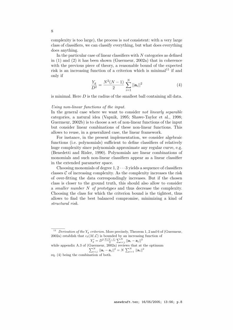
In the particular case of linear classifiers with N categories as definedin (1) and (2) it has been shown (Guermeur, 2002a) that in coherencewith the previous piece of theory, a reasonable bound of the expectedrisk is an increasing function of a criterion which is minimal11 if andonly if

Yg

D2=

N2(N − 1)2

N∑i=1

||ai||2 (4)

is minimal. Here D is the radius of the smallest ball containing all data.

Using non-linear functions of the input.In the general case where we want to consider not linearly separablecategories, a natural idea (Vapnik, 1995; Shawe-Taylor et al., 1998;Guermeur, 2002b) is to choose a set of non-linear functions of the inputbut consider linear combinations of these non-linear functions. Thisallows to reuse, in a generalized case, the linear framework.

For instance, in the present implementation, we consider algebraicfunctions (i.e. polynomials) sufficient to define classifiers of relativelyhuge complexity since polynomials approximate any regular curve, e.g.(Benedetti and Risler, 1990). Polynomials are linear combinations ofmonomials and such non-linear classifiers appear as a linear classifierin the extended parameter space.

Choosing monomials of degree 1, 2 · · · 3 yields a sequence of classifiersclasses C of increasing complexity. As the complexity increases the riskof over-fitting the data correspondingly increases. But if the chosenclass is closer to the ground truth, this should also allow to considera smaller number N of prototypes and thus decrease the complexity.Choosing the class for which the criterion bound is the tightest, thusallows to find the best balanced compromise, minimizing a kind ofstructural risk.

11 Derivation of the Yg criterion. More precisely, Theorem 1, 2 and 6 of (Guermeur,2002a) establish that εδ(M, C) is bounded by an increasing function of

Y ′g = D2 N(N−1)

2

∑N

i<j||ai − aj ||2

while appendix A.3 of (Guermeur, 2002a) reviews that at the optimum∑N

i<j||ai − aj ||2 = N

∑N

i=1||ai||2

eq. (4) being the combination of both.

anewdraft.tex; 16/05/2005; 13:56; p.8

9

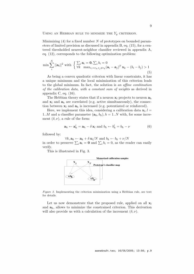
Using an Hebbian rule to minimize the Yg criterion.

Minimizing (4) for a fixed number N of prototypes on bounded param-eters of limited precision as discussed in appendix B, eq. (15), for a cen-tered thresholded nearest-neighbor classifier reviewed in appendix A,eq. (12), corresponds to the following optimization problem:

minN∑i

||ai||2 with{ ∑

i ai = 0,∑

i bi = 0∀k maxri=rk,rj 6=rk

(ai − aj)T xk − (bi − bj) > 1(5)

As being a convex quadratic criterion with linear constraints, it hasa unique minimum and the local minimization of this criterion leadsto the global minimum. In fact, the solution is an affine combinationof the calibration data, with a constant sum of weights as derived inappendix C, eq. (16).

The Hebbian theory states that if a neuron xl projects to neuron ah

and xl and ah are correlated (e.g. active simultaneously), the connec-tion between xl and ah is increased (e.g. potentiated or reinforced).

Here, we implement this idea, considering a calibration data xl, l =1..M and a classifier parameter (ah, bh), h = 1..N with, for some incre-ment (δ, ν), a rule of the form:

ah ← a′h = ah − δ xl and bh ← b′h = bh − ν (6)

followed by:∀k,ak ← ak + δ xl/N and bk ← bk + ν/N

in order to preserve∑

i ai = 0 and∑

i bi = 0, as the reader can easilyverify.

This is illustrated in Fig. 3.

a,bh a,b

X X l’l

Memorized calibration samples

Prototype’s classifier map

h’

Figure 3. Implementing the criterion minimization using a Hebbian rule, see textfor details.

Let us now demonstrate that the proposed rule, applied on all xl

and ah, allows to minimize the constrained criterion. This derivationwill also provide us with a calculation of the increment (δ, ν).

anewdraft.tex; 16/05/2005; 13:56; p.9

10

Let us thus look for a (δ, ν) increment decreasing the constrained criterion(5).Writing δ = 2κ (xT

l ah)/||xl||2, and assuming xl 6= 0 (otherwise theHebbian rule has no effect) and xT

l ah 6= 0 (otherwise our derivation issingular), the criterion decreases if and only if:

||a′h||2 = δ2 ||xl||2 − 2 δ (xTl ah) + ||ah||2 ≤ ||ah||2

⇔ 4 κ2 (xTl ah)2/||xl||2 − 4 κ(xT

l ah)2/||xl||2 ≤ 0⇔ κ2 − κ ≤ 0⇔ 0 ≤ κ ≤ 1

the decrease being maximal for κ = 1/2, while the decrease for valuesκ > 1/2 corresponds to a decrease for a value 1− κ, below 1/2.

We thus look for a couple (κ, ν), 0 ≤ κ ≤ 1/2, with a maximal valueof κ while the constraints:

maxri=rk[aT

i xk − bi]−maxrj 6=rk[aT

j xk − bj ] > 1are verified.

These constraints can be rewritten in a more compact form:

if rk = rh max (u′k, wk − ck κ + ν) > vk

if rk 6= rh uk > max (v′k, wk − ck κ + ν) (7)

with the following notations:u′k = maxri=rk,i 6=h[aT

i xk − bi] vk = maxrj 6=rk[aT

j xk − bj ] + 1uk = maxri=rk

[aTi xk − bi]− 1 v′k = maxrj 6=rk,j 6=h[aT

j xk − bj ]wk = aT

h xk − bh ck = 2 (xTl ah) (xT

l xk)/||xl||2(8)

A step further, since these constraints were already verified at theprevious step, for the previous value of (ah, bh) i.e. for κ = ν = 0 we alsocan write, from (7):

if rk = rh then max(u′k, wk) > vk and if rk 6= rh then uk > max(v′k, wk)As a consequence, (i) if rk = rh and u′k > vk, the corresponding inequalityis already verified and (ii) if rk 6= rh we already have uk > v′k.

The inequalities (7) thus reduce to:

if rk = rh and u′k ≤ vk wk − ck κ + ν > vk

if rk 6= rh uk > wk − ck κ + ν

finally rewritten as:

maxrk=rh,u′k≤vk

(vk − wk + ck κ) < ν < minrk 6=rh(uk − wk + ck κ)

Summarizing: in order to find a solution to (6) decreasing (5), wehave to look for a maximal value of κ compatible with the followinginequalities (written using (8)):

0 ≤ κ ≤ 1/2νmin(κ) < νmax(κ) with

{νmin(κ) = maxrk=rh,u′

k≤vk

(vk − wk + ck κ)νmax(κ) = minrk 6=rh

(uk − wk + ck κ)(9)

anewdraft.tex; 16/05/2005; 13:56; p.10

11

while κ = 0 is a known solution.Let us finally note12 that the same method could have been used to

minimize the Guermeur criterion11 Y ′g instead of Yg.

Convergence of the mechanismIf there is an increment (δ, ν) for which the criterion decreases whilepreserving the constraints, the rule is repeated. Otherwise, this meansthat there is no linear combination of the form ah+ =

∑k δhk xk which

decreases this convex criterion. Because of convexity, there is thus nolocal linear variation, which improves this criterion. We thus are at alocal minimum, this local minimum being the solution of the convexproblem.

Furthermore, we may choose ah and xl either sequentially (as in ourcomputer implementation, where we select the couple which inducesa maximal local decrease of the criterion), in parallel or randomly, assoon as all couples are finally selected, the choice of a strategy beingof no influence on the final result, but only the calculation duration.

Edition of the set of prototypesModifying (ah, bh) corresponds to a modification of the related proto-type xh = Λ−1 (cah + a)/2 as made explicit in appendix A. We thusoptimize the related set of prototypes of this nearest-neighbor classifier.This differs from the choice of support vectors in a SVM.

Furthermore, in (9), if ∀k, rk = rh, u′k > vk there is no minimalbound for ν, thus no maximal bound for bh in (6). As a consequence bh

may have huge values, large enough for the hth not to be used anymorein the comparison process. This simply means that this prototype isredundant and can thus be deleted. This mechanism thus automaticallyedit the corresponding prototype list.

However, when N varies, the criterion (5) is not necessarily convexas a function of N and only a local minimum is targeted.

12 Using Hebbian rules to minimize the Y ′g dimension. If we consider the mini-

mization of∑N

i<j||ai − aj ||2 instead of

∑N

i||ai||2 in (5) using the Hebbian rule

defined in (6) we easily derive:

arg minah

∑N

i<j||ai − aj ||2 = arg minah

∑N

j 6=h||ah − aj ||2

so that if we replace ah with a′h = ah − δ xl in order to obtain:∑N

j 6=h||ah − aj ||2 ≥

∑N

j 6=h||a′h − aj ||2

=∑N

j 6=h||ah − aj ||2 − 2 δ

∑N

j 6=h(ah − aj)

T xl + δ2∑N

j 6=h||xl||2

writing δ = 2 κ∑N

j 6=h(ah − aj)

T xl/∑N

j 6=h1/||xl||2 the previous inequality reduces

to 0 ≤ κ ≤ 1 as for the derivation proposed for Yg and the rest of the derivation isidentical, as the reader can easily verify.

anewdraft.tex; 16/05/2005; 13:56; p.11

12

Implementation detailsAs far as, a computer implementation is to be derived, the linear pro-gramming problem in (9) can be solved, searching a maximal valueκ ∈ [0..1/2] such that νmin(κ) < νmax(κ) using a dichotomy methodand choosing:

δ = 2κ (xTl ah)/||xl||2 and, say, ν = (νmin(κ) + νmax(κ))/2

Adaptivity of the mechanismAs soon as a calibration data (xk, rk) is added to the calibration set,without any lack of reactivity, the system is able to provide a first-approximation classification, inserting this data as a new prototypean applying the trivial nearest-neighbor classification mechanism, asreviewed in appendix A.

This not an optimal solution and the minimization of (5) takesplace, but is an independent process, realized “when time is available”.

As soon as a calibration data is deleted, the current solution is simplyto be re-optimized, taking benefit of the fact that one constraint isremoved.

With, these simple rules, the learning mechanism is entirely adap-tive with respect to calibration data addition / deletion and also withrespect to the computation time resources.

Biological plausibilityThis mechanism corresponds to a so-called Hebbian-like learning rulesas extensively discussed elsewhere(Durbin et al., 1989; Rolls and Treves, 1998; Gisiger et al., 2000).

As far as biological plausibility is concerned, the previous derivationstates that any a small κ > 0 compatible with (9) decreases the crite-rion. A biological system may thus simply use “epsilon-values”, (say,κ ' 10−3 since all quantities have been normalized with respect tounity), checking νmin(κ) < νmax(κ) in (9).

The whole mechanism thus reduces to (1) linear operations (ad-dition or scalar multiplication) which biological plausibility has beenextensively discussed, e.g. (Bugmann, 1997), (2) a min/max operatoralso biologically plausible as reviewed in e.g. (Yu et al., 2003) and (3)“switches” (detecting redundant data, detecting if an increment is valid,etc..) which is related to so-called inhibition mechanisms, commonlyobserved in such biological neuronal layers, e.g. (Gisiger et al., 2000).

Considering the architecture of this mechanism we merge a sim-ple nearest-neighbor classifier which may be implemented as standardneuronal network, e.g. (Theodoridis and Koutroumbas, 1999) with aHebbian learning rule. This rule simply derives from a statistical learn-ing criterion, contrary to e.g. (Soo-Young and Dong-Gyu, 1996) where

anewdraft.tex; 16/05/2005; 13:56; p.12

13

the theoretical justification of the generalization performances is onlybased on a heuristic.

Implementations of SVM like classifiers using fast and simple learn-ing mechanisms has been introduced as “kernel adaptron” methods(Friess et al, 1998) but without a true Hebbian rule as here. Similarly(Krauth and Mezard, 1987) proposed the so called “monivar” learningalgorithms in neural networks maximizing the geometrical margin andused in feed-forward layered networks (Mezard and Nadal, 1989) underthe name of “tiling” algorithm.

3. Experimental results

Interactive 2D demonstration

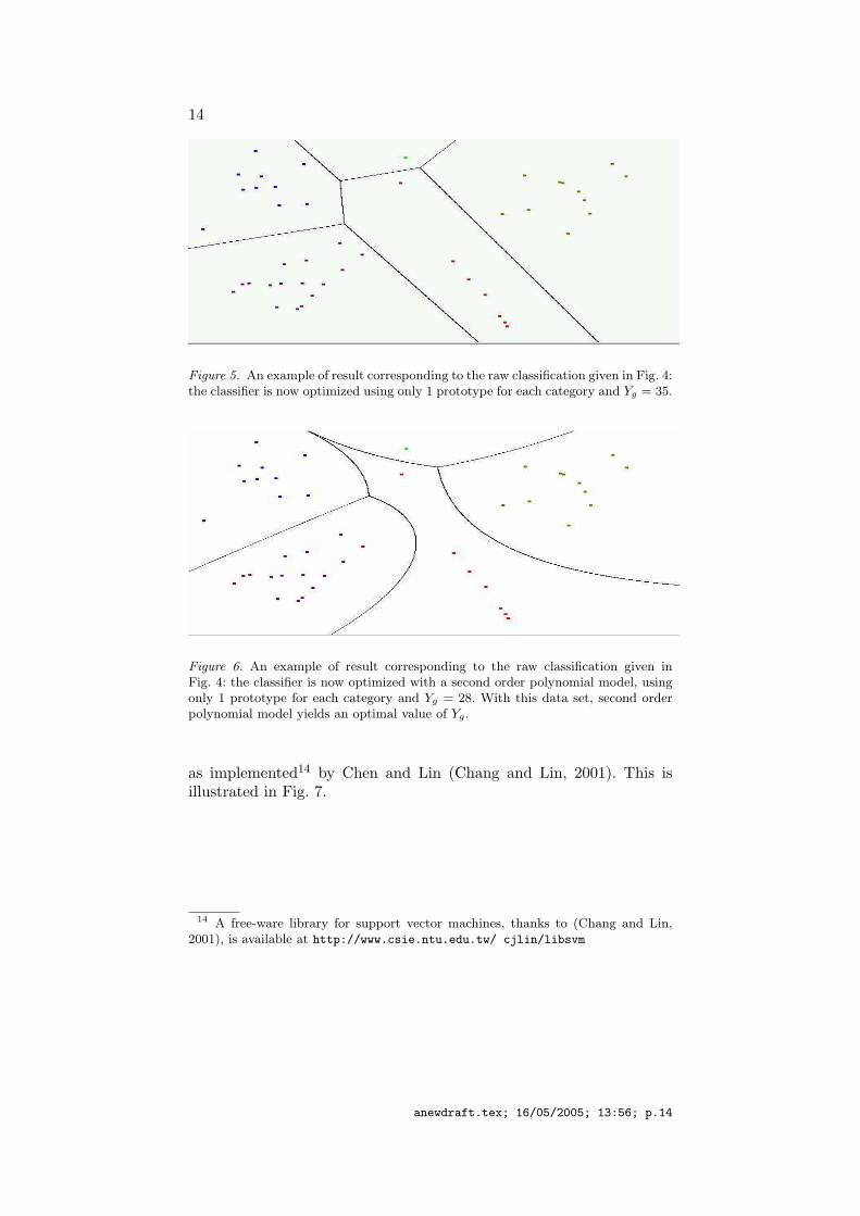
Please refer to the on-line13 software documentation for details aboutthe software module. Examples of results, shown in Fig.5 and 6, illus-trate the method behavior and allow to validate the implementation.The module can be experimented on Internet.

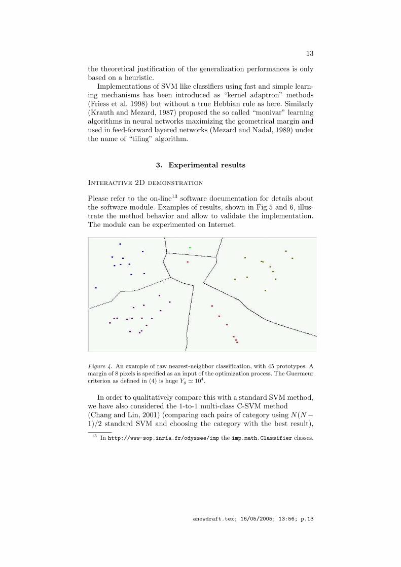
Figure 4. An example of raw nearest-neighbor classification, with 45 prototypes. Amargin of 8 pixels is specified as an input of the optimization process. The Guermeurcriterion as defined in (4) is huge Yg ' 104.

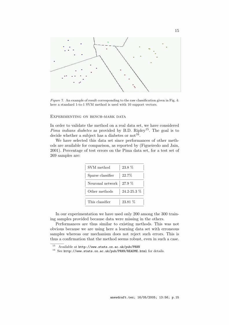
In order to qualitatively compare this with a standard SVM method,we have also considered the 1-to-1 multi-class C-SVM method(Chang and Lin, 2001) (comparing each pairs of category using N(N−1)/2 standard SVM and choosing the category with the best result),

13 In http://www-sop.inria.fr/odyssee/imp the imp.math.Classifier classes.

anewdraft.tex; 16/05/2005; 13:56; p.13

14

Figure 5. An example of result corresponding to the raw classification given in Fig. 4:the classifier is now optimized using only 1 prototype for each category and Yg = 35.

Figure 6. An example of result corresponding to the raw classification given inFig. 4: the classifier is now optimized with a second order polynomial model, usingonly 1 prototype for each category and Yg = 28. With this data set, second orderpolynomial model yields an optimal value of Yg.

as implemented14 by Chen and Lin (Chang and Lin, 2001). This isillustrated in Fig. 7.

14 A free-ware library for support vector machines, thanks to (Chang and Lin,2001), is available at http://www.csie.ntu.edu.tw/ cjlin/libsvm

anewdraft.tex; 16/05/2005; 13:56; p.14

15

Figure 7. An example of result corresponding to the raw classification given in Fig. 4:here a standard 1-to-1 SVM method is used with 10 support vectors.

Experimenting on bench-mark data

In order to validate the method on a real data set, we have consideredPima indians diabetes as provided by B.D. Ripley15. The goal is todecide whether a subject has a diabetes or not16.

We have selected this data set since performances of other meth-ods are available for comparison, as reported by (Figueiredo and Jain,2001). Percentage of test errors on the Pima data set, for a test set of269 samples are:

SVM method 23.8 %

Sparse classifier 22.7%

Neuronal network 27.9 %

Other methods 24.2-25.3 %

This classifier 23.81 %

In our experimentation we have used only 200 among the 300 train-ing samples provided because data were missing in the others.

Performances are thus similar to existing methods. This was notobvious because we are using here a learning data set with erroneoussamples whereas our mechanism does not reject such errors. This isthus a confirmation that the method seems robust, even in such a case.

15 Available at http://www.stats.ox.ac.uk/pub/PRNN16 See http://www.stats.ox.ac.uk/pub/PRNN/README.html for details.

anewdraft.tex; 16/05/2005; 13:56; p.15

16

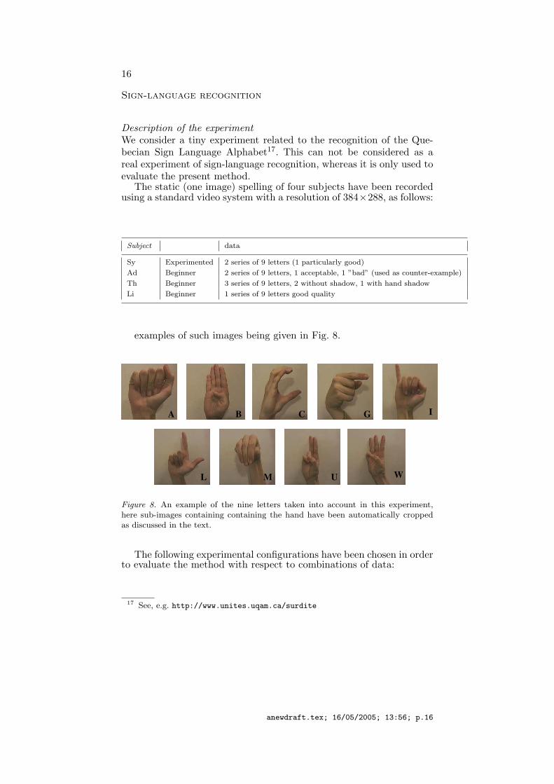
Sign-language recognition

Description of the experimentWe consider a tiny experiment related to the recognition of the Que-becian Sign Language Alphabet17. This can not be considered as areal experiment of sign-language recognition, whereas it is only used toevaluate the present method.

The static (one image) spelling of four subjects have been recordedusing a standard video system with a resolution of 384×288, as follows:

Subject data

Sy Experimented 2 series of 9 letters (1 particularly good)

Ad Beginner 2 series of 9 letters, 1 acceptable, 1 ”bad” (used as counter-example)

Th Beginner 3 series of 9 letters, 2 without shadow, 1 with hand shadow

Li Beginner 1 series of 9 letters good quality

examples of such images being given in Fig. 8.

A

W

B C G I

L M U

Figure 8. An example of the nine letters taken into account in this experiment,here sub-images containing containing the hand have been automatically croppedas discussed in the text.

The following experimental configurations have been chosen in orderto evaluate the method with respect to combinations of data:

17 See, e.g. http://www.unites.uqam.ca/surdite

anewdraft.tex; 16/05/2005; 13:56; p.16

17

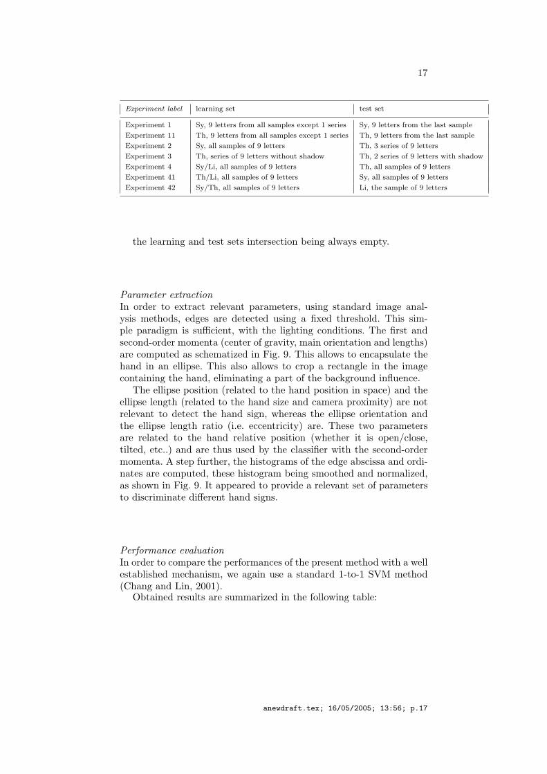
Experiment label learning set test set

Experiment 1 Sy, 9 letters from all samples except 1 series Sy, 9 letters from the last sample

Experiment 11 Th, 9 letters from all samples except 1 series Th, 9 letters from the last sample

Experiment 2 Sy, all samples of 9 letters Th, 3 series of 9 letters

Experiment 3 Th, series of 9 letters without shadow Th, 2 series of 9 letters with shadow

Experiment 4 Sy/Li, all samples of 9 letters Th, all samples of 9 letters

Experiment 41 Th/Li, all samples of 9 letters Sy, all samples of 9 letters

Experiment 42 Sy/Th, all samples of 9 letters Li, the sample of 9 letters

the learning and test sets intersection being always empty.

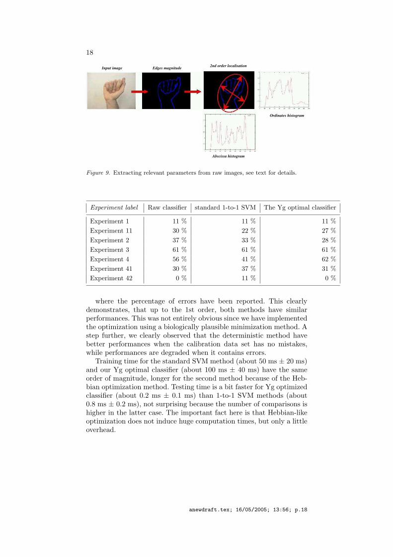
Parameter extractionIn order to extract relevant parameters, using standard image anal-ysis methods, edges are detected using a fixed threshold. This sim-ple paradigm is sufficient, with the lighting conditions. The first andsecond-order momenta (center of gravity, main orientation and lengths)are computed as schematized in Fig. 9. This allows to encapsulate thehand in an ellipse. This also allows to crop a rectangle in the imagecontaining the hand, eliminating a part of the background influence.

The ellipse position (related to the hand position in space) and theellipse length (related to the hand size and camera proximity) are notrelevant to detect the hand sign, whereas the ellipse orientation andthe ellipse length ratio (i.e. eccentricity) are. These two parametersare related to the hand relative position (whether it is open/close,tilted, etc..) and are thus used by the classifier with the second-ordermomenta. A step further, the histograms of the edge abscissa and ordi-nates are computed, these histogram being smoothed and normalized,as shown in Fig. 9. It appeared to provide a relevant set of parametersto discriminate different hand signs.

Performance evaluationIn order to compare the performances of the present method with a wellestablished mechanism, we again use a standard 1-to-1 SVM method(Chang and Lin, 2001).

Obtained results are summarized in the following table:

anewdraft.tex; 16/05/2005; 13:56; p.17

18

Input image Edges magnitude 2nd order localisation

Ordinates histogram

Abscissa histogram

Figure 9. Extracting relevant parameters from raw images, see text for details.

Experiment label Raw classifier standard 1-to-1 SVM The Yg optimal classifier

Experiment 1 11 % 11 % 11 %Experiment 11 30 % 22 % 27 %Experiment 2 37 % 33 % 28 %Experiment 3 61 % 61 % 61 %Experiment 4 56 % 41 % 62 %Experiment 41 30 % 37 % 31 %Experiment 42 0 % 11 % 0 %

where the percentage of errors have been reported. This clearlydemonstrates, that up to the 1st order, both methods have similarperformances. This was not entirely obvious since we have implementedthe optimization using a biologically plausible minimization method. Astep further, we clearly observed that the deterministic method havebetter performances when the calibration data set has no mistakes,while performances are degraded when it contains errors.

Training time for the standard SVM method (about 50 ms ± 20 ms)and our Yg optimal classifier (about 100 ms ± 40 ms) have the sameorder of magnitude, longer for the second method because of the Heb-bian optimization method. Testing time is a bit faster for Yg optimizedclassifier (about 0.2 ms ± 0.1 ms) than 1-to-1 SVM methods (about0.8 ms ± 0.2 ms), not surprising because the number of comparisons ishigher in the latter case. The important fact here is that Hebbian-likeoptimization does not induce huge computation times, but only a littleoverhead.

anewdraft.tex; 16/05/2005; 13:56; p.18

19

4. Discussion

Evaluation of the Delorme and Thorpe model performancesRegarding fast data classification, the Delorme and Thorpe model(Thorpe et al., 2001) is based on the fact that very short observedlatencies are only compatible with an information flow related to theoccurrence of a neuronal signal than to e.g. the spike frequency. Further-more, since the latency of a given neuron is a direct decreasing functionof the neuron input value, only neurons with the highest values generatespikes fast enough to be taken into account. This has two consequences.

Quantification of the neuronal information: the quantitativevalue of the signal is directly related to the spike delay and is thus abounded value with a finite precision. Let us consider that the temporaldiscrimination of a neuron, see e.g. (Carr, 1993) for an extensive study,is of about τ = 1 ms, so that two spikes arriving within the samemillisecond are viewed as simultaneous. Since neural inputs receivedduring a temporal window of T = 10..20 ms (Thorpe et al., 2001) istaken into account, the temporal resolution18 is σ = T/τ . Consideringother coding scheme, such as phase coding(Gutierrez-Galvez and Gutierrez-Osuna, 2003), a similar analysis ofbounded values with a finite precision is derivable.

Sparseness of the neuronal information: among the rather hugenumber of input neurons (typically the dimension n of the neuronal“vector” has an order of magnitude of 105) only a rather small number(' 103) is taken into account. Here we consider that this selection ismade during the learning phase, for a given set of prototypes. This dif-fers from thresholding the highest values, which is a non-linear process.As mentioned by one of the reviewer of this paper, a strict analysisshould also consider the effects of allowing a choice of 103 non-zeroparameters from among the 105 possibles, leading to an additionalincrease of the classification complexity.

In the computer implementation of the Delorme and Thorpe model(called spike-net, e.g. (Delorme et al., 1999)) a “nearest-neighbor” mech-

18 About rate-coding combinations. If we consider the rate coding scheme (Thorpeet al., 2001), there seems to be N ! possible permutations for a given set of N data.However, in practice, at a given temporal resolution τ and during a time windowT it is not possible to observe all these permutations. If at a given time t, aninput i has been detected, all inputs in the It = [t..t + τ ] interval are viewed as“synchronous with i”. Such It interval is not fixed but triggered by the 1st occurringinput. However, we are in a situation where N is very large, so that at the end ofeach It interval yet another spike very likely (almost) immediately occurs, startinga new It+τ interval and finally allowing to consider consecutive intervals of durationτ , like when building a temporal “histogram” of the spike occurrences. The numberof possible combination is thus of o(σN ).

anewdraft.tex; 16/05/2005; 13:56; p.19

20

anism behavior is implemented with an underlying “semi-distance”based on such finite precision quantification and sparse representation.This corresponds to the present framework and we can take a lookat its complexity, without detailing the algorithm. In the particularcase where this classifier is used as a binary classifier we can easilyquantify its complexity, using the V C dimension (Vapnik, 1998) whichis bounded 19 by:

V C ≤ min

([D2

ρ2

], n

)+ 1 (10)

Here, with the assumptions of appendix B, from (14), D2/ρ2 = σ2/4 '102 (this being an order of magnitude) leading to a small V C dimension,which does neither depend on the number of neuronal units nor on thecomplexity of the front-end mechanisms of extraction of data features.This is clearly not the case for standard neuronal networks used asclassifiers, because considering for instance their V C dimension again,it is higher than the order of magnitude of the number of neurons. Moreprecisely (Baum and Haussler, 1989), for an arbitrary feed-forwardneuronal network with a binary activation function the Vc dimensionis of o(W log(W )) where W is the number of weights free parametersin the network, while (Koiran and Sontag, 1996) for a multi-layer feed-forward neuronal network with a sigmoid activation function, the Vc

dimension is of o(W 2).Considering the biological model (Thorpe et al., 2001) we can con-

jecture that, similarly, the neuronal model has a bounded complexity,not because of the sparseness of the neuronal information but becauseof its quantification. A precise analysis is perspective of the presentwork.

ConclusionThe present approach allows to re-interpret basic nearest-neighbor clas-sifiers, using the statistical learning theory, obtaining an optimizedversion of this basic mechanism. A key feature is that optimizing thestatistical property of nearest-neighbor classifiers allows to automati-cally add/delete prototypes, edit them and remove redundant ones.

We also have made explicit and experimented that SVM like mech-anisms can easily be implemented using Hebbian-like correction rules.Such optimization mechanism is not as fast as the standard method,but its biological plausibility is better, while final performances aresimilar.

19 The smallest integer higher than[D2/ρ2

]is considered in this formula.

anewdraft.tex; 16/05/2005; 13:56; p.20

21

This point of view is in deep relation with fast visual recognition inthe brain. It may, for instance, explain why biological classifiers havesuch surprising generalization performances.

More precisely, the Thorpe et al. model complexity is bounded anddoes not depends on the network size. It is likely bounded because ofthe quantification steps (in relation with the temporal resolution ofneuronal encoding). This explains its very good performances.

References

Bajcsy, R. and F. Solina: 1987, ‘Three Dimensional Object Representation Revis-ited’. In: Proceedings of the 1st International Conference on Computer Vision.London, England, IEEE Computer Society Press.

Bartlett, P. and J. Shawe-Taylor: 1999, ‘Generalization Performance of SupportVector Machines and Other Pattern Classifiers’. In: B. Scholkopf, C. Burges,and A. Smola (eds.): Advances in Kernel Methods, Support Vector Learning.The MIT Press, Cambridge, Chapt. 4, pp. 43–54.

Baum, E. and D. Haussler: 1989, ‘What size net gives valid generalization’. NeuralComputation 1, 151–160.

Benedetti, R. and J.-J. Risler: 1990, Real algebraic and semi-algebraic sets. Hermann,Paris.

Bugmann, G.: 1997, ‘Biologically plausible neural computation’. Biosystems 40,11–19.

Bullier, J.: 2001, ‘Integrated model of visual processing’. Brain Res. Reviews 36,96–107.

Burnod, Y.: 1993, An adaptive neural network: the cerebral cortex. Masson, Paris.2nd edition.

Carr, C. E.: 1993, ‘Processing of Temporal Information in the Brain’. Annu. Rev.Neurosci. 16, 223–244.

Chang, C.-C. and C.-J. Lin: 2001, ‘Training nu-Support Vector Classifiers: Theoryand Algorithms’. Neural Computation 13(9), 2119–214.

Cover, T. and P. Hart: 1967, ‘Nearest Neighbor Pattern Classification’. IEEETrans.on Information Theory 13(1).

Delorme, A., J. Gautrais, R. VanRullen, and S. J. Thorpe: 1999, ‘SpikeNET: A simu-lator for modeling large networks of integrate and fire neurons’. Neurocomputing26, 989–996.

Delorme, A., G. Richard, and M.Fabre-Thorpe: 2000, ‘Rapid Categorisation of nat-ural scenes is colour blind: A study in monkeys and humans’. Vision Research40(16), 2187–2200.

Delorme, A. and S. Thorpe: 2001, ‘Face processing using one spike per neuron:resistance to image degradation.’. Neural Networks 14, 795–804.

Duda, R. O., P. E. Hart, and D. G. Stork: 2000, Pattern Classification, 2nd edition.Wiley Interscience.

Durbin, R., C. Miall, and G. Mitchinson (eds.): 1989, The computing neuron.Addison-Wesley.

Figueiredo, M. A. T. and A. K. Jain: 2001, ‘Bayesian Learning of Sparse Classifiers’.In: Computer Vision and Pattern Recognition.

anewdraft.tex; 16/05/2005; 13:56; p.21

22

Freedman, D. J., M. Riesenhuber, T. Poggio, and E. K. Miller: 2002, ‘CategoricalRepresentation of Visual Stimuli in the Primate Prefrontal Cortex’. Science291(5502), 312–316.

T. Friess, N. Cristianini, and C. Campbell. The kernel adatron algorithm: a fast andsimple learning procedure for support vector machine. In Proc. 15th InternationalConference on Machine Learning. Morgan Kaufman, 1998.

Gaspard, F. and T. Vieville: 2000, ‘Non Linear Minimization and Visual Localiza-tion of a Plane’. In: The 6th International Conference on Information Systems,Analysis and Synthesis, Vol. VIII. pp. 366–371.

Gautrais, J. and S. Thorpe: 1998, ‘Rate Coding vs Temporal Order Coding : atheorical approach’. Biosystems 48, 57–65.

Gisiger, T., S. Dehaene, and J. P. Changeux: 2000, ‘Computational models ofassociation cortex’. Curr. Opin. Neurobiol. 10, 250–259.

Guermeur, Y.: 2002a, ‘Combining discriminant models with new multi-class SVMs’.Pattern Analysis and Applications 5(2), 168–179.

Guermeur, Y.: 2002b, ‘A simple unifying theory of Multi-Class Support VectorMachines’. Technical Report 4669, INRIA.

Gutierrez-Galvez, A. and R. Gutierrez-Osuna: 2003, ‘Pattern completion throughphase coding in population neurodynamics’. Neural Networks 16, 649–656.

Hubel, D.: 1994, L’oeil, le cerveau et la vision : les etapes cerebrales du traitementvisuel, L’univers des sciences. Pour la science.

R. Huerta, T. Nowotn, M. Garcıa-Sanchez, H. D. I. Abarbanel, and M. I. Rabinovich.Learning classification in the olfactory system of insects. in preparation, 2004.

Koiran, P. and E. Sontag: 1996, ‘Neural Networks with quadratic VC dimension’.Advances in Neural Information Processing System 8, 197–203.

W. Krauth and M. Mezard. Learning algorithms with optimal stability in neuralnetworks. J. Phis., 20:745–752, 1987.

Marr, D.: 1982, Vision. W.H. Freeman and Co.M. Mezard and J. Nadal. Learning in feed forward layered networks: The tiling

algorithm. Journal of Physics, 22:2191–2204, 1989.Novak, L. and J. Bullier: 1997, The Timing of Information Transfer in the Visual

System, Vol. 12 of Cerebral Cortex, Chapt. 5, pp. 205–241. Plenum Press, NewYork.

Rolls, E. T. and A. Treves: 1998, Neural networks and brain function. Oxforduniversity press.

Shawe-Taylor, J., P. Bartlett, R. Williamson, and M. Anthony: 1998, ‘Structuralrisk minimization over data-dependent hierarchies’. IEEE Trans. on InformationTheory 44(5).

Soo-Young, L. and J. Dong-Gyu: 1996, ‘Merging Back-propagation and HebbianLearning Rules for Robust Classifications’. Neural Networks 9(7), 1213–1222.

Theodoridis, S. and K. Koutroumbas: 1999, Pattern Recognition. Academic Press.Thorpe, S.: 2002, ‘Ultra-Rapid Scene Categorization with a Wave of Spikes’. In:

Biologically Motivated Computer Vision, Vol. 2525 of Lecture Notes in ComputerScience. pp. 1–15, Springer-Verlag Heidelberg.

Thorpe, S., A. Delorme, and R. VanRullen: 2001, ‘Spike based strategies for rapidprocessing.’. Neural Networks 14, 715–726.

Thorpe, S. and M. Fabre-Thorpe: 2001, ‘Seeking categories in the brain’. Science291, 260–263.

Thorpe, S., D. Fize, and C. Marlot: 1996, ‘Speed of processing in the human visualsystem’. Nature 381, 520–522.

anewdraft.tex; 16/05/2005; 13:56; p.22

23

van Tonder, G. J. and Y. Ejima: 2000, ‘Bottom - up clues in target finding: Why aDalmatian may be mistaken for an elephant’. Perception 29(2), 149 –157.

Vapnik, V.: 1995, The Nature of Statistical Learning Theory. Springer-Verlag.Vapnik, V.: 1998, Statistical Learning Theory. John Wiley.Vieville, T.: 2000, ‘Using markers to compensate displacements in MRI volume

sequences.’. Technical Report 4054, INRIA.Vieville, T., D. Lingrand, and F. Gaspard: 2001, ‘Implementing a multi-model

estimation method’. The International Journal of Computer Vision 44(1).Wilson, R. and F. Keil: 1999, The MIT Encyclopedia of the Cognitive Sciences. MIT

Press, Cambridge, MA.Yu, A. J., M. Giese, and T. Poggio: 2003, ‘Biophysiologically plausible implementa-

tions of maximum operation’. Neural Computation 14(12).

Acknowledgments: Arnaud Delorme, Simon Thorpe and Yann Guermeur are grate-

fully acknowledged for some powerful ideas in this work.

We are especially thankful for the deep help of the reviewers during the reviewing process.

Appendix

A. Thresholded nearest-neighbor (NN) classifiers.

Linear classifiers correspond to thresholded NN classifiers.Within the generic framework proposed in (1), for any metric ||v||2Λ =vT Λv of Rn, defined by a positive definite symmetric matrix Λ, letus consider for some thresholds θi, the following so called centeredthresholded linear squared proximity to a prototype, i.e. :

ci(x) =[−||x− xi||2Λ + θi +

(||x||2Λ − aT x + b

)]/c

= aTi x− bi with

{ai = [2Λxi − a] /cbi =

[||xi||2Λ − θi − b

]/c

(11)

choosinga = 2Λ

∑Nj=1 xj/N , b =

∑Nj=1[||xj ||2Λ − θj ]/N and c = 4n

whilexi = Λ−1 (cai + a)/2 and θi = ||cai + a||2Λ−1/4− (c bi + b)

so that each proximity is parameterized by ai and bi. Here we:

1. consider the opposite of the squared distance ||x − xi||2Λ, say theproximity, to the prototype xi for the chosen metric,

2. thresholded by θi in order to :- control the relative influence of each prototype (the higher θi thehigher the proximity to the ith prototype) and also to :- obtain a one to one correspondence between the linear functionparameters (ai, bi) and the prototype data and threshold (xi, θi) upto an indetermination parameterized by (a, b, c),

anewdraft.tex; 16/05/2005; 13:56; p.23

24

3. add the same quantity ||x||2Λ − aT x + b to each ci(x) and multiplyby a common positive constant c so that:- the comparison in (1) is not modified, while:- adding ||x||2Λ allows to cancel quadratic terms in (11) and obtaina linear function and- indetermination20 in the definition of (ai, bi) is canceled, verifyingthe constraints:

N∑i=1

ai = 0 andN∑

i=1

bi = 0 (12)

so that (ai, bi) are centered while∑N

i=1 ||ai||2 is minimal21 w.r.t. a.

As a consequence we obtain a linear classifier and frontiers Fij be-tween categories of index i and j are piece-wise planar hyper-surfacesof equation:

Fij = {x, ci(x)− cj(x) = [ai − aj ]T x + [bi − bj ] = 0}as illustrated in Fig. 4. The distance from a prototype to the categoryfrontier (geometrical margin) writes:

d(xi, Fij) = 1/2 [||xi − xj ||Λ + [θi − θj ]/||xi − xj ||Λ]as easily derived22 since c ||ai − aj ||Λ−1 = 2 ||xi − xj ||Λ.

Properties and limitations of NN classifiers.In the statistical interpretation of NN classifiers (e.g.(Theodoridis and Koutroumbas, 1999)), under “reasonable” assump-tions, i.e. normal distribution of the data in each category with similarcovariances, this corresponds to a Bayesian classifier, writing

θi = 2 log(p(ri)) < 0 where p(ri) = eθi/2/∑

j eθj/2

20 Invariance in the arg-max equation: In equation (1), the reader can easily verifythat any strictly increasing transformation t : R → R of the proximities ci(x), i.e.ci(x) → t(ci(x)) will not change the comparisons. On the reverse, if t() is not astrictly increasing transformation comparisons may be modified for some ci(x).The most general transformation is thus a composition with a strictly increasingfunction.Now, if we want to preserve the linearity, i.e. that ci(x) being linear, t(ci(x)) isstill linear, this transformation must be linear, the only solution being of the formt(ci(x)) = [ci(x)− (aT x− b)]/c with c > 0.We also observe that this classifier with N (n + 1) components has (N − 1) (n +1) − 1 independent parameter components, i.e. degrees of freedom, because n + 2parameters are constrained via the choice of a, b and c.

21 If we consider the criterion mina||a′i||2 with a′i = ai − a the related normal

equation is precisely∑N

i=1a′i = 0.

22 Distance to an hyper-plane. The distance d(x, P ) is the minimal value ||x−z||Λfor a point z ∈ P , i.e. with aT z− b = 0. Writing this as a criterion:

minz maxλ12||x− z||2Λ + λ (aT z− b)

the normal linear equations yield the formula: d(x, P ) = |aT x− b|/||a||Λ−1

anewdraft.tex; 16/05/2005; 13:56; p.24

25

is the a-priori probability for a given data to belong the ith sub-category.

Beside being conceptually extremely simple and also obvious toimplement in practice, this well-known classifier (Duda et al., 2000)has reasonable performances. More precisely, the probability of errorfor the nearest neighbor rule (i.e. with θi = 0 in (11)) given enoughmembers in the training set is sufficiently close to the Bayes (optimal)probability of error. It has been shown (Cover and Hart, 1967) thatas the size of the training set goes to infinity, the asymptotic nearestneighbor error is never two times worse than the Bayes (optimal) error.However, calibration or training set sizes never go to infinity! The realproblem is to understand the performances of the classifier for a limitedcalibration set, as discussed in this paper.

Furthermore, the present approach does not provide, as it, any“modelization” of the calibration set. As a consequence, since no predic-tion/inference is possible with this method, the quality of the trainingis highly dependent upon the calibration set itself. It may not be very“accurate” with respect to data which are not calibration data, i.e.generalization performances are expected to be poor (Vapnik, 1995).

Another traditional criticism about NN classifiers pointed at largespace requirement to store the entire calibration set and the seem-ing necessity to query the entire calibration set in order to make asingle membership classification. There has been considerable inter-est in editing the training or calibration set in order to reduce itssize (e.g.: proximity graphs, Delaunay triangulation) eliminating “re-dundant” data (see (Duda et al., 2000) for a review). Such editingmechanisms only delete redundant prototypes, whereas a much generalmechanism is proposed here.

B. Considering bounded parameters of limited precision.

As noticed, e.g. in (Gaspard and Vieville, 2000), at the specificationlevel, a “physical” parameter is always represented though a vector ofbounded quantities, xi, xi

min ≤ xi ≤ ximax with a finite precision xi

ε sothat there is a finite range of significant values. This finite range size isσi =

[(xi

max − ximin)/xi

ε

]. This specification also applies, up to the 1st

order, to non-linear combinations23 of parameters.23 The bound and 1st order precision of a monomial. We also consider non-linear

combinations of parameters, using rescaled monomial mα = [∏n

i=1(xi)αi ]/m of

degrees α = (· · · , αi, · · ·) bounded by |mα| ≤ σα, with:σα = 1/

∑n

j=1αj/(σj/2)αj and m =

∏n

i=1(σi/2)αi/σα

easily derived because on one hand, since |xi| ≤ σi/2 it is straightforward to derive

anewdraft.tex; 16/05/2005; 13:56; p.25

26

Using the transformation xi → xi/xiε−ci with ci = (xi

max+ximin)/(2 xi

ε)from now on and without any loss of generality we can consider xi

ε = 1and that the quantity is bounded24 by |xi| ≤ σi/2: quantities are nowcentered and rescaled with respect to their precision.

Such a precision is in practice very easy to estimate (e.g. 1 mm fora pupil ruler, 1 deg for a protractor, 1 pixel in an image, etc...) andso are bounds. These quantities are not precise numbers but orders ofmagnitude.

Following this track, two parameters xi and x′i can be considereddistinct only if25:|xi − x′i| > 2Otherwise, we cannot decide whether (i) these values are the same or(ii) differ by a quantity too small to be measurable. In the latter case,we can not say that they are equal, but indistinguishable.

A step further, a vectorial centered rescaled parameters are boundedby26

||x||∞ ≤ maxiσi/2 and ||x|| ≤ D =

√∑i

(σi)2/2 (13)

e.g. if all sizes σi = σ are equal D =√

n σ/2.Two vectorial parameters are indeed distinguishable if at least one

component is distinguishable: |xi−x′i| > 2 for some i (i.e. ||x−x′||∞ >2). But what happens if we combine quantities which are “almost dis-tinguishable” ? The data space dimension being in practice very large,we interpret the precision uncertainty27 as an additive Gaussian noiseso that, if x and x′ correspond to the same quantities, ||x−x′||2 followsa Ξ-square distribution which expected value is n, so that ||x−x′||/

√n

|mα| ≤ σα =∏n

i=1(σi/2)αi/m.

On the other hand, considering that precision is a 1st order quantity, since:∂mα ' 1/m

∑n

j=1αj

∏n

i=1,i6=j(xi)αi (xj)αj−1 ∂xj

writing xjε = |∂xj | = 1 we obtain

mαε ≤ 1/m

∑n

j=1αj

∏n

i=1(σi/2)αi/(σj/2)αj = 1

which is in fact the tightest bound not dependent on xi.24 Here, xi

min ≤ xi ≤ ximax ⇔ |xi − (xi

max + ximin)/2| ≤ (xi

max − ximin)/2 yields

|xi/xiε − ci| ≤ σi/2 with our notations.

25 Here, we have to double the value of the bound because each value may varyin a ±1 range thus their difference may vary in twice this range.

26 Here, we write ||x||∞ = maxi|xi| and ||x||2 =∑

i(xi)2, derivation of (13) being

obvious.27 Interpreting bounded precision as uncertainty: we assume that if xi an x′i are two

samples of the same quantity, εi = xi−x′i is a normalized centered Gaussian variableof variance 1, so that |xi − x′i| < 2 with a probability P > 0.95. If |xi − x′i| > 2 wethus can consider that xi an x′i likely correspond to different quantities.In the vectorial case ||x − x′||2 =

∑i(εi)2 follows a Ξ-square distribution with n

degrees of freedom, thus of mean n and variance 2 n.

anewdraft.tex; 16/05/2005; 13:56; p.26

27

is expected to be 1. In coherence to the 1D case, we distinguish twoquantities when the value is twice the expected value.

Summarizing, we propose to consider the average quadratic preci-sion28, specifying that two vectorial are distinguishable if and only if||x− x′||/

√n > 2.

From these specifications we introduce a natural but importantconstraint for our paradigm: data from the learning set must be distin-guishable, i.e. two learning data xi and xj must verify ||xi−x

′i|| > 2√

n,the so-called geometrical margin e.g. (Vapnik, 1998) being ρ =

√n. If

two prototypes belonging to different categories are indistinguishable,the corresponding categories are indistinguishable and the problemill-posed: this situation is to be rejected. A useful relation is

D/ρ = 1/2√∑

i

(σi)2/n (14)

with D/ρ = σ/2 if all sizes σi = σ are equal.Furthermore, in (1), comparisons of the form ci(x) > cj(x) between

two proximities are valid if and only if their difference is higher thatthe related precision. For thresholded nearest-neighbor proximities asdefined in (11), ci(x) = [−||x−xi||2+· · ·]/c so that, from what precedes,we must write

ci(x) > cj(x) + γ with γ = [2√

n]2/c = 1 (15)

Over-simple, such an specification is very useful at both the theo-retical and implementation29 levels.

28 About the metric related to data precision. Here quantities are rescaled beforecomputing Euclidean distances, i.e. it writes

||xi − x′i|| =

√∑n

i=1

[xi−x

′i

xiε

]2This diagonal metric has an obvious statistical interpretation in terms of the inverseof a covariance or “quadratic information’, e.g. (Vieville et al., 2001), interpretingthe data precision as an uncertainty. The precision between two components mayalso be “coupled” (i.e. correlated), the metric not being diagonal anymore. It is how-ever obvious to diagonalize any covariance matrix, considering linear combinationsof these components and obtain decoupled components. There is thus no lack ofgenerality with the present “diagonal” approach.

29 Physical parameter specification and local estimation. It has been observed (e.g.(Vieville, 2000)) that there is a real gain to take this experimental specification intoaccount: with such specification, “quasi-static” estimation methods, with step bystep variations from an initial estimate towards the problem solution, are powerfulstrategies for local estimations (adaptations to limited range variations from a de-fault value, interactive estimation where a user given initial estimate is to be refined,efficiency in tracking tasks ...), experimentally more efficient than standard usual

anewdraft.tex; 16/05/2005; 13:56; p.27

28

C. Deriving the form of the Y g minimum

In order to solve the minimization problem in (5), we can easily writethe Lagrangian of this constrained criterion:

L =12

N∑i

||ai||2+∑i j k

αijk

[(ai − aj)T xk − (bi − bj)− 1

]+α

∑i

bi+βT∑

i

ai

with the related Kuhn-Tucker30 conditions:

αijk > 0⇔

ri = arg maxri=rk

aTi xk + bi

and rj = arg maxrj 6=rkaT

j xk + bj

and (ai − aj)T xk − (bi − bj) = 1

and the related normal equations:{0 = ∂L

∂bh=∑

i k αihk −∑

j k αhjk + α =∑

k αhk + α

0 = ∂L∂ah

T= ah +

∑j k αhjk xk −

∑i k αihk xk + β = ah −

∑k αhk xk + β

with αhk =∑

i αihk −∑

j αhjk.The optimal solution of (5) thus writes:

ah =∑k

αhk xk − β with∑k

αhk + α = 0 (16)

methods, because the stability of the estimation process is easy to control in thiscase. Furthermore, the estimation is stopped as soon as the required precision isobtained, whereas for standard methods, convergence to a non-negligible precisiononly is not so easy to obtain, so that overhead occurs. This mechanism is used inour implementation.

30 On Kuhn-Tucker conditions. We consider for the purpose of this derivation,weak inequalities (≥) instead of strict inequalities (>). The Kuhn-Tucker conditionsstate that the Lagrangian multiplier αijk (i) vanishes if and only if the inequalityis strictly verified and (ii) is positive if the inequality is verified as an equality. Inpractice, this bound is numerically never attained.

anewdraft.tex; 16/05/2005; 13:56; p.28