using autodock for virtual...

1

Using AutoDock for Virtual Screening

Written by William Lindstrom, Garrett M. Morris,

Christoph Weber and Ruth Huey

The Scripps Research Institute Molecular Graphics Laboratory

10550 N. Torrey Pines Rd. La Jolla, California 92037-1000

USA

3 August 2006, v7

2

Contents

Contents.............................................................................................................. 2

Introduction ........................................................................................................ 4 Before We Start…........................................................................................... 4

FAQ – Frequently Asked Questions .............................................................. 7

Exercise One: Populating the Ligand Directory: sdf to pdb .................... 9 NCI Diversity Set............................................................................................. 9 Babel................................................................................................................ 9 Documentation ................................................................................................ 9 Procedure: ..................................................................................................... 10

Exercise Two: Processing the ligands: pdb to pdbq. ............................. 12 Procedure: ..................................................................................................... 12

Exercise Three: Profiling the library: determining the covering set of Atom Types: ..................................................................................................... 14

Procedure: ..................................................................................................... 14

Exercise Four: Preparing the receptor: pdb to pdbqs. ............................ 16 Procedure: ..................................................................................................... 16

Exercise Five: Preparing AutoGrid Parameter Files for the library ....... 18 Procedure: ..................................................................................................... 18

Exercise Six: Calculating atomic affinity maps for a ligand library using AutoGrid............................................................................................................ 20

Procedure: ..................................................................................................... 20

Exercise Seven: Validating the Protocol with a Positive Control .......... 22 Procedure: ..................................................................................................... 22

Exercise Eight: Preparing the Docking Directories and Parameter Files for each ligand in a library............................................................................. 24

Procedure: ..................................................................................................... 24

Exercise Nine: Launching many AutoDock jobs....................................... 26 Procedure: ..................................................................................................... 26

Exercise Ten: Identifying the Interesting Results to Analyze................. 28 Procedure: ..................................................................................................... 28

Exercise Eleven: Examine Top Dockings.................................................. 30

Using the TSRI cluster: bluefish................................................................... 32

3

Files for exercises: ......................................................................................... 34 Input Files: ..................................................................................................... 34 Results Files .................................................................................................. 34

Ligand........................................................................................................ 34 Macromolecule ......................................................................................... 34 AutoGrid .................................................................................................... 34 AutoDock................................................................................................... 34

Appendix A: Usage for AutoDockTools Scripts ........................................ 35

4

Introduction

This tutorial will introduce you to the process of virtual screening using UNIX shell commands and python scripts in the AutoDock suite of programs. There are nine steps in the tutorial in which we will prepare a library of ligand files and corresponding AutoGrid and AutoDock parameter files for the library, use AutoGrid to calculate maps, launch AutoDock calculations for each ligand (see Figure 1.1 below) followed by two analysis steps in which we will extract and evaluate the results (Exercises 10 and 11, not shown). In addition we will focus on the data structures and documentation necessary for large scale calculations.

Before We Start…

We’ll use the directory /usr/tmp for the tutorial today. In practice you’ll use a directory of your own choosing.

Open a Terminal window and then type this at the UNIX, Mac OS X or Linux prompt:

Figure 1.1 VS Tutorial Map

System requirements: this tutorial requires that you have cvs and either babel or OpenBabel on your computer as well as AutoDockTools.

5

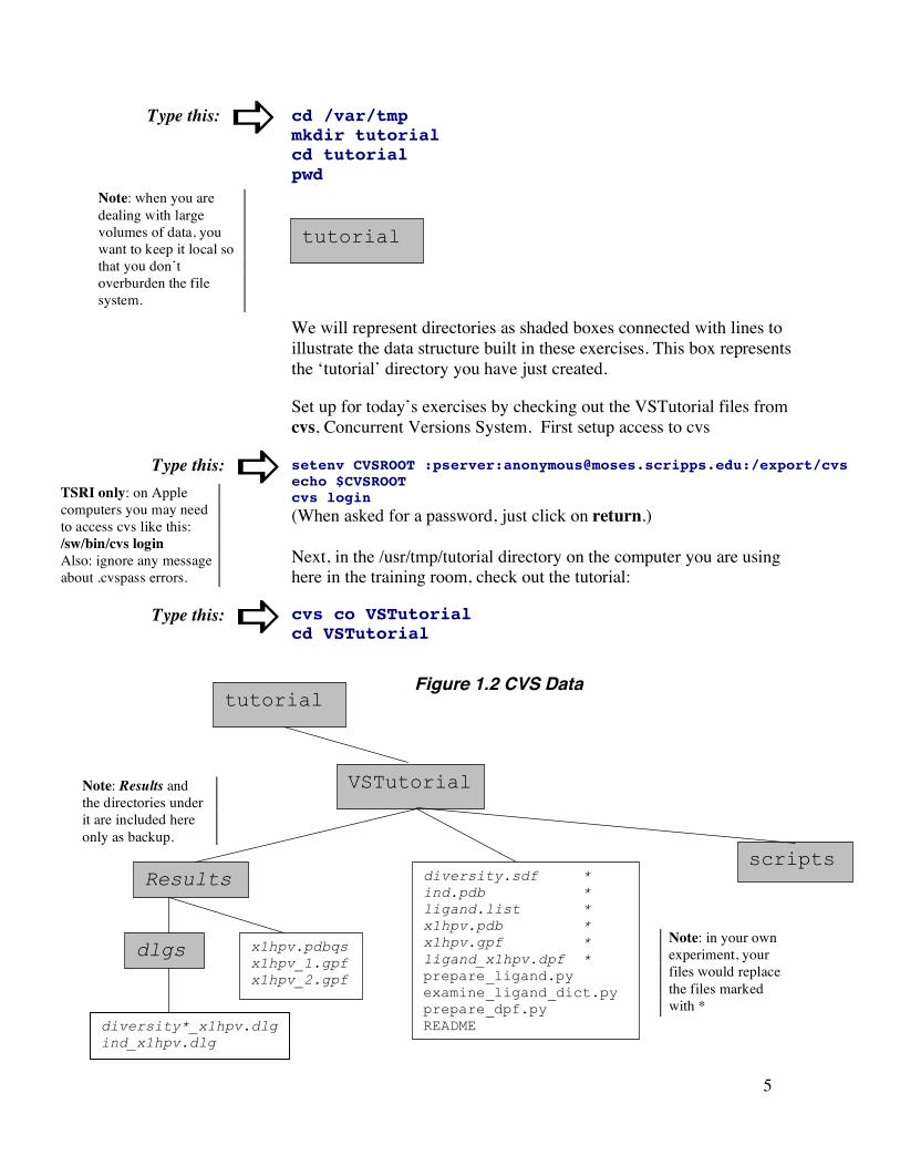
cd /var/tmp mkdir tutorial cd tutorial pwd

We will represent directories as shaded boxes connected with lines to illustrate the data structure built in these exercises. This box represents the ‘tutorial’ directory you have just created.

Set up for today’s exercises by checking out the VSTutorial files from cvs, Concurrent Versions System. First setup access to cvs setenv CVSROOT :pserver:[email protected]:/export/cvs echo $CVSROOT cvs login (When asked for a password, just click on return.) Next, in the /usr/tmp/tutorial directory on the computer you are using here in the training room, check out the tutorial:

cvs co VSTutorial cd VSTutorial

tutorial

Type this:

Note: when you are dealing with large volumes of data, you want to keep it local so that you don’t overburden the file system.

Type this:

Type this:

tutorial

VSTutorial

Results scripts

diversity.sdf * ind.pdb * ligand.list * x1hpv.pdb * x1hpv.gpf * ligand_x1hpv.dpf * prepare_ligand.py examine_ligand_dict.py prepare_dpf.py README

dlgs x1hpv.pdbqs x1hpv_1.gpf x1hpv_2.gpf

diversity*_x1hpv.dlg ind_x1hpv.dlg

Note: in your own experiment, your files would replace the files marked with *

Note: Results and the directories under it are included here only as backup.

Figure 1.2 CVS Data

TSRI only: on Apple computers you may need to access cvs like this: /sw/bin/cvs login Also: ignore any message about .cvspass errors.

6

#!/bin/csh # # $Id: ex00.csh,v 1.3 2005/01/31 18:11:28 lindy Exp $ # # Because this script uses "pwd" to set VSTROOT it matters # where (which directory you run it from. This script # should be run as "source ./scripts/ex00.csh" So, # after you did your "cvs co VSTutorial" a "VSTutorial" # directory was created and that's the one that should be # your working directory when you source this script. # # set up the root directory of the Virtual Screening # Tutorial # setenv VSTROOT `pwd`

$VSTROOT: a short cut to the directory in which your Virtual Screening Tutorial activities will take place.

tutorial

VSTutorial

$VSTROOT

Results scripts

Type this: source scripts/ex00.csh

echo $VSTROOT

Figure 1.3 $VSTROOT

Note: here we use the backward-slanted single quotation mark. UNIX replaces strings enclosed by this character by the result of executing them. Here `pwd` is replaced by ‘/usr/tmp/tutorial/VSTutorial’before setenv is executed.

You must setup your environment to access to babel, python, adt, autodock3 and autogrid3. For TSRI users: source scripts/setpath.csh (others need to edit the script for their local file systems)

Type this:

Note: you will need to source these two scripts in any new terminal you open during this tutorial to properly set up the environment in that new terminal.

7

FAQ – Frequently Asked Questions

1. What library should I use for screening? If you want to try and find novel compounds, you probably want to use a library designed for diversity, one which probes a large ‘chemical space.’ If there are small molecules which are known to bind to your macromolecule, you may want to construct a tailored library of related compounds.

2. How much computational time should be invested in each compound? How many dockings, how many evaluations? It depends on your receptor and on the computational resources available to you. One recent successful AutoDock Virtual Screening used 100 dockings with 5,000,000 evaluations per docking per compound.

3. How do I know which docking results are ‘hits’?

When the results are sorted by lowest-energy, the compounds which bind as well as your positive control or better can be considered potential hits. (Remember to allow for the ~2.1 kcal/mol standard error of AutoDock). If you have no positive control, consider the compounds with the lowest energies as potential hits.

4. What’s the best way to analyze the results?

Sort them by lowest energy first, then use ADT to inspect the quality of the binding.

5. Will I need to visualize the results with the best energies? Generally it is wise to inspect the top 30 to 50 results. Some people advocate visually inspecting the top 100-400 hits.

6. What should I look for when I visualize a docked compound? The first thing to check is that the ligand is docking into some kind of pocket on the receptor. The second is that there is a chemical match between the atoms in the ligand and those in the receptor. For example, check that carbon atoms in the

8

ligand are near hydrophobic atoms in the receptor while nitrogens and oxygens in the ligand are near similar atoms in the binding pocket. Check for charge complementarity. Check whatever else you may know about your particular system: for instance, if you know that the enzymatic action of your protein involves a particular residue, examine how the ligand binds to that residue. In the case of HIV protease, good inhibitors bind in a mode which mimics the transition state.

7. Where can I get help?

The AutoDock mailing list is a good place to start. Information about it and other AutoDock resources can be found on the AutoDock Web site:

http://www.scripps.edu/mb/olson/doc/autodock

9

Exercise One: Populating the Ligand Directory: sdf to pdb

The library used for a virtual screening experiment is a selected group of ligand files. Sources of libraries include Maybridge (www.maybridge.com), MDL Mentor, Available Chemicals (UW-Madison), NCI among many others. Libraries are characterized according to their uniqueness, diversity and drug-likeness which is based on Lipinsky’s “Rule of Five” which consists of four criteria: molecular weight <500, logP <5, number of hydrogen bond donors<5 and number of hydrogen bond acceptors < 10.

The size of the library which can be screened depends on the available computational resources. Typically libraries number in the tens to hundreds of thousands of files. It is practically impossible to test exhaustively any large chemical database. Libraries are constructed to maximize the chances of obtaining good ‘hits’ by focusing on ligand diversity.

NCI Diversity Set To expedite drug discovery, the National Cancer Institute maintains a resource of more than 140,000 synthetic chemicals and 80,000 natural products for which it can provide samples for high-through-put screening (HTS). The NCI Diversity Set is a collection of 1990 compounds selected to represent the structural diversity in the whole resource.

Babel The standard file format for ligand libraries in the pharmaceutical industry is sdf (MDL Isis). The Open Source program babel is a program for converting various types of data files to other formats. To see a list of supported types, you can type babel –m which starts babel in the ‘menu’ mode. Type Control-C to exit the menu mode. The first exercise illustrates the use of babel to convert information from an sdf file into 100 pdb files which can be read by scripts available in AutoDockTools.

Documentation Documenting each step of a computational experiment in sufficient detail to be able to reproduce it is an essential requirement. README files are one common form of documentation. Important sections in a README file for computation experiments include:

10

Project, Author, Date, Task, Data sources, Files in this directory, Output files, Running Scripts and other notes on the location of the executable and environmental settings.

In the “Before We Start…” section, you set up local copies of the input files and executable scripts we will use today.

Procedure:

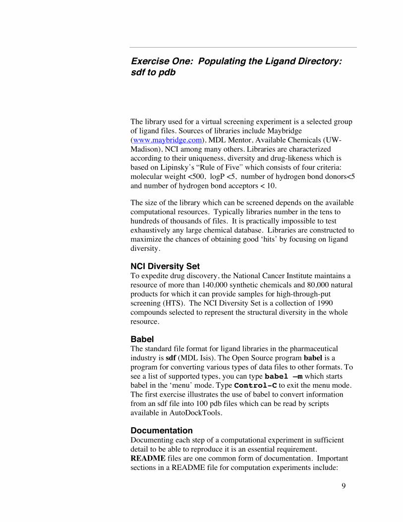
1. In ex01.csh, we create a working directory called VirtualScreening and two subdirectories: one called Ligands where we will do all the preparation of the ligand files and a second called etc where we’ll keep a few extra, useful files. Next we use babel to extract and convert to pdb format the ~100 files specified by index in ligand.list. These files are extracted from diversity.sdf, an sdf file containing the NCI Diversity Set. Finally, we add a positive control, ind.pdb, to the list of ligands.

#!/bin/csh # $Id: ex01.csh,v 1.3 2005/01/31 01:28:12 lindy Exp $ # Create the directory in which all your Virtual # Screening Tutorial activities will take place: cd $VSTROOT mkdir VirtualScreening # Create the Ligands and etc subdirectories: cd VirtualScreening mkdir Ligands mkdir etc # Copy the list of ligands to the etc directory: cp ../ligand.list etc #make the Ligands directory the current working directory cd Ligands # Convert the .sdf file to a collection of pdb files: foreach f (`cat ../etc/ligand.list`) echo $f babel -isdf ../../diversity.sdf "$f"-"$f" –opdb \ diversity"$f".pdb # for OpenBabel-1.100.2 # babel -isdf ../../diversity.sdf -f "$f" -l "$f" –opdb \ #diversity"$f".pdb end # Copy ind.pdb down from the tutorial files into Ligands: cp ../../ind.pdb .

Note: We use ligand.list to specify which files to extract from the sdf library file. These were chosen to give a distribution of docked energies vs our protein, hsg1

Note: This script uses babel, the syntax for which varies between versions. Type “which babel” to find out your version. Then edit this script to fit your version if necessary. Also: we use this tortured babel syntax in order to preserve the original compound numbers which can be used to request samples from NCI.

Note: here we use foreach to execute each line up to end on every item returned by result of cat … which is the list of ligands.

11

source $VSTROOT/scripts/ex01.csh

2. Let’s look at the list we used foreach f (`cat ../etc/ligand.list`) echo $f end 3. To confirm that the foreach loop and babel did what we expected, list the pdb files. Use wc (word count) for counting. Check that the number of pdb files 108 matches the number of ligands in the ligand.list file 107 plus one for ind.pdb, the positive control which we added: \ls *.pdb \ls *.pdb | wc -l wc -l ../etc/ligand.list 4. Document the experiment: cd $VSTROOT vim README

Fill in Project, Author, Date, Data sources, Files in this directory and an entry for this section’s procedure.

tutorial

VSTutorial

$VSTROOT

VirtualScreening Results scripts

etc Ligands

Type this:

diversity*.pdb ind.pdb

ligand.list

Type this:

Figure 1.4 Exercise 1 Result

Type this:

12

Exercise Two: Processing the ligands: pdb to pdbq.

An AutoDock experiment results in docked ligand structures which represent the best (lowest energy) conformation found in the specified search space. Input molecule files for an AutoDock experiment must conform to the set of atom types supported by AutoDock. This set consists of united-atom aliphatic carbons, aromatic carbons in cycles, polar hydrogens, hydrogen-bonding nitrogens and directionally hydrogen-bonding oxygens among others, each with a partial charge.

Properly prepared molecule input files for AutoDock consist of pdb-like records for each atom, conforming to this AutoDock atom type set. Thus file preparation must include fixing a number of potential problems such as missing atoms, added waters, more than one molecule, chain breaks, alternate locations etc.

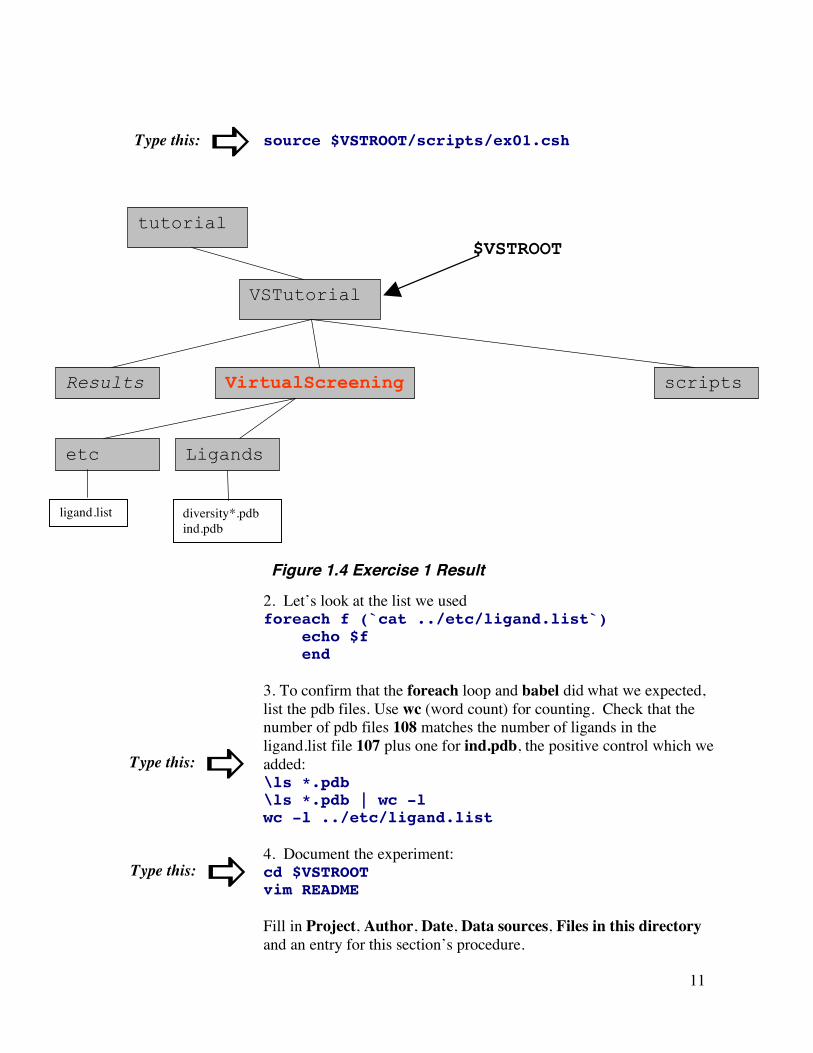
In the tutorial, UsingAutoDockwithAutoDockTools, you prepared the ligand file using ADT, a graphical user interface. It is not reasonable to try to prepare thousands of ligand files using a graphical user interface. Tasks of this magnitude must be automated. In this exercise we introduce prepare_ligand.py, a python script in the AutoDockTools module, and how to use it in a Unix foreach loop. Details of its usage can be found in the Appendix.

Procedure:


#!/bin/csh # $Id: ex02.csh,v 1.2 2005/01/31 00:48:01 lindy Exp$ # # use the prepare_ligands.py script to create pdbq files cd $VSTROOT/VirtualScreening/Ligands foreach f (`ls *.pdb`) echo $f ../../prepare_ligand.py -l $f -o "$f"q –d \ ../etc/ligand_dict.py end

Type this:

Note: The prepare_ligand.py script takes as input a pdb or mol2 file (specified on the command line with the -l switch) and writes a pdbq file with charges, root, and rotatable bonds defined. The -d switch specifies the filename of a python dictionary that describes the atomtypes and other attributes of the set of input files processed. This information will be used in the next exercise.

13

2. Examine the results of this script:

\ls *.pdbq |wc \ls ../etc

3. Document: Add an entry for this section’s procedure to the README file. Record warning messages. Here 10 input files raised the warning “Not all ligand written:” The UNIX ‘script filename’ command is an alternative to the README file convention. It copies all the text from the terminal into the specified transcript file. Here, you could start a transcript before the foreach loop. To stop recording the transcript file, type Control D.

tutorial

VSTutorial

$VSTROOT


etc Ligands

diversity*.pdbq ind.pdbq

ligand_dict.py

Figure 1.5 Exercise 2 Result Note: ligand_dict.py is generated by prepare_ligand.py and used in Exercise 3.

Type this:

14

Exercise Three: Profiling the library: determining the covering set of Atom Types:

In docking a ligand against a receptor, AutoDock uses a special representation of the receptor: a set of grid-based potential energies files called 'grid maps'. AutoGrid is used to precalculate one grid map for each atom type present in the ligand to be docked. A grid map consists of a three dimensional lattice of regularly spaced points, surrounding the receptor (either entirely or partly) and centered on some region of interest of the macromolecule under study. Each point within the grid map is the sum of the pairwise potential interaction energy of a probe atom of a particular type with each of the atoms in the macromolecule. The 3-dimensional volume covered by the grid maps in conjunction with the 'n' active torsions in the ligand defines the 6 + 'n' dimensioned search space.

In docking a set of ligands against a single receptor, you need only one grid map for each atom type in the covering set of atom types present in the ligands. In this exercise we write a summary of the ligand library in order to determine the covering set of atom types and to exclude ligands with too many atoms, atom types, rotatable bonds, etc

Procedure:

Notice the covering set of atoms. You may decide to remove some stems based on this information.


Note: AutoDock limits the number of atoms in the ligand to 4096, the number of different atom types in a ligand to 6 and the number of rotatable bonds in a ligand to 32. This will change..

#!/bin/csh # $Id: ex03.csh,v 1.4 2005/01/31 02:23:44 lindy Exp $ # The examine_ligand_dict.py scripts reads the # ligand_dict.py written in Exercise 2 and writes a summary # describing the set of ligands to stdout. cd $VSTROOT/VirtualScreening/etc cp ../../examine_ligand_dict.py . ./examine_ligand_dict.py > summary.txt

Type this:

15

2. Examine the kinds of information in summary.txt to get an overview of the library. You should always try to have an overview of the library you are using.

more summary.txt 3. Add an entry for this section’s procedure to the README file. Note, for example, the atom types found, the range of torsion numbers….

tutorial

VSTutorial

$VSTROOT


etc Ligands

summary.txt

Type this:


16

Exercise Four: Preparing the receptor: pdb to pdbqs.

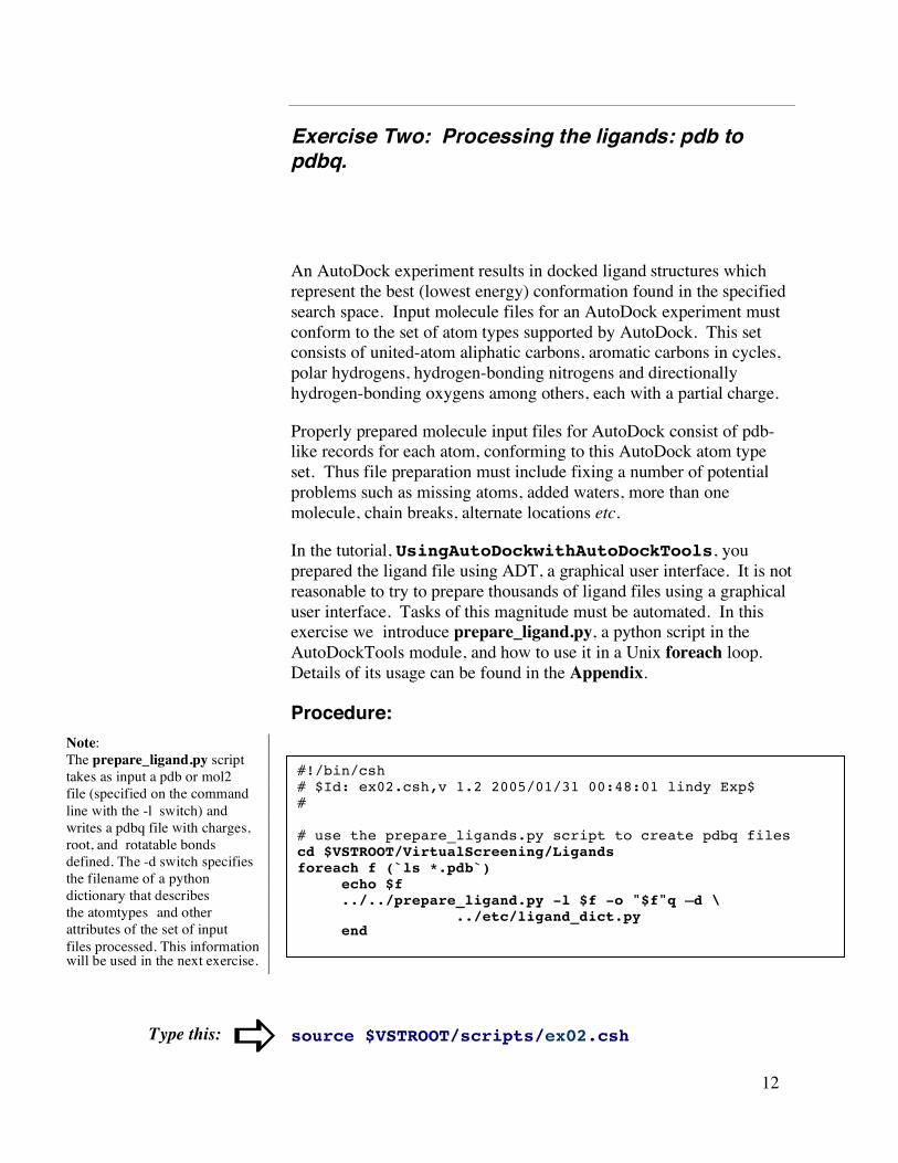
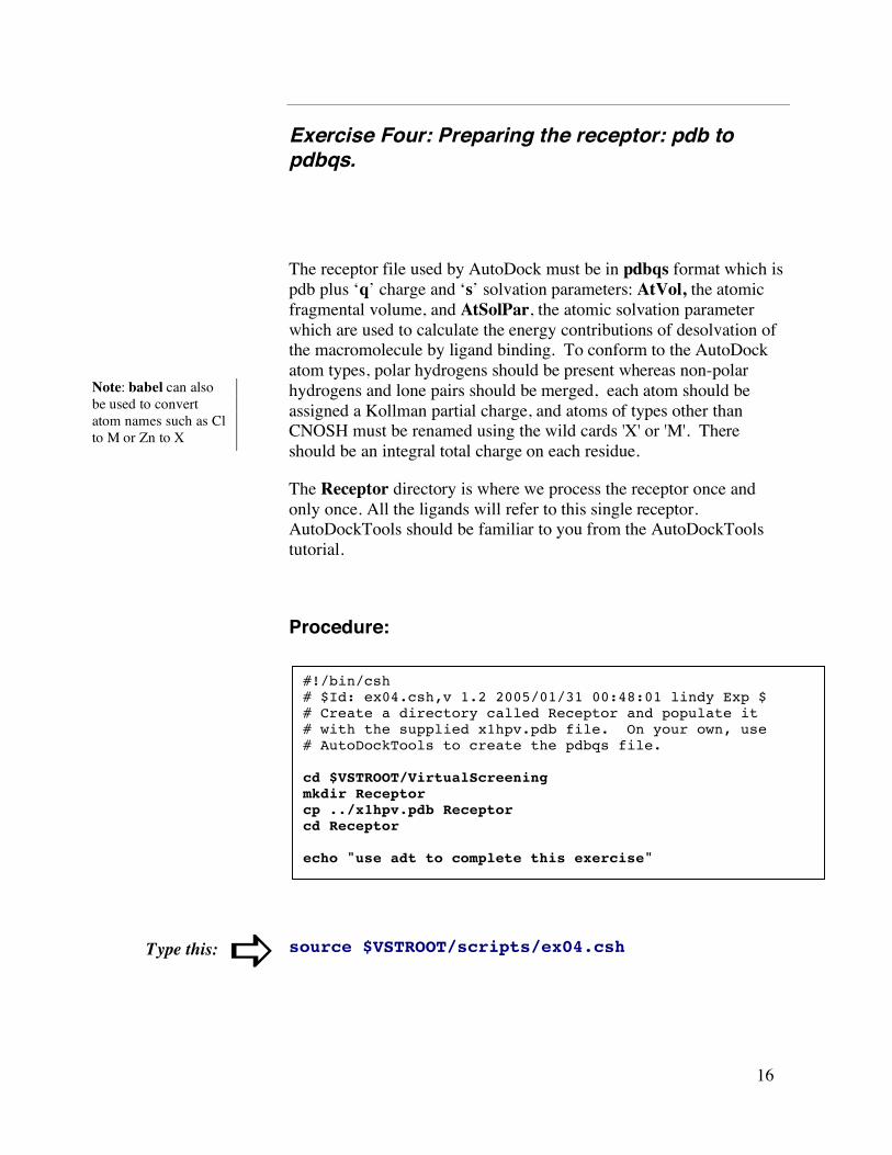
The receptor file used by AutoDock must be in pdbqs format which is pdb plus ‘q’ charge and ‘s’ solvation parameters: AtVol, the atomic fragmental volume, and AtSolPar, the atomic solvation parameter which are used to calculate the energy contributions of desolvation of the macromolecule by ligand binding. To conform to the AutoDock atom types, polar hydrogens should be present whereas non-polar hydrogens and lone pairs should be merged, each atom should be assigned a Kollman partial charge, and atoms of types other than CNOSH must be renamed using the wild cards 'X' or 'M'. There should be an integral total charge on each residue.

The Receptor directory is where we process the receptor once and only once. All the ligands will refer to this single receptor. AutoDockTools should be familiar to you from the AutoDockTools tutorial.

Procedure:


Note: babel can also be used to convert atom names such as Cl to M or Zn to X

#!/bin/csh # $Id: ex04.csh,v 1.2 2005/01/31 00:48:01 lindy Exp $ # Create a directory called Receptor and populate it # with the supplied x1hpv.pdb file. On your own, use # AutoDockTools to create the pdbqs file. cd $VSTROOT/VirtualScreening mkdir Receptor cp ../x1hpv.pdb Receptor cd Receptor echo "use adt to complete this exercise"

Type this:

17

2. Use adt to add hydrogens, charges, and solvent parameters to the receptor and to write x1hpv.pdbqs. adt14 * ADT -> Grid -> Macromolecule -> Open…(AG3) select x1hpv.pdb click on Open * When processing is complete, type x1hpv.pdbqs into the file browser which opens. Be sure to write the file in the Receptor directory. Don’t close adt because we’ll use it in the next exercise. 3. Add an entry for this section’s procedure to the README file.

Note: Alternatively, this preparation could be done via the prepare_receptor.py script. However, if you are working with a single receptor, you should prepare it interactively to optimize selecting the search space.

tutorial

VSTutorial

$VSTROOT


etc Ligands Receptor

x1hpv.pdbqs


TSRI only start adt like this: For linux: /mgl/prog/share/bin/adt14 For mac: Navigate to Applications folder, find AutoDockTools and double click on it.

18

Exercise Five: Preparing AutoGrid Parameter Files for the library

The grid parameter file tells AutoGrid the types of maps to compute, the location and extent of those maps and specifies pair-wise potential energy parameters. In general, one map is calculated for each element in the ligand plus an electrostatics map. Self-consistent 12-6 Lennard-Jones energy parameters - Rij, equilibrium internuclear separation and epsij, energy well depth - are specified for each map based on types of atoms in the macromolecule. If you want to model hydrogen bonding, this is done by specifying 12-10 instead of 12-6 parameters in the gpf.

For a library of ligands, only one atom map per ligand type is required. Each AutoGrid calculation can create up to 6 atom maps plus the electrostatics map. Thus the total number of AutoGrid jobs required for a ligand library is based on the total number of unique atom types in the library. Specifically if there are n unique atom types in the library, at most n/6 + 1 separate grid parameter files must be prepared and AutoGrid must be run n/6 +1 times.

Procedure:

1. Use adt to write the Grid Parameter Files (gpf):

[If you have just written the macromolecule in Exercise Four, skip this first step:

* Grid -> Macromolecule -> Open…(AG3)]

* Grid -> Open GPF… type in ../../x1hpv.gpf and click Open

* Grid -> Set Map Types -> Directly…(AG3) type in ACHNOS and click Accept * Grid -> Output -> Save GPF…(AG3) type in x1hpv_1.gpf in Receptor directory + click Save * Grid -> Set Map Types -> Directly..(AG3) type in cbFP and click Accept * Grid -> Output -> Save GPF…(AG3)

Note: Make sure that you write the grid parameter files in the Receptor directory.

#!/bin/csh # $Id: ex05.csh,v 1.2 2005/01/31 00:48:01 lindy Exp $ echo "Use adt to complete this exercise (05)"

19

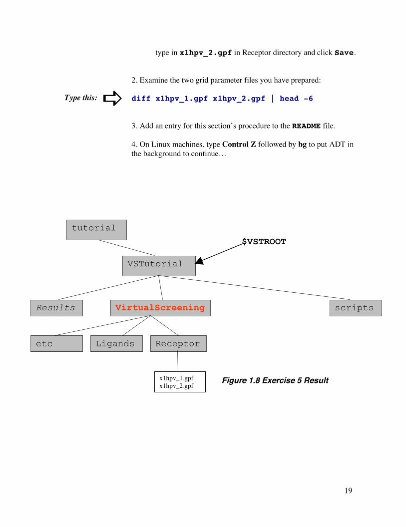
type in x1hpv_2.gpf in Receptor directory and click Save. 2. Examine the two grid parameter files you have prepared: diff x1hpv_1.gpf x1hpv_2.gpf | head -6 3. Add an entry for this section’s procedure to the README file. 4. On Linux machines, type Control Z followed by bg to put ADT in the background to continue…

tutorial

VSTutorial

$VSTROOT



x1hpv_1.gpf x1hpv_2.gpf


Type this:

20

Exercise Six: Calculating atomic affinity maps for a ligand library using AutoGrid.

An essential part of a successful large scale computation experiment such as today’s virtual screening experiment is data organization; that is, a clear directory structure should be used to organize the many input and output files. Our plan places the receptor in a separate directory which is to contain all the AutoGrid affinity maps calculated for this receptor. Under the Receptor directory will be a directory for each ligand. Each ligand directory will contain symbolic links to each map file and to the receptor.pdbqs. Each ligand directory will have its ligand.pdbq file and its unique docking parameter file x1hpv_ligand.dpf.

In this exercise, we invoke autogrid3 twice to calculate the required set of atom maps for x1hpv. We’ll work in the Receptor directory and create the symbolic links for each ligand later.

Procedure:

source $VSTROOT/scripts/ex06.csh 2. Check that the maps are there and check that there are 10 maps . cd $VSTROOT/VirtualScreening/Receptor ls –alt *map ls –alt *map |wc -l 3. Add an entry for this section’s procedure to the README file.

Note: if we were studying more than one receptor, each would be in a separate directory with all the ligands subdirectories under each receptor directory.

#!/bin/csh #$Id: ex06.csh,v 1.1 2004/09/09 00:48:01 lindy Exp $ # 1. Use autogrid3 to create the grid map files: cd $VSTROOT/VirtualScreening/Receptor autogrid3 -p x1hpv_1.gpf -l x1hpv_1.glg autogrid3 -p x1hpv_2.gpf -l x1hpv_2.glg

Type this:

Type this:

Note: the echo utility allows you to ‘see’ what commands are executed by a script. Start it by typing “set echo’. Turn it off by typing ‘unset echo’. Try it here by starting it before sourcing ex06.csh

21

tutorial

VSTutorial

$VSTROOT



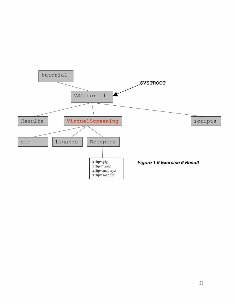
x1hpv.glg x1hpv*.map x1hpv.map.xyz x1hpv.map.fld


22

Exercise Seven: Validating the Protocol with a Positive Control Before we go on and make larger and larger resource and time commitments to the virtual screening experiment, let's make sure in the next exercise that the input files are valid. A docking "job" is a single AutoDock process, which carries out a number of independent docking "runs", each of which begins with the same initial conditions. The various parameters for the docking are usually stored in a docking parameter file, or "DPF". This is passed to AutoDock using a command line flag (-p). Each ligand requires its own docking parameter file. To write the docking parameter files we need for today’s experiment , we will use prepare_dpf.py, a script in AutoDockTools/Utilities. Details of its usage can be found in the Appendix. Procedure: source $VSTROOT/scripts/ex07.csh

Note: each ligand requires its own docking parameter file because some docking parameters are ligand specific: types: atom types in the ligand move: file containing the ligand about: x,y,z coordinates of the center for ligand rotations and translations. ndihe: number of active torsions

#!/bin/csh # $Id: ex07.csh,v 1.3 2005/01/31 02:23:04 lindy Exp $ # Create a directory called ind_x1hpv in the etc # directory: cd $VSTROOT/VirtualScreening/etc mkdir ind_x1hpv cd ind_x1hpv # Populate the directory with the docking input files: cp ../../Ligands/ind.pdbq . ln -s ../../Receptor/x1hpv.pdbqs . ln -s ../../Receptor/x1hpv*map* . # Create the Docking Parameter File with modified # parameters modified to shorten the autodock3 run time # by restricting the search: ../../../prepare_dpf.py -l ind.pdbq -r x1hpv.pdbqs \ -p ga_num_evals=25000 \ -p ga_run=2 # Run autodock3 and examine the output: unlimit stacksize autodock3 -p ind_x1hpv.dpf -l ind_x1hpv.dlg tail ind_x1hpv.dlg

Type this:

Note: We set up symbolic links to the receptor files from each ligand subdirectory. That enables us to have only 1 set of receptor files. You can show symbolic links with “ls –l”

Suggestion: use echo to follow the processing of a single ligand here. Type ‘set echo’ to start and ‘unset echo’ to stop the utility

23

2. You can examine the parameters for a short run contained in this docking parameter file. cat ind_x1hpv.dpf | more 3. Also, you can follow the execution of the autodock job using tail. The ‘-f’ flag makes it follow as new output is written.

tail –f ind_x1hpv.dlg Make sure that “Successful Completion” is found at the end of the file.

4. Add an entry for this section’s procedure to the README file.

tutorial

VSTutorial

$VSTROOT



ind_x1hpv

ind.pdbq x1hpv.pdbqs x1hpv*map* ind_x1hpv.dpf ind_x1hpv.dlg

x1hpv.pdbqs x1hpv*map*


Type this:

Type this:

24

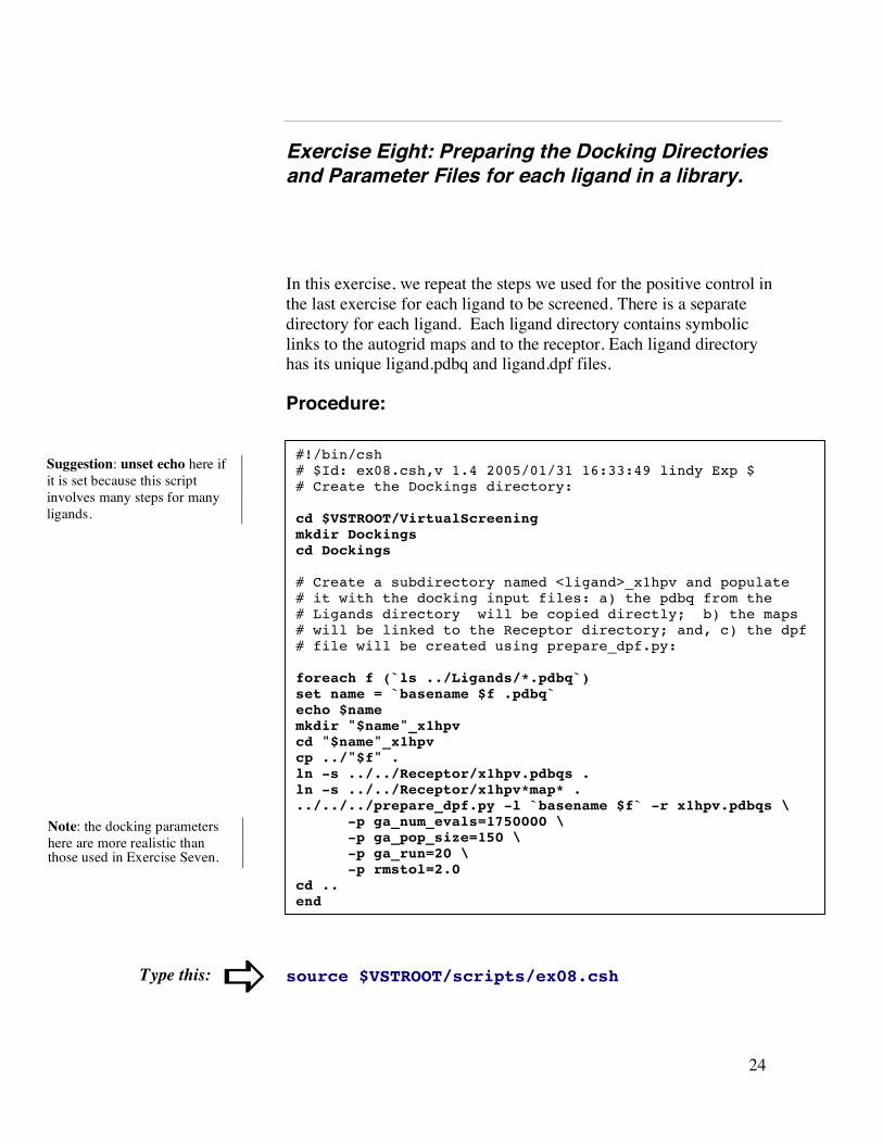
Exercise Eight: Preparing the Docking Directories and Parameter Files for each ligand in a library.

In this exercise, we repeat the steps we used for the positive control in the last exercise for each ligand to be screened. There is a separate directory for each ligand. Each ligand directory contains symbolic links to the autogrid maps and to the receptor. Each ligand directory has its unique ligand.pdbq and ligand.dpf files.

Procedure:


#!/bin/csh # $Id: ex08.csh,v 1.4 2005/01/31 16:33:49 lindy Exp $ # Create the Dockings directory: cd $VSTROOT/VirtualScreening mkdir Dockings cd Dockings

# Create a subdirectory named <ligand>_x1hpv and populate # it with the docking input files: a) the pdbq from the # Ligands directory will be copied directly; b) the maps # will be linked to the Receptor directory; and, c) the dpf # file will be created using prepare_dpf.py: foreach f (`ls ../Ligands/*.pdbq`) set name = `basename $f .pdbq` echo $name mkdir "$name"_x1hpv cd "$name"_x1hpv cp ../"$f" . ln -s ../../Receptor/x1hpv.pdbqs . ln -s ../../Receptor/x1hpv*map* . ../../../prepare_dpf.py -l `basename $f` -r x1hpv.pdbqs \

-p ga_num_evals=1750000 \ -p ga_pop_size=150 \ -p ga_run=20 \ -p rmstol=2.0

cd .. end

Type this:

Suggestion: unset echo here if it is set because this script involves many steps for many ligands.

Note: the docking parameters here are more realistic than those used in Exercise Seven.

25

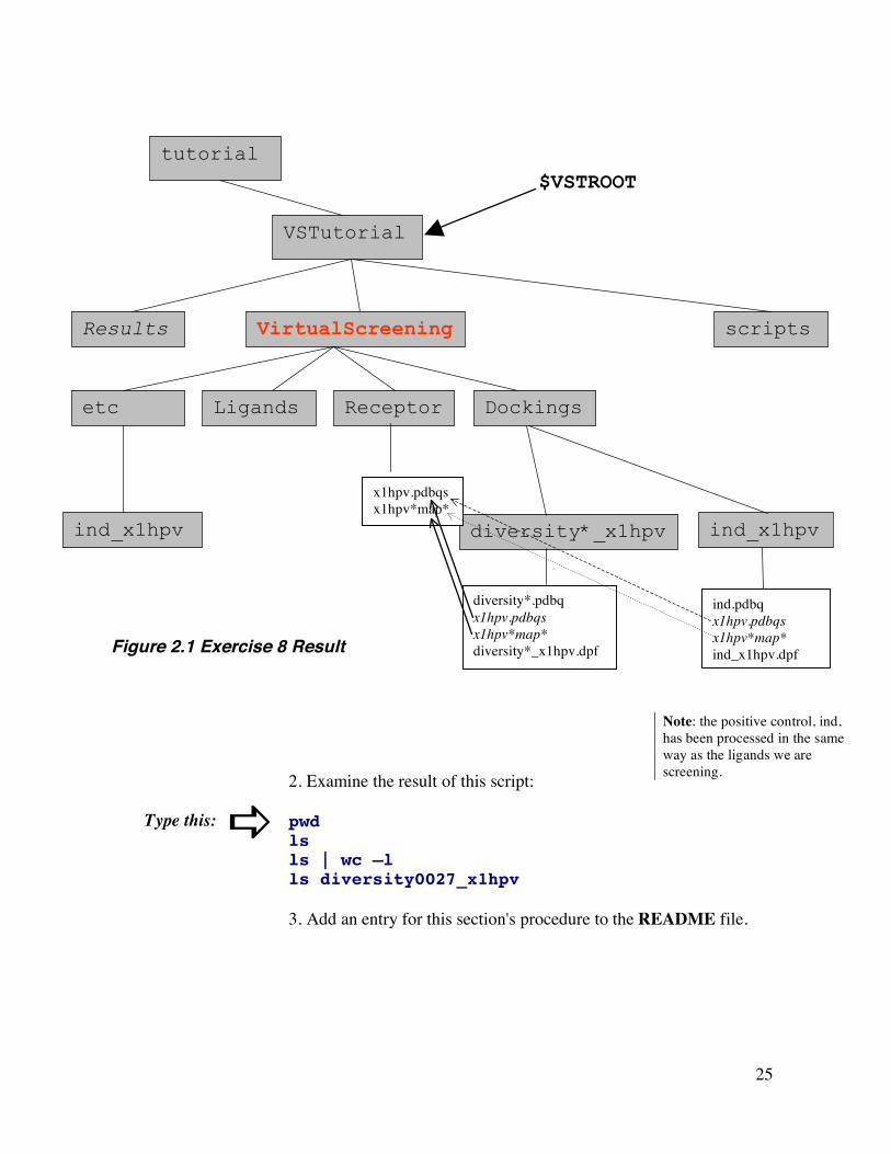
2. Examine the result of this script: pwd ls ls | wc –l ls diversity0027_x1hpv 3. Add an entry for this section's procedure to the README file.

tutorial

VSTutorial

$VSTROOT


etc Ligands Receptor Dockings

ind_x1hpv ind_x1hpv diversity*_x1hpv

diversity*.pdbq x1hpv.pdbqs x1hpv*map* diversity*_x1hpv.dpf

x1hpv.pdbqs x1hpv*map*

ind.pdbq x1hpv.pdbqs x1hpv*map* ind_x1hpv.dpf


Type this:

Note: the positive control, ind, has been processed in the same way as the ligands we are screening.

26

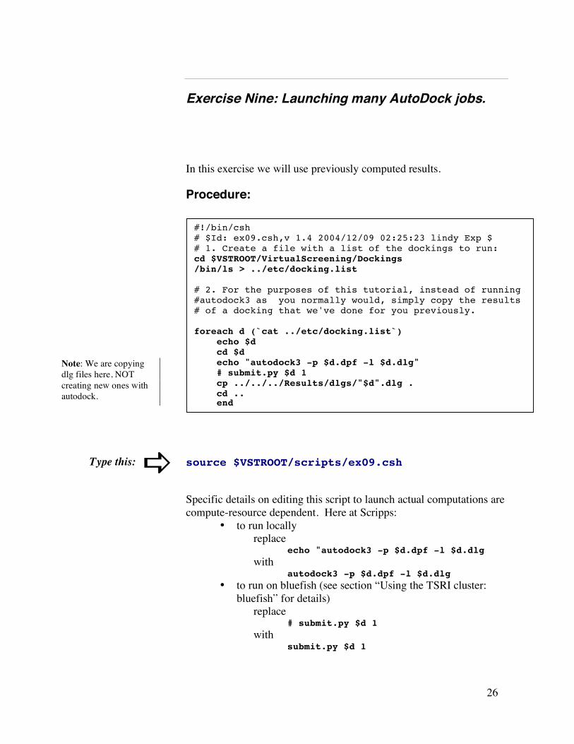
Exercise Nine: Launching many AutoDock jobs.

In this exercise we will use previously computed results.

Procedure:


Specific details on editing this script to launch actual computations are compute-resource dependent. Here at Scripps:

• to run locally replace echo "autodock3 -p $d.dpf -l $d.dlg with

autodock3 -p $d.dpf -l $d.dlg • to run on bluefish (see section “Using the TSRI cluster:

bluefish” for details) replace # submit.py $d 1 with submit.py $d 1

#!/bin/csh # $Id: ex09.csh,v 1.4 2004/12/09 02:25:23 lindy Exp $ # 1. Create a file with a list of the dockings to run: cd $VSTROOT/VirtualScreening/Dockings /bin/ls > ../etc/docking.list # 2. For the purposes of this tutorial, instead of running #autodock3 as you normally would, simply copy the results # of a docking that we've done for you previously. foreach d (`cat ../etc/docking.list`) echo $d cd $d echo "autodock3 -p $d.dpf -l $d.dlg" # submit.py $d 1 cp ../../../Results/dlgs/"$d".dlg . cd .. end

Type this:

Note: We are copying dlg files here, NOT creating new ones with autodock.

27

2. Check that the docking logs exist in the directories under the Dockings directory:

cd $VSTROOT/VirtualScreening/Dockings ls –alt /diversity0027_x1hpv

3. Add a section for this exercise's procedure to the README file.

tutorial

VSTutorial

$VSTROOT




diversity*_x1hpv.dlg

ind_x1hpv.dlg


Type this:

28

Exercise Ten: Identifying the Interesting Results to Analyze.

The first step of analyzing the results is to build a list sorted by energy of the lowest energy docking for each ligand. To do this we first collect all the lig_rec.NNN.dlg to get lig_rec.energies and then sort the lig_rec.energies to create the file lig_rec.energies.sort

Procedure:


#!/bin/csh # $Id: ex10.csh,v 1.3 2005/01/31 02:27:03 lindy Exp $ # # Extract the Free Energy and Docked Energy from the # dlg files. From the docking log files, use grep to # extract the lines containing the binding energy and # docked energy of each complex. Use sed and awk to # process these lines into the final output: cd $VSTROOT/VirtualScreening/Dockings foreach d (`/bin/ls`) echo $d egrep "^USER Estimated Free Energy of Binding| ^USER Final Docked Energy" $d/$d.dlg | sed "N;s/\n//" | awk -v n=$d 'BEGIN {N=n} { print N" "$8" "$15}' > \ $d/$d.energies end # Save the best energy from each docking in a single file # in the pwd directory called all_energies.list: touch ../etc/all_energies.list foreach d ( `/bin/ls` ) echo $d head -1 $d/$d.energies >> ../etc/all_energies.list end # Sort the all_energies.list file to find your best # docking: cd ../etc sort -k3n all_energies.list > all_energies.sort

Type this:

Note: head -1 puts the single best result for each ligand into all_energies.list. You could use head -2 or head -3 to include more results.

Note: -k3n means use field 3 which is the docking energy.

Note: Docking energy is the sum of the intermolecular energy plus the internal energy of the ligand. Binding energy is the sum of the intermolecular energy plus the torsional free energy penalty (0.3113*number of active torsions)

29

2. Take a look at one of the results: cd ../Dockings head diversity1988_x1hpv/diversity1988_x1hpv.energies pwd ls 3. Find your ligands which bind with the lowest energy (best binders) at the top of the list in all_energies.sort. Locate the positive control. Note the ligands that have better energies than it.

cd ../etc head all_energies.sort 4. Add an entry for this section's procedure to the README file.

tutorial

VSTutorial

$VSTROOT




diversity*.energies

ind.energies

all_energies.list all_energies.sort


30

Exercise Eleven: Examine Top Dockings. 1. Start adt: cd ../Dockings adt 2. Setup viewer: * File->Preferences->Set Commands to be Applied on Objects - select colorByAtomType in the Available commands list - click on '>>' - click on 'OK' * File->Browse Commands -click on Pmv in the Select a package: list -select hbondCommands in the Select a module: list -click on Load Module -select msmsCommands -click on Load Module -click on DISMISS 3. Setup receptor: * Read in the file: File->Read Molecule -click on "PDB files (*.pdb)" -select "AutoDock files (pdbqs) (*.pdbqs) -select "x1hpv.pdbqs" * Set center of rotation: -click on pointing finger icon -click on PCOM level: Molecule and select Atom from list -click on bar at right of "printNodeNames" and select centerOnNodes" -draw a box around the water residue (Box should be YELLOW if PCOM level is Atom). * Display msms surface: Compute->Molecular Surface->Compute Molecular Surface -click on OK in MSMS Parameters Panel widget Color->by Atom Type -click on MSMS-MOL and click on OK * Make molecular surface transparent using the DejaVu GUI: -click on Sphere/Cube/Cone (DejaVuGUI) Button -click on + root -click on + x1hpv -select MSMS-MOL

Note: If you have adt running in the background, simply type fg here. TSRI only: start adt using /mgl/prog/share/bin/adt14

Note: If x1hpv.pdbqs is already read it, do not read it in again.

31

-click on Material: Front -change Opacity to .7 -click on Material: None -select root as current object in viewer

* Close the DejaVu GUI: -click on Sphere/Cube/Cone (DejaVuGUI) Button * ADJUST the view: -SHIFT-middle button to zoom in on x1hpv’s water

4. Repeat the following steps for each docking to be evaluated. Here we show the procedure using diversity0629_x1hpv.dlg as an example:

1. Analyze-> Docking Logs->Open -select diversity0619_x1hpv.dlg -click on Open -click on OK 2. Analyze-> Clusterings->Show write a printable version of histogram: -click on histogram’s Edit-> Write -type in this filename: “diversity0619_x1hpv.ps” -click on Save 3. Visualize the lowest energy docked conformation -type ‘d’ in the viewer to turn off depth-cueing -click on lowest energy bin in the histogram to open the player -click on right arrow to set ligand to 1_1 conformation

Assess: -is the ligand in a pocket? -is each atom in the ligand in a chemically favorable position? Show hydrogen bonds: -click on player’s ampersand for play options -click on Build H-bonds and Show Info -Record number of hbonds formed -Display Distance(1.741) or Energy(-5.931)

3. Clea n-up for next docking log -click on Close on ‘diversity0619’ widget -click on File->Exit on ‘diversity0619:rms=2.0 clustering’ histogram -Analyze->Dockings->Clear to delete this docking

5. Add entries for this section’s procedure to the README file

Note: You cannot change the Material properties of a geometry (such as its opacity) if it inherits Materials from its parent. To change this, set the inheritMaterial flag to False: -click on Current Geom Properties button to display a list of checkbuttons for different attributes of the current geometry. -click on inheritMaterial if necessary to turn it off.

32

Using the TSRI cluster: bluefish. All input file preparation should be done on your local computer. The interactive head node on the bluefish cluster is used to transfer the files from your computer to the cluster where the calculations will be carried out. For today’s tutorial, we will demonstrate launching a sample docking and then use previously computed results. We create a tar file of the VSTutorial directory tree: cd /usr/tmp/tutorial tar –czvf VSTutorial.tar.gz VSTutorial Next transfer it to bluefish using sftp. sftp bluefish put VSTutorial.tar.gz exit Log on to bluefish: ssh bluefish Your environment on the bluefish cluster must be set so that autodock3 executable and the python script submit.py are in your path. We will help you do this by editing the .cshrc file in your account on bluefish. Make sure the directory /bluefish/applications/people-b/autodock (which contains the autodock3 executable) is in your path.

set path=($path /bluefish/people-b/applications/autodock) Next uncompress the VSTutorial tree: tar -xzvf VSTutorial.tar.gz We will demonstrate the use of the submit.py script by launching 2 jobs based on the positive control, indinavir. cd VSTutorial/VirtualScreening/etc/ind_x1hpv submit.py ind_x1hpv 2 Notice that the jobs are named ######.bluefish and the name of the script which built the job is given. Here the scripts were named ind_x1hpv001.j and ind_x1hpv002.j. This naming convention is built into submit.py The pbs command qstat is used for tracking job status: qstat | grep yourname

Note: In our usage here of the tar command, we include the verbose flag, -v, to show what is going on.

Type this:

Note: Here we are submitting 2 jobs so that you can try qdel. For a VS experiment submit 1. Submitting more than 1 job is not necessary and only makes analyzing the results unnecessarily complicated.

33

The pbs command qdel is used for removing a job from the queue: qdel ######.bluefish You will receive an email when each job finishes which includes information about whether the job finished successfully or not. For sanity reasons, we will not be launching all the jobs. To do so you would use a foreach loop like this: foreach f (`/bin/ls $VSTROOT/VirtualScreening/Ligands/*.pdbq`)

set name = `basename $f .pdbq` echo $name cd $VSTROOT/VirtualScreening/Receptor/”$name”_x1hpv submit.py $name 10 end

34

Files for exercises:

Input Files: x1hpv.pdb, diversity.sdf, x1hpv.gpf

Results Files

Ligand

<ligand>.pdbq

Macromolecule

x1hpv.pdbqs

AutoGrid

x1hpv_1.gpf, x1hpv_2.gpf x1hpv.*.map, x1hpv.maps.fld,x1hpv.maps.xyz

AutoDock

ind_x1hpv.dpf, ind_x1hpv.dlg, <ligand>_x1hpv.dpf, <ligand>_x1hpv.dlg

35

Appendix A: Usage for AutoDockTools Scripts

The prepare_ligand.py script in AutoDockTools module is customizable via input flags:

prepare_ligand.py –l ligand_filename [vo:d:A:CKU:B:R:Mh]

-l ligand filename (required)

Optional parameters include (defaults are in parentheses):

-v verbose output (none) -o output pdbq_filename (ligandname.pdbq) -d dictionary filename to write summary information of per molecule atomtypes and number of active torsions (none) -A type(s) of repairs to make (none):

bonds hydrogens bonds_hydrogens -C do not add charges (add gasteiger charges) -K add Kollman charges (add gasteiger charges) -U cleanup type, what to merge (nphs_lps) nphs lps “ “ -B types of bonds to allow to rotate (backbone) amide guanidinium amide_guanidinium “ “ -r root (auto) index for root -m mode (automatic) interactive (do not automatically write outputfile)

The prepare_receptor.py script in AutoDockTools module is customizable via input flags:

prepare_receptor.py –r filename ['r:vo:A:CGU:M:'] -r receptor_filename

Note: You can generate any of these usage statements by typing the script name with no input. eg: prepare_ligand.py

36

Optional parameters:" -v verbose output -o pdbqs_filename (receptor_name.pdbqs) -A type(s) of repairs to make (“ “): bonds_hydrogens bonds hydrogens -C do not add charges (add Kollman charges) -G add Gasteiger charges (add Kollman charges)

-U cleanup type, what to merge (nphs_lps) nphs lps “ “ -m mode (automatic) interactive (do not automatically write outputfile)

The prepare_dpf.py script is customizable via input flag (default values are in parenthese)s:

prepare_dpf.py -l ligand_filename –r receptor_filename -l ligand_filename -r receptor_filename Optional parameters:" -v verbose output -o dpf_filename (ligand_receptor.dpf) -i template dpf_filename -p parameter_name=new_value

using autodock for virtual...

Documents