Stephen F. Austin State University Stephen F. Austin State University

SFA ScholarWorks SFA ScholarWorks

Faculty Publications Forestry

2013

Using GIS-Based, Regional Extent Habitat Suitability Modeling to Using GIS-Based, Regional Extent Habitat Suitability Modeling to

Identify Conservation Priority Areas: A Case Study of the Identify Conservation Priority Areas: A Case Study of the

Louisiana Black Bear in East Texas Louisiana Black Bear in East Texas

Christopher E. Comer Arthur Temple College of Forestry and Agriculture, Stephen F. Austin State University, Nacogdoches, Texas 75962, comerce@sfasu.edu

I-Kuai Hung Arthur Temple College of Forestry and Agriculture, Stephen F. Austin State University, hungi@sfasu.edu

Gary Calkins

Dan J. Kaminski

Nathan Garner

Follow this and additional works at: https://scholarworks.sfasu.edu/forestry

Part of the Forest Sciences Commons

Tell us how this article helped you.

Repository Citation Repository Citation Comer, Christopher E.; Hung, I-Kuai; Calkins, Gary; Kaminski, Dan J.; and Garner, Nathan, "Using GIS-Based, Regional Extent Habitat Suitability Modeling to Identify Conservation Priority Areas: A Case Study of the Louisiana Black Bear in East Texas" (2013). Faculty Publications. 278. https://scholarworks.sfasu.edu/forestry/278

This Article is brought to you for free and open access by the Forestry at SFA ScholarWorks. It has been accepted for inclusion in Faculty Publications by an authorized administrator of SFA ScholarWorks. For more information, please contact cdsscholarworks@sfasu.edu.

Management and Conservation

Using GIS-Based, Regional Extent HabitatSuitability Modeling to Identify ConservationPriority Areas: A Case Study of the LouisianaBlack Bear in East Texas

DAN J. KAMINSKI,1,2 Arthur Temple College of Forestry and Agriculture, Stephen F. Austin State University, 419 E. College Street, Nacogdoches,TX 75962, USA

CHRISTOPHER E. COMER, Arthur Temple College of Forestry and Agriculture, Stephen F. Austin State University, 419 E. College Street,Nacogdoches, TX 75962, USA

NATHAN P. GARNER, Texas Parks and Wildlife Department, Region 3 Office, 11942 FM 848, Tyler, TX 75707, USA

I-KUAI HUNG, Arthur Temple College of Forestry and Agriculture, Stephen F. Austin State University, 419 E. College Street, Nacogdoches, TX75962, USA

GARY E. CALKINS, Texas Parks and Wildlife Department, District 6 Wildlife Office, 289 CR 98, Jasper, TX 75951, USA

ABSTRACT State and federal recovery plans mandate that priority areas for future population expansion beidentified within the historical range of the Louisiana black bear (Ursus americanus luteolus). Despite thepresence of potentially suitable habitat in east Texas and expanding populations in adjacent states,quantitative estimates of regional habitat suitability do not exist. We developed a regional extent habitatsuitability index (HSI) model in a geographic information system (GIS) to evaluate year-round habitatrequirements for black bears in the 43,530-km2 south black bear recovery zone in southeastern Texas. Wemeasured hard and soft mast production, understory vegetation density, and tree den availability at 516 surveypoints in 38 habitat classes (82% of the total area in the south recovery zone). We developed geospatialmodels for summer food availability; fall food availability, diversity, and productivity; protection cover, treeden availability, distance to roads, and human development zones and calculated HSI scores per pixel in acontinuous dataset. Habitat suitability scores ranged from 0.00 to 0.76 throughout southeastern Texas.Highly (<1%) and moderately (16%) suitable habitat existed in the region, although most area (84%) wasclassified as marginal or unsuitable habitat. We identified 4 recovery units comprising >20,700 ha (meanHSI¼ 0.5) capable of sustaining viable black bear populations. These units ranged from 62,844 ha to124,808 ha in size and suitable habitat pixels within units ranged from 0.58 to 0.60 in mean HSI scores.Recovery unit scores were comparable to those previously reported for occupied bear range in thesoutheastern United States and acreages of suitable habitat exceeded those estimated to support existingLouisiana black bear populations. � 2013 The Wildlife Society.

KEYWORDS conservation, east Texas, geographic information system (GIS), geospatial modeling, habitat suitabilityindex (HSI), Louisiana black bear, priority areas, Ursus americanus luteolus.

The identification and delineation of priority areas forconservation is a fundamental issue for the effectiveapplication of conservation resources (Gerrard et al. 2001,Clevenger et al. 2002, Felix et al. 2004). For speciesthat require large contiguous habitats or exist at relativelylarge spatial scales, a landscape approach is necessary foradequately identifying appropriate focal areas for conserva-tion (Osborne et al. 2001, Linden et al. 2011). Theavailability of spatial analysis tools like geographic informa-tion systems (GIS) allows conservation managers to assess

habitat availability and quality at a regional or landscape scale(Felix et al. 2004). In occupied areas, wildlife managers mayestimate the suitability of used habitats using radio telemetryor observation data and develop models that extrapolatevalues to a regional scale (Danks and Klein 2002, O’Brienet al. 2005, Rubin et al. 2009). However, in the absence ofthe target species, identifying priority areas poses uniquechallenges for wildlife managers interested in usingestablished modeling techniques for regional reintroductionand monitoring efforts (Didier and Porter 1999).Since the early 1980s, habitat suitability index (HSI)

models have been used to assess environmental impacts towildlife populations, predict habitat suitability (i.e., theability of a given habitat to support a given species) and useby wildlife populations, and facilitate management planning

Received: 12 November 2012; Accepted: 10 June 2013Published: 19 September 2013

1E-mail: danjkaminski@yahoo.com2Present address: 4222 38th Street, Des Moines, IA 50310

The Journal of Wildlife Management 77(8):1639–1649; 2013; DOI: 10.1002/jwmg.611

Kaminski et al. � Modeling Habitat Suitability for Bears 1639

activities (U.S. Fish and Wildlife Service 1980, Allen 1983,Cook and Irwin 1985, Brooks and Temple 1990, van Manenand Pelton 1997, Gurnell et al. 2002). HSI models quantifyhabitat suitability based on known life requisites and habitatrequirements for a given species. Habitat variables (e.g., foodproduction or nest site availability) are evaluated on an indexscale from 0 (unsuitable habitat) to 1 (optimum suitability).Traditional HSI models were designed to evaluate habitatbased on the minimum area necessary for a species toreproduce and survive and to assign a mean suitability scoreto relatively large geographic extents (U.S. Fish andWildlifeService 1980). However, with the development of GIS andadvances in GIS software, computer hardware, and satellitetechnologies, sources of data such as remote satellite andaerial photographic imagery, land-cover models, and digitalelevation models have allowed for the development of moredetailed HSI models and their application to landscape-scale restoration and management efforts (Didier andPorter 1999, McComb et al. 2002, Larson et al. 2003, Felixet al. 2004).Because of the coarseness of most geospatial data,

landscape-scale HSI models are well suited for habitatgeneralists and species with large spatial requirements (Clarket al. 1993, O’Brien et al. 2005). HSI models are commonlyapplied to American black bear (Ursus americanus) pop-ulations to estimate and predict habitat suitability (vanManen 1991, Tankersley 1996, Hersey et al. 2005). Becausemanagement decisions regarding bears are often made at thepopulation level, multiple GIS-based, regional extent modelshave been developed to evaluate suitable habitats for blackbears (van Manen and Pelton 1997, Bowman 1999, Mitchellet al. 2002, Larson et al. 2003). Considering the generalhabitat preferences of black bears, the substantial existingspatial data available regarding black bear habitat suitability,and the sizeable percent of historical range unoccupied byblack bear species in North America (39%; Laliberte andRipple 2004), black bears provide an ideal example towhich GIS tools may be applied to identify priority areasin the absence of a target species or site-specific habitat usedata.East Texas is located within the historical range of the state

and federally threatened Louisiana black bear (Ursusamericanus luteolus). Although once common throughouteastern Texas, the Louisiana black bear had become rare bythe early twentieth century and was considered extirpated bythe 1940s due to indiscriminant and unregulated huntingcoupled with extensive clearing of bottomland hardwoodforests for agriculture (Texas Parks andWildlife Department2005a). The current distribution of the Louisiana black bearis restricted to 3 populations in central and eastern Louisianaand western Mississippi, although recent data suggest thatthese populations are expanding (Black Bear ConservationCoalition, unpublished data). Factors restricting growth andexpansion of the current population include habitat loss,fragmentation, and human-induced mortality (e.g., roadkilland illegal harvest). East Texas is believed to contain some ofthe largest tracts of forested habitat available to but currentlyunoccupied by black bears in the southeast (Wooding

et al. 1996) and may contribute to the future recovery of theLouisiana black bear.In 2009, we initiated a study designed to quantitatively

assess the suitability of east Texas habitats for the Louisianablack bear. Our objective was to identify conservationpriority areas across the landscape capable of sustainingviable populations within the historical range of theLouisiana black bear in east Texas. Because of the largespatial requirements of black bears, increasing numbers ofconfirmed reports of transient bears throughout east Texas,and the general lack of habitat information throughout theregion, our goals were to 1) evaluate east Texas habitats at aregional scale using a statistically valid habitat survey, 2)develop a spatially explicit HSI model using previouslyestablished black bear HSI models and a statisticallyvalidated habitat field survey that could be used to evaluateyear-round habitat requirements for Louisiana black bears inthe absence of site-specific use data, and 3) determinewhether large, contiguous areas of suitable habitats capableof sustaining viable black bear populations exist in east Texas.

STUDY AREA

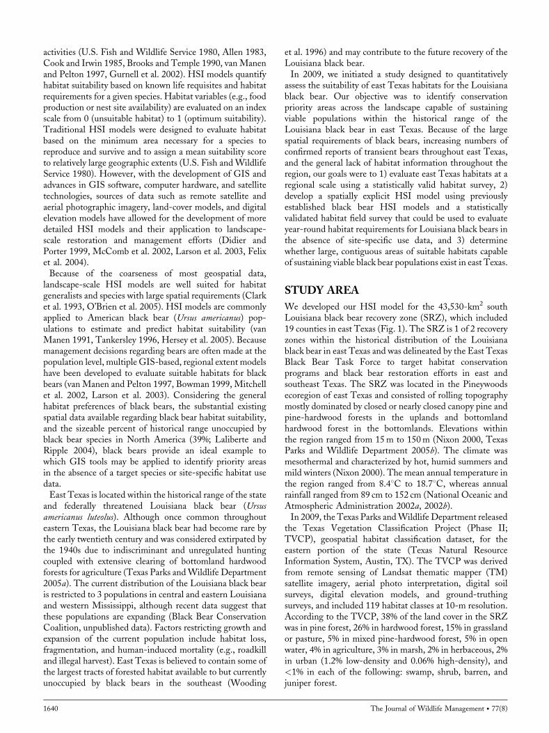
We developed our HSI model for the 43,530-km2 southLouisiana black bear recovery zone (SRZ), which included19 counties in east Texas (Fig. 1). The SRZ is 1 of 2 recoveryzones within the historical distribution of the Louisianablack bear in east Texas and was delineated by the East TexasBlack Bear Task Force to target habitat conservationprograms and black bear restoration efforts in east andsoutheast Texas. The SRZ was located in the Pineywoodsecoregion of east Texas and consisted of rolling topographymostly dominated by closed or nearly closed canopy pine andpine-hardwood forests in the uplands and bottomlandhardwood forest in the bottomlands. Elevations withinthe region ranged from 15m to 150m (Nixon 2000, TexasParks and Wildlife Department 2005b). The climate wasmesothermal and characterized by hot, humid summers andmild winters (Nixon 2000). The mean annual temperature inthe region ranged from 8.48C to 18.78C, whereas annualrainfall ranged from 89 cm to 152 cm (National Oceanic andAtmospheric Administration 2002a, 2002b).In 2009, the Texas Parks andWildlife Department released

the Texas Vegetation Classification Project (Phase II;TVCP), geospatial habitat classification dataset, for theeastern portion of the state (Texas Natural ResourceInformation System, Austin, TX). The TVCP was derivedfrom remote sensing of Landsat thematic mapper (TM)satellite imagery, aerial photo interpretation, digital soilsurveys, digital elevation models, and ground-truthingsurveys, and included 119 habitat classes at 10-m resolution.According to the TVCP, 38% of the land cover in the SRZwas in pine forest, 26% in hardwood forest, 15% in grasslandor pasture, 5% in mixed pine-hardwood forest, 5% in openwater, 4% in agriculture, 3% in marsh, 2% in herbaceous, 2%in urban (1.2% low-density and 0.06% high-density), and<1% in each of the following: swamp, shrub, barren, andjuniper forest.

1640 The Journal of Wildlife Management � 77(8)

METHODS

East Texas Black Bear HSI Model

Our HSI model was based on relationships between liferequisite variables developed by van Manen (1991). The vanManen (1991) model quantified habitat suitability usingmeasures of soft and hard mast production, understoryvegetation density, tree den availability, and human-bearconflict zones. Typically, black bear HSI models includefood, cover, and human impact components (Tankersley1996, Bowman 1999,Mitchell et al. 2002, Larson et al. 2003,Hersey et al. 2005). Although some models have incorpo-rated as many as 20 variables, Mitchell et al. (2002) suggestedthat simpler models consisting of food and denning variablesbetter reflect population-level habitat selection by bears andLarson et al. (2003) suggested that resource availability ismore important to modeling habitat quality for bears thanabiotic components (e.g., slope and aspect). Our basic modelthus included food (CIFOOD), cover (CICOVER), and humanimpact (CIHUMAN IMPACT) component indices (CI)

composed of 8 suitability index (SI) variables: summerfood availability (SISFA), fall food availability (SIFFA), fallfood diversity (SIFFD), fall food productivity (SIFFP),protection cover (SIPC), tree den availability (SITDA),distance to roads (SIR), and human development (SIHD;Table 1).The van Manen (1991) model was designed to assign a

mean HSI score based on empirical habitat data to distinctadministrative boundaries capable of supporting minimumviable populations (MVPs) of black bears (i.e., a populationwith a �95% probability to survive for �100 yr). However,because habitat is generally heterogeneous over largelandscapes, this approach of assigning a single suitabilityscore masks underlying heterogeneity over large study areas.To apply the model at the region-level while maintainingsmall-scale detail, we calculated SI, CI, and HSI scoresseparately for each pixel in a continuous raster dataset basedon empirical field-based habitat data.We used the TVCP to identify potentially suitable habitat

classes for black bears (i.e., classes identified through

Figure 1. Area of eastern Texas designated as the south Louisiana black bear recovery zone and used as the boundary for modeling regional extent habitatsuitability for the Louisiana black bear in 2009–2011.

Kaminski et al. � Modeling Habitat Suitability for Bears 1641

interpretation of the TVCP as potentially capable of meetingthe year-round habitat requirements of black bears) in theSRZ and to select sample sites for field survey. Theavailability of TVCP data allowed us to stratify habitatsurveys by class at the regional level and calculate suitabilityscores per pixel throughout the SRZ. We developed fieldsurveys at the mapping systems level (i.e., Pineywoods: drypine forest or plantation) of the TVCP, which was the finestlevel of resolution and had a produced map accuracy of 75%(A. Treuer-Kuehn, Texas Parks and Wildlife Department,personal communication). Although map accuracy for theTVCP at the most general land-cover level (i.e., pine forest)was 85%, we used the mapping systems level because ofecological differences in habitat composition among classeswithin general land-cover types (i.e., differences betweenyoung pine plantation 1–3m tall and mature Pineywoods:dry pine forest or plantation). However, HSI models arerelative, not absolute, measures of habitat suitability asmultiple, independent life requisite variables contribute tothe overall ability of a given habitat to support a specifiedabundance of a given species. A lower or higher SI score for asingle variable caused by slight differences in habitat betweenthe 2 TVCP levels would only slightly decrease or increasethe overall HSI score (Hersey et al. 2005). We therefore

considered the additional 10% mapping accuracy negligiblefor developing HSI scores and considered the improvedhabitat resolution biologically more important for modelingoverall habitat suitability for black bears at the regional level.

Habitat Field SurveyWe surveyed TVCP habitat classes that were >2,000 ha intotal extent throughout the SRZ and that we identified aspotentially suitable black bear habitats through examinationof the TVCP interpretive booklet (Ludeke et al. 2009). Weidentified 38 of 98 habitat classifications for field surveys,which accounted for 82% of the land area in the region. Wedid not survey most non-habitats (e.g., agriculture and urbanclassifications; 6% of the area in the region), habitats alongthe periphery of the SRZ located outside of the Pineywoodsecoregion (11% of the area), or potentially suitable classesthat were minor components within the Pineywoodsecoregion (1% of the area). We determined number ofsurvey points necessary for collecting reliable data (N) from aclassified map using the binomial probability theory (N¼(Z2� p� q)/E2, where Z¼ 2 from the standard normaldeviate of 1.96 for the 2-sided 95% confidence interval, p isthe expected percent map accuracy, q¼ 100� p, and E is theallowable error; Fitzpatrick-Lins 1981). Using the TVCP

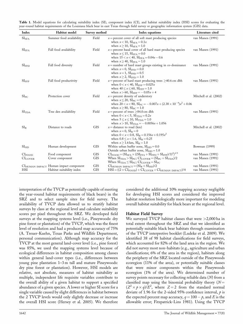
Table 1. Model equations for calculating suitability index (SI), component index (CI), and habitat suitability index (HSI) scores for evaluating theyear-round habitat requirements of the Louisiana black bear in east Texas through field survey or geographic information system (GIS) data.

Index Habitat model Survey method Index equations Literature cited

SISFA Summer food availability Field x¼ percent cover of all soft mast producing species van Manen (1991)when x< 10, SISFA¼ 0.1xwhen x� 10, SISFA¼ 1.0

SIFFA Fall food availability Field x¼ percent basal cover of all hard mast producing species van Manen (1991)when x� 15, SIFFA¼ 0.0when 15< x< 40, SIFFA¼ 0.04x� 0.6when x� 40, SIFFA¼ 1.0

SIFFD Fall food diversity Field x¼ number of hard mast groups existing in co-dominance van Manen (1991)when x¼ 0, SIFFD¼ 0.0when x¼ 1, SIFFD¼ 0.5when x� 2, SIFFD¼ 1.0

SIFFP Fall food productivity Field x¼ percent of hard mast producing trees �40.6 cm dbh van Manen (1991)when 0< x< 40, SIFFP¼ 0.025xwhen 40� x� 60, SIFFP¼ 1.0when x> 60, SIFFP¼� 0.05xþ 4

SIPC Protection cover Field x¼ percent density of understory Mitchell et al. (2002)when x� 20, SIPC¼ 0when 20< x< 80, SIPC¼� 0.007xþ (2.38� 10�4)x2þ 0.06when x� 80, SIPC¼ 1.0

SITDA Tree den availability Field x¼ percent of trees �84.0 cm dbh van Manen (1991)when 0< x< 5, SITDA¼ 0.2xwhen 5� x� 10, SITDA¼ 1.0when x> 10, SITDA¼� 0.0056xþ 1.056

SIR Distance to roads GIS x¼ distance to road (km) Mitchell et al. (2002)when x¼ 0, SIR¼ 0when 0< x< 0.8, SIR¼ 0.156xþ 0.195x2

when 0.8� x< 1.6, SIR¼ 0.25when x� 1.6 km, SIR¼ 1.0

SIHD Human development GIS Within urban buffer zone, SIHD¼ 0.0 Bowman (1999)Outside urban buffer zone, SIHD¼ 1.0

CIFOOD Food component GIS CIFOOD¼ (SISFA� ((SIFFAþ SIFFDþSIFFP)/3)2)1/3 van Manen (1991)

CICOVER Cover component GIS When SITDA> SIPC; CICOVER¼ (SIPCþ SITDA)/2 van Manen (1991)When SITDA� SIPC; CICOVER¼ SIPC

CIHUMAN IMPACT Human impact component GIS CIHUMAN IMPACT¼ (SIRþ SIHD)/2 van Manen (1991)HSI Habitat suitability index GIS HSI¼ ((2�CIFOOD)þCICOVERþCIHUMAN IMPACT)/4 van Manen (1991)

1642 The Journal of Wildlife Management � 77(8)

mapping system accuracy level of 75% for p and an allowableerror of 5%, we calculated a minimumN of 300 survey points.We stratified random points among the 38 selected habitatclasses in ERDAS IMAGINE 9.3 (Intergraph Corporation,Madison, AL) and eliminated those that did not fall withina 3� 3 neighborhood in which all 9 pixels were composed ofthe target class.In addition to calculating the necessary sample size for

assessing the overall accuracy of a classified map, wedetermined the necessary sample size (n) for adequatelysampling each surveyed habitat class. We used a formulabased on the Student’s t-test with a probability of a ofcommitting a type I error and the probability of b ofcommitting a type II error (Zar 2010). We calculatedvariance [s2¼S(x2)� ((S(x)2)/n)], minimum detectabledifference [d¼ (s2/n)� (ta(2),nþ tb(1),n)], and degrees offreedom (n¼ n� 1) for food and cover indices for eachsurveyed habitat class from our data. Using a confidence levelof 0.95 (¼1�a; a¼ 0.05) and power of 0.90 (¼1� b;b¼ 0.10), we calculated n according to the followingequation: n¼ (s2/d2)� (ta(2),nþ tb(1),n)

2.We evaluated SISFA, SIFFA, SIFFD, SIFFP, SIPC, and SITDA

according to van Manen (1991) and Siegmund (Stephen F.Austin State University, unpublished data).We established 10.04-ha fixed-radius plot and 4 5-m2 releve plots at eachsurvey point. We divided each survey point into 4 quartersand located one releve plot in each quarter with the closestcorner of the releve plot located at the closest tree to pointcenter in that quarter.For estimating SISFA, we recorded the species of all soft

mast producing woody plants within each releve plot andestimated percent cover of each in 5% increments. Weaveraged data from the 4 releve plots for each survey point.For estimating SIFFA, SIFFD, SIFFP, and SITDA, we recordedthe species and diameter at breast height (dbh) of all trees�15 cm dbh within the 0.04-ha plot.For estimating SIPC, we measured understory vegetation

density using a vegetation profile board (Nudds 1977). Weconstructed a 30� 200-cm profile board that incorporated acollapsible aluminum frame and a canvas sheet consisting ofalternating 15� 25-cm white and orange rectangle sections.We placed the profile board 15m from point center in eachquarter, in line with the closest tree to point center tominimize bias associated with subjective placement. Werecorded vegetation density by code in 20% increments(1¼ 0–20%, 2¼ 21–40%, 3¼ 41–60%, 4¼ 61–80%, and5¼ 81–100%; Nudds 1977, Griffith and Youtie 1988). Werecorded density codes for every 30� 50-cm section up to200 cm above the ground. We averaged data from the 4profile board readings per height section for each surveypoint. We only analyzed density readings for sections up to100 cm based on the typical maximum shoulder height ofblack bears (van Manen 1991).We measured hard and soft mast production, understory

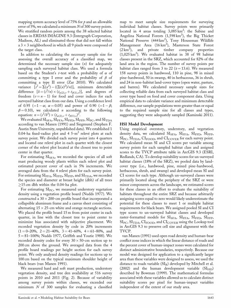
vegetation density, and tree den availability at 516 surveypoints in 2010 and 2011 (Fig. 2). Because of variabilityamong survey points within classes, we exceeded ourminimum N of 300 samples for evaluating a classified

map to meet sample size requirements for surveyingindividual habitat classes. Survey points were primarilylocated in 4 areas totaling 3,085 km2: the Sabine andAngelina National Forests (1,598 km2), the Big ThicketNational Preserve (444 km2), Tony Houseman WildlifeManagement Area (16 km2), Masterson State Forest(2 km2), and private timber company properties(1,025 km2). We evaluated habitat in 38 of 98 habitatclasses present in the SRZ, which accounted for 82% of theland area in the region. The number of survey points perhabitat class ranged from 3 to 22 (�x¼ 13.6). We measured158 survey points in hardwood, 110 in pine, 98 in mixedpine-hardwood, 50 in swamp, 40 in herbaceous, 36 in shrub,and 24 in non-habitat land-cover types (open water, pasture,and barren). We calculated necessary sample sizes forcollecting reliable data from each surveyed habitat class andcover type based on food and cover component data. Usingempirical data to calculate variance and minimum detectabledifference, our sample populations were greater than or equalto the required sample size for all classes and types,suggesting they were adequately sampled (Kaminski 2011).

HSI Model DevelopmentUsing empirical overstory, understory, and vegetationdensity data, we calculated SISFA, SIFFA, SIFFD, SIFFP,SIPC, SITDA, CIFOOD, and CICOVER for each survey point.We calculated mean SI and CI scores per variable amongsurvey points for each sampled habitat class and assignedscores to the TVCP attribute table in ArcGIS 9.3 (ESRI,Redlands, CA). To develop suitability scores for un-surveyedhabitat classes (18% of the SRZ), we pooled data by land-cover type (i.e., hardwood, pine, mixed pine-hardwood,herbaceous, shrub, and swamp) and developed mean SI andCI scores for each type. Although un-surveyed classes wereprimarily located along the periphery of the SRZ or wereminor components across the landscape, we estimated scoresfor these classes in an effort to evaluate the suitability ofhabitats throughout the entire SRZ and because arbitrarilyassigning scores equal to zero would likely underestimate thepotential for these classes to meet 1 or multiple habitatrequirements for black bears. We assigned pooled SI and CItype scores to un-surveyed habitat classes and developedraster-formatted models for SISFA, SIFFA, SIFFD, SIFFP,SIPC, SITDA, CIFOOD, and CICOVER using the Lookup toolin ArcGIS 9.3 to preserve cell size and alignment with theTVCP.vanManen (1991) used open road density and human-bear

conflict zone indices in which the linear distance of roads andthe percent cover of human-impact zones were calculated fordistinct administrative boundaries, respectively. Because ourmodel was designed for application to a significantly largerarea than these variables were designed to assess, we used thedistance to roads variable (SIR) developed by Mitchell et al.(2002) and the human development variable (SIHD)described by Bowman (1999). The mathematical formulasassociated with these variables allowed us to calculate distinctsuitability scores per pixel for human-impact variablesindependent of the extent of our study area.

Kaminski et al. � Modeling Habitat Suitability for Bears 1643

Mitchell et al. (2002) developed the distance to roadsvariable assuming bears avoid areas within 1,600m of roads.Although data regarding the effects of roads on habitatquality for black bears are conflicting (Carr and Pelton 1984,Hellgren et al. 1991, Clark et al. 1993, Fecske et al. 2002,Reynolds-Hogland and Mitchell 2007), we followed vanManen (1991) and assumed that roads have an overallnegative effect through increased traffic-related mortalityand increased efficiency for legal and illegal killing.Reynolds-Hogland and Mitchell (2007) found that blackbears avoided areas �1,600m from gravel roads whenestablishing home ranges and males and females avoidedareas �800m from roads during the summer and fall,respectively. Reynolds-Hogland and Mitchell (2007) con-cluded that roads affect habitat quality at a relatively largespatial scale. We thus buffered all state and county roads in10-m increments out to 800m and from 800m to 1,600musing a single buffer in ArcGIS 9.3. We calculated SI scoresfor buffer rings according to Mitchell et al. (2002) and

converted the model to a raster format with cell size andalignment consistent with the TVCP.Bowman (1999) used a human development variable that

incorporated buffers based on female home range size aroundlow- and high-density urban development. Since the TVCPmodel included low- and high-density urban classes, wedeveloped buffers according to Bowman (1999). van Manen(1991) conceptualized a home range as a circle with thediameter representing the greatest distance an individualbear will travel to meet its year-round habitat requirements.Using this circular home range concept, we estimated a meanfemale Louisiana black bear home range as a circle with adiameter of 3.9 km based on home range estimates for anestablished population of Louisiana black bears in Louisiana(�x¼ 12 km2; Benson and Chamberlain 2007). We createdbuffers of 3.9 km and 1.1 km around all high- andlow-density urban development, respectively, and calculatedSI scores according to Bowman (1999). Because theTVCP high-density urban component incorporated road

Figure 2. Primary study areas and fixed-radius plot locations for conducting field assessments of Louisiana black bear habitat suitability in 2009–2011 insoutheast Texas, USA.

1644 The Journal of Wildlife Management � 77(8)

development, we clipped the high-density urban componentwith incorporated urban polygon data maintained in theTexas Natural Resource Information System (Texas WaterDevelopment Board, Austin, TX) to eliminate redundancyof roads data in our model.

Identification of Recovery Unitsvan Manen (1991) estimated an MVP of black bears to be50–90 individuals based on 1) estimates developed for grizzlybears (U. arctos) by Shaffer (1983) and 2) the estimatedminimum population size necessary to prevent negativegenetic effects related to inbreeding within an MVP for100 years (Franklin 1980, Soule 1980). Based on densityestimates for a black bear population near carrying capacity(�x¼ 1 bear per 2.3 km2), van Manen (1991) estimated that11,500 ha to 20,700 ha of suitable bear habitat were necessaryfor maintaining a MVP. van Manen (1991) further reportedHSI scores of 0.49–0.56 for 3 study units containingestablished black bear populations in the southern Appa-lachians. Using values presented by van Manen (1991), wedefined suitable habitat as pixels with HSI scores �0.50(Garner and Willis 1998). To assess areas capable ofsupporting an MVP of black bears in the SRZ (i.e., recoveryunits), we used a neighborhood analysis of our final HSImodel in ArcGIS 9.3 (Osborne et al. 2001, McCombet al. 2002, Gibson et al. 2004). We used a circular movingwindow to reassign the mean value of pixels within an areathe size of 1 female Louisiana black bear home range (1,950-m radius according to our circular home range estimates) tothe central focal pixel. We exported pixels with mean HSIscores �0.5 and created buffers around pixels of 1,950m toidentify areas within our final HSI where the mean score wasequal to 0.5 (i.e., the area used within each moving windowanalysis). We considered recovery units as areas �20,700 hawith a mean HSI score equal to 0.5 as a conservative estimatefor the minimum area necessary to support a viable bearpopulation according to van Manen (1991).

RESULTS

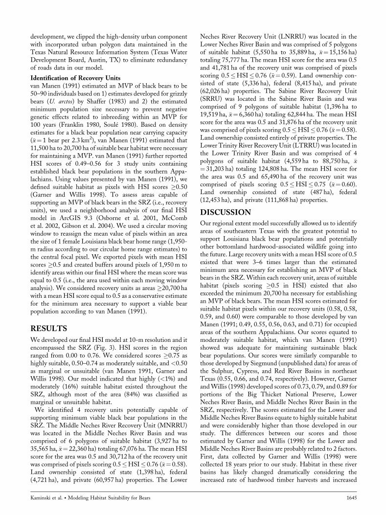
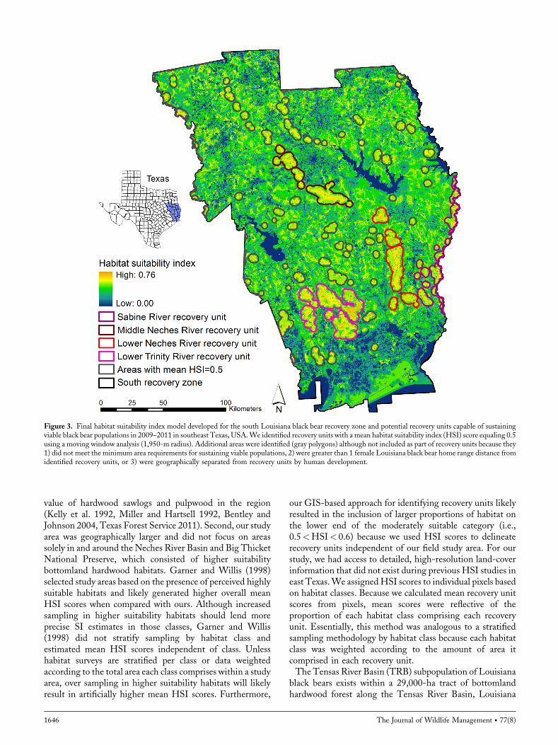
We developed our final HSI model at 10-m resolution and itencompassed the SRZ (Fig. 3). HSI scores in the regionranged from 0.00 to 0.76. We considered scores �0.75 ashighly suitable, 0.50–0.74 as moderately suitable, and <0.50as marginal or unsuitable (van Manen 1991, Garner andWillis 1998). Our model indicated that highly (<1%) andmoderately (16%) suitable habitat existed throughout theSRZ, although most of the area (84%) was classified asmarginal or unsuitable habitat.We identified 4 recovery units potentially capable of

supporting minimum viable black bear populations in theSRZ. The Middle Neches River Recovery Unit (MNRRU)was located in the Middle Neches River Basin and wascomprised of 6 polygons of suitable habitat (3,927 ha to35,565 ha, �x¼ 22,360 ha) totaling 67,076 ha. The mean HSIscore for the area was 0.5 and 30,712 ha of the recovery unitwas comprised of pixels scoring 0.5�HSI� 0.76 (�x¼ 0.58).Land ownership consisted of state (1,398 ha), federal(4,721 ha), and private (60,957 ha) properties. The Lower

Neches River Recovery Unit (LNRRU) was located in theLower Neches River Basin and was comprised of 5 polygonsof suitable habitat (5,550 ha to 35,889 ha, �x¼ 15,156 ha)totaling 75,777 ha. The mean HSI score for the area was 0.5and 41,781 ha of the recovery unit was comprised of pixelsscoring 0.5�HSI� 0.76 (�x¼ 0.59). Land ownership con-sisted of state (5,336 ha), federal (8,415 ha), and private(62,026 ha) properties. The Sabine River Recovery Unit(SRRU) was located in the Sabine River Basin and wascomprised of 9 polygons of suitable habitat (1,396 ha to19,519 ha, �x¼ 6,360 ha) totaling 62,844 ha. The mean HSIscore for the area was 0.5 and 31,876 ha of the recovery unitwas comprised of pixels scoring 0.5�HSI� 0.76 (�x¼ 0.58).Land ownership consisted entirely of private properties. TheLower Trinity River Recovery Unit (LTRRU) was located inthe Lower Trinity River Basin and was comprised of 4polygons of suitable habitat (4,559 ha to 88,750 ha, �x¼ 31,203 ha) totaling 124,808 ha. The mean HSI score forthe area was 0.5 and 65,490 ha of the recovery unit wascomprised of pixels scoring 0.5�HSI� 0.75 (�x¼ 0.60).Land ownership consisted of state (487 ha), federal(12,453 ha), and private (111,868 ha) properties.

DISCUSSION

Our regional extent model successfully allowed us to identifyareas of southeastern Texas with the greatest potential tosupport Louisiana black bear populations and potentiallyother bottomland hardwood-associated wildlife going intothe future. Large recovery units with a meanHSI score of 0.5existed that were 3–6 times larger than the estimatedminimum area necessary for establishing an MVP of blackbears in the SRZ.Within each recovery unit, areas of suitablehabitat (pixels scoring �0.5 in HSI) existed that alsoexceeded the minimum 20,700 ha necessary for establishingan MVP of black bears. The mean HSI scores estimated forsuitable habitat pixels within our recovery units (0.58, 0.58,0.59, and 0.60) were comparable to those developed by vanManen (1991; 0.49, 0.55, 0.56, 0.63, and 0.71) for occupiedareas of the southern Appalachians. Our scores equated tomoderately suitable habitat, which van Manen (1991)showed was adequate for maintaining sustainable blackbear populations. Our scores were similarly comparable tothose developed by Siegmund (unpublished data) for areas ofthe Sulphur, Cypress, and Red River Basins in northeastTexas (0.55, 0.66, and 0.74, respectively). However, GarnerandWillis (1998) developed scores of 0.73, 0.79, and 0.89 forportions of the Big Thicket National Preserve, LowerNeches River Basin, and Middle Neches River Basin in theSRZ, respectively. The scores estimated for the Lower andMiddle Neches River Basins equate to highly suitable habitatand were considerably higher than those developed in ourstudy. The differences between our scores and thoseestimated by Garner and Willis (1998) for the Lower andMiddle Neches River Basins are probably related to 2 factors.First, data collected by Garner and Willis (1998) werecollected 18 years prior to our study. Habitat in these riverbasins has likely changed dramatically considering theincreased rate of hardwood timber harvests and increased

Kaminski et al. � Modeling Habitat Suitability for Bears 1645

value of hardwood sawlogs and pulpwood in the region(Kelly et al. 1992, Miller and Hartsell 1992, Bentley andJohnson 2004, Texas Forest Service 2011). Second, our studyarea was geographically larger and did not focus on areassolely in and around the Neches River Basin and Big ThicketNational Preserve, which consisted of higher suitabilitybottomland hardwood habitats. Garner and Willis (1998)selected study areas based on the presence of perceived highlysuitable habitats and likely generated higher overall meanHSI scores when compared with ours. Although increasedsampling in higher suitability habitats should lend moreprecise SI estimates in those classes, Garner and Willis(1998) did not stratify sampling by habitat class andestimated mean HSI scores independent of class. Unlesshabitat surveys are stratified per class or data weightedaccording to the total area each class comprises within a studyarea, over sampling in higher suitability habitats will likelyresult in artificially higher mean HSI scores. Furthermore,

our GIS-based approach for identifying recovery units likelyresulted in the inclusion of larger proportions of habitat onthe lower end of the moderately suitable category (i.e.,0.5<HSI< 0.6) because we used HSI scores to delineaterecovery units independent of our field study area. For ourstudy, we had access to detailed, high-resolution land-coverinformation that did not exist during previous HSI studies ineast Texas.We assignedHSI scores to individual pixels basedon habitat classes. Because we calculated mean recovery unitscores from pixels, mean scores were reflective of theproportion of each habitat class comprising each recoveryunit. Essentially, this method was analogous to a stratifiedsampling methodology by habitat class because each habitatclass was weighted according to the amount of area itcomprised in each recovery unit.The Tensas River Basin (TRB) subpopulation of Louisiana

black bears exists within a 29,000-ha tract of bottomlandhardwood forest along the Tensas River Basin, Louisiana

Figure 3. Final habitat suitability index model developed for the south Louisiana black bear recovery zone and potential recovery units capable of sustainingviable black bear populations in 2009–2011 in southeast Texas, USA.We identified recovery units with a mean habitat suitability index (HSI) score equaling 0.5using a moving window analysis (1,950-m radius). Additional areas were identified (gray polygons) although not included as part of recovery units because they1) did not meet the minimum area requirements for sustaining viable populations, 2) were greater than 1 female Louisiana black bear home range distance fromidentified recovery units, or 3) were geographically separated from recovery units by human development.

1646 The Journal of Wildlife Management � 77(8)

(Benson and Chamberlain 2007). Bowman (1999) estimatedhabitat suitability for the TRB to be 0.74 (99.2% CI¼0.56–0.92) using the van Manen (1991) HSI. Recent reportsestimated this population at 294 bears (Hooker 2010).Considering the high population density of the TRBsubpopulation, relatively similar or smaller geographic size ofthe TRB compared with our recovery units, and relativelysimilar habitat of the TRB compared with our recovery units(e.g., bottomland hardwood forest; Benson andChamberlain 2007), we expect that our recovery units aremore than adequate for establishing sustainable populationsof black bears in east Texas. Notably, high rates ofagricultural food use by bears in the TRB were documentedand probably contributed to the high density of thepopulation (Benson and Chamberlain 2006). Agriculturecomprised approximately 4% of the land cover in the SRZand likely will not contribute greatly to the year-roundnutrition of black bears in the region. This is ultimatelyadvantageous because agricultural food use is likely tonegatively affect populations through increased negativehuman-bear interactions (van Manen 1991). However,potential population densities and abundance in the SRZmay be lower than those documented in the TRB as a result.Our recovery units consisted of multiple suitable habitat

polygons (mean HSI¼ 0.5) connected by patches ofcontiguous forest typically no further apart than the meanfemale Louisiana black bear home range size (vanManen 1991). The diameter of the mean female Louisianablack bear home range is a conservative estimate for themaximum travel distance of black bears because most blackbear populations in the southeastern United States haveconsiderably larger home range sizes (up to 55 km2) thanthose documented in the TRB (Garshelis and Pelton 1981,Hellgren and Vaughan 1987, Maehr et al. 2003, Dobeyet al. 2005, Moyer et al. 2007). We selected polygonsconnected by contiguous forested habitat to ensure thatappropriate habitat linkages existed among polygonscomprising recovery units (Kindall and van Manen 2007).Although connecting habitats did not meet the year-roundhabitat requirements of black bears, they typically met therequirements for summer food availability and protectioncover. Seasonal shifts in home range are common amongblack bears as they exploit seasonally available food sources(Beeman and Pelton 1980, Graber and White 1983, Garnerand Vaughan 1988, Hellgren and Vaughan 1988) and denseprotection cover is essential for hibernating bears in theabsence of suitable tree dens (Weaver and Pelton 1994, Oliet al. 1997). Thus, these areas may provide seasonal resourcesfor black bear populations in addition to those found withinour delineated recovery units.Compared to assessments of habitat suitability in the

region based entirely on remotely sensed data (Kaminski2011, Morzillo et al. 2011), our analysis resulted in aconsiderably smaller proportion of the area being classifiedas suitable habitat (17% vs. 32% and 73%, respectively).Although suitability modeling based entirely on remotelysensed data may provide useful information whenagency resources limit empirical survey effort (Clevenger

et al. 2002), conclusions should be regarded with caution andverified using independent data (Mitchell et al. 2002). Forinstance, Morzillo et al. (2011) concluded that federal landswere capable of supporting viable bear populations in eastTexas. Based on our field results, federal lands in east Texasgenerally produced marginal suitability scores because pineplantations were the predominant land-cover type and lackednecessary resources to support viable bear populations. Ingeneral, suitability scores assigned a priori to generalizedhabitat classes (i.e., pine or hardwood) differed from scoresbased on field assessments of the TVCP habitat classes by16% to 47%, with consistent overestimation of suitability forhardwood types in particular (Kaminski 2011). These resultsemphasize the utility of using field data to verify assumptionsabout habitat suitability from remotely sensed data.The strength of our modeling approach was that we

selected model variables that were reflective of known blackbear habitat use and could be evaluated across a broadgeographic region independent of an established population.Geospatial modeling is limited by the availability of GISdatasets applicable to a given species’ ecological requirements(Gibson et al. 2004). However, the datasets that weincorporated may be obtained through habitat survey andmodeling of common urban spatial data. Gibson et al. (2004)noted the rarity of studies in the literature that combinedgeospatial modeling with field-based habitat assessment andrecommended that this approach would likely be anadvantageous, yet costly, modeling method for fine-scalehabitat assessment. In the case of our study, we were assistedby the availability of the high-quality and fine-resolutionTVCP spatial dataset. However, as Gibson et al. (2004)suggested, we were required to invest 2 field seasons togenerate statistically adequate sample sizes for our habitatsurveys. Ultimately, the additional cost resulted in thedevelopment of a fine-resolution HSI model capable ofidentifying priority areas at the regional level. For Texas orother states with detailed digital land-cover databases, thisapproach could be used to develop regional extent suitabilitymodels for any species for which habitat requirements arewell understood.The absence of an established black bear population in east

Texas meant our HSI model lacked model validation fordeveloping a level of precision according to Mitchell et al.(2002). Mitchell et al. (2002) considered an HSI model ahypothesis and model validation to be an evaluation of themodel with independent home range or telemetry data. Wederived our model assumptions from long-term monitoringof established black bear populations and well-documentedblack bear habitat requirements. vanManen (1991) evaluatedHSI scores with home range data and showed that the HSIwas reflective of habitat use in the southern Appalachians.Additionally, we developed our SI, CI, and HSI scores fromempirical habitat data and evaluated them using standardsampling statistics. Although we derived our HSI scoresfrom empirical habitat data, scores do not reflect actual blackbear use in east Texas. However, Mitchell and Powell (2003)noted that bias associated with black bear HSI models waslikely minimal because 1) a large number of component-

Kaminski et al. � Modeling Habitat Suitability for Bears 1647

based HSI models exist that approximate the relationshipbetween black bears and their habitat, 2) HSI estimates arenot exceedingly sensitive to any 1 component, and 3) the useof multiple, relatively independent component indices limitsdirectional bias in applications of the full HSI. Thus, weregard the combination of using previously validated HSImodels and statistically validated habitat survey to be suitablefor identifying potential recovery units in areas lacking anestablished black bear population or site-specific use data.

MANAGEMENT IMPLICATIONS

Our results indicate that areas of large, contiguous forestedhabitat capable of meeting the year-round habitat require-ments of Louisiana black bears and sustaining viablepopulations exist within the historical range of the subspeciesin east Texas. The identification of recovery units based onthe ecological requirements of black bears provides areas inwhich future management, research, public outreach, orreintroduction efforts may be targeted. The recovery units wepresented are each comprised of >80% private landowner-ship, which emphasizes the need to incorporate publicoutreach and education with management actions, and todevelop incentive programs for private landowners toconserve high-quality habitats for the long-term. Collabo-ration with private landowners to implement uneven-agedand/or longer rotation forest management could boost fallfood variables in critical bottomland hardwood habitats andimprove overall HSI estimates. However, because forestmanagement practices and recovery-unit HSI estimates ineast Texas are similar to those in areas with established blackbear populations in the southeastern United States, wesuggest that habitat fragmentation and the conversion offorestlands to less renewable resources poses a greater risk tothe sustainability of recovery units. Thus managementactions should focus on preserving large contiguous forestedhabitats free of human disturbance in and around recoveryunits.

ACKNOWLEDGMENTS

Primary funding for this project was provided by the TexasParks and Wildlife Department, with additional significantcontributions from the Black Bear Conservation Coalition,the Coypu Foundation, and the East Texas Black Bear TaskForce. D. Kaminski received funding from the ArthurTemple College of Forestry and Agriculture, Stephen F.Austin State University, and from the USDA McIntire-Stennis Program. We thank D. Scognamillo and D. Ungerfor providing GIS support and review of our HSI model, S.Lange for providing spatial data, and J. Williams forproviding technical support throughout the duration of thisstudy. We thank D. Coble and W. Conway for providingassistance with statistics and study design. Land access forthis study was provided by the U.S. Forest Service (J. Engleand E. Taylor), Big Thicket National Preserve (D. Roemerand B. Lockwood), Campbell Timberland ManagementLLC (B. Stansfield, D. Dietz, and M. Richardson),and Hancock Forest Management (C. Nichol). CampbellTimberland Management LLC also provided housing for

our field technicians. We thank S. Payne for assisting withfield data collection.We also thank our referees for providingcomments that improved our manuscript.

LITERATURE CITEDAllen, A. W. 1983. Habitat suitability index models: beaver. U.S. Fish andWildlife Service FWS/OBS-82/10.30 Revised, Washington, D.C., USA.

Beeman, L. E., and M. R. Pelton. 1980. Seasonal foods and feeding ecologyof black bears in the Smoky Mountains. Proceedings of the InternationalConference on Bear Research and Management 4:141–147.

Benson, J. F., and M. J. Chamberlain. 2006. Food habits of Louisiana blackbears (Ursus americanus luteolus) in two subpopulations of the Tensas RiverBasin. American Midland Naturalist 156:188–197.

Benson, J. F., and M. J. Chamberlain. 2007. Space use and habitat selectionby female Louisiana black bears in the Tensas River Basin of Louisiana.Journal of Wildlife Management 71:117–126.

Bentley, J. W., and T. G. Johnson. 2004. Eastern Texas harvest andutilization study, 2003. U.S. Forest Service Resource Bulletin SRS-97,Southern Research Station, Asheville, North Carolina, USA.

Bowman, J. L. 1999. An assessment of habitat suitability and humanattitudes for black bear restoration inMississippi. Dissertation,MississippiState University, Starkville, USA.

Brooks, B. L., and S. A. Temple. 1990.Habitat availability and suitability forloggerhead shrikes in the upper Midwest. American Midland Naturalist123:75–83.

Carr, P. C., andM. R. Pelton. 1984. Proximity of adult female black bears tolimited access roads. Proceedings of the Southeastern Association of Fishand Wildlife Agencies 38:70–77.

Clark, J. D., J. E. Dunn, and K. G. Smith. 1993. A multivariate model offemale black bear habitat use for a geographic information system. Journalof Wildlife Management 57:519–526.

Clevenger, A. P., J. Wierzchowski, B. Chruszcz, and K. Gunson. 2002.GIS-generated, expert-based models for identifying wildlife habitatlinkages and planning mitigation passages. Conservation Biology 16:503–514.

Cook, J. G., and L. L. Irwin. 1985. Validation and modification of a habitatsuitability model for pronghorns. Wildlife Society Bulletin 13:440–448.

Danks, F. S., and D. R. Klein. 2002. Using GIS to predict potential wildlifehabitat: a case study of muskoxen in northern Alaska. International Journalof Remote Sensing 23:4611–4632.

Didier, K. A., and W. F. Porter. 1999. Large-scale assessment of potentialhabitat to restore elk to New York State. Wildlife Society Bulletin 27:409–418.

Dobey, S., D. V. Masters, B. K. Scheick, J. D. Clark, M. R. Pelton, andM. E. Sunquist. 2005. Ecology of Florida black bears in the Okefenokee-Osceola ecosystem. Wildlife Monographs 158:1–41.

Fecske, D. M., R. E. Barry, F. L. Precht, H. B. Quigley, S. L. Bittner, andT. W. Webster. 2002. Habitat use by female black bears in westernMaryland. Southeastern Naturalist 1:77–92.

Felix, A. B., H. Campa, III, K. F. Millenbah, S. R. Winterstein, andW. E.Moritz. 2004. Development of landscape-scale habitat-potential modelsfor forest wildlife planning and management. Wildlife Society Bulletin32:795–806.

Fitzpatrick-Lins, K. 1981. Comparison of sampling procedures and dataanalysis for land-use and land-cover map. Photogrammetric Engineeringand Remote Sensing 47:343–351.

Franklin, I. R. 1980. Evolutionary change in small populations. Pages 135–150 in M. E. Soule and B. A. Wilcox, editors. Conservation biology: anevolutionary-ecological perspective. Sinauer Associates, Sunderland,Massachusetts, USA.

Garner, N. P., and M. R. Vaughan. 1988. Black bears use of abandonedhome sites in ShenandoahNational Park. Proceedings of the InternationalConference on Bear Research and Management 7:151–157.

Garner, N. P., and S. E.Willis. 1998. Suitability of habitats in east Texas forblack bears. Texas Parks and Wildlife Department, Tyler, USA.

Garshelis, D. L., and M. R. Pelton. 1981. Movements of black bears in theGreat Smoky Mountains National Park. Journal of Wildlife Management45:912–925.

Gerrard, R., P. Stin, R. Church, and M. Gilpin. 2001. Habitat evaluationusing GIS: a case study applied to the San Joaquin kit fox. Landscape andUrban Planning 52:239–255.

1648 The Journal of Wildlife Management � 77(8)

Gibson, L. A., B. A. Wilson, D. M. Cahill, and J. Hill. 2004. Spatialprediction of rufous bristlebird habitat in a coastal heathland: a GIS-basedapproach. Journal of Applied Ecology 41:213–223.

Graber, D. M., and M. White. 1983. Black bear food habits in YosemiteNational Park. Proceedings of the International Conference on BearResearch and Management 5:1–10.

Griffith, B., and B. A. Youtie. 1988. Two devices for estimating foliagedensity and deer hiding cover. Wildlife Society Bulletin 16:206–210.

Gurnell, J.,M. J. Clark, P.W.W. Lurz,M.D. F. Shirley, and S. P. Rushton.2002. Conserving red squirrels (Sciurus vulgaris): mapping and forecastinghabitat suitability using a geographic information systems approach.Biological Conservation 105:53–64.

Hellgren, E. C., and M. R. Vaughan. 1987. Home range and movements ofwinter-active black bears in the Great Dismal Swamp. Proceedings of theInternational Conference on Bear Research and Management 7:227–234.

Hellgren, E. C., and M. R. Vaughan. 1988. Seasonal food habits of blackbears in Great Dismal Swamp, Virginia-North Carolina. Proceedings ofthe Southeastern Association of Fish and Wildlife Agencies 42:295–305.

Hellgren, E. C.,M. R. Vaughan, and D. F. Stauffer. 1991.Macrohabitat useby black bears in a southeastern wetland. Journal of Wildlife Management55:442–448.

Hersey, K. R., A. S. Edwards, and J. D. Clark. 2005. Assessing Americanblack bear habitat in the Mobile-Tensaw Delta of southwestern Alabama.Ursus 16:245–254.

Hooker, M. J. 2010. Estimating population parameters of the Louisianablack bear in the Tensas River Basin, Louisiana, using robust designcapture-mark-recapture. Thesis, University of Tennessee, Knoxville,USA.

Kaminski, D. J. 2011. Assessment of the population status and evaluation ofsuitable habitats for the Louisiana black bear (Ursus americanus luteolus) ineast Texas. Thesis, Stephen F. Austin State University, Nacogdoches,Texas, USA.

Kelly, J. F., P. E. Miller, and A. J. Hartsell. 1992. Forest statistics forsoutheast Texas counties—1992. U.S. Forest Service Resource BulletinSO-17, Southern Forest Experimental Station, New Orleans, Louisiana,USA.

Kindall, J. L., and F. T. van Manen. 2007. Identifying habitat linkages forAmerican black bears in North Carolina, USA. Journal of WildlifeManagement 71:487–495.

Laliberte, A. S., and W. J. Ripple. 2004. Range contractions of NorthAmerican carnivores and ungulates. Bioscience 54:123–138.

Larson, M. A., W. D. Dijak, F. R. Thompson, III, and J. J. Millspaugh.2003. Landscape-level habitat suitability models for twelve wildlife speciesin southern Missouri. U.S. Forest Service General Technical Report NC-233. North Central Research Station, St. Paul, Minnesota, USA.

Linden, D. W., H. Campa, III, G. J. Roloff, D. E. Beyer, Jr., and K. F.Millenbah. 2011. Modeling habitat potential for Canada lynx inMichigan. Wildlife Society Bulletin 35:20–26.

Ludeke, K., D. German, and J. Scott. 2009. Texas vegetation classificationproject: interpretive booklet for phase II. Texas Parks and WildlifeDepartment and Texas Natural Resources Information System, Austin,USA.

Maehr, D. S., J. S. Smith, M. W. Cunningham, M. E. Barnwell, J. L.Larkin, and M. A. Orlando. 2003. Spatial characteristics of an isolatedFlorida black bear population. Southeastern Naturalist 2:433–446.

McComb, W. C., M. T. McGrath, T. A. Spies, and D. Vesely. 2002.Models for mapping potential habitat at landscape scales: an example usingnorthern spotted owl. Forest Science 48:203–216.

Miller, P. E., and A. J. Hartsell. 1992. Forest statistics for east Texascounties—1992. U.S. Forest Service Resource Bulletin SO-17, SouthernForest Experiment Station, New Orleans, Louisiana, USA.

Mitchell, M. S., and R. A. Powell. 2003. Response of black bears to forestmanagement in the southern Appalachian mountains. Journal of WildlifeManagement 67:692–705.

Mitchell,M. S., J.W. Zimmerman, and R. A. Powell. 2002. Test of a habitatsuitability index for black bears in the southern Appalachians. WildlifeSociety Bulletin 30:794–808.

Morzillo, A. T., J. R. Ferrari, and J. Liu. 2011. An integration of habitatevaluation, individual based modeling, and graph theory for a potential

black bear population recovery in southeastern Texas, USA. LandscapeEcology 26:69–81.

Moyer, M. A., J. W. McCown, and M. K. Oli. 2007. Factors influencinghome-range size of female Florida black bears. Journal of Mammalogy88:468–476.

National Oceanic and Atmospheric Administration. 2002a. Precipitation.Climatography of the United States No. 85. National Climatic DataCenter/NESDIS/NOAA, Asheville, North Carolina, USA.

National Oceanic and Atmospheric Administration. 2002b. Temperature.Climatography of the United States No. 85. National Climatic DataCenter/NESDIS/NOAA, Asheville, North Carolina, USA.

Nixon, E. S. 2000. Trees, shrubs, and woody vines of East Texas. Secondedition. B.L. Cunningham Productions, Nacogdoches, Texas, USA.

Nudds, T. D. 1977. Quantifying the vegetative structure of wildlife cover.Wildlife Society Bulletin 5:113–117.

O’Brien, C. S., S. S. Rosenstock, J. J. Hervert, J. L. Bright, and S. R. Boe.2005. Landscape-level models of potential habitat for Sonoran pronghorn.Wildlife Society Bulletin 33:24–34.

Oli, M. K., H. A. Jacobson, and B. D. Leopold. 1997. Denning ecology ofblack bears in the White River National Wildlife Refuge, Arkansas.Journal of Wildlife Management 61:700–706.

Osborne, P. E., J. C. Alonso, and R. G. Bryant. 2001. Modelling landscape-scale habitat use using GIS and remote sensing: a case study with greatbustards. Journal of Applied Ecology 38:458–471.

Reynolds-Hogland, M. J., and M. S. Mitchell. 2007. Effects of roads onhabitat quality for bears in the southern Appalachians: a long-term study.Journal of Mammalogy 88:1050–1061.

Rubin, E. S., C. J. Stermer, W. M. Boyce, and S. G. Torres. 2009.Assessment of predictive habitat models for bighorn sheep in California’sPeninsular ranges. Journal of Wildlife Management 73:859–869.

Shaffer, M. L. 1983. Determining minimum viable population sizes for thegrizzly bear. International Conference on Bear Research andManagement5:133–139.

Soule, M. E. 1980. Thresholds for survival: maintaining fitness andevolutionary potential. Pages 151–170 in M. E. Soule and B. A. Wilcox,editors. Conservation biology: an evolutionary-ecological perspective.Sinauer Associates, Sunderland, Massachusetts, USA.

Tankersley, R. 1996. Black bear habitat in the southeastern United States: abiometric model of habitat conditions in the southern Appalachians.Thesis, University of Tennessee, Knoxville, USA.

Texas Forest Service. 2011. Texas Forest Service, Texas A&M UniversitySystem. Texas price trends: historical timber price summary from 1984.<http://txforestservice.tamu.edu/main/article.aspx?id¼148>. Accessed15 Nov 2011.

Texas Parks and Wildlife Department. 2005a. East Texas black bearconservation and management plan. Texas Parks and Wildlife Depart-ment, Austin, USA.

Texas Parks and Wildlife Department. 2005b. Pineywoods ecoregion. Page162–177 in S. Bender, S. Shelton, K. C. Bender, and A. Kalmbach,editors. Texas comprehensive wildlife conservation strategy. Texas Parksand Wildlife Department, Austin, USA.

U.S. Fish and Wildlife Service. 1980. Habitat evaluation procedures (HEP)102 ESM. U.S. Fish and Wildlife Service, Washington, D.C., USA.

vanManen, F. T. 1991. A feasibility study for the potential reintroduction ofblack bears into the Big South Fork Area of Kentucky and Tennessee.Tennessee Wildlife Resources Agency Technical Report No. 91-3,Knoxville, USA.

van Manen, F. T., and M. R. Pelton. 1997. A GIS model to predict blackbear habitat use. Journal of Forestry 95:6–12.

Weaver, K. M., and M. R. Pelton. 1994. Denning ecology of black bears inthe Tensas River Basin of Louisiana. Proceedings of the InternationalConference on Bear Research and Management 9:427–433.

Wooding, J. B., J. A. Cox, and M. R. Pelton. 1996. Distribution of blackbears in the southeastern coastal plain. Proceedings of the SoutheasternAssociation of Fish and Wildlife Agencies 48:270–275.

Zar, J. H. 2010. Biostatistical analysis. Fifth edition. Prentice Hall, UpperSaddle River, New Jersey, USA.

Associate Editor: Michael Chamberlain.

Kaminski et al. � Modeling Habitat Suitability for Bears 1649