Using GPU Shaders for Visualization, II

Mike Bailey, Oregon State University mjb@cs.oregonstate.edu

Introduction GPU Shaders are not just for special effects. In [Bailey2009], we looked at some uses for GPU shaders in visualization. In this article, we continue that idea. Because visualization relies so much on high-speed interaction, we use shaders for the same reason we use them in effects programming: appearance and performance. In the drive to understand large, complex data sets, no method should be overlooked. This article describes two additional visualization applications: line integral convolution and terrain bump-mapping. It also comments on the recent (and rapid) changes to OpenGL, and what these mean to educators. Previous Work Using shaders for visualization started with experiments using RenderMan, e.g., [Corrie1993]. Interactive (i.e., graphics hardware-based) GPU Shaders appeared in the early 2000s [Mark2003]. Since then, researchers have pushed them into a variety of applications. Many of these have involved scientific and data visualization using volume rendering [Stegmaier2005], level of detail management [Petrovic2007], volume segmentation [Sherbondy2003], and level sets [Lefohn2003]. Other work has used GPU programming to combine and filter visualization data to show particular features of interest [McCormick2004]. Reading 3D scalar data into a shader Shaders were designed to accept relatively small sets of scene-describing graphics

attributes such as colors, coordinates, vectors, and matrices, as input data. Passing large amounts of general-purpose data into them, such as through uniform variables, is inefficient. It is better to find some way that looks more consistent with the graphics intent of shaders. In this case, an excellent approach is to hide the data in a 3D texture. Textures were designed to store RGBA color values. The most common format for textures, still, is probably the unsigned byte format, specifically created to hold 8-bit color components. However, today’s graphics cards can also use 16- and 32-bit floating point formats to store texture components. Thus, textures can hold any scale of numbers, within the limits of those floating-point formats, that we want. This makes them ideal as a way to hold 3D data for visualization. 2D Line Integral Convolution Line Integral Convolution (LIC) [Cabral1993] is a visualization technique to show flow directions across a 2D field. The method essentially smears an image in the directions of the flow, as shown below in Figures 2-4. The image being smeared is oftentimes a white noise texture (shown in Figure 1), so that the result is a grayscale smear. This listing shows a fragment shader to implement the LIC algorithm. Two textures are being accessed – one for the background image being smeared and one to hold the flow field. If the flow field image is an unsigned byte texture, then the flow velocities must be scaled to fit in the range 0-255 when the texture is being created. Once in the shader, those byte-texture

components will have been scaled into the range 0.-1., and thus must be “un-scaled”. In this case, the flow velocities were packed into a floating-point texture so that the values could be used as-is with no scaling and un-scaling. Because this is a 2D flow field, the x and y velocities are packed into just the red and green texture components. The geometry drawn is a four-vertex 2D quadrilateral. The vertex shader is shown below. The out variable vST is the s and t texture coordinates at this particular vertex, and will eventually be interpolated and sent to the fragment shader via the rasterizer. #version 400 compatibility precision highp float; precision highp int; out vec2 vST; void main( void ) { vST = gl_MultiTexCoord0.st; gl_Position = gl_ModelViewProjectionMatrix * gl_Vertex; }

The code below is the fragment shader. fColor is the color that will fill this pixel. uLength is a uniform variable that controls how many samples are taken in each direction along the flow lines. #version 400 precision highp float; precision highp int; uniform int uLength; uniform sampler2D uImageUnit; uniform sampler2D uFlowUnit; in vec2 vST; out vec4 fColor; void main( void ) { ivec2 res=textureSize( uImageUnit, 0 ); // flow field direction: vec2 st = vST; vec2 v; v = texture( uFlowUnit, st ).xy; v *= ( 1./vec2(res) ); // because velocities go from -1. to +1. // and textures go from 0. to 1. // starting location: st = vST; vec3 color = texture( uImageUnit, st ).rgb; int count = 1;

st = vST; for( int i = 0; i < uLength; i++ ) { st += v; vec3 new = texture( uImageUnit, st ).rgb; color += new; count++; } st = vST; for( int i = 0; i < uLength; i++ ) { st -= v; vec3 new = texture( uImageUnit, st).rgb; color += new; count++; } color /= float(count); fColor = vec4( color, 1. ); }

Figure 1. White Noise Texture used as

the Input Image

Figure 2. LIC with a Length of 10

Figure 3. LIC with a Length of 30

Figure 4. LIC with a Length of 100

By using the highly-parallelized fragment processors, the interactive performance is excellent. I am running this on an NVIDIA GTX 480 card with a window size of 1024x1024 pixels. If uLength is 25, it runs at around 2,000 frames per second1. If uLength is increased to 100, the speed “drops” to a mere 900 frames per second.

1 The timing just measures the graphics display time. It doesn’t wait around for the swapbuffers.

If the 2D flow field is time-varying, LIC can also be used to create a time animation. One of the newer features of OpenGL is the ability to gang a collection of 2D textures together into a single “2D Texture Array”. This is different from a set of individual 2D textures in that it would not take very many 2D textures in the collection to overrun the maximum allowable active textures, and thus new textures would have to be constantly re-bound. Also, this is different from a 3D texture in that a specific slice can be sampled without accidentally causing any interpolation with neighboring slices. To do this, the following changes would need to be made: 1. The flow field texture would need to be

of type GL_TEXTURE_2D_ARRAY instead of GL_TEXTURE_2D.

2. In the fragment shader, the flow field texture sampler would be declared sampler2DArray instead of sampler2D.

3. A uniform variable, indicating the slice number, would need to be passed from the application into the fragment shader.

4. Indexing the flow field would be done with a vec3 variable, just as if it was a 3D texture. The first two elements, s and t, would be in the range 0. to 1. as before. The third element, p, would be in the range 0. to float(#slices-1), that is, it would be a floating point index specifying the slice number.

Why use the 2D texture array instead of just a 3D texture? They both are a way to encapsulate multiple 2D images as a single active texture, cutting down on the overhead of binding and re-binding many 2D textures. They both consume the same amount of memory space. The big difference is that because a 2D texture array indexes the slices by slice number, not [0.,1.], you don’t get unwanted filtering between the slices. You can also have fun with LIC outside the world of visualization. If a real image is substituted for the white noise image, then

interesting photographic effects result. In this case, it is conceivable that a flow field could be sculpted just to produce very specific smearing effects in very specific parts of the photograph. One sees this, for example, in sports photography.

Figure 5. A Real Image

Figure 6. LIC with the Real Image

Bump-Mapping Terrain Surfaces Bump-mapping is a computer graphics technique that makes the display of an undetailed surface (such as a plane or a sphere) look like the display of a very detailed surface. The idea is to create the same normal at each pixel on the undetailed

surface that you would have gotten from the detailed surface, and then use that in a lighting model. You run into this in visualization a lot when you want to display data, such as weather, locations, geology, routes, snow pack, etc. on top of realistic-looking terrain that can be panned and zoomed, but you don’t want to create the thousands of triangles necessary to do it for real. The following shows the fragment shader code, where all the work really happens, to perform terrain bump-mapping. The height values are stored in the red component of a 2D texture, where they can be accessed quickly.2 At the current fragment location, tangent vectors in s and t are constructed. Those tangent vectors can be exaggerated in the height direction, if desired. Their cross product gives the surface normal there, which is then used in the lighting model, just as if the heights really were being displayed in those thousands of triangles. #version 400 uniform float uLightX, uLightY, uLightZ; uniform float uExag; uniform vec4 uColor; uniform sampler2D uHgtUnit; uniform bool uUseColor; uniform float uLevel1; uniform float uLevel2; uniform float uTol; in vec3 vMCposition; in vec3 vECposition; in vec2 vST; out vec4 fColor; const vec3 BLUE = vec3( 0.1, 0.1, 0.5 ); const vec3 GREEN = vec3( 0.0, 0.8, 0.0 ); const vec3 BROWN = vec3( 0.6, 0.3, 0.1 ); const vec3 WHITE = vec3( 1.0, 1.0, 1.0 ); const int NUMS = 2048; // # of texels in the file const int NUMT = 1152; // # of texels in the file const int NUMX = 2048; // # of legitimate values const int NUMY = 1152; // # of legitimate values

2 I wrote a tool to take a longitude-latitude range from the USGS National Elevation Dataset database [NED2010], filter it to the right resolution, and convert it into a floating-point texture file.

const float LNGMIN = -289.6; const float LNGMAX = 289.6; const float LATMIN = -197.5; const float LATMAX = 211.2; void main() { ivec2 res = textureSize(uHgtUnit, 0 ); float s = vST.s; float t = vST.t; vec2 st = vST; vec2 stp0 = vec2(1./float(res.s), 0. ); vec2 st0p = vec2(0., 1./float(res.t) ); float west = texture2D( uHgtUnit, vST-stp0 ).r; float east = texture2D( uHgtUnit, vST+stp0 ).r; float south = texture2D( uHgtUnit, vST-st0p ).r; float north = texture2D( uHgtUnit, vST+st0p ).r; vec3 stangent = vec3( 2.*(LNGMAX-LNGMIN)/float(NUMX), 0., uExag * ( east - west ) ); vec3 ttangent = vec3( 0., 2.*(LATMAX-LATMIN)/float(NUMY), uExag * ( north - south ) ); vec3 normal = normalize( cross( stangent, ttangent ) ); float LightIntensity = dot( normalize(vec3(uLightX,uLightY,uLightZ) - vMCposition), normal ); if( LightIntensity < 0.1 ) LightIntensity = 0.1; if( uUseColor ) { float here = texture2D( uHgtUnit, vST ).r; vec3 color = BLUE; if( here > 0. ) { float t = smoothstep( uLevel1-uTol, uLevel1+uTol, here ); color = mix( GREEN, BROWN, t ); } else if( here > uLevel1+uTol ) { float t = smoothstep( uLevel2-uTol, uLevel2+uTol, here ); color = mix( BROWN, WHITE, t ); } fColor = vec4( LightIntensity*color, 1. ); } else { fColor = vec4( LightIntensity*uColor.rgb, 1. ); } }

Figures 7-9 below show this shader in action. The texture used was 4096x2276. On an NVIDIA GTX 480 card, performance was around 10,000 frames per second.3

3 This seems like an astonishingly high number. It makes sense, though. Because the entire display geometry is a single quad, almost all of the power of the graphics card can be focused on running the bump-mapping fragment shader, creating a lot of parallelism.

Figure 8 shows the heights exaggerated. Figure 9 shows colors mapped to height ranges, using the GLSL smoothstep( ) function between levels to prevent abrupt changes in color (which would look jarring, trust me).

Figure 7. Unexaggerated Heights

Figure 8. Exaggerated Heights

Figure 9. Colors assigned to height

ranges

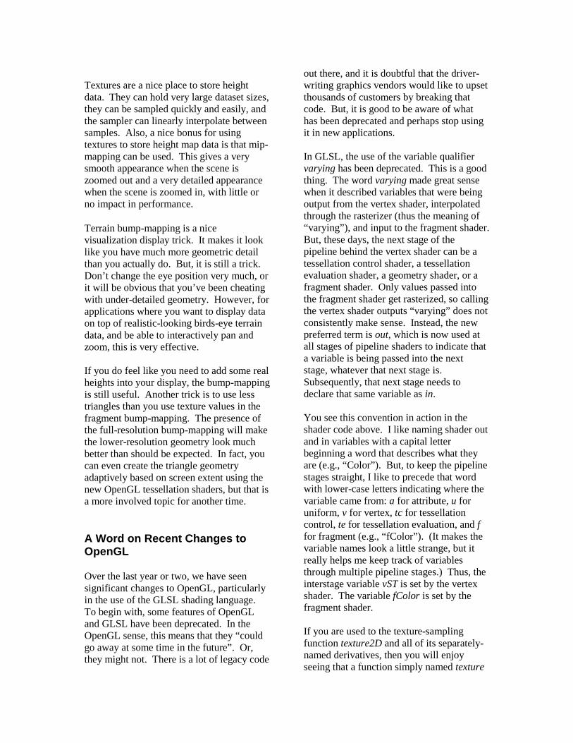
Textures are a nice place to store height data. They can hold very large dataset sizes, they can be sampled quickly and easily, and the sampler can linearly interpolate between samples. Also, a nice bonus for using textures to store height map data is that mip-mapping can be used. This gives a very smooth appearance when the scene is zoomed out and a very detailed appearance when the scene is zoomed in, with little or no impact in performance. Terrain bump-mapping is a nice visualization display trick. It makes it look like you have much more geometric detail than you actually do. But, it is still a trick. Don’t change the eye position very much, or it will be obvious that you’ve been cheating with under-detailed geometry. However, for applications where you want to display data on top of realistic-looking birds-eye terrain data, and be able to interactively pan and zoom, this is very effective. If you do feel like you need to add some real heights into your display, the bump-mapping is still useful. Another trick is to use less triangles than you use texture values in the fragment bump-mapping. The presence of the full-resolution bump-mapping will make the lower-resolution geometry look much better than should be expected. In fact, you can even create the triangle geometry adaptively based on screen extent using the new OpenGL tessellation shaders, but that is a more involved topic for another time. A Word on Recent Changes to OpenGL Over the last year or two, we have seen significant changes to OpenGL, particularly in the use of the GLSL shading language. To begin with, some features of OpenGL and GLSL have been deprecated. In the OpenGL sense, this means that they “could go away at some time in the future”. Or, they might not. There is a lot of legacy code

out there, and it is doubtful that the driver-writing graphics vendors would like to upset thousands of customers by breaking that code. But, it is good to be aware of what has been deprecated and perhaps stop using it in new applications. In GLSL, the use of the variable qualifier varying has been deprecated. This is a good thing. The word varying made great sense when it described variables that were being output from the vertex shader, interpolated through the rasterizer (thus the meaning of “varying”), and input to the fragment shader. But, these days, the next stage of the pipeline behind the vertex shader can be a tessellation control shader, a tessellation evaluation shader, a geometry shader, or a fragment shader. Only values passed into the fragment shader get rasterized, so calling the vertex shader outputs “varying” does not consistently make sense. Instead, the new preferred term is out, which is now used at all stages of pipeline shaders to indicate that a variable is being passed into the next stage, whatever that next stage is. Subsequently, that next stage needs to declare that same variable as in. You see this convention in action in the shader code above. I like naming shader out and in variables with a capital letter beginning a word that describes what they are (e.g., “Color”). But, to keep the pipeline stages straight, I like to precede that word with lower-case letters indicating where the variable came from: a for attribute, u for uniform, v for vertex, tc for tessellation control, te for tessellation evaluation, and f for fragment (e.g., “fColor”). (It makes the variable names look a little strange, but it really helps me keep track of variables through multiple pipeline stages.) Thus, the interstage variable vST is set by the vertex shader. The variable fColor is set by the fragment shader. If you are used to the texture-sampling function texture2D and all of its separately-named derivatives, then you will enjoy seeing that a function simply named texture

can now be used. It is an overloaded function, and its exact meaning depends on the type of sampler variable that is passed it. You will also notice a line at the top defining the GLSL version this code has been written against. By defining the version as 400, all the functionality in GLSL 4.00 will be available. If nothing is placed after the “400”, then this implies that you want to use the core functionality, and the compiler will whine if you use any features that have been deprecated. If instead you add the word compatibility to the #version line, then the compiler will let you get away with using all the deprecated features too. This way, you get to use everything. The vertex shader above uses the deprecated built-in variables gl_MultiTexCoord0 and gl_ModelViewProjectionMatrix, so it indicated that it wanted to be compiled in compatibility mode. The fragment shader, however, didn’t use any deprecated features, so it didn’t need to specify compatibility mode on the version line, although it would not have hurt. Those other two lines

precision highp float; precision highp int;

are there for OpenGL-ES compatibility. OpenGL-ES, the OpenGL API for embedded systems (i.e., mobile devices, etc.) wants the programmer to specify at what precision it should do variable arithmetic. This is so that it can save power if possible. You can specify the precision on a variable-by-variable basis, or, as shown here, specify precision for all variables of a particular type. OpenGL-desktop ignores these precision commands, but I have started adding them to all my new shader code anyway. Even though I’m not yet actively using OpenGL-ES (dabbling yes, seriously using no), I expect that soon I will be. When that happens, I would very much like to have all my shader code be compatible. In practice, your attitude towards OpenGL-ES migration

should have a large influence on how you use OpenGL-desktop now, and how quickly you abandon deprecated functionality. All educators who currently teach OpenGL-desktop need to think about this. If you are just teaching “graphics thinking”, then consider sticking with the compatibility mode. It will be around for a long time, maybe forever. It makes OpenGL programming easy to learn. If you are teaching serious graphics application development, you probably want to start migrating away from deprecated features and evolving to compatibility with OpenGL-ES. Acknowledgements Many thanks to NVIDIA and Intel for their continued support in this area. References Bailey2009 Mike Bailey, “Using GPU Shaders for Visualization”, IEEE Computer Graphics and Applications, Volume 29, Number 5, 2009, pp. 96-100.

Cabral1993 Cabral, Brian and Leith (Casey) Leedom, “Imaging Vector Fields Using Line Integral Convolution,” Computer Graphics (Proceedings of SIGGRAPH ’93), 1993, pp 263-270. CCoorrrriiee11999933 BBrriiaann CCoorrrriiee,, PPaauull MMaacckkeerrrraass.. ““DDaattaa SShhaaddeerrss,,”” PPrroocceeeeddiinnggss ooff IIEEEEEE VViissuuaalliizzaattiioonn 11999933,, pppp.. 227755--228822.. Knight1996 David Knight and Gordon Mallinson, "Visualizing Unstructured Flow Data Using Dual Stream Functions", Visualization and Computer Graphics, IEEE Computer Society, Vol 2, No 4, December 1996, pp 355-363. Lefohn2003 Aaron Lefohn, Joe Kniss, Charles Hansen, Ross Whitaker, “Interactive Deformation and Visualization of Level Set Surfaces Using Graphics Hardware”, Proceedings of IEEE Visualization 2003, pp. 75-82

Mark2003 William Mark, Steven Glanville, Kurt Akeley, and Mark Kilgard, “Cg: a system for programming graphics hardware in a C-like language,” Computer Graphics (Proceedings of SIGGRAPH 2003), pp. 896-907. McCormick2004 Patrick McCormick, Jess Inman, James Ahrens, Charles Hansen, Greg Roth, “Scout: A Hardware-Accelerated System for Quantitatively Driven Visualization and Analysis, Proceedings of IEEE Visualization 2004, pp. 171-179. International Workshop on Volume Graphics,, 2005, pp. 187-241. NED2010 http://ned.usgs.gov Petrovic2007 V. Petrovic, J. Fallon, F. Kuester, “Visualizing Whole-Brain DTI Tractography with GPU-based Tuboids and Level of Detail Management”, IEEE Transactions on Visualization and Computer Graphics, Volume 13, Number 6, Nov.-Dec. 2007, pp. 1488 – 1495. Scharsach 2005 H. Scharsach, “Advanced GPU raycasting”, Central European Seminar on Computer Graphics 2005, pp. 69-76. Sherbondy2003 Anthony Sherbondy, Mike Houston, Sandy Napel, “Fast Volume Segmentation with Simultaneous Visualization using Programmable Graphics Hardware”, Proceedings of IEEE Visualization2003, pp. 171-176.. Stegmaier2005 S. Stegmaier, M. Strengert, T. Klein, T. Ertl, “A simple and flexible volume rendering framework for graphics-hardware-based raycasting”. Fourth International Workshop on Volume Graphics, 2005, pp. 187-241.