using identical system synchronization with fractional

$: Using identical system synchronization with fractional$
Scientia Iranica B (2014) 21(6), 1920{1932

Sharif University of TechnologyScientia Iranica

Transactions B: Mechanical Engineeringwww.scientiairanica.com

Using identical system synchronization with fractionaladaptation law for identi�cation of a hyper-chaoticsystem

M. Abedini, M. Gomroki, H. Salarieh� and A. Meghdari

School of Mechanical Engineering, Sharif University of Technology, Tehran, P.O. Box 11155-9567, Iran.

Received 20 May 2013; received in revised form 25 January 2014; accepted 14 April 2014

KEYWORDSSystem identi�cation;Chaossynchronization;Fractional orderdynamics;L�u hyper-chaoticsystem;Adaptive control.

Abstract. Synchronization of two chaotic systems has been used in secure communica-tions. In this paper, synchronization of two identical 4D L�u hyper-chaotic systems is usedto identify the drive system. Parameters in both drive and response systems are unknownand the systems are synchronized by applying one state feedback controller. Since the goalhere is to identify the parameters of the drive system, an adaptive method is used. Thestability of the closed-loop system with the controller and convergence of parameters isstudied using the Lyapunov theorem. In order to improve the speed of convergence in oneparameter, a fractional adaptation law is used and the stability with the fractional law isshown. Finally, the results of both integer and fractional methods are compared.© 2014 Sharif University of Technology. All rights reserved.

1. Introduction

There is a phenomenon in nonlinear systems, whichis called chaos. Chaos also exists in many real worldproblems. The most signi�cant property of a chaoticsystem is high sensitivity to initial conditions. Itis important to see that two responses of a chaoticsystem with initial values very close to each otherdiverge exponentially but still stay in a boundedregion. This would cause some other properties ofchaotic systems, which have rich frequencies, and manyunstable periodic orbits. These properties of chaoticsystems make it di�cult to study them. The positiveLyapunov exponent is one way to show that a systemis chaotic. If the chaotic system has more than onepositive Lyapunov exponent, it would be called hyper-chaotic.

*. Corresponding author. Tel.: +98 21 66165586;Fax: +98 21 66000021E-mail addresses: [email protected] (M. Abedini);[email protected] (M. Gomroki); [email protected] (H.Salarieh); [email protected] (A. Meghdari)

In real world applications, parameters of a chaoticsystem may be particularly or fully unknown. So,identi�cation of the parameters of a chaotic systemhas been studied in many cases. Di�erent methodsare used for identi�cation, such as the neural networkstate space model [1], adaptive control [2], modi�edrecursive least square [3], robust control [4] etc. Mostof these methods use an adaptive law which comesfrom the Lyapunov-based stability proof for the closedloop system. In most cases, lack of information aboutthe system parameters makes it necessary to use anadaptation law. But, usually, these adaptation lawsmay not converge to true values and are just usedto estimate a value for the parameters. In somecases, when the chaotic system has fractional nonlineardi�erential equations, identi�cation has been madeusing optimization algorithms, such as Arti�cial NeuralNetworks (ANN) [5], Particle Swarm Optimization(PSO) [6], the output error approach [7] or di�erentialevolution [8].

Synchronization of chaotic systems was intro-duced for the �rst time in the research undertaken by

M. Abedini et al./Scientia Iranica, Transactions B: Mechanical Engineering 21 (2014) 1920{1932 1921

Pecora and Carroll [9] in 1990, and since then, it hasbeen an interesting topic for researchers [10-13]. Insynchronization of two systems, it is desired for theresponse system trajectories to follow the drive system.In many cases, parameters of the drive system areunknown, so, an adaptive method is used to estimatethe parameters [14-18]. So, synchronization of twoidentical systems can be used to identify the parametersof the drive system. Recently, there have been manymethods to synchronize two systems with unknownparameters. In [15,17], two non-identical chaoticsystems are synchronized by applying the adaptivecontrol law to each state of the response system. In [18],two identical chaotic systems are synchronized using acontrol law in only one of the states of the responsesystem. In [19], two identical L�u hyper-chaotic systemswith unknown parameters are synchronized with anadaptation law based on the Lyapunov stability theory.In [20], a new modi�ed hyper-chaotic L�u system issynchronized with the use of the adaptive control law.In [19,20], the controllers are applied to all states,but the parameters convergence to the correct valuesis not shown. And, �nally, in [21], two identical L�uhyper-chaotic systems with unknown parameters aresynchronized by applying one state controller. Basedon [21], in the present paper, some modi�cations areapplied in cases of parameter identi�cation in order toguarantee convergence to the correct values.

Fractional calculus has a history of about 300years and more recently been recognized in the workdone by Leibniz, Riemann, etc. Little attention waspaid to it at that time, but, recently, there have beenmany more applications using fractional calculus [8,22-24]. It has been used to model some systems, e.g.viscoelastic systems, suspension systems etc. [23].

Fractional calculus has recently stepped into thecontrol region and also chaos control [25-28]. Itis shown that using fractional order controllers canhave better results than using integer orders [29]. Indesigning a controller with fractional calculus, thereis one more parameter which gives the designers moredegrees of freedom to design a controller. This extraparameter is the order of di�erentiation that allowsgetting a better response from the controller, especiallyin the transient part of the solution.

In this paper a fractional order adaptation law isused to synchronize two integer order identical hyper-chaotic 4D L�u systems in order to identify the param-eters of the drive system. In other words, the mainidea here is to use chaos synchronization techniquesto synchronize virtual computer-based dynamics withunknown parameters as the \Response System", witha real dynamical chaotic system as the \Drive System".To achieve this, at �rst, the controller designed in [21]for synchronizing two 4D hyper-chaotic systems isdiscussed again here. Then, the parameters of the

response system are assumed to be unknown, and,using the Lyapunov stability theorem, an adaptivecontrol algorithm is designed. The important pointhere is to use fractional order dynamics in adaptationlaws to obtain better convergence and smaller oscilla-tions in parameter estimation. Finally, the stabilityof the system with fractional order is discussed andit is proved that the system with the fractional orderadaptation law remains stable.

2. Preliminaries and de�nitions

In fact, fractional calculus is a generalized version ofinteger order calculus. The integro-di�erential operatoris shown by t0 D�

t . Common formulations for fractionalderivatives are as follows.

De�nition 1. (Riemann-Liouville fractional deriva-tive [30]) The Riemann-Liouville fractional derivativeis de�ned as:

RLt0 D

�t f(t)=

8>>>><>>>>:1

�(��)

R tt0

(t��)��1f(�)d� � < 0

f(t) � = 0

Dn �t0D

��nt f(t)

�� > 0

(1)

where n � 1 � � < n and �(:) is the standard gammafunction, �(x) =

R10 tx�1e�tdt.

De�nition 2. (Caputo fractional derivative [30]) TheCaputo fractional derivative is de�ned as:

Ct0D

�t f(t)=

8<: 1�(n��)

R tt0

f(n)(�)(t��)�+1�n d� n� 1<�<n

Dnf(t) � = n (2)

The Caputo fractional derivative was almost used inengineering problems, because derivatives appeared oninteger points, so, they could have physical imple-mentation. But, in the Riemann-Liouville de�nition,derivatives appear in fractional points, and, in numer-ical solving, we must know the initial conditions inthe fractional points of derivation, which may have notphysical implementation.

De�nition 3. A dynamic system in fractional calculusis de�ned as:F�t; y(t);Ct0 D

�1t y(t);Ct0 D

�2t y(t); :::;Ct0 D

�nt y(t)

�=g(t);

(3)

where �1 < �2 < ::: < �n, F (t; y1; :::; yn) and g(t) arereal known functions. It can also be de�ned in the statespace form as:Ct0D

�it xi = fi (t; x1; x2; :::; xn) ;

xi(0) = Xi0; i = 1; 2; :::; n; (4)

where 0 < �i � 1 for i = 1; 2; :::; n.

1922 M. Abedini et al./Scientia Iranica, Transactions B: Mechanical Engineering 21 (2014) 1920{1932

A linear dynamic system in state space form islike:0BBB@

Ct0D

�1y x1

Ct0D

�2y x2...

Ct0D

�ny xn

1CCCA =

0BBB@a11 a12 � � � a1na21 a22 � � � a2n...

.... . .

...an1 an2 � � � ann

[email protected]

1CCCA= A

[email protected]

1CCCA : (5)

3. 4D L�u hyper-chaotic system

Systems with more than one (especially 2) positive Lya-punov exponents are known as hyper-chaotic systemsin literature. This implies that their dynamics areexpanded in several di�erent directions simultaneously.In recent years, several hyper-chaotic systems werediscovered in high-dimensional dynamics. For example,see the hyper-chaotic Rossler system [31], the hyper-chaotic Lorenz system [32], the hyper-chaotic Chuacircuit [33] etc.

The 4D L�u hyper-chaotic dynamical system isbased on the 3D original L�u system [34] by addinga state feedback. In 2006, Elabbasy, Agiza and El-Dessoky presented di�erential equations of the 4D L�uhyper-chaotic system as [19]:8>>>>>><>>>>>>:

_x1 = a(x2 � x1)

_x2 = cx2 � x1x3 + x4

_x3 = x1x2 � bx3

_x4 = x3 � dx4

(6)

in which, the 4th state is a simple state feedback whichis added to the 2nd state.

Both response and drive systems have character-istic equations, as the above, but the main di�erence isthat all the states of the response system are followedby a controller:8>>>>>><>>>>>>:

_y1 = a(y2 � y1) + u1

_y2 = cy2 � y1y3 + y4 + u2

_y3 = y1y2 � by3 + u3

_y4 = y3 � dy4 + u4

(7)

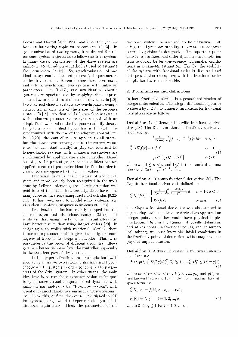
This system demonstrates a hyper-chaotic attractorwith many di�erent sets of parameters. In Fig-ure 1, trajectories of the 4D L�u system with a setof parameters (a = 20; b = 5; c = 10; d = 1:5)are shown. These parameters made the system to

Figure 1. Trajectories of the 4D L�u hyper-chaotic system.

be hyper-chaotic with Lyapunov exponents equal tof0:75; 0:03;�1:55;�15:73g.

The Lyapunov dimension of the system with theabove parameters is 3.34, which shows that the systemis hyper-chaotic.

3.1. SynchronizationIn [21], it was shown that the response system in Eq. (7)can be synchronized with the drive system in Eq. (6)using a single state feedback only on the 2nd state. Themain theorem is stated here.

Theorem 1. For Eq. (6), suppose that B2 andB3 are the upper bounds of absolute values of statevariables, x2 and x3, respectively. For the positiveconstant, � > dB2

2=a(4bd � 1) > 0, the system inEq. (7) with controllers u2 = �k2(y2 � x2), u1 = u3 =u4 = 0, can be synchronized to the system in Eq. (6),and the zero equilibrium point of the error dynamicsystem (e = y � x) is globally asymptotically stable,where:

k2 > max(g1; g2; g3);

g1 = min�

�(�a+B3)2

4�a+ c�> 0;

g2 = min�

�b(�a+B3)2

4�ab�B22

+ c�> 0;

g3 = min��

(�a+B3)2(4bd�1)+4�ab+2B2(�a+B3)�B22

4�a(4bd�1)�4dB22

+c�

> 0: (8)


Proof. The error dynamics can be easily obtained bysubtracting Eq. (6) from Eq. (7):8>>>>>><>>>>>>:

_e1 = a(e2 � e1) + u1

_e2 = ce2 + e4 � e1e3 � x1e3 � x3e1 + u2

_e3 = �be3 + e1e2 + x2e1 + x1e2 + u3

_e4 = e3 � de4 + u4

(9)

A Lyapunov function is de�ned here as:

V1(t) =12��e2

1 + e22 + e2

3 + e24�: (10)

Di�erentiating the Lyapunov function, with respect totime, yields:

_V1(t) =�e1 _e1 + e2 _e2 + e3 _e3 + e4 _e4

=�e1 (ae2 � ae1 + u1)

+ e2 (ce2 + e4 � e1e3 � x1e3 � x3e1)

+ e3 (�be3 + e1e2 + x2e1 + x1e2 + u3)

+ e4 (e3 � de4 + u4)

=� �ae21 + ce2

2 � be23

� de24 + e1e2 (�a� x3) + e2e4 + e3e4

+ e1e3(x2) + �e1u1 + e2u2 + e3u3 + e4u4:(11)

Substituting u1 = u3 = u4 = 0 and u2 = �k2e2 in theabove equation yields:

_V1(t) =� �ae21 + (c� k2)e2

2 � be23 � de2

4

+ e1e2(�a� x3) + e2e4 + e3e4 + e1e3(x2)

< �eTPe; (12)

where:

P =

0BBBBB@�a (��a+B3)

2�B2

2 0(��a+B3)

2 k2 � c 0 �12

�B22 0 b �1

2

0 �12

�12 d

1CCCCCA ;

e =

2666664je1jje2jje3jje4j

3777775 : (13)

In [21], it was shown that if all the above conditionsare satis�ed, matrix P would be positive de�nite, so,_V1(t) < 0, and the origin of the synchronization errorspace will be globally asymptotically stable. �3.2. Adaptive synchronizationIn real systems, some or all of the system parametersare unknown or maybe with some uncertainties. Theseunknown or uncertain parameters can completely de-stroy the procedure of synchronization. In this section,an adaptive synchronization method for two identicalhyper-chaotic L�u systems is developed.

Consider the response system stated in Eq. (7)again with estimated parameters, ar; br; cr and dr:8>>>>>><>>>>>>:

_y1 = ar(y2 � y1) + u1

_y2 = cry2 � y1y3 + y4 + u2

_y3 = y1y2 � bry3 + u3

_y4 = y3 � dry4 + u4

(14)

The response system is a computer-based system thatwe wish to synchronize with the real drive system inEq. (6), with unknown parameters.

The error dynamics equations can be derivedagain as:8>>>>>><>>>>>>:

_e1 = a(e2 � e1) + ea(y2 � y1) + u1

_e2 = ce2 + e4 + e1e3 � y1e3 � y3e1 + ecy2 + u2

_e3 = �be3 � e1e2 + y2e1 + y1e2 � eby3 + u3

_e4 = e3 � de4 � edy4 + u4

(15)

In the above equation, ea = ar � a is the parameterestimation error and eb; ec and ed are de�ned similarly.Now, we can de�ne the new Lyapunov function as:

V2(t)=V �1 (t) +12�e2a + e2

b + e2c + e2

d�+

12

(~k2 � k2)2;(16)

where ~k2 is the estimate of the controller gain and V �1 (t)is in the form of Eq. (10). _V �1 (t) is computed as:

_V �1 (t) =�e1 _e1 + e2 _e2 + e3 _e3 + e4 _e4

=�e1 (ae2 � ae1 + eay2 � eay1 + u1)

+ e2 (ce2+e4+e1e3�y1e3�y3e1+ecy2+u2)

+ e3 (�be3�e1e2+y2e1+y1e2 � eby3+u3)

+ e4 (e3 � de4 � edy4 + u4) : (17)

Then, here the rate of change vs. time of the Lyapunovfunction is:


_V2(t) = _V �1 (t) + ea _ea + eb _eb + ec _ec + ed _ed

+ (~k2 � k2) _~k2: (18)

Assuming again u1 = u3 = u4 = 0 and u2 = �~k2e2,the above equation can be expanded as:

_V2(t) =� �ae21 + (c� k2)e2

2 � be23 � de2

4

+ e1e2(�a� x3) + e2e4 + e3e4 + e1e3(x2)

+ ea(�e1y2 � �e1y1 + _ea) + ec(y2e2 + _ec)

+ eb(�e3y3 + _eb) + ed(�y4e4 + _ed)

+ (~k2 � k2)( _~k2 � e22): (19)

Thus:

_V2(t) = _V1(t) + ea(�e1y2 � �e1y1 + _ea)

+ ec(y2e2 + _ec) + eb(�e3y3 + _eb)

+ ed(�y4e4 + _ed) + (~k2 � k2)( _~k2 � e22); (20)

where _V1(t) < �eTPe, as shown in Eq. (12). Bysubstituting the adaptation laws as:

_ea = ��e1y2 + �e1y1;

_eb = y3e3;

_ec = �y2e2;

_ed = y4e4;

_~k2 = e22; (21)

and applying in Eq. (20), we have:

_V2(t) = _V1(t) < �eTPe) _V2(t) � 0: (22)

Lemma 1. Consider all assumptions in Theorem 1.The zero equilibrium point of the error dynamic systemin Eq. (15) is globally asymptotically stable by applyingadaptation laws in Eq. (21) and using controller, u2 =�~k(y2 � x2), u1 = u3 = u4 = 0.

Proof. P is a symmetric positive de�nite matrix, so,it can be written in the form:

P = STS: (23)

So, we have:

_V2(t) � �(Se)T (Se); (24)

where S is a constant nonsingular matrix.

Assume the integral below:

I =Z 1

0� _V2(t)dt = V2(0)� V2(1): (25)

Since _V2 is negative and V2(t) is always positive, V2(1)is bounded; it means that integral I is bounded too.According to Relation (24):Z 1

0(Se)T (Se)dt < I: (26)

So, one can say:

(Se) 2 L2: (27)

Again, since _V2 is negative semi de�nite, all of thestate errors and parameter estimation errors will bebounded. Consequently, the time derivative of errorsin Eq. (15) will be bounded and d(Se)

dt = S _e will bebounded too.

Now, using the Barbalat lemma, we may have:

limt!1Se(t) = 0: (28)

According to the fact that S is nonsingular, it can besaid:

limt!1e(t) = 0: (29)

So, the proof is completed. �Now, if we solve equation _V2 = 0 according

to Lemma 1, the only admissible answer, when timeconverges to in�nity, is the inevitable solution, whichis e(1) = 0. Applying this solution to the system inEq. (15) and knowing that _e(1) = 0, we will have:

ea(1) = eb(1) = ec(1) = ed(1) = 0: (30)

So, using LaSalle's invariant principle [35], the originof the system of Eqs. (15) and (21), together, will beasymptotically stable.

The above statements can be collected in thefollowing theorem.

Theorem 2. Consider all assumptions in Theorem 1.Eq. (7) with controllers u1 = u3 = u4 = 0 and u2 =�~k(y2�x2) can be synchronized to Eq. (6), and the zeroequilibrium point of error dynamic system in Eq. (15) isglobally asymptotically stable by applying adaptationlaws in Eq. (21), and the convergence of the parametersis guaranteed.

Proof. The whole procedure is stated from thebeginning of the current subsection. �

According to Theorem 2, a computer-based sys-tem in Eq. (14) with unknown parameters, ar; br; crand dr, can be synchronized with the real system inEq. (6) by measuring all the states and using a singlestate feedback only. Theorem 2 shows that the errorsgo to zero asymptotically and the parameters alsoconverge to true values.


4. Chen chaotic system

In this section, we take Chen chaotic system as ourdrive system. Its di�erential equations are [36]:8>>><>>>:

_x1 = a(x2 � x1)

_x2 = bx2 � cx1 � x1x3

_x3 = x1x2 � dx3

(31)

where the parameters are a = 35, b = 28, c = 7 andd = 3. Also, we take the response system to be thesame as the drive one.8>>><>>>:

_y1 = a(y2 � y1) + u1

_y2 = by2 � cy1 � y1y3 + u2

_y3 = y1y2 � dy3 + u3

(32)

4.1. SynchronizationTheorem 3. For system in Eq. (31), as in Theorem 1,suppose that B2 and B3 are the upper bounds ofabsolute values of state variables, x2 and x3, respec-tively. For the positive constant, � > B2

2=4ad > 0,Eq. (32) with controllers, u2 = �k2(y2 � x2) andu1 = u3 = 0, can be synchronized to Eq. (31) andthe zero equilibrium point of error dynamic system(e = y � x) is globally asymptotically stable, where:

k2 > max(g1; g2);

g1 = min�

�(�a� c+B3)2

4�a+ b�> 0;

g2 = min�

�d(�a� c+B3)2

4�ad�B22

+ b�> 0: (33)

Proof. The procedure is completely like the proof oftheorem 1. �4.2. Adaptive synchronizationConsider the response system stated in Eq. (32) again,with estimated parameters, ar; br; cr and dr:8>>><>>>:

_y1 = ar(y2 � y1) + u1

_y2 = bry2 � cry1 � y1y3 + u2

_y3 = y1y2 � dry3 + u3

(34)

Theorem 4. Consider all assumptions in Theorem 3.The system in Eq. (32) with controllers u1 = u3 = 0and u2 = �~k(y2�x2) can be synchronized to Eq. (31),and the zero equilibrium point of error dynamic systemis globally asymptotically stable by applying adapta-tion laws in Eq. (35). Thus, the convergence of theparameters is guaranteed.

_ea = ��e1y2 + �e1y1;

_eb = �y2e2;

_ec = y1e2;

_ed = y3e3;

_~k2 = e22: (35)

Proof. The whole procedure is completely like theproof of Theorem 2. �

5. Fractional adaptation

The 4D L�u system is hyper-chaotic; therefore the speedof parameter identi�cation is very important in syn-chronization. So, we can change the adaptation laws'dynamics with fractional order equations to obtainbetter identi�cation and faster state synchronization.

To achieve this goal, adaptation laws are assumedto be:

D�1ea = ��e1y2 + �e1y1;

D�3eb = y3e3;

D�2ec = �y2e2;

D�4ed = y4e4; (36)

where 0 < �i � 1 and D� denotes the Caputoderivative from t0 = 0. Because of the similarity offractional systems with a derivative order of less thanone to damped systems, these new adaptation lawswould be stable and can estimate parameters faster andwith fewer uctuations.

Also, here, for achieving better convergence insingle-state feedback gain, the dynamics of controllergain can be assumed to be fractional as:

D�~k2 = e22; (37)

where 0 < � � 1 too.As we will see in the next section, convergence

in parameters a; b and c are faster than d and itseems to be over-damped. But, parameter d has some uctuations, and, then, error in the 4th state takesmore time to go to zero. This problem can be solvedeasily by applying less degrees of di�erentiation in theadaptation law for this parameter.

Also for the Chen chaotic system, we take thefollowing as adaptation laws:

D�1ea = ��e1y2 + �e1y1;

D�2eb = �y2e2;

D�3ec = y1e2;

D�4ed = y3e3;

D�5 ~k2 = e22; (38)


in which we use �4 = 0:7 for parameter d, and otheradaptation laws remain in integer order.

6. Numerical simulations

In this section, numerical simulations are pre-sented to show the e�ectiveness of the fractionalmethod discussed in the previous section. ThePECE algorithm [37] is used to solve di�erentialEqs. (6), (14), (36) and (37), assuming a Caputoderivative with a time step of size 0.001. This methodis like fourth-order Runge-Kutta for integer orderequations. For fractional solution only, in Eq. (36),�4 = 0:55 is taken and all others are equal to 1, whichmeans they are integer order di�erential equations.B2 = B3 = 20 and � = 2:0345 are taken, and tosolve Eq. (6), the parameters are taken as a = 20; b =5; c = 10; d = 1:5 and the initial conditions are setas x0 =

�0:1; 0:1; 0:1; 0:1

�T . Also, the initialconditions for Eqs. (14), (36) and (37) are, respectively,y0 =

��9:9; �4:9; 5:1; 10:1�T , ar(0) = 25, br(0) =

10, cr(0) = 15, dr(0) = 6 and ~k2(0) = 30.Figure 2 shows the estimation of parameters

for ar; br; cr, and Figure 3 shows the estimation ofparameter dr of the 4D L�u hyper-chaotic system. Itis obvious that all of them are converged to their truevalue by both methods. But, according to these two

Figure 2. Three parameter estimation ar, br and cr forthe 4D L�u hyper-chaotic system.

Figure 3. Parameter estimation dr for the 4D L�uhyper-chaotic system.

�gures, parameter dr uctuates more than others inthe integer order method. So, the fractional ordermethod is used for modifying the equation of thisparameter and dr converges smoothly to the �nalvalue. This method almost does not a�ect the otherestimations. Also, Figure 4 shows the convergency ofthe last parameter when a di�erent order of fractionalderivative is used.

Figure 5 shows the error of synchronization forthe �rst, second and third state of the response systemand Figure 6 shows the error of synchronization forthe fourth state of the 4D L�u hyper-chaotic system. Itshows that the di�erence between the fractional andinteger order method is negligible for the �rst threestates. Also, these three errors approach zero fast and

Figure 4. Error in parameter estimation dr with di�erentfractional orders for the 4D L�u hyper-chaotic system.

Figure 5. Synchronization error of the �rst three statesfor the 4D L�u hyper-chaotic system.

Figure 6. Synchronization error of the fourth state forthe 4D L�u hyper-chaotic system.


Figure 7. Control gain calculation for the 4D L�uhyper-chaotic system.

Figure 8. Three parameter estimation ar, br and cr forthe Chen chaotic system.

almost in a proper manner in comparison to the laststate in the integer method. The reason why the laststate error uctuates is because parameter dr uctuatesin this method of solution. But, the fractional methodcauses both estimations and, consequently, synchro-nization error would converge more smoothly.

Figure 7 shows the control gain estimation forboth integer order and fractional order methods for the4D L�u hyper-chaotic system.

In numerical simulation of the Chen chaotic sys-tem, in Eq. (38), �4 = 0:7 is taken and all othersare equal to 1, which means they are integer orderdi�erential equations. B2 = 30, B3 = 50 and � =3 are taken, and to solve Eq. (31), the parametersare assumed as a = 35; b = 28; c = 7; d = 3 andthe initial conditions are set to x0 =

�1; 5; 20

�T .Also, the initial conditions for Eqs. (34) and (38) are,respectively, y0 =

��7; �10; 35�T , ar(0) = 30,

br(0) = 32, cr(0) = 3, dr(0) = 7 and ~k2(0) = 211.Figure 8 shows the estimation of parameters

for ar; br; cr and Figure 9 shows the estimation ofparameter dr of the Chen chaotic system. As seen,all parameters have converged to their actual value.Also, the estimation of dr has less uctuations in thefractional order method and has settled sooner. Actu-ally, settling time using the fractional order methodis almost one third of the integer order method.

Figure 9. Parameter estimation dr for the Chen chaoticsystem.

Figure 10. Error in parameters estimation ar, br and crwith di�erent fractional orders for the Chen chaoticsystem.

Figure 11. Synchronization error of the �rst and secondstates for the Chen chaotic system.

Moreover, the fractional order method does not a�ectother estimations.

In Figure 10, estimation of parameters ar, br andcr for the Chen chaotic system is shown. The di�erenceis that for each parameter, one of the adaptation lawsin Eq. (38) is obtained as fractional to examine thee�ect of fractional order in other parameters. As can beseen, while �i is getting closer to unity, the estimationbecomes better.

Figures 11 and 12 show synchronization errorsfor the states of the Chen chaotic system. In both


Figure 12. Synchronization error of the third state forthe Chen chaotic system.

Figure 13. Control gain calculation for the Chen chaoticsystem.

responses, the error has become zero, but, in thefractional order, according to the in uence of dr onthe third state, it has settled sooner with fewer uctua-tions. Also, it is obvious in Figure 11 that the fractionalorder method does not a�ect the response.

Figure 13 shows the control gain estimation forboth integer order and fractional order methods for theChen chaotic system.

7. Stability analysis

As mentioned in the previous section, the adaptationlaw for parameter d is replaced by the following:

D�ed = y4e4; (39)

where D� denotes the Caputo derivative with t0 = 0.The Caputo derivative de�nition plays an importantrole in stability analysis because they have appeared in-side the integral (see Eq. (2)) and we used this property.All other adaptation laws were kept unchanged. Wecan now rearrange the Lyapunov function in Eq. (20)as the following:

_V2(t) = _V1(t) + ea (�e1y2 � �e1y1 + _ea)

+ ec(y2e2 + _ec) + eb(�e3y3 + _eb)

+ (~k2 � k2)( _~k2 � e22) + ed(�y4e4

+D�ed �D�ed+ _ed) = :::

+ ed(�y4e4+D�ed)+ed( _ed�D�ed): (40)

Substituting adaptation laws in the above equation

yields:

_V2(t) = _V1(t) + ed( _ed �D�ed) < �eTPe

+ ed( _ed �D�ed): (41)

It is enough to show that the last term is negativeand/or behaves in an appropriate manner.

Lemma 2. Consider:

w(�) =1

�(1� �)(t� �)�� 1

�(1� �)(t� �)�;

where 0 < � < � < 1. Function w(�) is always negativeand descending when t > 0, 0 � � � t and � ! 1.

Proof. We can rewrite w(�) as:

w(�) =�(1� �)(t� �)� � �(1� �)(t� �)�

�(1� �)(t� �)��(1� �)(t� �)�: (42)

The denominator of w(�) is always positive, so, wemust prove only that the numerator is negative. Let usde�ne n(�) as:

n(�) ,num (w(�)) = �(1� �)(t� �)�

� �(1� �)(t� �)� ) n(0) = �(1� �)t�

� �(1� �)t� : (43)

It is obvious that for any positive t there exists a � near1 where n(0) is negative. Besides, we have:

lim�!1t>0

n(0) = lim�!1t>0

�(1� �)t� � �(1� �)t� = �1

) lim�!1t>0

w(0) < 0:(44)

Again, computing a derivative of n(�) with respect to� , we have:

dd�n(�)=�(1� �)�(t� �)��1��(1� �)�(t� �)��1;

(45)

which is negative when 0 � � � t and � is near 1. Now,we want to �nd the zero point of the above functionwith respect to � :

dd�n(�) = 0

) �(1� �)�(t� �)��1 = �(1� �)�(t� �)��1

) �(1� �)��(1� �)�

= (t� �)��

) �� = t��

�(1� �)��(1� �)�

�1=��: (46)


We can easily show �� ! t, when � ! 1, so, dd� n(�)

has no zero point in the interval (0; t). From Eqs. (42)to (46), we see:1. w(�) is a function with a negative starting point.

w(0) < 0;2. The denominator of w(�) is always positive and

ascending; numerator n(�) has a negative derivativein all domains (0; t).

So, w(�) is a negative and descending function allover the domain. �

Proposition. The term ed( _ed � D�ed) in Eq. (41)always behaves such that the asymptotic stability ofthe controlled system is guaranteed.

Discussion. Let us replace _ed with D�ed, where � istending to 1. So, we may have:

ed(0D�t ed �0 D�

t ed) = ed(t)

��

1�(1� �)

Z t

0

_ed(�)d�(t� �)�

� 1�(1� �)

Z t

0

_ed(�)d�(t� �)�

�= ed(t)

�Z t

0_ed(�)d�

�1

�(1� �)(t� �)�

� 1�(1� �)(t� �)�

��: (47)

De�ning:

w(�) =1

�(1� �)(t� �)�� 1

�(1� �)(t� �)�;

we have:

ed(0D�t ed �0 D�

t ed) = ed(t)Z t

0w(�) _ed(�)d�; (48)

where w(�) is a weight function. From Lemma 2, wehave seen w(�) is always a negative descending functionwhen � ! 1. We de�ne Ai and Ii as below:

Ii =Z �i

�i�1

Ai(t; �)w(�)d�; i = 1; :::; N

Ai(� 0; �) = ed(� 0) _ed(�); � 2 [�i�1; �i]; (49)

where �0 = 0 and �N = t. Also, the sign of Ai(�; �) doesnot change in interval [�i�1; �i], so, N is the number ofchanging signs occurred in Ai(�; �) before both ed and_ed tend to zero. Now, Eq. (48) can be rewritten againas:I = ed( _ed �D�ed)

= ed(t)Z t

0w(�) _ed(�)d� =

NXi=1

Ii: (50)

ed and _ed are continuous, and only one of ed(t) or _ed(t)changes signs when A(�; �) changes sign.

Proposition. Consider the sign of Ai(�; �) in interval[�i�1; �i]:

� If it has a positive sign, it means that ed and _ed havethe same sign and the system goes to instability.So, at the end of the interval at � = �i only _ed canchange sign.

� If it has a negative sign, it means ed and _ed have theopposite sign. So, ed tends to zero and changes signat the end of the interval at � = �i.

Now, we discuss the number of intervals, N :

- If N = 1, it is clear that I = I1 and no change insign of ed or _ed is occurred.

I = I1 = ed(t)�Z t

0_ed(�)w(�)d�

�=Z t

0ed(t) _ed(�)w(�)d�

=Z t

0A1(t; �)w(�)d; �

if A1(t; �) > 0) I < 0) _V2(t) <�eTPe + I<0

if A1(t; �) < 0;

)8<:if eTPe > I) _V2(t) < 0

if eTPe < I) eTPe is bounded(51)

It is obvious that if ed and _ed have opposite signs, jedjtends to zero, so, the upper bound of eTPe tends tozero and the system is stable.- If N = 2, it is clear that I = I1 + I2 and only onechange in sign of ed or _ed is occurred.

I. Assume A1(�; �) < 0, so A2(�; �) > 0. Fromthe previous proposition, we know the sign of _ed(�)cannot change at � = �1, then, the sign of ed(�) ischanged at � = �1. For t < �1, A1(t; �) < 0 is alwaysnegative, so, ed(�) tends to zero at the end of thisinterval. At the second interval, when �1 < t < �2,we may have:

for t > �1 : _V2(t) < �eTPe + I1 + I2 = �eTPe

+Z �1

0A1(t; �)w(�)d�+

Z �2

�1A2(t; �)w(�)d�

8t < �1 : A1(t; �) < 0

) 8t > �1 : A1(t; �) > 08t > �1 : A2(t; �) > 0

�) I1; I2 < 0) _V2(t) < 0: (52)

II. Assume A1(�; �) > 0, so, A2(�; �) < 0. From


the previous proposition, we know the sign of _ed(�)changes at � = �1. In the �rst interval, we have:

for t < �1 : _V2(t) < �eTPe + I1 = �eTPe

+Z �1

0A1(t; �)w(�)d� < 0: (53)

So, the system is stable. In the second interval:

for t > �1 : _V2(t) < �eTPe + I1 + I2 = �eTPe

+Z �1

0A1(t; �)w(�)d� +

Z �2

�1A2(t; �)w(�)d�

8 t < �1 : A1(t; �) > 0

) 8 t > �1 : A1(t; �) > 0

8 t > �1 : A2(t; �) < 0

)) I1 < 0; I2 > 0 (54)

We can rewrite Eq. (54) like Eq. (51) and then:8>>>><>>>>:if eTPe� I1 > I2 ) _V2(t) < 0

if eTPe� I1 < I2 ) eTPe < I2

) eTPe is bounded

(55)

Again, it is obvious that if ed and _ed have oppositesigns, jedj tends to zero, so, the upper bound of eTPetends to zero and the system is stable.

This analysis can be repeated for N � 3. �

8. Conclusions

This paper has shown that identi�cation of chaoticor hyper-chaotic systems can be done based on thesynchronization of two identical systems. Two sys-tems are synchronized by applying one state feedbackcontroller. Adaptation laws used to �nd unknownparameters came from the Lyapunov stability theorem.By applying fewer degrees of di�erentiation in someof the adaptation laws (usually parameters with moreripples), less uctuations in convergence of the param-eter occur, as the results have shown in the numericalsimulations. Finally, a discussion about the analyticalproof of the stability of the controlled system using thefractional adaptation law is presented.

As can be seen, all simulations and analyseshave been undertaken assuming Caputo de�nition forfractional di�erentiation. In the Riemann- Liouvillede�nition, di�erentiation takes place after integration,so, some analyses and discussions may be done forother types of fractional-order derivatives in futurework.

References

1. Suykens, J.A., De Moor, B.L.R. and Vandewalle, J.\Nonlinear system identi�cation using neural statespace models, applicable to robust control design",International Journal of Control, 62(1), pp. 129-152(1995).

2. Ge, Z.M. and Leu, W.Y. \Chaos synchronizationand parameter identi�cation for loudspeaker systems",Chaos, Solitons and Fractals, 21(5), pp. 1231-1247(2004).

3. Motallebzadeh, F., Jahed Motlagh, M.R. and Rah-mani Cherati, Z. \Synchronization of di�erent-orderchaotic systems: Adaptive active vs. optimal control",Communications in Nonlinear Science and NumericalSimulation, 17(9), pp. 3643-3657 (2012).

4. Shen, L. and Wang, M. \Robust synchronization andparameter identi�cation on a class of uncertain chaoticsystems", Chaos, Solitons and Fractals, 38(1), pp. 106-111 (2008).

5. Al-Assaf, Y., El-Khazali, R. and Ahmad, W. \Iden-ti�cation of fractional chaotic system parameters",Chaos, Solitons and Fractals, 22(4), pp. 897-905(2004).

6. Yuan, L.-G. and Yang, Q.-G. \Parameter identi�ca-tion and synchronization of fractional-order chaoticsystems", Communications in Nonlinear Science andNumerical Simulation, 17(1), pp. 305-316 (2012).

7. Sabatier, J., Aoun, M., Oustaloup, A., Gr�egoire, G.,Ragot, F. and Roy, P. \Fractional system identi�cationfor lead acid battery state of charge estimation", SignalProcessing, 86(10), pp. 2645-2657 (2006).

8. Tang, Y., Zhang, X., Hua, C., Li, L. and Yang, Y.\Parameter identi�cation of commensurate fractional-order chaotic system via di�erential evolution",Physics Letters A, 376(4), pp. 457-464 (2012).

9. Pecora, L.M. and Carroll, T.L. \Synchronization inchaotic systems", Physical Review Letters, 64(8), pp.821-824 (1990).

10. Zhou, A., Ren, G., Shao, C. and Liang, Y. \Synchro-nization of chaotic system with uncertain functions andunknown parameters using adaptive poles method",Procedia Engineering, 29(0), pp. 2453-2457 (2012).

11. Wang, B., Wen, G. and Xie, K. \On the synchro-nization of a hyperchaotic system based on adaptivemethod", Physics Letters A, 372(17), pp. 3015-3020(2008).

12. Wang, B. and Wen, G. \On the synchronization ofa class of chaotic systems based on backsteppingmethod", Physics Letters A, 370(1), pp. 35-39 (2007).

13. Pourmahmood, M., Khanmohammadi, S. and Al-izadeh, G. \Synchronization of two di�erent uncertainchaotic systems with unknown parameters using arobust adaptive sliding mode controller", Communica-tions in Nonlinear Science and Numerical Simulation,16(7), pp. 2853-2868 (2011).


14. Chen, S. and L�u, J. \Parameters identi�cation andsynchronization of chaotic systems based upon adap-tive control", Physics Letters A, 299(4), pp. 353-358(2002).

15. Huang, L., Wang, M. and Feng, R. \Parametersidenti�cation and adaptive synchronization of chaoticsystems with unknown parameters", Physics LettersA, 342(4), pp. 299-304 (2005).

16. Yan, J.-J., Hung, M.-L., Chiang, T.-Y. and Yang,Y.-S. \Robust synchronization of chaotic systems viaadaptive sliding mode control", Physics Letters A,356(3), pp. 220-225 (2006).

17. Wu, Y., Zhou, X., Chen, J. and Hui, B. \Chaossynchronization of a new 3D chaotic system", Chaos,Solitons and Fractals, 42(3), pp. 1812-1819 (2009).

18. Yu, W. \Synchronization of three dimensional chaoticsystems via a single state feedback", Communica-tions in Nonlinear Science and Numerical Simulation,16(7), pp. 2880-2886 (2011).

19. Elabbasy, E.M., Agiza, H.N. and El-Dessoky, M.M.\Adaptive synchronization of a hyperchaotic systemwith uncertain parameter", Chaos, Solitons and Frac-tals, 30(5), pp. 1133-1142 (2006).

20. Zhou, X., Wu, Y., Li, Y. and Xue, H. \Adaptivecontrol and synchronization of a new modi�ed hyper-chaotic L�u system with uncertain parameters", Chaos,Solitons and Fractals, 39(5), pp. 2477-2483 (2009).

21. Yang, C.-C. \Adaptive synchronization of L�u hyper-chaotic system with uncertain parameters based onsingle-input controller", Nonlinear Dynamics, 63(3),pp. 447-454 (2011).

22. Zhu, H., Zhou, S. and Zhang, J. \Chaos and synchro-nization of the fractional-order Chua's system", Chaos,Solitons and Fractals, 39(4), pp. 1595-1603 (2009).

23. Matouk, A.E. \Chaos, feedback control and synchro-nization of a fractional-order modi�ed AutonomousVan der Pol-Du�ng circuit", Communications in Non-linear Science and Numerical Simulation, 16(2), pp.975-986 (2011).

24. Hegazi, A.S. and Matouk, A.E. \Dynamical behaviorsand synchronization in the fractional order hyper-chaotic Chen system", Applied Mathematics Letters,24(11), pp. 1938-1944 (2011).

25. C�elik, V. and Demir, Y. \E�ects on the chaoticsystem of fractional order PI� controller", NonlinearDynamics, 59(1-2), pp. 143-159 (2010).

26. Sadeghian, H., Salarieh, H., Alasty, A. and Meghdari,A. \On the control of chaos via fractional delayedfeedback method", Computers and Mathematics withApplications, 62(3), pp. 1482-1491 (2011).

27. Tavazoei, M.S., Haeri, M. and Jafari, S. \Taming sin-gle input chaotic systems by fractional di�erentiator-based controller: Theoretical and experimental study",Circuits, Systems, and Signal Processing, 28(5), pp.625-647 (2009).

28. Tavazoei, M.S., Haeri, M., Bolouki, S. and Siami,M. \Using fractional-order integrator to control chaosin single-input chaotic systems", Nonlinear Dynamics,55(1-2), pp. 179-190 (2009).

29. Tavazoei, M.S., Haeri, M. and Jafari, S. \Fractionalcontroller to stabilize �xed points of uncertain chaoticsystems: Theoretical and experimental study", Pro-ceedings of the Institution of Mechanical Engineers.Part I: Journal of Systems and Control Engineering,222(3), pp. 175-184 (2008).

30. Podlubny, I., Fractional Di�erential Equations: AnIntroduction to Fractional Derivatives, Fractional Dif-ferential Equations, to Methods of Their Solution andSome of Their Applications, Academic Press (1999).

31. Al-Sawalha, M.M. and Noorani, M.S.M. \Applicationof the di�erential transformation method for the solu-tion of the hyperchaotic R�ossler system", Communica-tions in Nonlinear Science and Numerical Simulation,14(4), pp. 1509-1514 (2009).

32. Mahmoud, E.E. \Dynamics and synchronization ofnew hyperchaotic complex Lorenz system", Mathemat-ical and Computer Modelling, 55(7-8), pp. 1951-1962(2012).

33. Thamilmaran, K., Lakshmanan, M. and Venkatesan,A. \Hyperchaos in a modi�ed canonical Chua's cir-cuit", International Journal of Bifurcation and Chaosin Applied Sciences and Engineering, 14(1), pp. 221-243 (2004).

34. Wang, G., Zhang, X., Zheng, Y. and Li, Y. \Anew modi�ed hyperchaotic L�u system", Physica A:Statistical Mechanics and Its Applications, 371(2), pp.260-272 (2006).

35. Khalil, H.K., Nonlinear Systems, Prentice Hall (2002).

36. Chen, G. and Ueta, T. \Yet another chaotic attrac-tor", International Journal of Bifurcation and Chaos,09(07), pp. 1465-1466 (1999).

37. Diethelm, K., Ford, N.J., Freed, A.D. and Luchko, Y.\Algorithms for the fractional calculus: A selectionof numerical methods", Computer Methods in AppliedMechanics and Engineering, 194(6-8), pp. 743-773(2005).

Biographies

Mohammad Abedini was born in 1986. He receivedhis BS and MS degrees in Mechanical Engineering in2006 and 2008, respectively, from Sharif University ofTechnology, Tehran, Iran, where he is currently a PhDdegree student of Mechanical Engineering and memberof the Center of Excellence in Design, Robotics andAutomation (CEDRA). His research interests includenonlinear dynamics and chaos, control, automation androbotics, mechatronics and real-time programming.

Mehdi Gomroki obtained BS and MS degrees in Me-chanical Engineering from Sharif University of Technol-


ogy, Tehran, Iran, in 2011 and 2013, respectively. Hisresearch interests include control, chaotic dynamics,chaos synchronization and fractional order calculations.

Hassan Salarieh received BS, MS and PhD degreesin Mechanical Engineering in 2002, 2004 and 2008,respectively, from Sharif University of Technology,Tehran, Iran, where he is currently Associate Professor.His research interests include chaos control, analysisof chaotic systems and fractional systems analysis andcontrol.

Ali Meghdari received his PhD degree in MechanicalEngineering from the University of New Mexico in1987, and joined the Los Alamos National Laboratoryas a Research Scientist for one full year. He is cur-rently Full-Professor of Mechanical Engineering, Vice-

President of Academic A�airs, and Director of the Cen-ter of Excellence in Design, Robotics and Automation(CEDRA) at Sharif University of Technology, Tehran,Iran.

Dr Meghdari has performed extensive research inthe areas of robotics dynamics, exible manipulatorskinematics/dynamics, and dynamic modeling of biome-chanical systems.

He has published over 160 technical papers inrefereed international journals and conferences, andhas been the recipient of various scholarships andawards, the latest being the 2002 Mechanical En-gineering Distinguished Professorship Award by theIranian Ministry of Science, Research and Technology.He was also nominated and elected Fellow of theASME (American Society of Mechanical Engineers) in2001.

using identical system synchronization with fractional

Documents