Using MatlabECE 303: Introduction to Communication Principles

Fall 2010

I. WHAT IS MATLAB?

Matlab is an interactive, matrix-based programming tool with high-level computational power for technical computing.Matlab has hundreds of functions in the mail toolbox as well as in several other toolboxes that are application specific. Theprogramming in Matlab is very simple because most of the Matlab programs can be written by calling the existing functions.

Typical uses include but are not limited to:• Math and computation• Algorithm development• Modeling, simulation, and prototyping• Data analysis, exploration, and visualization• Scientific and engineering graphics• Application development, including graphical user interface building

II. STARTING MATLAB

On your PC click on the Matlab icon as a shortcut on the Desktop or in the Start menu. After loading, you should seesomething like this screen.

The main windows consist of:1) Workspace: Contains variables that have been created in the Command Window or Editor. You can view any variable in

the Workspace by double-clicking it. You can clear the general variable ‘XXX’ by entering clear XXX in the CommandWindow. All variables can be cleared from the workspace by entering clear all in the Command Window.

2) Editor: A built-in text editor allowing you to enter the commands of your program. Commands are executed sequentiallyfrom top to bottom.

3) Command Window: Allows you to enter commands one at a time by entering the statement and hitting enter. TheCommand Window can be cleared by entering clc into the Command Window.

If you don’t find any of these windows open when loading Matlab, they can be found in the ‘Desktop’ tab at the top. Forexample click Desktop→ Editor to open the Editor window. Scripts generated in the Editor are known as M-files and have tobe saved with a .m extension, e.g. filename.m. Matlab must be steered to the same directory as the script for the program torun. The directory (shown by Current Directory: at the top) can be changed by clicking the button shown by an arrow in the

above figure and navigating to the directory where the M-file is saved. To run the script, click the button with a green arrowat the top of the Editor window.

III. VECTORS AND MATRICES

Creating vectors and matrices in Matlab is one of the easiest yet most fundamental parts of programming in this language.When creating a vector or matrix valued variable, spaces or commas (,) always delineate a new column, semicolons (;) alwaysdelineate rows, and the first and last entry in the matrix must be closed with square brackets ([ and ], respectively). To createa 1× 3 row-vector enter the following command

Likewise a 3× 1 column vector

The following command creates a 3× 3 square matrix

To reference an element in an array, type the name of the variable along with (row,col). For example, the following commandfinds the element in the second row and third column

To reference more than one element, do the same but with (row1:row2,col1:col2). For example, if we want rows 1 through 2and columns 2 through 3 we type

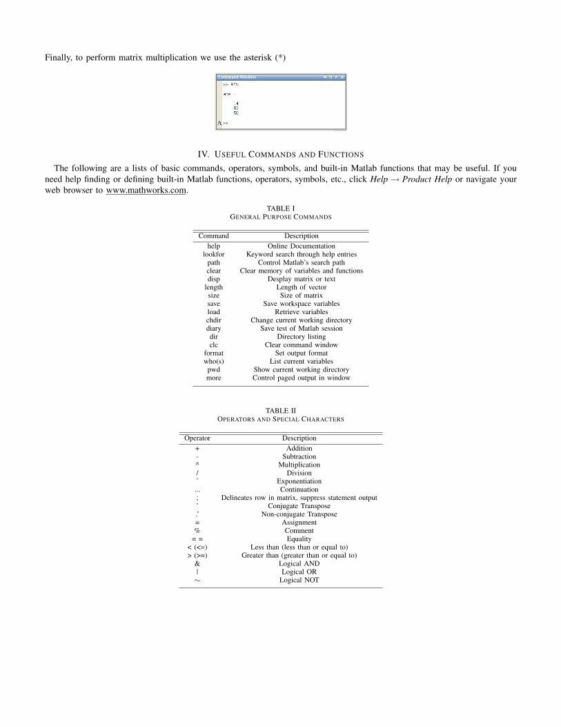
Finally, to perform matrix multiplication we use the asterisk (*)

IV. USEFUL COMMANDS AND FUNCTIONS

The following are a lists of basic commands, operators, symbols, and built-in Matlab functions that may be useful. If youneed help finding or defining built-in Matlab functions, operators, symbols, etc., click Help→ Product Help or navigate yourweb browser to www.mathworks.com.

TABLE IGENERAL PURPOSE COMMANDS

Command Descriptionhelp Online Documentation

lookfor Keyword search through help entriespath Control Matlab’s search pathclear Clear memory of variables and functionsdisp Desplay matrix or text

length Length of vectorsize Size of matrixsave Save workspace variablesload Retrieve variableschdir Change current working directorydiary Save test of Matlab sessiondir Directory listingclc Clear command window

format Set output formatwho(s) List current variables

pwd Show current working directorymore Control paged output in window

TABLE IIOPERATORS AND SPECIAL CHARACTERS

Operator Description+ Addition- Subtraction* Multiplication/ Divisionˆ Exponentiation... Continuation; Delineates row in matrix, suppress statement output’ Conjugate Transpose.’ Non-conjugate Transpose= Assignment% Comment

= = Equality< (<=) Less than (less than or equal to)> (>=) Greater than (greater than or equal to)

& Logical AND| Logical OR∼ Logical NOT

TABLE IIILANGUAGE CONSTRUCTS

Construct Descriptionfor Repeat statements a number of times

while Repeat statements until a condition is metif Conditionally execute statements

else, elseif Used with if statementsend Terminate scope of for, while, and if statements

TABLE IVSPECIAL SYMBOLS

Symbol Descriptioni,j Imaginary unit in the complex number systemInf Infinity

NaN Not a Numberpi 3.14159...

TABLE VPLOTTING AND PRINTING

Command Descriptionfigure Creates figure graphics objectplot Plots a vector

subplot Creates axes in tiled positionshold on Retains current plot so subsequent graphs can be addedxlabel Adds text on the x-axis of the figureylabel Adds text on the y-axis of the figuretitle Add graph title

legend Add legend entries to the plotaxis Manually control x and y axesgrid Add grid on the figure

orient Figure orientationprint Print figure or model, save as image or M-file

V. EXAMPLE 1: CLASSIFICATION

Problem:

The FBI is interested in formulating a battery of questions to aid in identifying criminal minds from a randomly selectedset of individuals in the population. The questions are designed so that for each individual the answers are independent in thesense that the answers to any subset of these questions is not affected by and does not affect the answers to any other subsetof the questions.

A sample of 125 subjects with known criminal (class 1) or no criminal (class 2) backgrounds was chosen to design theclassification scheme. Each subject was asked a battery of 10 independent questions. The subjects answer independently. Dataon the results are summarized in the following table.

TABLE VISUBJECT QUESTIONNAIRE DATA

Class 1 Class 2

Question Yes No Unclear Yes No Unclear1 42 22 5 20 31 52 34 27 8 16 37 33 15 45 9 33 19 44 19 44 6 31 18 75 22 43 4 23 28 56 41 13 15 14 37 57 9 52 8 31 17 88 40 26 3 13 38 59 48 12 9 27 24 5

10 20 37 12 35 16 5

Assuming that this data is representative of the entire population consisting of these groups, we would like to use theclassification scheme derived based upon this data to identify the potential for criminal activity of a randomly selected individualfrom the population.

Three people were then interviewed and the result of each interview is a “profile” of answers to the questions. The followingprofiles were taken

TABLE VIIINDIVIDUAL PROFILES

Question Subject 1 Subject 2 Subject 3

1 Y N Y2 N N Y3 Y U N4 N N Y5 Y Y U6 U Y U7 N U N8 U N N9 Y N Y10 U Y Y

Classify each individual into one of the two groups depending on the likelihood for criminal activity.

Solution:

Let {Ai}10i=1 denote the set of events generated from the 10 answers given by any one subject. For the first subjectfor example, A1 = {“The subject has answered YES to Question 1”}. What we are ultimately interested in is the profileof answers associated with any one individual which we will denote as A. Again, for the first person we have A ={“The subject has answered YES to Question 1 and NO to Question 2 and . . . and UNCLEAR to Question 10”}. Mathemat-ically using set theory we write

A =10⋂

i=1

Ai

We will also let Cj denote the event that any subject belongs to class j for j = 1, 2. An intuitive method for deciding classmembership is to associate the individual with class 1 when the following inequality is met

P (C1|A) > P (C2|A) ,

otherwise associate that person with class 2. Baye’s theorem tells us that

P (Cj |A) =P (A|Cj)P (Cj)

P (A)

resulting in an equivalent testP (A|C1)P (A|C2)

>P (C2)P (C1)

The term on the left is typically referred to as a likelihood ratio and the term on the right is a threshold dependent on thea priori probabilities and independent of any answer one might give. From our assumptions about the independence of thequestions in this survey, it follows that

P (A|Cj) = P

(10⋂

i=1

Ai|Cj

)=

10∏i=1

P (Ai|Cj)

resulting in the final likelihood ratio test ∏10i=1 P (Ai|C1)∏10i=1 P (Ai|C2)

>P (C2)P (C1)

To implement a basic program in Matlab, we would like to build a program that inputs a profile and outputs class membershipand/or a likelihood value. We can do this in Matlab by building an M-file function. Building a function is like building anyother M-file script but a function takes variables as inputs and returns new variables as outputs. To begin a function typefunction [op1, op2, . . . ] = FUNCTIONNAME(ip1, ip2, . . . ) at the beginning of the script and save it as FUNCTIONNAME.m

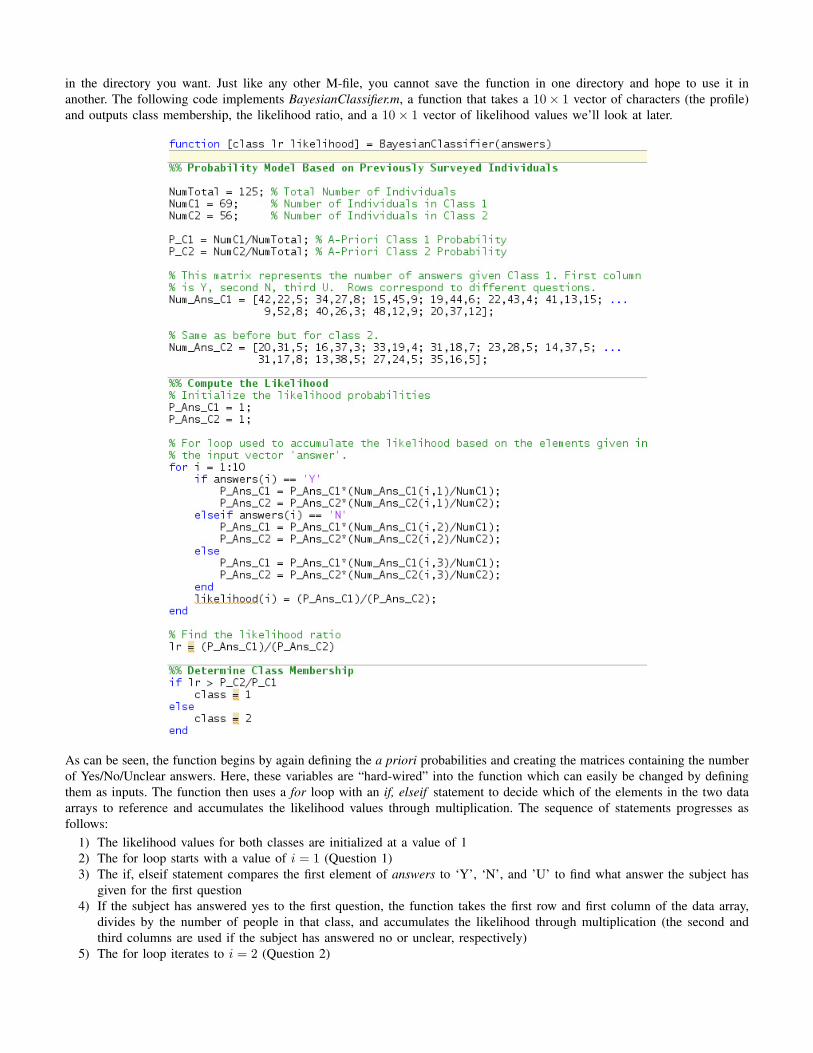
in the directory you want. Just like any other M-file, you cannot save the function in one directory and hope to use it inanother. The following code implements BayesianClassifier.m, a function that takes a 10× 1 vector of characters (the profile)and outputs class membership, the likelihood ratio, and a 10× 1 vector of likelihood values we’ll look at later.

As can be seen, the function begins by again defining the a priori probabilities and creating the matrices containing the numberof Yes/No/Unclear answers. Here, these variables are “hard-wired” into the function which can easily be changed by definingthem as inputs. The function then uses a for loop with an if, elseif statement to decide which of the elements in the two dataarrays to reference and accumulates the likelihood values through multiplication. The sequence of statements progresses asfollows:

1) The likelihood values for both classes are initialized at a value of 12) The for loop starts with a value of i = 1 (Question 1)3) The if, elseif statement compares the first element of answers to ‘Y’, ‘N’, and ’U’ to find what answer the subject has

given for the first question4) If the subject has answered yes to the first question, the function takes the first row and first column of the data array,

divides by the number of people in that class, and accumulates the likelihood through multiplication (the second andthird columns are used if the subject has answered no or unclear, respectively)

5) The for loop iterates to i = 2 (Question 2)

6) The if, elseif statement compares the second element of answers to ‘Y’, ‘N’, and ’U’ to find what answer the subjecthas given for the second question

7) If the subject has answered yes to the second question, the function takes the second row and first column of the dataarray, divides by the number of people in that class, and accumulates the likelihood through multiplication (the secondand third columns are used if the subject has answered no or unclear, respectively)

8) The for loop iterates to i = 3 (Question 3)9) . . .

After all 10 iterations of the for loop, the likelihood ratio is computed and compared to the threshold to decide class membership.In a separate script file, the following code then defines the answer vectors for all three subjects and calls the BayesianClassifierfunction.

The vector likelihood defined earlier in BayesianClassifier.m is a 10× 1 vector showing the accumulated likelihood ratio asone starts with Question 1 and adds questions. Mathematically, the kth element of this vector is described by equation∏k

i=1 P (Ai|C1)∏ki=1 P (Ai|C2)

The following code is then used to graph this vector for all three individuals on the same plot using different colors (the‘LineWidth’ option is used to just make the lines a little wider). Also graphed on the same plot with a dotted line is thethreshold (P (C2)/P (C1) = 56/69). Note that 1:10 creates a row vector of integers from 1 to 10 and ones(1,10) creates a1× 10 row vector with each element equal to one.

VI. EXAMPLE 2: BIVARIATE GAUSSIAN (PEEBLES, SECTIONS 5.3 AND 5.6)

Two random variables X1 ∼ N(µ1, σ21) and X2 ∼ N(µ2, σ

22) are said to be bivariate normal with correlation coefficient ρ

(a number between 0 and 1 with larger values implying greater dependence among the two random variables) if they sharethe joint density function

fX1,X2(x1, x2) =1

2πσ1σ2

√1− ρ2

exp(− 1

2(1− ρ2)

[(x1 − µ1)2

σ21

+(x2 − µ2)2

σ22

− 2ρ(x1 − µ1)(x2 − µ2)σ1σ2

])The following script generates a 3 dimensional view of the joint density using the surface plotting routine

A generalization of the bivariate Gaussian distribution to more than two random variables is the multivariate Gaussiandistribution which is parametrized by a mean vector, µ, and covariance matrix, R. For the bivariate case these can be writtenas

µ =[µ1

µ2

]R =

[σ2

1 ρσ1σ2

ρσ1σ2 σ22

]The following code generates 1000 realizations of two independent standard Normal random variables and defines the 2 × 1mean vector and 2× 2 covariance matrix

The script then produces the 2 × 2 matrix A known as a Cholesky decomposition of R which simply finds the lowertriangular matrix A such that R = AAT (matrix A is like the square-root of R). Realizations of the standard Normal randomvariables are then transformed to two random variables from the bivariate Gaussian distribution described before through anaffine transformation. The hist command is then used to partition the empirical sample space of these two random variablesinto 40 uniformly spaced bins whose locations are given by the variables xout1 and xout2. The variables n1 and n2 give thenumber of realizations that fall into these bins which are normalized so that we may compare them to a pdf.

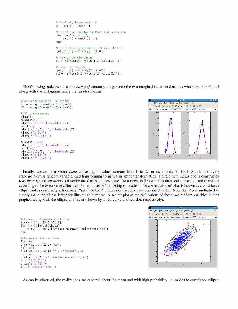
The following code then uses the normpdf command to generate the two marginal Gaussian densities which are then plottedalong with the histograms using the subplot routine.

Finally, we define a vector theta consisting of values ranging from 0 to 2π in increments of 0.001. Similar to takingstandard Normal random variables and transforming them via an affine transformation, a circle with radius one is constructed(cos(theta(i)) and sin(theta(i)) describe the Cartesian coordinates for a circle in R2) which is then scaled, rotated, and translatedaccording to the exact same affine transformation as before. Doing so results in the construction of what is known as a covarianceellipse and is essentially a horizontal “slice” of the 3 dimensional surface plot generated earlier. Note that 2.5 is multiplied tosimply make the ellipse larger for illustrative purposes. A scatter plot of the realizations of these two random variables is thengraphed along with the ellipse and mean (shown by a red curve and red dot, respectively).

As can be observed, the realizations are centered about the mean and with high probability lie inside the covariance ellipse.