ORIGINAL RESEARCH PAPER

Using overlapping sonobuoy data from the Ross Sea to constructa 2D deep crustal velocity model

M. M. Selvans • R. W. Clayton • J. M. Stock •

R. Granot

Received: 13 June 2011 / Accepted: 1 December 2011 / Published online: 20 December 2011

� Springer Science+Business Media B.V. 2011

Abstract Sonobuoys provide an alternative to using long

streamers while conducting multi-channel seismic (MCS)

studies, in order to provide deeper velocity control. We

present analysis and modeling techniques for interpreting

the sonobuoy data and illustrate the method with ten over-

lapping sonobuoys collected in the Ross Sea, offshore from

Antarctica. We demonstrate the importance of using the

MCS data to correct for ocean currents and changes in ship

navigation, which is required before using standard methods

for obtaining a 1D velocity profile from each sonobuoy. We

verify our 1D velocity models using acoustic finite-differ-

ence (FD) modeling and by performing depth migration on

the data, and demonstrate the usefulness of FD modeling for

tying interval velocities to the shallow crust imaged using

MCS data. Finally, we show how overlapping sonobuoys

along an MCS line can be used to construct a 2D velocity

model of the crust. The velocity model reveals a thin crust

(5.5 ± 0.4 km) at the boundary between the Adare and

Northern Basins, and implies that the crustal structure of the

Northern Basin may be more similar to that of the oceanic

crust in the Adare Basin than to the stretched continental

crust further south in the Ross Sea.

Keywords Sonobuoy �Multi-channel seismic � Ross Sea �Finite-difference � 2D velocity model � Crustal structure

Introduction

Using sonobuoys to investigate deep crustal structure

Sonobuoys provide a means of obtaining long offsets for

deep velocity analysis while conducting multi-channel

seismic (MCS) studies. They are preferable to using a long

streamer in locations with difficult open water conditions,

such as in the Ross Sea and Southern Ocean, where

research cruises regularly encounter sea ice, icebergs, and

intense storms. Ocean-bottom seismometers (OBS) provide

another method for collecting active seismic data with

large offsets, but are more expensive than sonobuoys and

are challenging to recover in the conditions described

above. Sonobuoys are also an ideal method for collecting

large offset seismic data in other settings where ship nav-

igation is constrained, such as locations with ship traffic

and narrow bodies of water such as fjords.

Marine refraction seismology has long been recognized

as an essential technique for mapping the sedimentary rock

and basement structure of the Antarctic margins (e.g.,

Ewing and Heezen 1956; see also Anderson 1999 and

references therein). We present techniques for interpreting

deep crustal structure from overlapping sonobuoy data

collected in the northwestern Ross Sea. We first demon-

strate the necessity and method for correcting for the effect

of currents and changes in ship navigation, prior to using

standard processing techniques to obtain 1D velocity

models from the sonobuoys. Second, we explore the ben-

efits of using finite-difference (FD) method modeling of

sonobuoys to tie interval velocities to the shallow crustal

M. M. Selvans � R. W. Clayton � J. M. Stock

Seismological Laboratory, California Institute

of Technology, 1200 E. California Blvd., MC 252-21,

Pasadena, CA 91125, USA

M. M. Selvans (&)

Center for Earth and Planetary Studies, National Air

and Space Museum, Smithsonian Institution, MRC 315,

Washington, DC 20560, USA

e-mail: selvans@gps.caltech.edu

R. Granot

Department of Geological and Environmental Sciences,

Ben-Gurion University of the Negev, Beer Sheva, Israel

123

Mar Geophys Res (2012) 33:17–32

DOI 10.1007/s11001-011-9143-z

structure imaged with MCS data. Finally, we apply these

methods to a set of ten overlapping sonobuoys in order to

construct a 2D velocity model of the deeper crustal struc-

ture along an MCS line.

Modeling methods for seismic refraction data

The FD method is useful for modeling propagation of

seismic waves, including turning waves and their reflec-

tions and conversions at interfaces, for complex subsurface

structure. Ray tracing is similarly useful, but has difficulty

predicting the amplitudes of refracted energy, with the

consequence that it is often difficult to judge the impor-

tance of some of the predicted arrivals. One advantage of

using the FD method to model seismic refraction data is the

ability to model the entire wave front from source to

receiver, which allows us to both tie the shallow structure

detected with MCS data to particular velocity horizons and

to determine the deeper crustal velocity structure.

Shipp and Singh (2002) used a 2D elastic finite-differ-

ence forward model and an iterative full wavefield inver-

sion scheme to best fit their streamer data (with a 12 km

Fig. 1 a Sonobuoy processing methods are developed for data

collected in the northwestern Ross Sea (black box), offshore from

Antarctica. b We interpret a subset of the active seismic data collected

in the northwestern Ross Sea during research cruise NBP0701, shown

on top of multibeam bathymetry (NBP0701 Data Report 2007). Ten

sonobuoys are closely spaced along multi-channel seismic (MCS)

Line 14, which runs from deep water in the Adare Basin onto the

continental margin in the Northern Basin

18 Mar Geophys Res (2012) 33:17–32

123

offset), solving for velocity structure down to 4 km below

the seafloor. This approach is computationally demanding,

with residuals from the comparison of data and the model

being back propagated for every time step, which is why

they were constrained to analysis of relatively shallow

crust. Jones et al. (2007) performed a similar analysis on

streamer data (with offsets of 15 and 18 km); they addi-

tionally derived 1D velocity models from the intercept-

time-slowness (s-p) domain, and downward continued the

data in order to create an image of the layers at depth. They

were able to image the velocity structure to a depth of

6 km.

In order to conduct a marine seismic refraction

experiment with an offset larger than tens of kilometers,

Ritzmann et al. (2004) used OBS instruments. They used

a ray tracing model to reproduce the data, and found that

crustal thickness varied widely, from 32 km for the con-

tinental crust of Svalbard to as little as 2 km (excluding

the *2 km of sediment on top of the basement) near the

margin between continental and oceanic crust. Mantle

velocities are generally [8.0 km/s, but were found to be

as low as 7.7 km/s west of Molloy transform fault, where

the mantle is likely serpentinized (Ritzmann et al. 2004).

Also offshore from Svalbard, Geissler and Jokat (2004)

Fig. 2 Raw data for Sonobuoys

1 (a) and 4 (b) on Line 14 show

key features used to determine

the 1D velocity profile at these

locations. Time is equivalent to

two-way travel time, and

distance is relative to the airgun

source. The direct arrival comes

in first in time for smaller

offsets, while energy from head

waves traveling along layer

interfaces at depth comes in first

for larger offsets; the slopes

of these linear features are

determined by the interval

velocities in the crust. The

hyperbolic reflection from the

seafloor comes in second for

smaller offsets and provides

a time constraint used to

determine the water layer

thickness. Later hyperbolic

features are multiples of the

seafloor reflection. A bandpass

filter of 5, 15, 35, and 40 Hz

is applied to the data

Mar Geophys Res (2012) 33:17–32 19

123

used sonobuoy data as 1D velocity profile ‘‘pseudo-

boreholes’’ along an MCS line to obtain deeper crustal

structure.

Collecting sparse sonobuoy data along MCS lines and

modeling the resulting profiles with ray tracing methods

has been used to investigate deep crustal structure along

Antarctic continental margins as well, for example offshore

from Wilkes Land (Close et al. 2009) and Enderby and

Mac. Robertson Lands (Stagg et al. 2004). In this study, we

combine the analysis of sonobuoy data in the s-p domain

with FD modeling of the waveform to derive a sequence of

overlapping 1D velocity models, which are then interpreted

into a 2D deep crustal velocity model.

Seismic data in the Ross Sea

We will illustrate the analysis procedure for sonobuoy data

collected in the Adare Trough region of the Ross Sea,

offshore from Antarctica (Fig. 1a). The Adare Trough, a

dead mid-ocean spreading ridge, lies in the deep water of

the Adare Basin and trends southward toward the Northern

Basin, which is located up on the continental shelf

(Fig. 1b). How seafloor spreading was linked to extension

in the West Antarctic Rift System to the south is of major

interest, yet still poorly resolved. Shallow structure is well

imaged by MCS data (Granot et al. 2010). However,

understanding the tectonics in the area requires knowledge

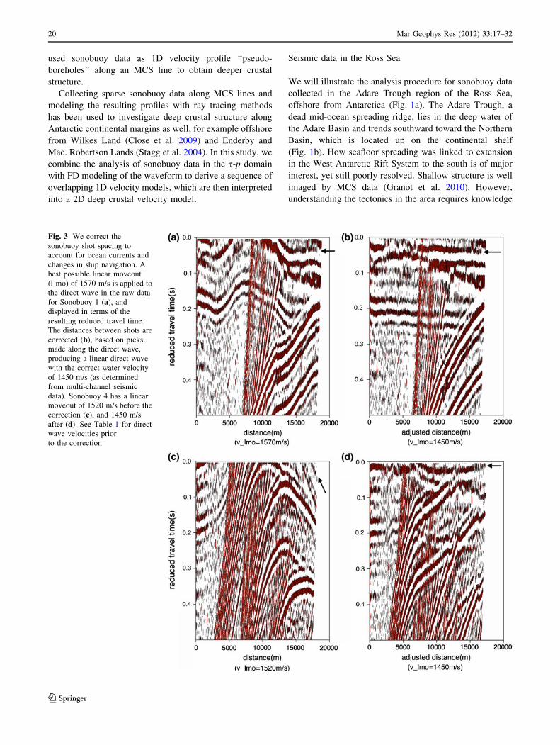
Fig. 3 We correct the

sonobuoy shot spacing to

account for ocean currents and

changes in ship navigation. A

best possible linear moveout

(l mo) of 1570 m/s is applied to

the direct wave in the raw data

for Sonobuoy 1 (a), and

displayed in terms of the

resulting reduced travel time.

The distances between shots are

corrected (b), based on picks

made along the direct wave,

producing a linear direct wave

with the correct water velocity

of 1450 m/s (as determined

from multi-channel seismic

data). Sonobuoy 4 has a linear

moveout of 1520 m/s before the

correction (c), and 1450 m/s

after (d). See Table 1 for direct

wave velocities prior

to the correction

20 Mar Geophys Res (2012) 33:17–32

123

of the deep velocity structure, for example the Moho depth

along the continental shelf break (see Selvans et al. (sub-

mitted) for an analysis of all sonobuoy data, and implica-

tions for tectonics).

We collected seismic reflection and refraction data

during research cruise NBP0701 on board the R/VIB

Nathaniel B. Palmer. Sonobuoy data were collected in the

Adare and Northern Basins, with maximum offsets from

the ship of 20–30 km. Sonobuoys presented here were

deployed with a regular spacing of *15 km (Fig. 1b inset)

in order to obtain overlapping records, since data was

generally returned from as far as 20–30 km from the ship.

Most sonobuoy studies in the western Ross Sea have

focused on basins south of the Northern Basin, and have

used linear moveout and ray tracing methods to determine

sediment velocity gradients and basement depth (Houtz

and Davey 1973; Cooper et al. 1987; Cochrane et al. 1995).

Ocean bottom seismic refraction studies have investigated

the deeper crustal structure in the central and southern Ross

Sea, using ray tracing and amplitude modeling methods

(Trehu et al. 1993; Trey et al. 1999). Crustal thickness,

defined as the depth to velocities of [8000 m/s, is as little

as 16 km beneath sedimentary basins underlain by thinned

crust and magmatic intrusions, and 21 km beneath inter-

vening basement highs (Trey et al. 1999).

MCS data from NBP0701 contain resolvable primaries

from up to 2.3 s travel time (i.e., ‘‘two-way travel time’’)

below the seafloor in the Adare and Northern Basins,

revealing variable sediment thickness (Granot et al. 2010).

Migrated MCS data delineate the structure and deformation

of the sedimentary units in the Adare and Northern Basin,

but cannot tie velocity values to the subsurface layers, and

cannot detect crustal structure below the basement rock.

Methods for sonobuoy analysis and interpretation

Trace spacing adjustment and construction of 1D

velocity profiles

MCS data were collected using a 1.2 km, 48-channel

streamer; this short streamer was required due to regular

interactions with sea ice. Data presented here were

obtained using a 6-element Bolt-gun array with a total

capacity of 34.8 liters, with a typical source spacing of

approximately 40 m. We present data analysis methods,

and results, for ten overlapping sonobuoy profiles along

MCS Line 14, which ran from the deep water of the Adare

Basin south onto the shallow-water shelf of the Northern

Basin (see Fig. 1b).

These sonobuoys were deployed approximately every

15 km, and returned data for 20–30 km of offset. While the

source moved away from the sonobuoy launch position at a

nearly uniform speed and direction, sonobuoy drift after

launch (due to ocean currents) and slight variations in ship

navigation led to varying shot spacing in the refraction data

set. We correct for these effects before analysis, modeling,

and interpretation of the data. The sonobuoy data provide

details of the crustal structure to greater depth than the

MCS data along the same line, and directly detect interval

velocities; MCS data are useful in determining the sound

speed (seismic velocity) of the water layer and the shal-

lowest of the rock layers. Consistent with the generally flat

horizons observed in the MCS data, we assume plane

layers for all velocity horizons.

We show the processing steps needed for accurate

interpretation of the sonobuoy data, starting from the

raw data for the deep-water Sonobuoy 1 (Fig. 2a) and

the shallower-water Sonobuoy 4 (Fig. 2b). We highlight

the low-frequency reflected and refracted energy from the

seafloor and within the crust by applying a tapered band-

pass filter to the data, set to 5, 15, 35, and 40 Hz (i.e., data

with frequencies between 15 and 35 Hz are passed through

with their amplitudes unaltered, and data in the ranges

5–15 and 35–45 Hz are passed through with amplitudes

that decrease to zero at the edges of the filter). Several key

features of the data are obvious in these sonobuoy images:

(1) the direct wave, from source to receiver, is the first

arrival at smaller offsets (e.g., 0–8500 m in Fig. 2a), (2) the

reflection from the seafloor comes in next for smaller off-

sets (e.g., 0–6500 m in Fig. 2a), and due to its strength as

well as noise in the data no reflections from deeper layers

are observed at these offsets (subsequent reflections are

seafloor multiples), (3) head waves, refracted energy from

layer interfaces at depth, come in as first arrivals for larger

Table 1 Direct wave velocities, as determined using a best possible

linear moveout fit to the feature, are listed for Sonobuoys 1–10

(S1–S10) on Line 14

Direct wave velocity

before correction (m/s)

S1 1570

S2 1570

S3 1480

S4 1520

S5 1330

S6 1050

S7 1180

S8 1200

S9 1500

S10 1580

The slope of the direct wave is corrected by adjusting the distance

between traces, such that the sonobuoy data has the correct water

velocity value of 1450 m/s

Mar Geophys Res (2012) 33:17–32 21

123

offsets (e.g., 8,500–19,000 m in Fig. 2a). The offset range

of each arrival type varies with water depth and subsurface

layer thicknesses (see Fig. 2b).

We correct sonobuoy shot spacing so that the direct

wave has a slope of 1450 m/s, as determined by applying a

linear moveout to the direct wave in the MCS data (accu-

rate to ±50 m/s). This value for the seismic velocity of the

water layer is consistent along the MCS line, and is

therefore taken as the default value for all sonobuoys; it is

also consistent with measurements of sound speed in water

taken during the cruise. Data from the one expendable

sound velocimeter (XSV) show water velocities within

1441–1451 m/s (to 600 m depth), while expendable

bathythermographs (XBTs, which measure temperature

with depth and use surface measurements of salinity to

compute sound velocity) show water velocities of

1444–1480 m/s at the northern end of MCS Line 14, and

1446–1448 m/s at the southern end of Line 14. These

sensor measurements of sound speed in water are accurate

to ±0.25 m/s.

In order to correct the shot spacing, we adjust the dis-

tance coordinate of each trace, such that the direct wave is

linear and has the correct slope in the distance versus time

plot. The direct wave of Sonobuoy 1 is shown with a linear

moveout applied before (Fig. 3a, with a direct wave

velocity of 1570 m/s) and after (Fig. 3b, with a direct wave

Fig. 4 Linear moveout (l mo)

is applied to the refracted

energy in the distance-adjusted

version of Sonobuoy 1, to

directly measure interval

velocities and associated times

(s). We detect layers with

velocities of 3900 m/s (a),

4400 m/s (b), 5600 m/s (c), and

8000 m/s (d), with head waves

lying within the arrows; the

8000 m/s layer is also shown as

an inset. The latter value is the

only instance of a velocity that

can be interpreted as the Moho.

Refracted energy from the

seafloor is not observed (an

interval velocity of 2200 m/s for

the uppermost sediment layer is

determined from multi-channel

seismic data)

22 Mar Geophys Res (2012) 33:17–32

123

velocity of 1450 m/s) this correction is made; the adjust-

ment for Sonobuoy 4 makes a similar direct wave velocity

adjustment (Fig. 3c, d). Other sonobuoys have larger dis-

crepancies between the direct wave velocities before and

after the correction (see Table 1). Sonobuoy 3 requires the

smallest correction based on water velocity (average ori-

ginal shot spacing of 38.4 ± 1.6 m, and average corrected

shot spacing of 37.5 ± 2.1 m), while Sonobuoy 6 requires

the largest (similarly, 32.1 ± 2.6 m, and when corrected

43.7 ± 3.5 m). This correction will be more straightfor-

ward for sonobuoys with reliable GPS; in that case, the

sonobuoy location will be at least as well known as that of

the MCS streamer.

We directly detect layer velocities, and their associated

times, by applying linear moveout to head waves in the

corrected sonobuoy data. We detect between three and six

distinct layers at depth for each sonobuoy with this method,

as shown in detail for Sonobuoys 1 and 4 (Figs. 4 and 5,

respectively). This same approach yielded a consistent

velocity of 2000 m/s for the shallowest rock layer in seven

out of the ten sonobuoys; in other cases this seafloor head

wave is not visible. Even when it is visible, it is usually

brief (*10 traces) and so less distinct than most other

refractors we measure. For this reason, we verify this layer

velocity by applying a normal moveout to the hyperbolic

arrival of the seafloor reflection in the raw MCS data, and

Fig. 5 Linear moveout (l mo)

is applied to the refracted

energy in the stretch-corrected

version of Sonobuoy 4, directly

measuring interval velocities

and their associated times. We

detect layers with velocities of

2300 m/s (a), 3300 m/s (b),

4400 m/s (c), and 4800 m/s (d),

with head waves lying within

the arrows. Refracted energy

from the seafloor is not

observed (an interval velocity of

2000 m/s for the uppermost

sediment layer is determined

from multi-channel seismic

data)

Mar Geophys Res (2012) 33:17–32 23

123

use it as the first rock layer velocity for all ten sonobuoys;

one exception is Sonobuoy 1, where analysis of MCS data

provides a first rock layer velocity of 2200 m/s. Layer

velocities for all sonobuoys are listed in Table 2.

The velocities and their associated times are used to

calculate the 1D velocity profile for each sonobuoy (e.g.,

Fowler 1990, p. 119–123). Firstly, the water depth and first

rock layer thickness are calculated using velocities (v) and

reflection times (t) from the MCS data (i.e. h1 = 0.5(t1)(v1)).

Secondly, the thicknesses of deeper layers (i = 2, 3, etc. are

rock layers) are determined using standard seismic refrac-

tion analysis:

hi ¼vi

2 cos ðhi;iþ1Þsi�1 �

Xi�1

j¼1

2hj

vjcos ðhj;iþ1Þ

$ %

where ha,b = arcsin(va/vb) and s is the reduced travel time

associated with the layer velocity, obtained when linear

moveout is applied to the sonobuoy data. Additionally, a

direct image of the s-p curve can be obtained by a radon

transform of the data (McMechan and Ottolini 1980); an

example is shown in Fig. 6.

Layer thicknesses are summed to determine layer

depths, resulting in a 1D velocity profile for the sonobuoy.

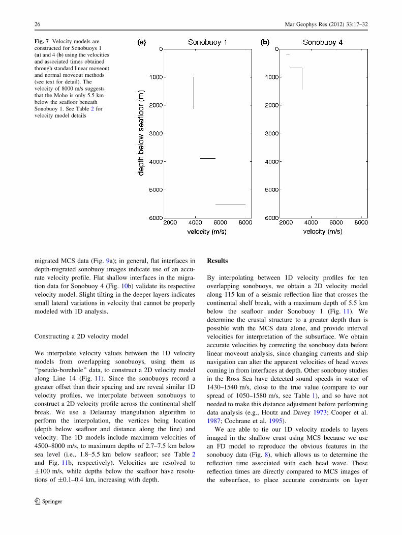
Velocity profiles for Sonobuoys 1 and 4 are plotted with

respect to depth below the seafloor for ease of comparison

(Fig. 7), revealing the unusually high-velocity detail in

Sonobuoy 1, with a maximum velocity of 8000 ± 100 m/s

at 5.5 ± 0.4 km crustal depth. Table 2 lists the details of

the velocity models for all ten sonobuoys.

Finite-difference method modeling and depth migration

We verify our 1D velocity models via finite-difference

(FD) method modeling of the sonobuoys, and by imaging

the subsurface through depth migration of the data. Our FD

model solves the acoustic wave equation in an elastic

medium (Vireaux 1986), using the velocity models calcu-

lated above to reproduce the sonobuoy data (Fig. 8). The

model solutions are 2nd order in time and 8th order in

space; the resulting lack of dispersion of the wave front

through the medium allows for accurate timing. The high

spatial accuracy is required because of the wide range of

velocities in the model (1500–8000 m/s). We assume layer

densities of 2600 kg/m3 for velocities from 2000 to

4000 m/s; 2700 kg/m3 for velocities from 4000 to 6000 m/s;

and 2800 kg/m3 for velocities of 6000 m/s and greater;

Table 2 Velocity model values for Sonobuoys 1–10 (S1–S10) on Line 14 (also see Fig. 10b), and sonobuoy distance along the line

1 (H2O) 2 3 4 5 6 7 8 Distance along the line (km)

S1: d

v

0

1450

1960

2200

2950

3900

4090

4400

5850

5600

7500

8000

0

S2: d

v

0

1450

1780

2000

2320

2200

2520

2800

2910

3700

3660

4400

5000

5000

13

S3: d

v

0

1450

1510

2000

2130

2900

2620

3500

3060

4200

3680

4800

5130

5600

27

S4: d

v

0

1450

1160

2000

1460

2300

1800

3300

2600

4400

2990

4800

38

S5: d

v

0

1450

520

2000

1200

2800

1680

3300

2440

4100

2930

4400

3690

4700

52

S6: d

v

0

1450

500

2000

1010

2500

1270

2800

1800

3500

2500

4100

3040

4500

66

S7: d

v

0

1450

470

2000

1320

3000

2320

4300

2820

4500

78

S8: d

v

0

1450

440

2000

1030

2500

1390

3000

2420

4300

3040

4700

3560

4900

88

S9: d

v

0

1450

470

2000

1020

2400

1250

2900

2020

4000

2700

5000

107

S10: d

v

0

1450

460

2000

1030

2500

1230

2900

1790

3500

2260

4300

2660

4500

3350

4900

114

Sonobuoy 1 lies in the deep water of the Adare Basin, while Sonobuoys 5–10 lie in the shallow water of the Northern Basin. Columns contain the

depth (d, in m) and velocity (v, in m/s) for each layer, as derived from the sonobuoy data. Note that the first rock layer velocity for Sonobuoy 1 is

2200 m/s, while the rest have a velocity of 2000 m/s for this layer; this value is obtained by performing a normal moveout on multi-channel

seismic data at the sonobuoy location. Velocities are resolved to ±100 m/s, while depths below the seafloor have resolutions of ±0.1–0.4 km,

increasing with depth

24 Mar Geophys Res (2012) 33:17–32

123

these densities are consistent with sedimentary, upper crust

(e.g., basement rock), and lower crustal rock respectively

(Jones 1999, p. 64).

By reproducing the sonobuoy data without noise, we

obtain reflection times associated with each head wave.

These allow us to tie the shallow structure observed in the

stacked and migrated MCS data to particular velocity

horizons (Fig. 9). We are therefore able to interpret the

shallow structure revealed by MCS data in terms of directly

observed interval velocities. We additionally extend the

depth to which the crustal velocity structure is delineated,

below the acoustic basement that limits MCS penetration.

We also verify our 1D velocity models by depth

migrating the sonobuoy data (Fig. 10). First a radon

transform is applied to the distance-adjusted sonobuoy

data (e.g., Jones 1999, p. 74–75), which maps the data

into slowness (1/v)—intercept time (s) space (Fig. 6). The

transformed data is then migrated in depth, using the

finite-difference version of the wave-equation method

(Clayton and McMechan 1981), based on the 1D velocity

model.

The subsurface image is in terms of velocity versus

depth, and for Sonobuoy 1 (Fig. 10a) shows flat shallow

layers below the water layer, as observed in the stacked and

Fig. 6 Applying a radon

transform to the model (a) and

data (b) for Sonobuoy 1 reveals

the ellipses that image each

velocity layer in s-p space. The

cusp at the beginning of each

ellipse is defined in terms of the

slowness (p) of the layer (or 1/v,

where v is the velocity), where

layers 1–6 are labeled (1450,

2200, 3900, 4400, 5600, and

8000 m/s respectively). Note

that cusps of layers 1, 4, and 5

are relatively low amplitude,

and that layer 6 is hidden by the

multiple of layer 1

Mar Geophys Res (2012) 33:17–32 25

123

migrated MCS data (Fig. 9a); in general, flat interfaces in

depth-migrated sonobuoy images indicate use of an accu-

rate velocity profile. Flat shallow interfaces in the migra-

tion data for Sonobuoy 4 (Fig. 10b) validate its respective

velocity model. Slight tilting in the deeper layers indicates

small lateral variations in velocity that cannot be properly

modeled with 1D analysis.

Constructing a 2D velocity model

We interpolate velocity values between the 1D velocity

models from overlapping sonobuoys, using them as

‘‘pseudo-borehole’’ data, to construct a 2D velocity model

along Line 14 (Fig. 11). Since the sonobuoys record a

greater offset than their spacing and are reveal similar 1D

velocity profiles, we interpolate between sonobuoys to

construct a 2D velocity profile across the continental shelf

break. We use a Delaunay triangulation algorithm to

perform the interpolation, the vertices being location

(depth below seafloor and distance along the line) and

velocity. The 1D models include maximum velocities of

4500–8000 m/s, to maximum depths of 2.7–7.5 km below

sea level (i.e., 1.8–5.5 km below seafloor; see Table 2

and Fig. 11b, respectively). Velocities are resolved to

±100 m/s, while depths below the seafloor have resolu-

tions of ±0.1–0.4 km, increasing with depth.

Results

By interpolating between 1D velocity profiles for ten

overlapping sonobuoys, we obtain a 2D velocity model

along 115 km of a seismic reflection line that crosses the

continental shelf break, with a maximum depth of 5.5 km

below the seafloor under Sonobuoy 1 (Fig. 11). We

determine the crustal structure to a greater depth than is

possible with the MCS data alone, and provide interval

velocities for interpretation of the subsurface. We obtain

accurate velocities by correcting the sonobuoy data before

linear moveout analysis, since changing currents and ship

navigation can alter the apparent velocities of head waves

coming in from interfaces at depth. Other sonobuoy studies

in the Ross Sea have detected sound speeds in water of

1430–1540 m/s, close to the true value (compare to our

spread of 1050–1580 m/s, see Table 1), and so have not

needed to make this distance adjustment before performing

data analysis (e.g., Houtz and Davey 1973; Cooper et al.

1987; Cochrane et al. 1995).

We are able to tie our 1D velocity models to layers

imaged in the shallow crust using MCS because we use

an FD model to reproduce the obvious features in the

sonobuoy data (Fig. 8), which allows us to determine the

reflection time associated with each head wave. These

reflection times are directly compared to MCS images of

the subsurface, to place accurate constraints on layer

Fig. 7 Velocity models are

constructed for Sonobuoys 1

(a) and 4 (b) using the velocities

and associated times obtained

through standard linear moveout

and normal moveout methods

(see text for detail). The

velocity of 8000 m/s suggests

that the Moho is only 5.5 km

below the seafloor beneath

Sonobuoy 1. See Table 2 for

velocity model details

26 Mar Geophys Res (2012) 33:17–32

123

velocities. This provides a method for determining sedi-

ment thickness, whose structure is otherwise interpreted

(from MCS data) entirely in time space (Granot et al.

2010).

Due to the experimental design and processing methods

we employ, we are able to accurately determine crustal

structure in the Adare and Northern Basins to a greater

depth than is possible with the MCS data. Overlapping

sonobuoys allow us to construct a 2D velocity profile of the

crust more cheaply than is possible with ocean-bottom

seismometers. Since the NBP0701 cruise deployed simi-

larly spaced sonobuoys along other MCS lines in the

southern Adare Basin and northern part of the Northern

Basin, these methods can be used to construct a pseudo-3D

interpretation of the crustal structure in locations where

MCS lines cross (see Selvans et al. (submitted)).

Discussion and conclusions

Obtaining sonobuoy FD models that accurately reproduce

the main features being analyzed allows for further inter-

pretation of MCS data than is otherwise possible. MCS

data image shallow structure in great detail, but cannot

directly measure layer velocities at depth. Matching the

reflection times from each layer of known velocity in the

FD model to the MCS image provides the velocity model

details needed for depth migration of MCS data.

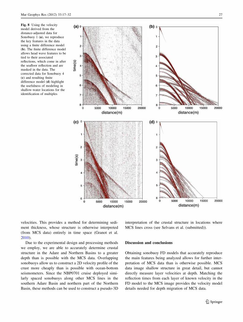
Fig. 8 Using the velocity

model derived from the

distance-adjusted data for

Sonobuoy 1 (a), we reproduce

the key features in the data

using a finite difference model

(b). The finite difference model

allows head wave features to be

tied to their associated

reflections, which come in after

the seafloor reflection and are

masked in the data. The

corrected data for Sonobuoy 4

(c) and resulting finite

difference model (d) highlight

the usefulness of modeling in

shallow-water locations for the

identification of multiples

Mar Geophys Res (2012) 33:17–32 27

123

Modeling sonobuoys using FD has further potential for

sonobuoy data analysis, since refinements in the model can

reveal more details about the crustal structure. For instance,

models could be altered to include head waves that occa-

sionally come in late as a result of interbed multiples,

further refining the 1D velocity model at that sonobuoy

location. An elastic version of the model could be used to

identify the converted phases in the data; an elastic FD

model was run for Sonobuoys 1 and 4 to confirm that none

of the head waves used in this analysis are converted

phases.

Using an elastic FD model would also constrain the

allowable range of shear wave velocities, based on the

amplitude of those phases. Elastic FD models with both

vs = (1/H3)vp and a vs = (1/2H3)vp have converted phases

with amplitudes similar to those of the main head wave

features of the sonobuoy; these phases are not observed in

the data, indicating that shear wave velocities are small.

Modeling the full range of possible shear wave velocities

would help in identifying the crustal lithology, below the

layers that can be mapped in MCS data over long distances

and then tied to borehole results (e.g., Granot et al. 2010).

Modeling of overlapping, and particularly reversed

sonobuoys could additionally include lateral variations in

layer velocity and layer thickness and a smoothly varying

profile with depth, in order to determine whether these

secondary effects are observed in the sonobuoy data.

We show the necessity of adjusting distance between

traces for sonobuoy studies, since ocean currents and

changing speed and direction of the ship can alter the direct

wave slope such that it does not accurately reflect the sound

speed in water of 1450 m/s (see Table 1). Prior to the

correction, direct wave velocities were as much as 130 m/s

higher (Sonobuoy 10) and 400 m/s lower (Sonobuoy 6)

than the true sound speed in water. Directly measuring

layer velocities at depth by applying a linear moveout to

head waves in the uncorrected sonobuoy data will be off

from the true velocities of those layers by similar amounts,

resulting in errors larger than the measurement uncertainty

of ±100 m/s in most cases (seven out of ten sonobuoys).

In order to use the reflected energy features in the

sonobuoy analysis, this error cannot be corrected through a

simple stretch in the time dimension, based on the best fit

direct wave velocity, since a hyperbolic feature will not

retain its proper shape if a linear stretch is applied. Gen-

erally, in cases where direct wave velocities differed from

the true sound speed in water by more than the uncertainty

of the velocity measurement, sonobuoy studies have

reported inaccurate layer velocities.

Finally, our analysis is greatly aided by the experiment

design. Collecting overlapping sonobuoy data along sev-

eral MCS lines during research cruise NBP0701 allows us

to construct 2D velocity models deep within the crust, to a

greatest depth of 5.5 km below the seafloor. This depth is

Fig. 9 Multi-channel seismic (MCS) data from the same location as

Sonobuoy 1 (a) can be compared to the finite difference model (b) in

order to determine the layer velocities within the reflection data. In

the model, reflections from which head waves originate are labeled

with large arrows, while multiples are labeled with small arrows. Note

that the first layer at depth (3900 m/s) corresponds to sediment layers

imaged in the MCS data, the 4400 m/s seems to be the top of the

basement rock, 5600 m/s is within the basement rock, and the

8000 m/s layer is deep in the basement rock (below the seafloor

multiple). Sonobuoy data also determine layer velocities below the

acoustic basement, which is the limit to which reflection data can

delineate subsurface structure

28 Mar Geophys Res (2012) 33:17–32

123

equivalent to 5.0 s travel time below the seafloor, deeper

than the maximum depth of 2.3 s below the seafloor at

which basement rock is imaged with MCS data (Granot

et al. 2010). We regularly determine layer velocities of

4500–5000 m/s, at 2.0–3.0 km below the seafloor, and are

able to see that the velocity contours fit to these data are at

consistent depths along the 115 km of MCS Line 14. Being

able to use the depth penetration and ability to directly

measure layer velocities that sonobuoys provide in order to

construct a 2D velocity model is a particularly useful

analytical technique for locations such as the Ross Sea,

where sea ice conditions preclude the use of a longer MCS

streamer.

Having a deep 2D velocity profile along Line 14 of the

NBP0701 MCS data allows us to begin examining the

crustal structure along the margin between the Adare and

Northern Basins (Fig. 11a). Two distinct features stand out.

One is the unusually thin crust under Sonobuoy 1: the data

Fig. 10 Depth migration is applied to the distance-adjusted data for

Sonobuoy 1 (a) and Sonobuoy 4 (b), using their respective 1D

velocity models. Parallel bedding, as observed in the multi-channel

seismic data (e.g., Fig. 8a), indicates a good model fit to the data;

slight tilting in deeper layers indicates small lateral variations in

velocity that cannot be properly modeled with 1D analysis

Mar Geophys Res (2012) 33:17–32 29

123

reveal a maximum velocity of 8000 m/s at 5.5 km below

the seafloor, which is interpreted as the Moho. Since there

is 2.1 km of overlying sediment at this location (as indi-

cated by comparing reflection time of the 4400 m/s layer in

the FD model with that of acoustic basement as imaged

with MCS data (see Fig. 9), and referring to the 1D

velocity model of Sonobuoy 1 for the depth of that layer),

the igneous crustal thickness is 3.4 km.

Although unusual, similarly thin crustal thicknesses are

observed in the Ross Sea (4–27 km; see Anderson (1999)

and references therein), and in continental margins of East

Antarctica (\4 km in continental crust offshore from

Fig. 11 The 2D velocity

structure along Line 14 is

determined to a depth of 5.5 km

below the seafloor. Seafloor

bathymetry (a) provides context

for the 2D velocity model

(b) interpolated from velocity

models for ten overlapping

sonobuoys (c). Layer interfaces

observed in the data are

indicated with an ‘‘x’’ (see

Table 2 for details); vertical

exaggeration is 1:8. Sediment

layers (*2000–4000 m/s)

thicken slightly from the Adare

Basin (Sonobuoy 1) to the

Northern Basin (Sonobuoys

5–10), as expected for moving

up a shelf break onto a

sediment-filled basin.

Interestingly, deeper velocity

contours remain approximately

flat along the line, whereas if the

shelf break were the transition

from oceanic to continental

crust, we would expect these

contours to deflect down under

the Northern Basin.

Uncertainties on 2D velocity

contours are ±200 m/s and

±100–500 m (increasing

with depth)

30 Mar Geophys Res (2012) 33:17–32

123

Wilkes Land (Close et al. 2009), and 4 km in oceanic crust

offshore from Enderby Land (Stagg et al. 2004)). Results

from processing all NBP0701 sonobuoys, including the

interpolation of additional 2D velocity models, are dis-

cussed in the context of other tectonic settings similar to

that of the Adare and Northern Basin region by Selvans

et al. (submitted).

The other obvious feature is that all well-constrained

velocity contours (2000–5400 m/s) are approximately flat,

considering the 8:1 vertical exaggeration (Fig. 11), indi-

cating that it is unlikely for there to be significant local

relief on layer interfaces within the crust. Velocity contours

at a transition between oceanic and continental crust would

be expected to deflect downward under the thicker conti-

nental crust, suggesting that the continental shelf break

between the Adare and Northern Basins (obvious in

bathymetry) may not be the location of the transition

between crustal types. As also suggested by Cande and

Stock (2006), who discussed the possibility of the Northern

Basin crust being ‘transitional,’ based on analysis of

magnetic anomaly data, we find that the crustal structure

may be continuous across the shelf break.

Acknowledgments We would like to thank Captain Mike Watson,

the crew, and the Raytheon Polar Services Corporation technical staff

on board the Nathaniel B. Palmer. This study was supported by

National Science Foundation grants OPP04-40959 (S. Cande) and

OPP-0440923 and OPP-0944711 (J. Stock and R. Clayton).

References

Anderson JB (1999) Antarctic marine geology. Camb University

Press, Cambridge

Cande SC, Stock JM (2006) Constraints on the timing of extension in

the Northern Basin, Ross Sea. 9th International symposium on

Antarctic earth science proceeding

Clayton R, McMechan G (1981) Inversion of refraction data by wave

field continuation. Geophysics 46:860–868

Close DI, Watts A, Stagg H (2009) A marine geophysical study of the

Wilkes Land rifted continental margin, Antarctica. Geophysical

J Int 177(2):430–450

Cochrane GR, De Santis L, Cooper AK (1995) Seismic velocity

expression of glacial sedimentary rocks beneath the Ross Sea

from sonobuoy seismic-refraction data, geology and seismic

stratigraphy of the Antarctic margin. Antarctic Res Ser 68:

261–270

Cooper A, Davey F, Cochrane G (1987) Structure of extensionally

rifted crust beneath the western Ross Sea and Iselin Bank,

Antarctica, from sonobuoy seismic data. The Antarctic conti-

nental margin: geology and geophysics of the Western Ross Sea.

Published by the Circum-Pacific Council of Energy and Mineral

Resources, Earth Science Ser 5B:93–117

Ewing M, Heezen BC (1956) Some problems of Antarctic submarine

geology. In: Carey AP, Gould LM, Hulbert EO, Odishaw H,

Smith WE (eds) Antarctica in the IGY. Geophys Monogr 1,

pp 75–81

Fowler CMR (1990) The solid earth: an introduction to global

geophysics. Camb University Press, CambridgeFig. 11 continued

Mar Geophys Res (2012) 33:17–32 31

123

Geissler WH, Jokat W (2004) A geophysical study of the northern

Svalbard continental margin. Geophysical J Int 158(1):50–66

Granot R, Cande S, Stock J, Davey F, Clayton R (2010) Postspreading

rifting in the Adare Basin, Antarctica: regional tectonic conse-

quences. Geochem Geophys Geosyst 11(8):Q08005. doi:10.1029/

2010GC003105

Houtz R, Davey F (1973) Seismic profiler and sonobuoy measure-

ments in Ross Sea, Antarctica. J Geophys Res 78(17):3448–3468

Jones EJW (1999) Marine geophysics. Wiley, London

Jones GD, Barton PJ, Singh SC (2007) Velocity images from stacking

depth-slowness seismic wavefields. Geophys J Int 168(2):583–

592

McMechan GA, Ottolini R (1980) Direct observation of a p-s curve in

a slant stacked wave field. Bull Seismol Soc Am 70(3):775

NBP0701 Data Report (2007) prepared by Ayers J. Available at http://

www.marine-geo.org/tools/search/data/field/NBPalmer/NBP0701/

docs/NBP0701Report.htm

Ritzmann O, Jokat W, Czuba W, Guterch A, Mjelde R, Nishimura Y

(2004) A deep seismic transect from Hovgard Ridge to north-

western Svalbard across the continental ocean transition: a

sheared margin study. Geophys J Int 157(2):683–702

Selvans MM, Stock JM, Clayton RW, Cande S, Davey F, Granot R

(submitted Sept. 30, 2011) Deep crustal structure of the Adare

and Northern Basins, Ross Sea, Antarctica, from sonobuoy data.

J Geophys Res

Shipp RM, Singh SC (2002) Two dimensional full wavefield inversion

of wide aperture marine seismic streamer data. Geophys J Int

151(2):325–344

Stagg HMJ, Colwel J, Direen N, OıBrien P, Bernardel G, Borissova I,

Brown B, Ishirara T (2004) Geology of the continental margin of

Enderby and Mac. Robertson Lands, East Antarctica: insights

from a regional data set. Marine Geophys Res 25(3):183–219

Trehu A, Behrendt JC, Fritsch J (1993) Generalized crustal structure

of the Central basin, Ross Sea, Antarctica. In: Damaske D,

Fritsch J (eds) German Antarctic North Victoria Land Expedition

1988/1989. Bundesanstalt fur Geowissenschaften und Rohstoffe,

Hannover, pp 291–311

Trey H, Cooper AK, Pellis G, della Vedova B, Cochrane G,

Brancolini G, Makris J (1999) Transect across the West

Antarctic rift system in the Ross Sea, Antarctica. Tectonophysics

301(1–2):61–74

Vireaux J (1986) P-SV wave propagation in heterogeneous media:

velocity-stress finite difference method. Geophysics 51:889–901

32 Mar Geophys Res (2012) 33:17–32

123