1

Using Persistent Homology to Quantify a DiurnalCycle in Hurricane Felix

Sarah Tymochko, Elizabeth Munch, Jason Dunion, Kristen Corbosiero, and Ryan Torn

Abstract—The diurnal cycle of tropical cyclones (TCs) is adaily cycle in clouds that appears in satellite images and mayhave implications for TC structure and intensity. The diurnalpattern can be seen in infrared (IR) satellite imagery as cyclicalpulses in the cloud field that propagate radially outward fromthe center of nearly all Atlantic-basin TCs. These diurnal pulses,a distinguishing characteristic of the TC diurnal cycle, beginforming in the storm’s inner core near sunset each day andappear as a region of cooling cloud-top temperatures. The areaof cooling takes on a ring-like appearance as cloud-top warmingoccurs on its inside edge and the cooling moves away from thestorm overnight, reaching several hundred kilometers from thecirculation center by the following afternoon. The state-of-the-artTC diurnal cycle measurement has a limited ability to analyze thebehavior beyond qualitative observations. We present a methodfor quantifying the TC diurnal cycle using one-dimensionalpersistent homology, a tool from Topological Data Analysis, bytracking maximum persistence and quantifying the cycle usingthe discrete Fourier transform. Using Geostationary OperationalEnvironmental Satellite IR imagery data from Hurricane Felix(2007), our method is able to detect an approximate daily cycle.

Index Terms—Topological Data Analysis, Atmospheric Science,Hurricane, Diurnal Cycle

I. INTRODUCTION

THE field of atmospheric science has numerous observa-tion platforms that provide high space and time resolution

data, but has yet to find methods which can quantify theintuitive patterns explicitly. Meanwhile, the young field ofTopological Data Analysis (TDA) encompasses methods forquantifying exactly these sorts of structural intuitions seenby atmospheric scientists. This paper merges these two fieldsby using persistent homology, a now well-established tool inTDA, to quantify a diurnal cycle observed in a hurricane usingGeostationary Operational Environmental Satellite (GOES)infrared (IR) satellite data.

Persistent homology, and more generally TDA methods,has found significant success in rather disparate applicationsby finding structure in data and using this insight to answerquestions from the domain of interest. For instance, Giustiet al. used the homology of random simplicial complexesto investigate the geometric organization of neurons in ratbrains [1]. Nicolau et al. used mapper, another tool in TDA,to discover a new subtype of breast cancer [2]. More closely

ST and EM are with the Dept. of Computational Mathematics, Scienceand Engineering at Michigan State University. EM is also with the Dept. ofMathematics at MSU. KC and RT are with the Dept. of Atmospheric and En-vironmental Sciences at University at Albany - SUNY Albany. JD is affiliatedwith Cooperative Institute for Marine and Atmospheric Studies, University ofMiami, and Hurricane Research Division, NOAA/Atlantic Oceanographic andMeteorological Laboratory, Miami, Florida.

Corresponding author: ST, e-mail: tymochko@egr.msu.edu.

related to this work is the use of TDA for time series analysisand image processing. This includes using persistent homologyto understand periodicity in time series arising from biological[3], [4] and engineering applications [5]. There has also beena great deal of interest in using persistence for image analysis,e.g. [6], [7], [8], [9].

This paper presents an application of the use of both timeseries and image analysis using TDA. The diurnal cycle oftropical cyclones (TCs) has been described in previous studies[10], [11], [12], [13], [14], [15], [16], [17], [18] that provideevidence of the regularity of this cycle as well as its potentialimpacts. This diurnal pattern can be seen in GOES IR imageryas cyclical pulses in the cloud field that propagate radiallyoutward from TCs at speeds of 5-10 m s−1 [10], [11], [15].These diurnal pulses, a distinguishing characteristic of the TCdiurnal cycle, begin forming in the TC’s core near the timeof sunset each day and appear as a region of cooling cloud-top temperatures. The area of cooling then takes on a ring-like appearance as marked cloud-top warming occurs on itsinside edge and it moves away from the storm overnight,reaching several hundred kilometers from the TC center bythe following afternoon. Observations and numerical modelsimulations indicate that TC diurnal pulses propagate througha deep layer of the TC environment, suggesting that they mayhave implications for TC structure and intensity [10], [11],[15], [17].

The current state of the art TC diurnal cycle measurementhas a limited ability to analyze the behavior beyond qualitativeobservations. This paper presents a more advanced mathemat-ical method for quantifying the TC diurnal cycle using toolsfrom TDA, namely one-dimensional persistent homology toanalyze the holes in a space. This research aims to detect thepresence of the diurnal cycle in GOES IR satellite imageryand to track the changes through a time series.

The first attempt, using the naive combination of persistenthomology with the GOES IR imagery, did not show therecurring pattern. Due to the drastically variable values inthe IR brightness temperature data, persistent homology wasnot able to detect any significant structure. Looking at thedata, however, there is a clear circular feature visible, so wedeveloped more sophisticated methods to extract this structure.

In this paper, we present a method applying the distancetransform and one-dimensional persistent homology, allowingus to quantify the cycle using maximum persistence. We showthat using tools from TDA, we can detect cyclic behavior inthe hurricane that repeats approximately every 24 hours.

arX

iv:1

902.

0620

2v1

[cs

.CV

] 1

7 Fe

b 20

19

2

II. TROPICAL CYCLONE BACKGROUND

Previous research has documented a clear diurnal cycle ofcloudiness and rainfall in TCs: enhanced convection (i.e., thun-derstorms) occurs overnight, precipitation peaks near sunrise,and upper-level cloudiness (i.e., the cirrus canopy) expandsradially outward throughout the day, reaching its maximumareal coverage in the early evening hours [10], [11], [12],[13], [14], [15], [16], [17], [18]. To quantity the expansionand contraction of the cirrus canopy, Dunion et al. usedGOES satellite IR imagery to examine the six-hour cloud-toptemperature differences of major hurricanes in the Atlanticbasin from 2001 to 2010 [10]. They found that an area ofcolder cloud tops propagated outward around 5-10 m s−1 overthe course of the day, with warming temperatures on its inneredge. More recently, in [15], Ditchek et al. expanded Dunionet al.’s work to include all tropical cyclones in the Atlanticbasin from 1982 to 2017 and found that the diurnal pulse isnearly ubiquitous, with 88% of TC days featuring an outwardlypropagating pulse.

Despite the consistent signature and documentation of thisdiurnal cloud signature, open questions remain as to howthe diurnal cycle is linked to inner-core convective processesand whether it is a column-deep phenomenon or mainly tiedto upper-level TC cloud dynamics related to incoming solarradiation [12], [13], [14], [15]. Investigating these questionsis relevant to TC forecasting as the diurnal cycle of cloudsand rainfall has implications for forecasting storm structureand intensity, as evidenced by the diurnal cycle in objec-tive measures of TC intensity and the extent of the 50-ktwind radius documented by Dunion et al. Additionally, andespecially relevant to the current work, most of the papersabove have identified the pulse using subjective measuresof cloud-top temperature change and timing [10], [15]. Thecurrent work seeks to quantify the pulse to determine its trueperiodicity using persistent homology, a topological tool thatis particularly effective at capturing the type of patterns visiblein the pulse.

III. MATH BACKGROUND

Persistent homology is a tool from the field of TDA whichmeasures structure in data. This data can start in many forms,including as point clouds or, as in the case of this work, as afunction on a domain. In this section, we will briefly reviewthe necessary background to understand cubical homologyand persistent homology, and refer the interested reader to[19], [20], [21], [22], [23] for a more complete introduction.Additionally, we will introduce tools used in our method,including the distance transform, mathematical morphology,and the Fourier transform.

A. Cubical complexes

In this section, we largely follow Chapter 2 of [19] with thecaveat for the informed reader that because we use homologywith Z2 coefficients, we can be lazy about orientations ofcubes. In addition, our data consists of 2D images, so weneed only define cubes up to dimension 2.

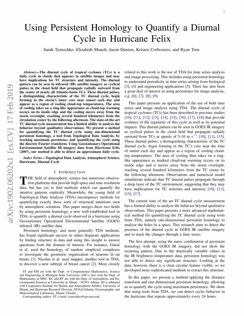
Fig. 1. An example of K for representing a 7 × 7 matrix is shown atleft. A subset of this complex is shown at right. The red dashed loop andthe green bold loop represent equivalent classes in H1(Mr). The bold blueloop represents a different equivalence class in H1(Mr). For this example,H1(Mr) has rank 3.

An elementary interval is a closed interval I ⊂ R of theform [`, `+1] or [`] for ` ∈ Z, which are called nondegenerateand degenerate respectively. An elementary cube Q ∈ R2 is aproduct of elementary intervals Q = I1 × I2. The dimensionof Q, dim(Q), is the number of nondegenerate componentsof Q. Note that 0-dimensional cubes are just vertices at thepoints on the lattice Z × Z in R2, 1-dimensional cubes areedges connecting these vertices, and 2-dimensional cubes aresquares. Let K denote the set of all elementary cubes in R2

and Kd ⊂ K the set of d-dimensional cubes. A set X ⊂ R2 iscubical if it can be written as a finite union of elementarycubes. Then we denote the associated cubical complex asK(X) = {Q ∈ K | Q ⊂ X}, with the d-dimensional subsetdenoted Kd(X) = {Q ∈ K(X) | dim(Q) = d}. If Q ⊆ P ,then we say Q is a face of P , denoted Q ≤ P . If Q ( P , thenQ is a proper face of P , denoted Q < P , and is additionallya primary face of P if dim(Q) = dim(P )− 1.

A greyscale image, or more generally an m×n matrix, canbe viewed as a function M : D → R where

D = {(i, j) | 0 ≤ i < m, 0 ≤ j < n}.

We will model this as a function defined on a particularlysimple cubical set K = K([0,m] × [0, n]); see the left ofFig. 1 for an example. For simplicity, we denote by si,j thesquare [i, i+ 1]× [j, j + 1].

So, given a matrix M , we equivalently think of this data asa function M : K → R where we set M(si,j) equal to thematrix entry Mi,j and set M(P ) = minsi,j>P M(si,j) for alllower dimensional cubes P . Note that we will abuse notationand use M to denote both the original matrix and the view ofthis matrix as a function with domain K.

B. Distance transform

The distance transform is a tool used in image processingand is computed on binary images [24], [25]. It is used in vari-ous applications in many disciplines, such as guiding robots tonavigate obstacles [26], computing geometric representationssuch as Voronoi diagrams [27] as well as being a usefulmethod in many other image processing tools [28].

This operation assigns each pixel in the foreground (pixelswith value 1) a value based on its distance to a pixel in thebackground (pixels with value 0). This can be computed using

3

various distance metrics, most frequently the L1, L2 or L∞distance.

Using the notation from the previous section, si,j representsthe pixel, (i, j) in the image represented as a matrix of pixels,M . Given any si,j ∈M

min d(si,j , x)

where x is a 0-valued pixel and d is any distance metric.Given two pixels, si1,j1 , si2,j2 we calculate the L∞ distance,also called the chessboard distance, between them as

d(si1,j1 , si2,j2) = max{|i2 − i1|, |j2 − j1|}.

This defines a distance on the pixels, which are the 2-cellsin the cubical complex. The distance can be extended to thelower dimensional cells in the same manor as described inSec. III-A.

C. Homology

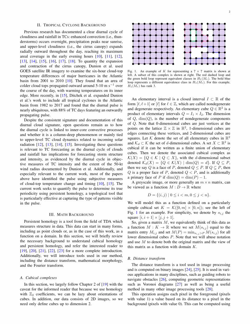
Homology [20], [29] is a standard tool in algebraic topologywhich provides a vector space1 Hk(X) for each dimensionk = 0, 1, 2, . . . for a given topological space X . The differ-ent dimensions measure different properties of the space. Inparticular, for this work we are interested in 1-dimensionalhomology; i.e. when k = 1. The 1-dimensional homologygroup measures the number of loops in the space; equivalently,we can think of this as the number of holes in the space.In particular, if we look at the black region in each of theexamples in Fig. 2, the rank of the first homology for each is(1,1,1,2,2,3).

The exact definition of homology is as follows. For anycubical set L (which for the purposes of this discussion willalways be a subset of K), we have sets giving the cubes ofdifferent dimensions: Ki(L) for i = 0, 1, 2. An i-chain is aformal linear combination of i-simplices in L,

c =∑

Qj∈Ki(L)

ajQj ,

with coefficients aj ∈ Z2. We can of course add these objectsby setting (

∑ajQj) + (

∑bjQj) =

∑(aj + bj)Qj and

multiply by a constant. Thus, the collection of all i-chainsforms a vector space Ci(L).

We define a linear transformation

δi : Ci(L)→ Ci−1(L)

called the boundary map, by setting δi(Q) =∑P where the

sum2 is over the primary faces P < Q. The kernel of δ1,Ker(δi), (that is, the set of elements of C1(L) which map to0) is generated by closed loops in L. The image of δ2, Im(δ2),is generated by boundaries of 2-cells. Then the 1-dimensionalhomology group is defined to be H1(K) = Ker(δ1)/Im(δ2).An element of this group γ ∈ H1(L), represents an equiva-lence class of loops which can differ by collections of 2-cells;see the right side of Fig. 1 for an example of two loops whichare equivalent in H1(L).

1Normally a group, however, we are working with field coefficients.2Again, notice that because we are working with Z2 coefficients, the book-

keeping normally needed for orientation is unnecessary.

D. Persistent Homology

For a static space L, H1(L) measures information aboutthe number of loops. Persistent homology takes as input achanging topological space, and summarizes the informationabout how the homology changes.

Let an m× n R-valued matrix M be given. Fix a functionvalue r ∈ R and let Mr = f−1(−∞, r]. That is, Mr is thesubset of squares in Km×n which have value at most r in thematrix, along with all edges and vertices which are faces ofany included square. Mr is often called a sublevel set of M .See the right side of Fig. 1 for an example of the structureof K and see Fig. 2 for Mr regions corresponding to thematrix on the left of Fig. 2. This shows Mr drawn in blackfor r = 0.6, 0.9, 1.03, 1.1, 1.2, and 1.23.

These spaces have the property that Mr ⊆ Ms for r ≤ s,thus we can consider the sequence

Mr1 ⊆Mr2 ⊆ · · · ⊆Mrk (1)

for any set of numbers r1 < r2 < · · · rk. This sequence ofspaces is called a filtration. For each of the spaces, we cancompute the homology group Hp(Mri). The inclusion mapsof Eqn. (1) give rise to linear maps

Hp(Mr1)→ Hp(Mr2)→ · · · → Hp(Mrk).

It is these maps that we study to understand how the spacechanges. In particular, when we are focused on 1-dimensionalhomology (k = 1) as in this study, a loop is represented byan element γ ∈ H1(Mri). We say that this loop is born atri if it is not in the image from the previous space; that is,γ 6∈ Im(H1(Mi−1)→ H1(Mi)). This same loop dies at rj if itmerges with this image in Mrj ; that is, γ ∈ Im(H1(Mi−1)→H1(Mj)) where we abuse notation by using γ to both referto the class in H1(Mri) and the image of this class underthe sequence of maps in H1(Mrj ). We refer to rj − ri as thelifetime of the class.

A persistence diagram,as seen in the right of Fig. 2, is acollection of points where for each class which is born atri and dies at rj is represented by a point at (ri, rj). Theintuition is that a class which has a long lifetime is far fromthe diagonal while a class with a short lifetime is close. Inmany cases, a long lifetime loop implies that there is some sortof inherent topological feature being found, and thus that thispoint far from the diagonal is important, while short lifetimeloops are likely caused by topological noise due to samplingor other errors in the system. In the example of Fig. 2,there is a prominent off-diagonal point which shows that thefunction defined by the matrix has a circular feature. Thus,a common measure for looking at the persistence diagramwhen investigating a single, circular structure is the maximumpersistence, defined as

MaxPers(D) = max(ri,rj)∈D

rj − ri

for a given persistence diagram, D.

E. Mathematical morphology

Mathematical morphology is a broad field based on ana-lyzing shapes of objects using mathematical tools from areas

4

Fig. 2. An example matrix, M (top left) and corresponding persistencediagram (top right). Second and third row: The black portions are sublevelsets, Mr , where r = 0.6, 0.9, 1.03, 1.1, 1.2 and 1.23. The existence of apoint far from the diagonal in the persistence diagram shows that there is aprominent circular structure; while the other points are caused by the noisein the circle.

including set theory and geometry. This field is particularlyuseful for analyzing geometric structure in images and imageprocessing. Specific applications include classification of dig-ital images of cancerous tissue [30], restoration of old films[31], and ridge detection in finger prints [32].

Two major tools in mathematical morphology are erosionand dilation. Both tools involve a kernel moving through abinary image. In erosion, a pixel in the original image willremain a 1 only if all pixels under the kernel are 1’s, otherwiseit becomes a 0. This process removes small clusters of pixels,often considered noise, and pixels near the boundary.

Dilation is the opposite of erosion. A kernel moves throughthe binary image and a pixel is assigned a 1 if at least one pixelunder the kernel is a 1, otherwise it is assigned a 0. Therefore,erosion followed by dilation will remove noise and rebuild thearea around the boundary. This process of erosion followed bydilation is called opening. We use opening in Sec. V-C to testthe influence of noise on our method. The choice of kernel forthese methods can vary in size and shape depending on theapplication. For a more intensive explanation of these methodsas well as the mathematical properties, we direct the reader to[33].

Opening is included in the python module cv2.Opening is specifically implemented using the functioncv2.morphologyEx using cv2.MORPH_OPEN as the sec-ond input.

F. Fourier transform

The Fourier transform is a common method for investigatingthe periodicity of time series. It does so by decomposing awave into a sum of sinusoids with different frequencies. We

will provide a short description of the Fourier transform; fora more detailed explanation, see [34]. Given a real valuedfunction f : R→ R, the Fourier transform is

f(v) =

∫ ∞−∞

f(t)e−2πivt dt.

This converts a function from the time domain to the frequencydomain. In particular, when working with discrete data, weuse the discrete Fourier transform. Let T be the time betweendiscrete samples, then let tk = k ∗T where k = 1, . . . , N −1.Then the discrete Fourier transform is

Fn =

N−1∑k=1

f(tk)e−2πink/N .

The inverse discrete Fourier transform can then be calculatedas

f(tk) =1

N

N−1∑n=0

Fne2πikn/N .

The discrete Fourier transform reveals periodic componentsof the input data as well as the strength of each periodiccomponent.

The power spectrum can be estimated using the discreteFourier transform by calculating the square of the absolutevalue of the Fourier transform, |Fn|2. Plotting this gives avisualization of the strength of each frequency of the periodiccomponents in the input data. See Fig. 5 for an example. If thestrongest frequency is fk, then the period for this componentis 1/fk.

IV. METHOD

The data was given in the form of two sets of storm-centered GOES IR (10.7 µm) satellite imagery. These twodata sets have the same native spatial resolution, but differin temporal resolution. The first set (hereafter the GOES-12 dataset), utilizes brightness temperatures derived directlyfrom GOES-12 4-km IR satellite imagery and consists of datain hourly increments, spanning 2 to 4 September 2007 withthe exception of 0415 UTC and 0515 UTC each day (due tothe GOES-12 satellite eclipse period). Imagery was remappedsuch that each pixel has a spatial resolution of 2 km and eachimage covers a total area of approximately 1500 km × 1500km. This is represented as a 752 × 752 matrix. The seconddata set is the GridSat-GOES and consists of data in 3-hourincrements, spanning 31 August to 6 September 2007 withthe exception of 0600 UTC each day [35]. Each pixel hasa resolution of approximately 8 km and each image coversa total area of approximately 2400 km × 2400 km. This isrepresented by a 301 × 301 matrix. This data is cropped toa 191 × 191 matrix to approximately match the area coveredby the first set of data. The cropped version covers a total areaof approximately 1530 km × 1530 km.

The GridSat-GOES data set requires some additional pro-cessing. A different normalization is used with this data; thus,in order to convert it, the following equation is applied to theGridSat-GOES brightness temperatures

(Original · 0.01 + 200.0)− 22.858

0.919565.

5

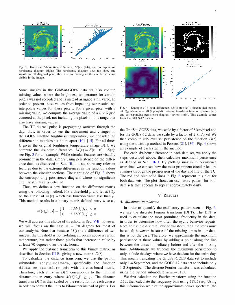
Fig. 3. Hurricane 6-hour time difference, M(t), (left), and correspondingpersistence diagram (right). The persistence diagram does not show anysignificant off diagonal point, thus it is not picking up the circular structurevisible in the image.

Some images in the GridSat-GOES data set also containmissing values where the brightness temperature for certainpixels was not recorded and is instead assigned a fill value. Inorder to prevent these values from impacting our results, weinterpolate values for these pixels. For a given pixel with amissing value, we compute the average value of a 5× 5 gridcentered at the pixel, not including the pixels in this range thatalso have missing values.

The TC diurnal pulse is propagating outward through theday; thus, in order to see the movement and changes inthe GOES satellite brightness temperature, we consider thedifference in matrices six hours apart [10], [15]. For all timest, given the original brightness temperature image S(t), wecompute the six-hour differences, M(t) = S(t+ 6)− S(t);see Fig. 3 for an example. While circular features are visuallyprominent in the data, simply using persistence on the differ-ence data, as discussed in Sec. III, did not show any relevantfeatures due to the extreme differences in the function valuesbetween the circular sections. The right side of Fig. 3 showsthe corresponding persistence diagram where no significantcircular structure is detected.

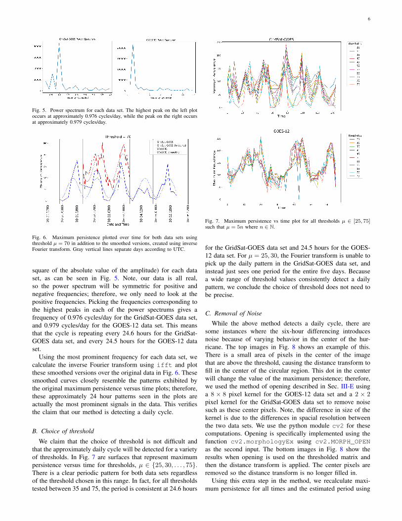
Thus, we define a new function on the difference matrixusing the following method. Fix a threshold µ and let M(t)µbe the subset of M(t) which has function value less than µ.This method results in a binary matrix defined entry-wise as,

M(t)µ[i, j] =

{1 if M(t)[i, j] < µ

0 if M(t)[i, j] ≥ µ.

We will address this choice of threshold in Sec. V-B; however,we will focus on the case µ = 70 degrees for most ofour analysis. Note that because M(t) is a difference of twoimages, the threshold is not isolating all pixels above a certaintemperature, but rather those pixels that increase in value byat least 70 degrees over the six hours.

We apply the distance transform to this binary matrix, asdescribed in Section III-B, giving a new matrix D(t).

To calculate the distance transform, we use the pythonsubmodule scipy.ndimage, specifically the functiondistance_transform_cdt with the chessboard metric.Therefore, each entry in D(t) corresponds to the minimaldistance to an entry where M(t)[i, j] ≥ µ. The distancetransform D(t) is then scaled by the resolution for each datasetin order to convert the units to kilometers instead of pixels. For

Fig. 4. Example of 6 hour difference, M(t) (top left), thresholded subset,M(t)µ where µ = 70 (top right), distance transform function (bottom left)and corresponding persistence diagram (bottom right). This example comesfrom the GOES-12 data set.

the GridSat-GOES data, we scale by a factor of 8 km/pixel andfor the GOES-12 data, we scale by a factor of 2 km/pixel Wethen compute sub-level set persistence on the function D(t)using the cubtop method in Perseus [21], [36]. Fig. 4 showsan example of each step in the method.

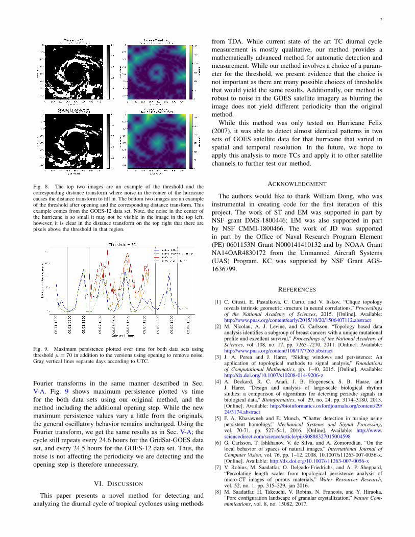
For each six-hour difference in each data set, we apply thesteps described above, then calculate maximum persistenceas defined in Sec. III-D. By plotting maximum persistenceover time, we can see how the most prominent circular featurechanges through the progression of the day and life of the TC.The red and blue solid lines in Fig. 6 represent this plot forboth data sets. The plot shows an oscillatory pattern for bothdata sets that appears to repeat approximately daily.

V. RESULTS

A. Maximum persistence

In order to quantify the oscillatory pattern seen in Fig. 6,we use the discrete Fourier transform (DFT). The DFT isused to calculate the most prominent frequency in the data,in order to determine how often the cyclic behavior repeats.Note, to use the discrete Fourier transform the time steps mustbe equal; however, because of the missing times in our data,this is not the case. Therefore, we approximate the maximumpersistence at these values by adding a point along the linebetween the times immediately before and after the missingtime. Additionally, we truncate the maximum persistence toonly include the days where we have the data for the entire day.This means truncating the GridSat-GOES data set to includeonly 1-4 September, and the GOES-12 data set to include only1-2 September. The discrete Fourier transform was calculatedusing the python submodule numpy.fft.

We first calculate the Fourier transform using the functionfft, then calculate the frequency bins using fftfreq. Usingthis information we plot the approximate power spectrum (the

6

Fig. 5. Power spectrum for each data set. The highest peak on the left plotoccurs at approximately 0.976 cycles/day, while the peak on the right occursat approximately 0.979 cycles/day.

Fig. 6. Maximum persistence plotted over time for both data sets usingthreshold µ = 70 in addition to the smoothed versions, created using inverseFourier transform. Gray vertical lines separate days according to UTC.

square of the absolute value of the amplitude) for each dataset, as can be seen in Fig. 5. Note, our data is all real,so the power spectrum will be symmetric for positive andnegative frequencies; therefore, we only need to look at thepositive frequencies. Picking the frequencies corresponding tothe highest peaks in each of the power spectrums gives afrequency of 0.976 cycles/day for the GridSat-GOES data set,and 0.979 cycles/day for the GOES-12 data set. This meansthat the cycle is repeating every 24.6 hours for the GridSat-GOES data set, and every 24.5 hours for the GOES-12 dataset.

Using the most prominent frequency for each data set, wecalculate the inverse Fourier transform using ifft and plotthese smoothed versions over the original data in Fig. 6. Thesesmoothed curves closely resemble the patterns exhibited bythe original maximum persistence versus time plots; therefore,these approximately 24 hour patterns seen in the plots areactually the most prominent signals in the data. This verifiesthe claim that our method is detecting a daily cycle.

B. Choice of threshold

We claim that the choice of threshold is not difficult andthat the approximately daily cycle will be detected for a varietyof thresholds. In Fig. 7 are surfaces that represent maximumpersistence versus time for thresholds, µ ∈ {25, 30, . . . , 75}.There is a clear periodic pattern for both data sets regardlessof the threshold chosen in this range. In fact, for all thresholdstested between 35 and 75, the period is consistent at 24.6 hours

Fig. 7. Maximum persistence vs time plot for all thresholds µ ∈ [25, 75]such that µ = 5n where n ∈ N.

for the GridSat-GOES data set and 24.5 hours for the GOES-12 data set. For µ = 25, 30, the Fourier transform is unable topick up the daily pattern in the GridSat-GOES data set, andinstead just sees one period for the entire five days. Becausea wide range of threshold values consistently detect a dailypattern, we conclude the choice of threshold does not need tobe precise.

C. Removal of Noise

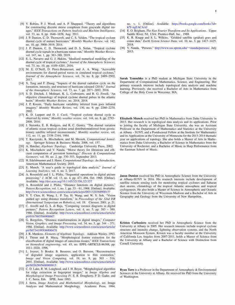
While the above method detects a daily cycle, there aresome instances where the six-hour differencing introducesnoise because of varying behavior in the center of the hur-ricane. The top images in Fig. 8 shows an example of this.There is a small area of pixels in the center of the imagethat are above the threshold, causing the distance transform tofill in the center of the circular region. This dot in the centerwill change the value of the maximum persistence; therefore,we used the method of opening described in Sec. III-E usinga 8 × 8 pixel kernel for the GOES-12 data set and a 2 × 2pixel kernel for the GridSat-GOES data set to remove noisesuch as these center pixels. Note, the difference in size of thekernel is due to the differences in spacial resolution betweenthe two data sets. We use the python module cv2 for thesecomputations. Opening is specifically implemented using thefunction cv2.morphologyEx using cv2.MORPH_OPENas the second input. The bottom images in Fig. 8 show theresults when opening is used on the thresholded matrix andthen the distance transform is applied. The center pixels areremoved so the distance transform is no longer filled in.

Using this extra step in the method, we recalculate maxi-mum persistence for all times and the estimated period using

7

Fig. 8. The top two images are an example of the threshold and thecorresponding distance transform where noise in the center of the hurricanecauses the distance transform to fill in. The bottom two images are an exampleof the threshold after opening and the corresponding distance transform. Thisexample comes from the GOES-12 data set. Note, the noise in the center ofthe hurricane is so small it may not be visible in the image in the top left;however, it is clear in the distance transform on the top right that there arepixels above the threshold in that region.

Fig. 9. Maximum persistence plotted over time for both data sets usingthreshold µ = 70 in addition to the versions using opening to remove noise.Gray vertical lines separate days according to UTC.

Fourier transforms in the same manner described in Sec.V-A. Fig. 9 shows maximum persistence plotted vs timefor the both data sets using our original method, and themethod including the additional opening step. While the newmaximum persistence values vary a little from the originals,the general oscillatory behavior remains unchanged. Using theFourier transform, we get the same results as in Sec. V-A; thecycle still repeats every 24.6 hours for the GridSat-GOES dataset, and every 24.5 hours for the GOES-12 data set. Thus, thenoise is not affecting the periodicity we are detecting and theopening step is therefore unnecessary.

VI. DISCUSSION

This paper presents a novel method for detecting andanalyzing the diurnal cycle of tropical cyclones using methods

from TDA. While current state of the art TC diurnal cyclemeasurement is mostly qualitative, our method provides amathematically advanced method for automatic detection andmeasurement. While our method involves a choice of a param-eter for the threshold, we present evidence that the choice isnot important as there are many possible choices of thresholdsthat would yield the same results. Additionally, our method isrobust to noise in the GOES satellite imagery as blurring theimage does not yield different periodicity than the originalmethod.

While this method was only tested on Hurricane Felix(2007), it was able to detect almost identical patterns in twosets of GOES satellite data for that hurricane that varied inspatial and temporal resolution. In the future, we hope toapply this analysis to more TCs and apply it to other satellitechannels to further test our method.

ACKNOWLEDGMENT

The authors would like to thank William Dong, who wasinstrumental in creating code for the first iteration of thisproject. The work of ST and EM was supported in part byNSF grant DMS-1800446; EM was also supported in partby NSF CMMI-1800466. The work of JD was supportedin part by the Office of Naval Research Program Element(PE) 0601153N Grant N000141410132 and by NOAA GrantNA14OAR4830172 from the Unmanned Aircraft Systems(UAS) Program. KC was supported by NSF Grant AGS-1636799.

REFERENCES

[1] C. Giusti, E. Pastalkova, C. Curto, and V. Itskov, “Clique topologyreveals intrinsic geometric structure in neural correlations,” Proceedingsof the National Academy of Sciences, 2015. [Online]. Available:http://www.pnas.org/content/early/2015/10/20/1506407112.abstract

[2] M. Nicolau, A. J. Levine, and G. Carlsson, “Topology based dataanalysis identifies a subgroup of breast cancers with a unique mutationalprofile and excellent survival,” Proceedings of the National Academy ofSciences, vol. 108, no. 17, pp. 7265–7270, 2011. [Online]. Available:http://www.pnas.org/content/108/17/7265.abstract

[3] J. A. Perea and J. Harer, “Sliding windows and persistence: Anapplication of topological methods to signal analysis,” Foundationsof Computational Mathematics, pp. 1–40, 2015. [Online]. Available:http://dx.doi.org/10.1007/s10208-014-9206-z

[4] A. Deckard, R. C. Anafi, J. B. Hogenesch, S. B. Haase, andJ. Harer, “Design and analysis of large-scale biological rhythmstudies: a comparison of algorithms for detecting periodic signals inbiological data,” Bioinformatics, vol. 29, no. 24, pp. 3174–3180, 2013.[Online]. Available: http://bioinformatics.oxfordjournals.org/content/29/24/3174.abstract

[5] F. A. Khasawneh and E. Munch, “Chatter detection in turning usingpersistent homology,” Mechanical Systems and Signal Processing,vol. 70-71, pp. 527–541, 2016. [Online]. Available: http://www.sciencedirect.com/science/article/pii/S0888327015004598

[6] G. Carlsson, T. Ishkhanov, V. de Silva, and A. Zomorodian, “On thelocal behavior of spaces of natural images,” International Journal ofComputer Vision, vol. 76, pp. 1–12, 2008, 10.1007/s11263-007-0056-x.[Online]. Available: http://dx.doi.org/10.1007/s11263-007-0056-x

[7] V. Robins, M. Saadatfar, O. Delgado-Friedrichs, and A. P. Sheppard,“Percolating length scales from topological persistence analysis ofmicro-CT images of porous materials,” Water Resources Research,vol. 52, no. 1, pp. 315–329, jan 2016.

[8] M. Saadatfar, H. Takeuchi, V. Robins, N. Francois, and Y. Hiraoka,“Pore configuration landscape of granular crystallization,” Nature Com-munications, vol. 8, no. 15082, 2017.

8

[9] V. Robins, P. J. Wood, and A. P. Sheppard, “Theory and algorithmsfor constructing discrete morse complexes from grayscale digital im-ages,” IEEE Transactions on Pattern Analysis and Machine Intelligence,vol. 33, no. 8, pp. 1646–1658, Aug. 2011.

[10] J. P. Dunion, C. D. Thorncroft, and C. S. Velden, “The tropical cyclonediurnal cycle of mature hurricanes,” Monthly Weather Review, vol. 142,no. 10, pp. 3900–3919, 2014.

[11] J. P. Dunion, C. D. Thorncroft, and D. S. Nolan, “Tropical cyclonediurnal cycle signals in a hurricane nature run,” Monthly Weather Review,vol. 147, no. 1, pp. 363–388, 2019.

[12] E. L. Navarro and G. J. Hakim, “Idealized numerical modeling of thediurnal cycle of tropical cyclones,” Journal of the Atmospheric Sciences,vol. 73, no. 10, pp. 4189–4201, 2016.

[13] M. E. O’Neill, D. Perez-Betancourt, and A. A. Wing, “Accessibleenvironments for diurnal-period waves in simulated tropical cyclones,”Journal of the Atmospheric Sciences, vol. 74, no. 8, pp. 2489–2502,2017.

[14] X. Tang and F. Zhang, “Impacts of the diurnal radiation cycle on theformation, intensity, and structure of hurricane edouard (2014),” Journalof the Atmospheric Sciences, vol. 73, no. 7, pp. 2871–2892, 2016.

[15] S. D. Ditchek, J. Molinari, K. L. Corbosiero, and R. G. Fovell, “Anobjective climatology of tropical cyclone diurnal pulses in the atlanticbasin,” Monthly Weather Review, no. 2018, 2018.

[16] J. P. Kossin, “Daily hurricane variability inferred from goes infraredimagery,” Monthly Weather Review, vol. 130, no. 9, pp. 2260–2270,2002.

[17] K. D. Leppert and D. J. Cecil, “Tropical cyclone diurnal cycle asobserved by trmm,” Monthly weather review, vol. 144, no. 8, pp. 2793–2808, 2016.

[18] J. Steranka, E. B. Rodgers, and R. C. Gentry, “The diurnal variationof atlantic ocean tropical cyclone aoud distributioninferred from geosta-tionary satellite infrared measurements,” Monthly weather review, vol.112, no. 11, pp. 2338–2344, 1984.

[19] T. Kaczynski, K. Mischaikow, and M. Mrozek, Computational homol-ogy. Springer Science & Business Media, 2006, vol. 157.

[20] A. Hatcher, Algebraic Topology. Cambridge University Press, 2002.[21] K. Mischaikow and V. Nanda, “Morse theory for filtrations and effi-

cient computation of persistent homology,” Discrete & ComputationalGeometry, vol. 50, no. 2, pp. 330–353, September 2013.

[22] H. Edelsbrunner and J. Harer, Computational Topology: An Introduction.American Mathematical Society, 2010.

[23] E. Munch, “A user’s guide to topological data analysis,” Journal ofLearning Analytics, vol. 4, no. 2, 2017.

[24] A. Rosenfeld and J. L. Pfaltz, “Sequential operations in digital pictureprocessing,” J. ACM, vol. 13, no. 4, pp. 471–494, Oct. 1966. [Online].Available: http://doi.acm.org/10.1145/321356.321357

[25] A. Rosenfeld and J. Pfaltz, “Distance functions on digital pictures,”Pattern Recognition, vol. 1, no. 1, pp. 33 – 61, 1968. [Online]. Available:http://www.sciencedirect.com/science/article/pii/0031320368900137

[26] Y. T. Chin, H. Wang, L. P. Tay, H. Wang, and W. Y. Soh, “Visionguided agv using distance transform,” in Proceedings of the 32nd ISR(International Symposium on Robotics), vol. 19. Citeseer, 2001, p. 21.

[27] C. Arcelli and G. S. di Baja, “Computing voronoi diagrams in digitalpictures,” Pattern Recognition Letters, vol. 4, no. 5, pp. 383 – 389,1986. [Online]. Available: http://www.sciencedirect.com/science/article/pii/0167865586900607

[28] G. Borgefors, “Distance transformations in digital images,” ComputerVision, Graphics, and Image Processing, vol. 34, no. 3, pp. 344 – 371,1986. [Online]. Available: http://www.sciencedirect.com/science/article/pii/S0734189X86800470

[29] J. R. Munkres, Elements of Algebraic Topology. Addison Wesley, 1993.[30] J. Thiran and B. Macq, “Morphological feature extraction for the

classification of digital images of cancerous tissues,” IEEE Transactionson biomedical engineering, vol. 43, no. EPFL-ARTICLE-86388, pp.1011–1020, 1996.

[31] L. Joyeux, S. Boukir, B. Besserer, and O. Buisson, “Reconstructionof degraded image sequences. application to film restoration,”Image and Vision Computing, vol. 19, no. 8, pp. 503 – 516,2001. [Online]. Available: http://www.sciencedirect.com/science/article/pii/S0262885600000913

[32] C. D. Lake, R. M. Lougheed, and J. H. Beyer, “Morphological algorithmfor ridge extraction in fingerprint images,” in Image Algebra andMorphological Image Processing IV, E. R. Dougherty, P. D. Gader, andJ. C. Serra, Eds. SPIE, June 1993.

[33] J. Serra, Image Analysis and Mathematical Morphology, ser. ImageAnalysis and Mathematical Morphology. Academic Press, 1984,

no. v. 1. [Online]. Available: https://books.google.com/books?id=kfY-ngEACAAJ

[34] E. O. Brigham, The Fast Fourier Transform and Its Applications. UpperSaddle River, NJ, USA: Prentice-Hall, Inc., 1988.

[35] K. R. Knapp and S. L. Wilkins, “Gridded satellite (gridsat) goes andconus data,” Earth System Science Data, vol. 10, no. 3, pp. 1417–1425,2018.

[36] V. Nanda, “Perseus,” http://www.sas.upenn.edu/∼vnanda/perseus/, July2015.

Sarah Tymochko is a PhD student at Michigan State University in theDepartment of Computational Mathematics, Science, and Engineering. Herprimary research interests include topological data analysis and machinelearning. Previously, she received a Bachelor of Arts in Mathematics fromCollege of the Holy Cross in Worcester, MA.

Elizabeth Munch received her PhD in Mathematics from Duke University in2013. Her research is in topological data analysis and its applications. Priorto joining the faculty of Michigan State University, she was an AssistantProfessor in the Department of Mathematics and Statistics at the Universityat Albany - SUNY, and a Postdoctoral Fellow at the Institute for Mathematicsand its Applications at the University of Minnesota for the 2013-2014 thematicyear on applications of topology. She also holds a Master of Arts in Mathe-matics from Duke University, a Bachelor of Science in Mathematics from theUniversity of Rochester, and a Bachelor of Music in Harp Performance fromthe Eastman School of Music.

Jason Dunion received his PhD in Atmospheric Science from the Universityat Albany-SUNY in 2016. His research interests include development ofsatellite remote sensing tools for monitoring tropical cyclones and Saharandust storms, climatology of the tropical Atlantic atmosphere and tropicalcyclogenesis. He also holds a Master of Science in Atmospheric and OceanicScience from the University of Wisconsin-Madison and a Bachelor of Arts inGeography and Geology from the University of New Hampshire.

Kristen Corbosiero received her PhD in Atmospheric Science from theUniversity at Albany in 2005. Her research interests include tropical cyclonestructure and intensity change, lightning observation systems, and the NorthAmerican Monsoon System. Kristen was a faculty member at the Universityof California Los Angeles from 2007-2011, holds a Master of Science fromthe University at Albany and a Bachelor of Science with Distinction fromCornell University.

Ryan Torn is a Professor in the Department of Atmospheric & EnvironmentalSciences at the University at Albany. He received his PhD from the Universityof Washington.