using pivot tables - the document foundation€¦ · using pivot tables, you can view different...

Calc Guide

Chapter 8 Using Pivot Tables

Copyright

This document is Copyright © 2009–2012 by its contributors as listed below. You may distribute it and/or modify it under the terms of the Creative Commons Attribution-Share Alike License (http://creativecommons.org/licenses/by-sa/3.0/), version 3.0 or later.

All trademarks within this guide belong to their legitimate owners.

AuthorsBarbara DupreyMartin J FoxJean Hollis WeberJohn A Smith

FeedbackPlease direct any comments or suggestions about this document to: [email protected]

AcknowledgmentsThis chapter is based on and updated from Chapter 8 of the OpenOffice.org 3.3 Calc Guide, which was adapted from a German original written by Stefan Weigel and translated into English by Sigrid Kronenberger. Other contributors to that chapter are:

Jean Hollis Weber Andy Brown Sharon WhistonClaire Wood Martin Fox

Publication date and software versionPublished 17 July 2012. Based on LibreOffice 3.4.6.

Note for Mac users

Some keystrokes and menu items are different on a Mac from those used in Windows and Linux. The table below gives some common substitutions for the instructions in this chapter. For a more detailed list, see the application Help.

Windows or Linux Mac equivalent Effect

Tools > Options menu selection

LibreOffice > Preferences Access setup options

Right-click Control+click Opens a context menu

Ctrl (Control) z (Command) Used with other keys

F5 Shift+z+F5 Opens the Navigator

F11 z+T Opens the Styles and Formatting window

Documentation for LibreOffice is available at http://www.libreoffice.org/get-help/documentation

http://www.libreoffice.org/get-help/documentation

mailto:[email protected]

http://creativecommons.org/licenses/by-sa/3.0/

Contents

Copyright.............................................................................................................................. 2

Note for Mac users...............................................................................................................2

Important note...................................................................................................................... 4

Introduction.......................................................................................................................... 4Database preconditions............................................................................................................... 4

Data sources................................................................................................................................5Calc spreadsheet.................................................................................................................... 5Registered data source........................................................................................................... 5

Creating a Pivot Table.................................................................................................................. 6

The DataPilot dialog.............................................................................................................6Basic layout................................................................................................................................. 6

More options................................................................................................................................ 8

More settings for the fields: Field options................................................................................... 10Options for Data Fields..........................................................................................................10Options for Row and Column Fields...................................................................................... 12Options for Page Fields......................................................................................................... 15

Working with the results of the DataPilot (the Pivot Table)...........................................15Changing the layout................................................................................................................... 15

Grouping rows or columns......................................................................................................... 15

Grouping of categories with scalar values..................................................................................16

Grouping without automatic creation of intervals....................................................................... 17

Sorting the result........................................................................................................................ 18Select sort order from drop-down menus on each column heading.......................................18Sort manually by using drag and drop................................................................................... 19Sort automatically.................................................................................................................. 19

Drilling (showing details)............................................................................................................ 20

Filtering...................................................................................................................................... 22

Updating (refreshing) changed values....................................................................................... 23

Cell formatting............................................................................................................................ 23

Using shortcuts.......................................................................................................................... 23

Using Pivot Table results elsewhere................................................................................23The problem............................................................................................................................... 23

The solution: Function GETPIVOTDATA.................................................................................... 24Syntax................................................................................................................................... 24First syntax variation............................................................................................................. 25Second syntax variation........................................................................................................ 25

Using Pivot Tables 3

Important note

Unfortunately, due to the complexities of modern software, the Pivot Table function is incompletely implemented in this release (v3.4) of Calc.

• The Group and Outline functionality for any time interval is not available.

• The DataPilot dialog should have been renamed to Pivot Table to match the parent function, but this was not done.

If you wish to use this function to its full extent, we strongly recommend that that you upgrade to LibreOffice version 3.5, which fully implements Pivot Table’s functionality.

Introduction

Many requests for software support are the result of using complicated formulas and solutions to solve simple day to day problems. More efficient and effective solutions use the Pivot Table, a tool for combining, comparing, and analyzing large amounts of data easily. Using Pivot Tables, you can view different summaries of the source data, display the details of areas of interest, and create reports, whether you are a beginner, an intermediate or advanced user.

Database preconditionsThe first thing needed to work with the Pivot Table is a list of raw data, similar to a database table, consisting of rows (data sets) and columns (data fields). The field names are in the first row above the list.

The data source could be an external file or database. For the simplest case, where data is contained in a Calc spreadsheet, Calc offers sorting functions that do not require the Pivot Table.

For processing data in lists, the program needs to know where in the spreadsheet the table is. The table can be anywhere in the sheet, in any position. A spreadsheet can contains several unrelated tables.

Calc recognizes your lists automatically. It uses the following logic: Starting from the cell you’ve selected (which must be within your list), Calc checks the surrounding cells in all 4 directions (left, right, above, below). The border is recognized if the program discovers an empty row or column, or if it hits the left or upper border of the spreadsheet.

This means that the described functions can only work correctly if there are no empty rows or columns in your list. Avoid empty lines (for example for formatting). You can format your list by using cell formats.

Rule No empty rows or empty columns are allowed within lists.

If you select more than one single cell before you start sorting, filtering or calling the Pivot Table, then the automatic list recognition is switched off. Calc assumes that the list matches exactly the cells you have selected.

Rule For sorting, filtering, or using the Pivot Table, always select only one cell.

A relatively common source of errors is to inadvertently declare a list by mistake and then sort the list. If you select multiple cells (for example, a whole column) then the sorting mixes up the data that should be together in one row.

In addition to these formal aspects, the logical structure of your table is very important when using the Pivot Table.

4 Using Pivot Tables

RuleCalc lists must have the normal form; that is, they must have a simple linear structure.

When entering the data, do not add outlines, groups, or summaries. Here are some mistakes commonly made by inexperienced spreadsheet users:

1) You made several sheets, for example, a sheet for each group of articles. Analyses are then possible only within each group. Analyses for several groups would be a lot of work.

2) In the Sales list, instead of only one column for the amount, you made a column for the amounts for each employee. The amounts then had to be entered into the appropriate column. An analysis with the Pivot Table would not be possible any more. In contrast, one result of the Pivot Table is that you can get results for each employee if you have entered everything in one column.

3) You entered the amounts in chronological order. At the end of each month you made a sum total. In this case, sorting the list for different criteria is not possible because the Pivot Table will treat the sum totals the same as any other figure. Getting monthly results is one of the very fast and easy features of the Pivot Table.

Data sourcesAt this time, the possible data sources for the Pivot Table are a Calc spreadsheet or an external data source that has to be registered in LibreOffice.

Calc spreadsheetThe simplest and most often used case is analyzing a list in a Calc spreadsheet. The list might be updated regularly or the data might be imported from a different application.

For example, a list can be copied from a different application and pasted into Calc. The behavior of Calc while inserting the data depends on the format of the data. If the data is in a common spreadsheet format, it is copied directly into Calc. However, if the data is in plain text, the Text Import dialog (Figure 1) appears after you select the file containing the data; see Chapter 1, Introducing Calc, for more more information about this dialog.

Calc can import data from a huge number of foreign data formats, for example from other spreadsheets (Excel, Lotus 1, 2, 3), from databases (like dBase), and from simple text files including CSV formats.

The drawback of copying or importing foreign data is that it will not update automatically if there are changes in the source file. With a Calc file you were previously limited to 65,535 rows but this has been expanded to 1,048,576 rows.

Registered data sourceA registered data source in LibreOffice is a connection to data held in a database outside Calc. This means that the data to be analyzed will not be saved in Calc; Calc always uses the data from the original source. Calc is able to use many different data sources and also databases that are created and maintained with LibreOffice Base. See Chapter 10, Linking Calc Data, for more information.

Introduction 5

Figure 1: Import settings

Creating a Pivot TableCreate the Pivot Table using Data > Pivot Table > Create from the menu bar. If the list to be analyzed is in a spreadsheet table, select only one cell within this list. Calc recognizes and selects the list automatically for use with the Pivot Table (Figure 2).

The DataPilot dialog

The function of the Pivot Table is managed in two places: first in the DataPilot dialog and second through manipulations of the result in the spreadsheet. This section describes the dialog in detail.

Basic layoutIn the DataPilot dialog (Figure 3) are four white areas that show the layout of the result. Beside these white areas are buttons with the names of the fields in your data source. To choose a layout, drag and drop the field buttons into the white areas.

The Data Fields area in the middle must contain at least one field. Advanced users can use more than one field here. For the Data Field an aggregate function is used. For example, if you move the sales field into the Data Fields area, it appears there as Sum – sales.


Figure 2: After starting the Pivot Table

Figure 3: DataPilot dialog

Row Fields and Column Fields indicate from which groups the result will be sorted. Often more than one field is used at a time to get partial sums for rows or columns. The order of the fields gives the order of the sums from overall to specific.

For example, if you drag region and employee into the Row Fields area, the sum will be divided into the employees. Within the employees will be the listing for the different regions (see Figure 4).

The DataPilot dialog 7

Figure 4: DataPilot field order for analysis, and resulting layout in pivot table

Fields that are placed into the Page Fields area appear in the result above as a drop down list. The summary in your result takes only that part of your base data into account that you have selected. For example, if you use employee as a Page Field, you can filter the result shown for each employee.

To remove a field from the white layout area, just drag it past the border and drop it (the cursor will change to a crossed symbol), or select it and click the Remove button.

More optionsTo expand the DataPilot dialog and show more options, click More.

Figure 5: Expanded dialog of the DataPilot

Selection fromShows the sheet name and the range of cells used for the Pivot Table.

Results toResults to defines where your result will be shown. Selecting Results to as – undefined – and entering a cell reference tells the Pivot Table where to show the results.1 An error dialog is displayed if you fail to enter a cell reference. Selecting Results to as - new sheet – adds a new sheet to the spreadsheet file and places the results there. The new sheet is named using the format Pivot Table_sheet name_X; where X is the number of the table created, 1 for first, 2 for second and so on. For the source shown in Figure 3, the new sheet for the first table produced, would be named Pivot Table_Umsatzliste_1. Each new sheet is inserted next to the source sheet.

Ignore empty rowsIf the source data is not in the recommended form, this option tells the Pivot Table to ignore empty rows.

1 In this case the word - undefined – is misleading because the output position is in fact defined.


Identify categoriesWith this option selected, if the source data has missing entries in a list and does not meet the recommended data structure (see Figure 6), the Pivot Table adds it to the listed category above it. If this option is not chosen, then the Pivot Table inserts (empty) (see Figure 8).

Figure 6: Example of data with missing entries in Column A

The option Identify categories ensures that in this example rows 3 and 4 are included for the product Apples and row 6 is included for Pears (see Figure 7).

Figure 7: Pivot Table result with Identify categories selected

Without category recognition, the DataPilot shows an (empty) category (Figure 8).

Figure 8: Pivot Table result without Identify categories selected

Logically, the behavior with category recognition is better. A list showing missing entries is also less useful, because you cannot use functions such as sorting or filtering.

Total columns, Total rowsWith these options you can decide if the Pivot Table shows an extra row with the sums of each column, or if it adds on the very right a column with the sums of each row. In some cases, an added total sum is meaningless, for example if your entries are accumulated or the result of comparisons.

Add filterUse this option to add or hide the cell labeled Filter above the Pivot Table results. This cell is a convenient button for additional filtering options within the Pivot Table.

Enable drill to detailsWith this option enabled, if you double-click on a single data cell, including a cell produced from Total columns or Total rows, in the Pivot Table result, a new sheet opens giving a detailed listing of the individual entry. If you double-click on either a cell in the Row Fields, or Column Fields, then the Show Detail dialog opens (see “Drilling (showing details)” on page 20). Taking Figure 4 as an example, if a pivot table uses more than one field (region and employee) and you double-click a left-most field (say, east), then this collapses the row, combining the totals


for employees for that field and displaying the totals for east. If this function is disabled, the double-click will keep its usual edit function within a spreadsheet.

More settings for the fields: Field optionsThe options discussed in the previous section are valid for the DataPilot in general. You can also change settings for every field that you have added to the DataPilot layout. Do this either by selecting a field and clicking on the Options button in the DataPilot dialog, or by double-clicking on the appropriate field.

The options available for fields put into the Data Fields differ from those put into the Row, Column, and Page Fields of the DataPilot.

Options for Data FieldsIn the Options dialog of a Data Field you can select the Sum function for accumulating the values from your data source. You will often use the sum function, but other functions (like standard distribution or a counting function) are also available. For example, the counting function can be useful for non-numerical data fields.

On the Data Field dialog, click More to see the Displayed value section.

Figure 9: Expanded dialog for a Data Field

In the Displayed value section, you can choose other possibilities for analysis by using the aggregate function. Depending on the setting for Type, you may have to choose definitions for Base field and Base item.

Figure 10: Example choices for Base field and item


The table below lists the possible types of displayed value and associated base field and item, together with a note on usage.

Type Base field Base item Analysis

Normal — — Simple use of the chosen aggregate function (for example, sum).

Difference from

Selection of a field from the data source of the DataPilot (for example, employee).

Selection of an element from the selected base field (for example, Brigitte).

The result is the difference between the result of the Base field and the Base item (for example, sales volume of the employees against the sales volume of Brigitte; see Figure 11).

% of Selection of a field from the data source of the DataPilot (for example, employee)

Selection of an element from the selected base field (for example, Brigitte)

The result is a percentage ratio of the value of the base field to the base item (for example, sales result of the employee relative to the sales result of Brigitte; see Figure 12).

% difference from

Selection of a field from the data source of the DataPilot (for example, employee)

Selection of an element from the selected base field (for example. Brigitte)

From each result, its reference value is subtracted, and the difference is divided by the reference value (for example, sales of the employees as relative difference from the sales of Brigitte; see Figure 13).

Running total in

Selection of a field from the data source of the DataPilot (for example, date)

— Each result is added to the sum of the results for preceding items in the base field, in the base field’s sort order, and the total sum is shown.

Results are always summed, even if a different summary function was used to get each result.

% of row — — The result is a percentage of the value of the whole row (for example, the row sum).

% of column

— — The result is a percentage of the total column value (for example, the column sum).

% of total — — The result is a percentage of the overall result (for example, the total sum).

Index — — (Default result x total result) / (row total x column total)


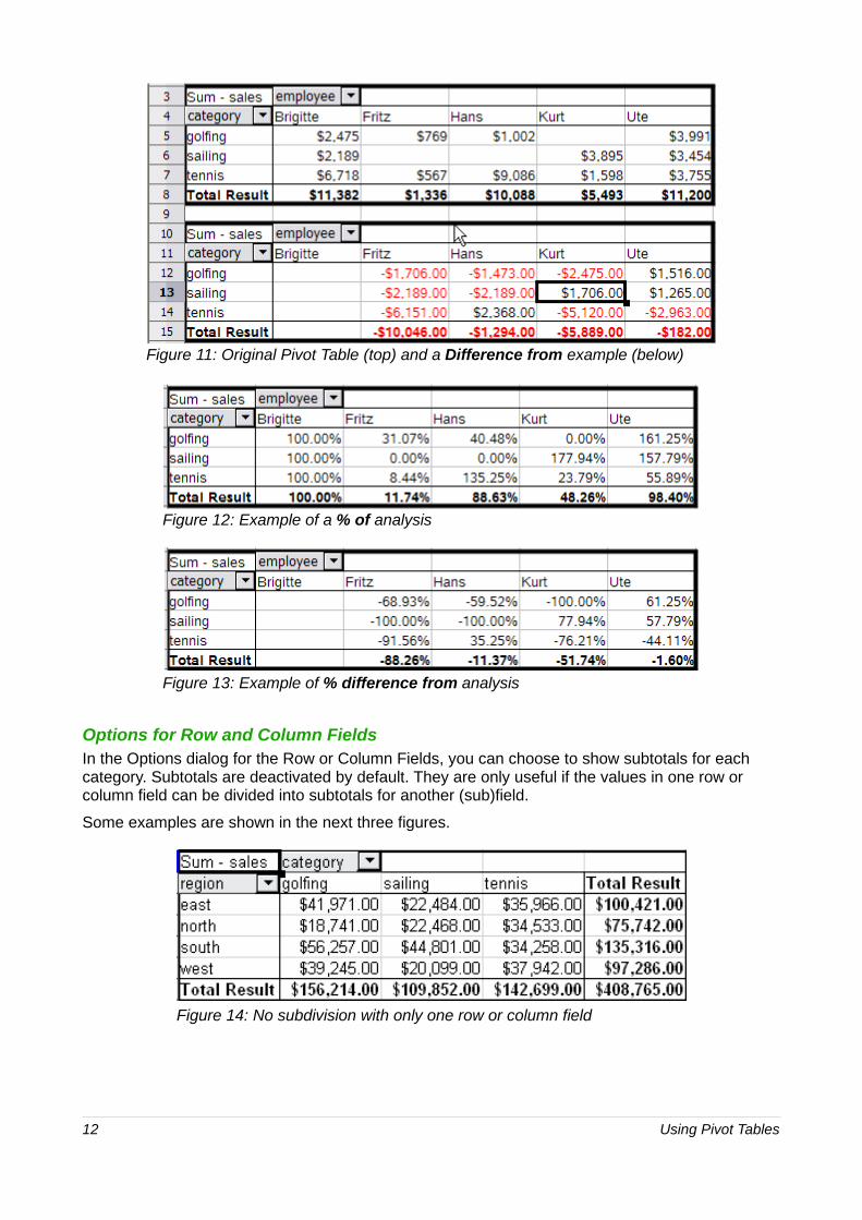
Figure 11: Original Pivot Table (top) and a Difference from example (below)

Figure 12: Example of a % of analysis

Figure 13: Example of % difference from analysis

Options for Row and Column FieldsIn the Options dialog for the Row or Column Fields, you can choose to show subtotals for each category. Subtotals are deactivated by default. They are only useful if the values in one row or column field can be divided into subtotals for another (sub)field.

Some examples are shown in the next three figures.

Figure 14: No subdivision with only one row or column field


Figure 15: Division of the regions for employees (two row fields) without subtotals

Figure 16: Division of the regions for employees with subtotals (by region)


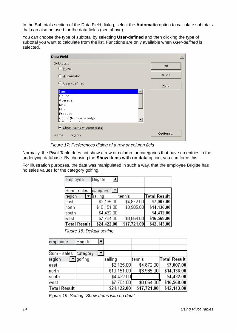
In the Subtotals section of the Data Field dialog, select the Automatic option to calculate subtotals that can also be used for the data fields (see above).

You can choose the type of subtotal by selecting User-defined and then clicking the type of subtotal you want to calculate from the list. Functions are only available when User-defined is selected.

Figure 17: Preferences dialog of a row or column field

Normally, the Pivot Table does not show a row or column for categories that have no entries in the underlying database. By choosing the Show items with no data option, you can force this.

For illustration purposes, the data was manipulated in such a way, that the employee Brigitte has no sales values for the category golfing.

Figure 18: Default setting

Figure 19: Setting “Show Items with no data”


Options for Page FieldsThe Options dialog for Page Fields is the same as for Row and Column fields, even though it appears to be useless to have the same settings as described for the Row and Column fields. With the flexibility of the DataPilot you can switch the different fields between pages, columns or rows. The fields keep the settings that you made for them. The Page Field has the same properties as a Row or Column field. These settings only take effect when you use the field not as a Page Field but as Row or Column field.

Working with the results of the DataPilot (the Pivot Table)

As mentioned above, the DataPilot dialog is very flexible. An analysis, a Pivot Table, can be totally restructured with only a few mouse clicks. Some functions of the DataPilot dialog can only be used with the Pivot Table.

Changing the layoutThe layout of the Pivot Table can be changed quickly and easily by drag and drop. With the DataPilot open, fields can be dragged around from row, column, page and the Data Fields areas to any position you want to put them, and then dropped. Unused fields can be added, and fields removed in error can be replaced by dragging and dropping them into the positions required.

Some manipulation can also be carried out in the pivot table view. Within the results table of the Pivot Table, move one of the page, column, or row fields to a different position. The cursor will change shape from its starting shape (horizontal or vertical block on the arrow head) to the opposite if moving to a different field, such as from row to column, and it is OK to drop.

Figure 20: Drag a column field. Note the cursor shape

Figure 21: Drag a row field. Note the cursor shape

You can remove a column, row, or page field from the Pivot Table by clicking on it and dragging it out of the table. The cursor changes to that shown in Figure 22. A field removed in error cannot be recovered and it is necessary to return to the DataPilot to replace it.

Figure 22: Field dragged out of the pivot table

Grouping rows or columnsFor many analyses or summaries, the categories have to be grouped. You can merge the results in classes. You can only carry out grouping on an ungrouped Pivot Table.

You can access grouping by selecting Data > Group and Outline > Group from the menu bar, or by pressing F12 after selecting the correct cell area. How the grouping function works is

Working with the results of the DataPilot (the Pivot Table) 15

determined mainly by the type of values that have to be grouped. You need to distinguish between scalar values, or other values, such as text, that you want grouped.

Date and time values can not be grouped in this release of Calc (see “Important note” on page 4).

Note

Before you can group, you have to produce a Pivot Table with ungrouped data. The time needed for creating a Pivot Table depends mostly on the number of columns and rows and not on the size of the basic data. Through grouping you can produce the Pivot Table with a small number of rows and columns. The Pivot Table can contain a lot of categories, depending on your data source.

Grouping of categories with scalar valuesFor grouping scalar values, select a single cell in the row or column of the category to be grouped.

Figure 23: Pivot Table without grouping (frequency of the km/h values of a radar control)

Figure 24: Pivot Table with grouping (classes of 10 km/h each)

Choose Data > Group and Outline > Group from the menu bar or press F12; you get the following dialog.

Figure 25: Grouping dialog with scalar categories


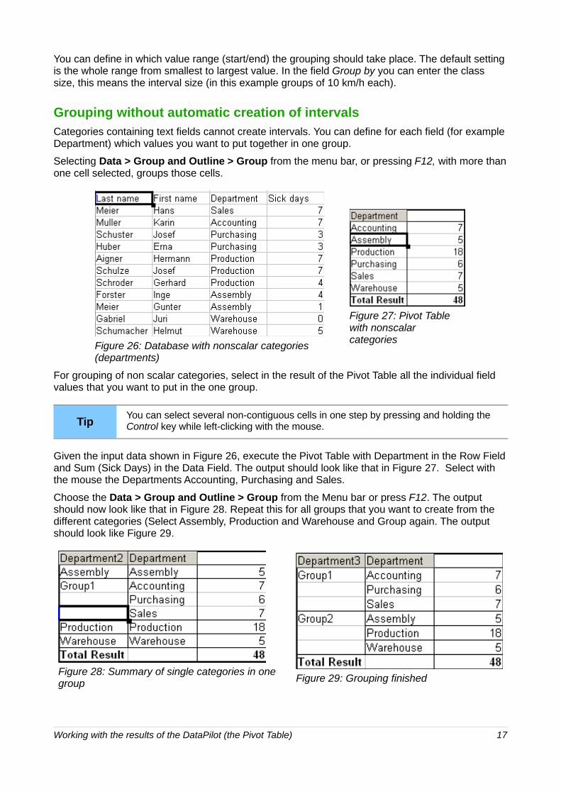
You can define in which value range (start/end) the grouping should take place. The default setting is the whole range from smallest to largest value. In the field Group by you can enter the class size, this means the interval size (in this example groups of 10 km/h each).

Grouping without automatic creation of intervalsCategories containing text fields cannot create intervals. You can define for each field (for example Department) which values you want to put together in one group.

Selecting Data > Group and Outline > Group from the menu bar, or pressing F12, with more than one cell selected, groups those cells.

Figure 26: Database with nonscalar categories (departments)

Figure 27: Pivot Table with nonscalar categories

For grouping of non scalar categories, select in the result of the Pivot Table all the individual field values that you want to put in the one group.

TipYou can select several non-contiguous cells in one step by pressing and holding the Control key while left-clicking with the mouse.

Given the input data shown in Figure 26, execute the Pivot Table with Department in the Row Field and Sum (Sick Days) in the Data Field. The output should look like that in Figure 27. Select with the mouse the Departments Accounting, Purchasing and Sales.

Choose the Data > Group and Outline > Group from the Menu bar or press F12. The output should now look like that in Figure 28. Repeat this for all groups that you want to create from the different categories (Select Assembly, Production and Warehouse and Group again. The output should look like Figure 29.

Figure 28: Summary of single categories in one group Figure 29: Grouping finished


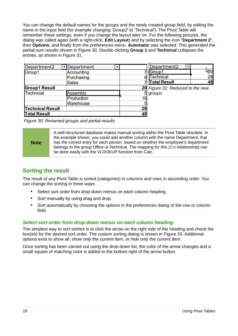
You can change the default names for the groups and the newly created group field, by editing the name in the input field (for example changing 'Group2' to 'Technical'). The Pivot Table will remember these settings, even if you change the layout later on. For the following pictures, the dialog was called again (with a right-click, Edit Layout) and by selecting the icon “Department 2”, then Options, and finally from the preferences menu Automatic was selected. This generated the partial sum results shown in Figure 30. Double clicking Group 1 and Technical collapses the entries, as shown in Figure 31.

Figure 30: Renamed groups and partial results

Figure 31: Reduced to the new groups

Note

A well-structured database makes manual sorting within the Pivot Table obsolete. In the example shown, you could add another column with the name Department, that has the correct entry for each person based on whether the employee’s department belongs to the group Office or Technical. The mapping for this (1:n relationship) can be done easily with the VLOOKUP function from Calc.

Sorting the resultThe result of any Pivot Table is sorted (categories) in columns and rows in ascending order. You can change the sorting in three ways:

• Select sort order from drop-down menus on each column heading.

• Sort manually by using drag and drop.

• Sort automatically by choosing the options in the preferences dialog of the row or column field.

Select sort order from drop-down menus on each column headingThe simplest way to sort entries is to click the arrow on the right side of the heading and check the box(es) for the desired sort order. The custom sorting dialog is shown in Figure 33. Additional options exist to show all, show only the current item, or hide only the current item.

Once sorting has been carried out using the drop-down list, the color of the arrow changes and a small square of matching color is added to the bottom right of the arrow button.


Figure 32: Arrow color change and indicator square on button

Figure 33: Custom sorting

Sort manually by using drag and dropYou can change the order within the categories by moving the cells with the category values in the result table of the Pivot Table. The cell will be inserted above the cell on which you drop it.

Be aware that in Calc a cell must be selected. It is not enough that this cell contains the cell cursor. The background of a selected cell is marked with a different color. To achieve this, click in one cell with no extra key pressed and redo this by pressing also the Shift or Ctrl key. Another possibility is to keep the mouse button pressed on the cell you want to select, move the mouse to a neighbor cell and move back to your original cell before you release the mouse button.

Sort automaticallyTo sort automatically, right-click within the Pivot Table and choose Edit Layout, to open the DataPilot (Figure 3). Within the Layout area of the DataPilot, double-click the row or column field you want to sort. In the Data Field dialog which opens (Figure 17), click Options to display the Data Field Options dialog.

For Sort by choose either Ascending or Descending. On the left side is a drop-down list where you can choose the field this setting should apply to. With this method you can specify that sorting does not happen according to the categories but according to the results of the data field.


Figure 34: Options for a row or column field

Drilling (showing details)Drill allows you to show the related detailed data for a single, compressed value in the Pivot Table result. To activate a drill, double-click on the cell or choose Data > Group and Outline > Show Details. There are two possibilities:

1) The active cell is a row or column field.

In this case, drill means an additional breakdown into the categories of another field.

For example, double-click on the cell with the value golfing. In this instance the values that are aggregated within golfing can be subdivided using another field.

Figure 35: Before the drill down for the category golfing

A dialog appears allowing you to select the field to use for further subdivision. In this example, employee.


Figure 36: Selecting the field for the subdivision

Figure 37: After the drill down

To hide the details again, double-click on the cell golfing or choose Data > Group and Outline > Hide Details.

The Pivot Table remembers your selection (in our example the field employee) by adding and hiding the selected field, so that for the next drill down for a category in the field category the dialog does not appear. To remove the selection employee, open the DataPilot dialog by right-clicking and choosing Edit Layout, then delete the unwanted selection in the row or column field.

2) The active cell is a value of the Data Field.

In this case, drill down results in a listing of all data entries of the data source that aggregates to this value.

In our example, if we were to double-click on the cell with the value $18,741 from Figure 35, we would now have a new list of all data sets that are included in this value. This list is displayed in a new sheet.


Figure 38: New table sheet after the drill down for a value in a data field

FilteringTo limit the Pivot Table analysis to a subset of the information that is contained in the data basis, you can filter with the Pivot Table.

NoteAn Autofilter or default filter used on the sheet has no effect on the DataPilot analysis process. The DataPilot always uses the complete list that was selected when it was started.

To do this, click Filter on the top left side above the results.

Figure 39: Filter field in the upper left area of the Pivot Table

In the Filter dialog, you can define up to 3 filter options that are used in the same way as Calc’s default filter.

Figure 40: Dialog for defining the filter

NoteEven if they are not called a filter, page fields are a practical way to filter the results. The advantage is that the filtering criteria used are clearly visible.


Updating (refreshing) changed valuesAfter you have created the Pivot Table, changes in the source data do not cause an automatic update in the resulting table. You must update (refresh) the Pivot Table manually after changing any of the underlying data values.

Changes in the source data could appear in two ways:

1) The content of existing data sets has been changed.

For example, you might have changed a sales value afterward. To update the Pivot Table, right-click in the result area and choose Refresh (or choose Data > Pivot Table > Refresh from the menu bar).

2) You have added or deleted data sets in the original list.

In this case the change means that the Pivot Table has to use a different area of the spreadsheet for its analysis. Fundamental changes to the data set collection means you must redo the Pivot Table from the beginning.

Cell formattingThe cells in the results area of the Pivot Table are automatically formatted in a simple format by Calc. You can change this formatting using all the tools in Calc, but note that if you make any change in the design of the Pivot Table or any updates, the formatting will return to the format applied automatically by Calc.

For the number format in the data field, Calc uses the number format that is used in the corresponding cell in the source list. In most cases, this is useful (for example, if the values are in the currency format, then the corresponding cell in the result area is also formatted as currency). However, if the result is a fraction or a percentage, the Pivot Table does not recognize that this might be a problem; such results must either be without a unit or be displayed as a percentage. Although you can correct the number format manually, the correction stays in effect only until the next update.

Using shortcutsIf you use the Pivot Table very often, you might find the frequent use of the menu paths (Data > Pivot Table > Create and Data > Group and Outline > Group) inconvenient.

For grouping, a shortcut is already defined: F12. For starting the Pivot Table, you can define your own keyboard shortcut. If you prefer to have toolbar icons instead of keyboard shortcuts, you can create a user-defined symbol and add it to either your own custom made toolbar or the Standard toolbar.

For an explanation how to create keyboard shortcuts or add icons to toolbars, see Chapter 14, Setting Up and Customizing Calc.

Using Pivot Table results elsewhere

The problemNormally you create a reference to a value by entering the address of the cell that contains the value. For example, the formula =C6*2 creates a reference to cell C6 and returns the doubled value.

If this cell is located in the results area of the Pivot Table, it contains the result that was calculated by referencing specific categories of the row and column fields. In Figure 41, the cell C6 contains the sum of the sales values of the employee Hans in the category Sailing. The formula in the cell C12 uses this value.

Using Pivot Table results elsewhere 23

Figure 41: Formula reference to a cell of the Pivot Table

If the underlying data or the layout of the Pivot Table changes, then you must take into account that the sales value for Hans might appear in a different cell. Your formula still references the cell C6 and therefore uses a wrong value. The correct value is in a different location. For example, in Figure 42, the location is now C7.

Figure 42: The value that you really want to use can be found now in a different location.

The solution: Function GETPIVOTDATAUse the function GETPIVOTDATA to have a reference to a value inside the Pivot Table by using the specific identifying categories for this value. This function can be used with formulas in Calc if you want to reuse the results from the Pivot Table elsewhere in your spreadsheet.

SyntaxThe syntax has two variations:

GETPIVOTDATA(target field, Pivot Table, [ Field name / Element, ... ])

GETPIVOTDATA(Pivot Table, specification)


First syntax variationThe target field specifies which data field of the Pivot Table is used within the function. If your Pivot Table has only one data field, this entry is ignored, but you must enter it anyway.

If your Pivot Table has more than one data field, then you have to enter the field name from the underlying data source (for example “sales”) or the field name of the data field itself (for example “sum – sales”).

The argument Pivot Table specifies the Pivot Table that you want to use. It is possible that your document contains more than one Pivot Table. Enter here a cell reference that is inside the area of your Pivot Table. It might be a good idea to always use the upper left corner cell of your Pivot Table, so you can be sure that the cell will always be within your Pivot Table, even if the layout changes.

Example: GETPIVOTDATA("sales",A1)

If you enter only the first two arguments, then the function returns the total result of the Pivot Table (“Sum – sales” entered as the field, will return a value of 408,765).

You can add more arguments as pairs with field name and item to retrieve specific partial sums. In the example in Figure 41, where we want to get the partial sum of Hans for sailing, the formula in cell C12 would look like this:

=GETPIVOTDATA("sales",A1,"employee","Hans","category","sailing")

Figure 43: First syntax variation

Second syntax variationThe argument Pivot Table has to be given in the same way as for the first syntax variation.

For the specifications, enter a list separated by spaces to specify the value you want from the Pivot Table. This list must contain the name of the data field, if there is more than one data field; otherwise it is not required. To select a specific partial result, add more entries in the form of Field name[item].

In the example in Figure 41, where we want to get the partial sum of Hans for Sailing, the formula in cell C12 would look like this:

=GETPIVOTDATA(A1,"sales employee[Hans] category[sailing]")

Using Pivot Table results elsewhere 25

Figure 44: Second syntax variation

When working with data sets containing date information, you must take care if you use the date information in the GETPIVOTDATA function. The function will only recognize the date entry if it is entered into the formula in exactly the same way that it appears in the data set from which the pivot table is produced. In the example of Figure 45, an error is returned when the date format does not match that of the data. Only with the correct format is the result returned.

Figure 45: Error produced if date information is not entered in correctly


using pivot tables - the document foundation€¦ · using pivot tables, you can view different...

Documents