using process simulation to predict wastewater treatment …dustin/spwccpaper3.pdf · lastly, it...

Using Process Simulation to Predict Wastewater Treatment

Outcomes

Dustin K. James, Ph.D.1 and Anthony J. Gerbino, Ph.D.2

1Chemistry and Technology Manager, Koch Microelectronic Service Co. Inc.

20 East Greenway Plaza, Houston, Texas 77046

Phone: (713) 544-5898 Fax: (713) 544-9086; E-mail: [email protected] 2Principal, Aqueous Process Simulations, Inc.

37 Herman Street, Glenn Ridge, New Jersey 07028

Phone: (973) 748-3352 Fax: (973) 748-5172; E-mail: [email protected]

Abstract

Changes occur rapidly in the semiconductor industry. New tools, new processes and the need to

increase process capacity greatly impact downstream activities, notably wastewater treatment.

The ability to predict how process changes affect water treatment will help to drive better

wastewater handling methods, as critical areas of concern are identified aprioi. This paper

examines the outcome of four waste treatment applications designed on the computer using real-

solution aqueous process simulation.

First, two typical fluoride waste water streams were treated with either Ca(OH)2 or CaCl2.

Process simulation was used to predict the chemical addition rate, and the clean water

composition following CaF2 removal. The predictions favorably compared to results achieved in

the lab on synthetic wastewater samples; differences were attributed to limitations in the lab

experimental procedures. Next, the effect of neutralization on dilute acid waste composition was

explored by process simulation. It was shown that subtle changes can cause huge swings in

species concentrations of wastewater. Third, the alumina and silica solubility in CMP waste was

predicted, and it was pointed out how the data could be used to design a full-scale system.

Copyright Semiconductor Pure Water and Chemicals Conference 2000 1

Lastly, it was determined how pH and ligand concentrations affected copper solubility in Cu

CMP wastewater. Simulation predicted that 1,000 ppm of ammonia in the waste would cause

the treated water to exceed discharge limitation unless a very high pH set point was used. The

process simulation software was used to support the development and design of a process to treat

Cu CMP wastewater, which was successfully piloted and commercialized.

Introduction

Due to rapid technological advances, production processes in the semiconductor industry quickly

change. For instance, according to the 1998 Update to the International Technology Roadmap

for Semiconductors,1 design cycle times in 1999 should decrease by 20% over 1997 design cycle

times; cycle times in 2002 will decrease by 35% over 1997 cycle times. Dense line width will

decrease from 250 nm in 1997 to 130 nm in 2002. For construction of new factories, the

roadmap goal is to reduce the time to first wafer start from 23 months in 1997 to 16 months in

2002. The production ramp time to maximum capacity is to be shortened from 9 months in 1997

to 5 months in 2002. The time to the mature yield level is to be cut from 4 years in 1997 to 1.5

years in 2002. High performance chip frequency is to be increased from 750 MHz in 1997 to

2100 MHz in 2002.

In order to meet these and other goals, new processes and chemistries will be introduced.

Existing infrastructure, such as downstream wastewater treatment, must accommodate these

newly introduced processes and chemistries, or new infrastructure must be built. The cycle time

for accommodation or construction of infrastructure must match the cycle time for introduction

of new technologies. Tools for decreasing the wastewater treatment process development cycle

time would be welcome additions to the arsenal of tools used by facilities managers at

semiconductor fabs. Aqueous process simulation software is one such tool. The ability to model

different scenarios for wastewater treatment before actually producing the wastewater can

shorten development times. Process simulation software can facilitate preliminary system

design, and pinpoint critical areas of study in laboratory work, piloting and scale-up. When


problems occur in the full-scale system, the software could be used to model problem sources

and potential solutions.

Process Simulation Software Process simulation software has seen extensive use in the refining, petrochemical, and allied

chemical industries, with well-known packages available from AspenTech2 and Simulation

Sciences, Inc.3 The entire paper making process, from pulp wood to wastewater, has been

modeled using process simulation software called WinGEMS from Pacific Simulations, Inc.4

The Environmental Protection Agency and others use process simulation software for industrial

pollution prevention.5 Aqueous process simulation software includes Environmental Simulation

Program (ESP) and other programs from OLI Systems6, and several software programs offered

by French Creek Software.7

Process simulation involving electrolytes in an aqueous environment is very complex due to the

many sets of equilibria that are possible in a multi-component system. The aqueous electrolyte

engine developed by OLI Systems is also licensed and used in the AspenTech and Simulation

Sciences, Inc. process simulation software for instances where aqueous solutions of strong

electrolytes are modeled. After evaluating the available software, it was decided to focus on ESP

and associated programs from OLI Systems.

The OLI engine uses a “thermodynamic and mathematical framework for predicting the

equilibrium properties of a chemical system” details of which8 are beyond the scope of the

present publication. It is important to remember that, unless kinetics are explicitly taken into

account, the results obtained from ESP are based only on thermodynamics.

Hydrofluoric Acid Wastewater Treatment with Lime

A common class of semiconductor wastewater is hydrofluoric acid (HF) wastes produced from

wafer etch operations. Typical concentrations of HF are from 100 to 1,000 ppm, although


concentrations as high as 10,000 ppm have been seen. Publicly owned treatment works (POTW)

limit fluoride discharge levels to less than 20 ppm, with some localities below 15 ppm fluoride.

Well-known methods for meeting the discharge limitation include addition of either lime

(Ca(OH)2) or calcium chloride (CaCl2) to the wastewater to precipitate calcium fluoride (CaF2),

which is removed by clarification or filtration. The stoichiometry of the reaction with lime is

shown in equation 1 below. Note that lime acts as both a calcium source and as a base to

neutralize the protons. The CaF2 precipitates from the reaction mixture, driving the equilibrium

to the right, favoring the removal of the fluoride down to the solubility limit of CaF2. For every

mole of HF, 0.5 mole of Ca(OH)2 is used.

2HF + Ca(OH)2 CaF2 (ppt) + 2H2O (1)

The reaction with CaCl2 is more complex, as shown by equations 2 and 3, and the summary

equation 4.

2HF + CaCl2 CaF2 (ppt) + 2 HCl (2)

2HCl + 2NaOH 2NaCl + 2H2O (3)

CaF2 (ppt) + 2NaCl + 2H2O (42HF + CaCl2 + 2NaOH )

The reaction of CaCl2 with HF produces CaF2, which precipitates, and HCl. At the low pH of

equation 2, the equilibrium lies farther to the left than in equation 1, and the concentration of

fluoride in solution remains higher than 20 ppm. Neutralization of the HCl is necessary in order

to drive the reaction to the right, and remove more of the soluble fluoride. Sodium hydroxide is

typically used, as shown in equation 3. This produces NaCl as a by-product. The summary

equation 4 shows that for every mole of HF, one mole of NaOH and 0.5 mole of CaCl2 are

needed.

While most HF wastewater streams are complex mixtures of acids and bases in addition to HF,

process simulation of a simple waste containing only HF represents a first step in learning about

the requirements and pit-falls of the software, and the results can be easily benchmarked against


experience. Earlier work has been published which utilized the ChemSage process simulation

program9.

Figure 1

20% lime

clean waterHF Stream

CaF2 solids

Separator

pH meterlime flow controller

The treatment of HF wastewater can be easily modeled in ESP using a unit process called a

“separator,” which separates solids and gases from a liquid stream. The process flow diagram

(PFD) used in the model is shown in Figure 1 above. Since no vapor was produced in the

process, no vapor stream is depicted in the PFD. In Figure 1, the HF waste stream flowed into

the separator at an arbitrary rate of 100 gpm, 25°C temperature, and 1 atmosphere (atm) pressure.

In the separator, the HF stream reacted with a separately introduced 20% lime slurry stream (also

at 25°C and 1 atm) to produce solid CaF2. One could either use entrainment calculations or

equilibrium calculations to determine the amount of solids produced. Adiabatic equilibrium

calculations were used in this and all following studies. A pH meter was used to monitor the

reaction of the lime with the HF. The pH information was used to drive a lime flow controller.

The flow controller manipulated the flow of the lime until the pH set-point target of the clean

water was achieved. This is the same control system used in commercial treatment systems.

In the example, an HF waste stream containing 1,000 ppm HF was treated with lime to a pH set

point of 11. The tolerance of the model was set to ±0.1 pH units. One can choose different

output units for ESP data. Weight fraction output units were used for the chemical components,


Stream HF clean water CaF2 HF clean water CaF2Phase Aqueous Aqueous Solid Aqueous Solid Aqueous Aqueous Solid Aqueous Solid

Temperature, C 25.00 25.00 25.00 26.12 26.12 25.00 25.00 25.00 26.12 26.12Pressure, atm 1.00 1.00 1.00 1.00 1.00 1.00 1.00 1.00 1.00 1.00pH 2.28 12.39 11.05 2.28 12.39 11.05 Total mol/min 20,971.70 159.62 9.65 21,130.00 9.40 20,971.70 159.62 9.65 21,130 9.40Flow Units wtfrac wtfrac wtfrac wtfrac wtfrac ppm ppm ppm ppm ppmH2O 9.99E-01 9.99E-01 1.00E+00 999,000 998,755 999,943 H2F2 1.53E-09 6.59E-30 0.00 0.00 HF 8.85E-04 5.76E-14 884.73 0.00 OHION 3.56E-14 5.18E-04 2.23E-05 0.00 517.72 22.28 FION 1.07E-04 3.98E-06 107.16 3.98 HF2ION 2.37E-06 5.70E-18 2.37 0.00 HION 5.75E-06 5.00E-16 9.44E-15 5.75 0.00 0.00 CAION 5.47E-04 3.02E-05 546.62 30.17 CAOHION 1.81E-04 7.86E-07 180.58 0.79 CAOH2 1.00E+00 1,000,000 CAFION 5.99E-10 0.00 CAF2 1.00E+00 1,000,000

Total g/min 377,820 2,876.67 714.70 380,680 734.10 377,820 2,876.67 714.70 380,680 734.10Volume, gal/min 100.00 0.76 0.08 100.91 0.06 100.00 0.76 0.08 100.91 0.06Enthalpy, Btu/min -5,681,600 -43,252 -9,014 -5,722,800 -11,011 -5,681,600 -43,252 -9,014 -5,722,800 -11,011Density, g/gal 3,778 3,779 8,479 3,773 12,043 3,778 3,779 8,479 3,772.62 12,043Osmotic Pres, atm 1.35E+00 1.01E+00 5.39E-02 1.35E+00 1.01E+00 5.39E-02 E-Con, 1/ohm-cm 2.25E-03 6.33E-03 3.49E-04 2.25E-03 6.33E-03 3.49E-04 E-Con, cm2/ohm-mol 4.52E+01 1.88E+00 4.85E+00 4.52E+01 1.88E+00 4.85E+00 Abs Visc, cP 8.92E-01 9.00E-01 8.69E-01 8.92E-01 9.00E-01 8.69E-01 Rel Visc 1.00E+00 1.01E+00 1.00E+00 1.00E+00 1.01E+00 1.00E+00 Ionic Strength 5.71E-03 4.41E-02 2.27E-03 5.71E-03 4.41E-02 2.27E-03

manipulated slurrymanipulated slurry

Treatment of 1,000 ppm HF Waste With 20% Lime at pH = 11

Table 1


since weight fraction can be easily converted to ppm. The data is shown in Table 1, which is

divided into weight fraction and ppm sections. The five process streams are shown in columns,

repeated in the weight fraction and ppm sections. The HF waste stream is first, followed by the

manipulated lime stream. Since the lime stream is in slurry form, ESP separates it into aqueous

and solid streams. The fourth stream is the clean water, and the fifth stream is the solid CaF2.

Note that the solid CaF2 stream is 100% solid, while in actuality it would contain from 30 to

60% water by weight.

Temperature, pressure, pH, and mole flow data are shown across the top of Table 1; the

composition of each stream is shown in the middle of Table 1, while stream flows and other data

are shown in the bottom third of Table 1. In examining the data one needs to remember that the

results are based on thermodynamic calculations, not the kinetics of the reactions. The flow rate

only dictates the mass of material treated per unit time. Since one is not concerned with kinetics,

reactor size and retention times do not enter in to the calculations.

Referring to the data in Table 1, the heat of reaction drove the temperature of the clean water up

to 26.12°C. The total flow of the clean water was 100.91 gpm. The pH of the HF waste was

1.73; the pH of the aqueous 20% lime was 12.39; and the pH of the clean water was 11.05. It

took 0.84 gpm of 20% lime slurry to hit the target pH. All of this information can be useful in

developing preliminary equipment designs, sizes, and materials of construction.

The clean water was predicted to contain 3.98 ppm of fluoride ion, which easily met discharge

limitations. ESP also estimated that the clean water contained 5.76 X 10-14 wt fraction of HF;

this became vanishingly small on conversion to ppm. While this may seem to be extraneous

information for the present study, the ability to predict the composition of water contaminants to

such low levels could lead to better methods of detection and analysis. Additionally, as the

industry drives toward higher purity specifications for chemicals and water, prediction of ionic

components at very low levels may lead to better purification methods.

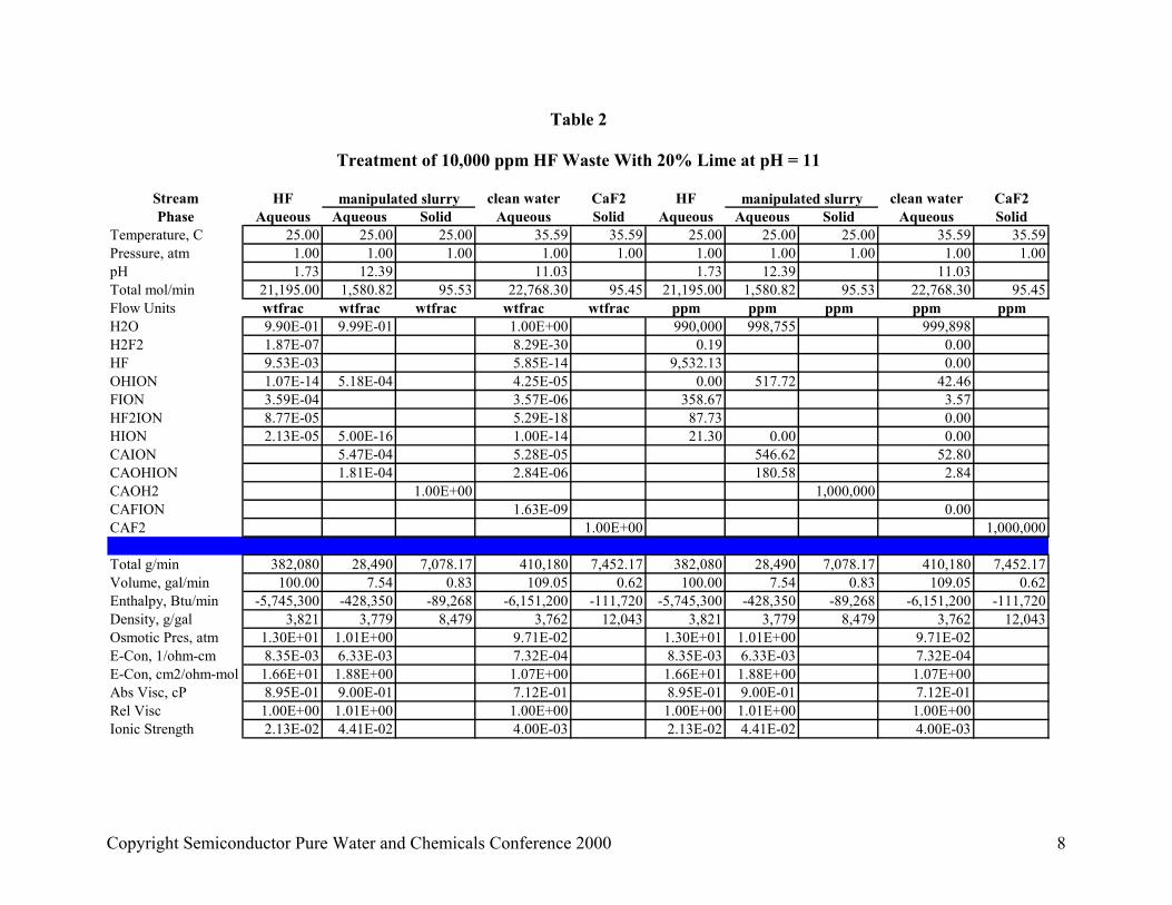
Treatment of a fluoride wastewater stream containing 10,000 ppm HF was also modeled, with

the same pH target of 11 using 20% lime. The results from model are given in Table 2. Since



Temperature, C 25.00 25.00 25.00 35.59 35.59 25.00 25.00 25.00 35.59 35.59Pressure, atm 1.00 1.00 1.00 1.00 1.00 1.00 1.00 1.00 1.00 1.00pH 1.73 12.39 11.03 1.73 12.39 11.03 Total mol/min 21,195.00 1,580.82 95.53 22,768.30 95.45 21,195.00 1,580.82 95.53 22,768.30 95.45Flow Units wtfrac wtfrac wtfrac wtfrac wtfrac ppm ppm ppm ppm ppmH2O 9.90E-01 9.99E-01 1.00E+00 990,000 998,755 999,898 H2F2 1.87E-07 8.29E-30 0.19 0.00 HF 9.53E-03 5.85E-14 9,532.13 0.00 OHION 1.07E-14 5.18E-04 4.25E-05 0.00 517.72 42.46 FION 3.59E-04 3.57E-06 358.67 3.57 HF2ION 8.77E-05 5.29E-18 87.73 0.00 HION 2.13E-05 5.00E-16 1.00E-14 21.30 0.00 0.00 CAION 5.47E-04 5.28E-05 546.62 52.80 CAOHION 1.81E-04 2.84E-06 180.58 2.84 CAOH2 1.00E+00 1,000,000 CAFION 1.63E-09 0.00 CAF2 1.00E+00 1,000,000

Total g/min 382,080 28,490 7,078.17 410,180 7,452.17 382,080 28,490 7,078.17 410,180 7,452.17Volume, gal/min 100.00 7.54 0.83 109.05 0.62 100.00 7.54 0.83 109.05 0.62Enthalpy, Btu/min -5,745,300 -428,350 -89,268 -6,151,200 -111,720 -5,745,300 -428,350 -89,268 -6,151,200 -111,720Density, g/gal 3,821 3,779 8,479 3,762 12,043 3,821 3,779 8,479 3,762 12,043Osmotic Pres, atm 1.30E+01 1.01E+00 9.71E-02 1.30E+01 1.01E+00 9.71E-02 E-Con, 1/ohm-cm 8.35E-03 6.33E-03 7.32E-04 8.35E-03 6.33E-03 7.32E-04 E-Con, cm2/ohm-mol 1.66E+01 1.88E+00 1.07E+00 1.66E+01 1.88E+00 1.07E+00 Abs Visc, cP 8.95E-01 9.00E-01 7.12E-01 8.95E-01 9.00E-01 7.12E-01 Rel Visc 1.00E+00 1.01E+00 1.00E+00 1.00E+00 1.01E+00 1.00E+00 Ionic Strength 2.13E-02 4.41E-02 4.00E-03 2.13E-02 4.41E-02 4.00E-03

manipulated slurry manipulated slurry


Table 2


more fluoride was present, the heat of reaction increased the temperature of the clean water to

35.59°C. The volume of clean water was 109.05 gpm, the result of adding 8.37 gpm of 20%

lime slurry to bring the pH of the clean water to 11.05.

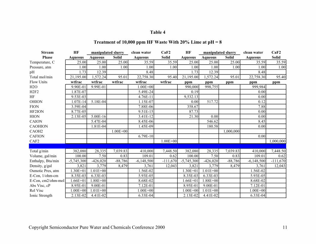
What if the target pH was 8 instead of 11? How does this affect temperature, volume, chemical

usage, and fluoride content? Treatment of both the 1,000 ppm and 10,000 ppm HF streams at pH

8 using the process of Figure 1 were modeled using ESP; the results are shown in Tables 3 and

4, respectively. Since the pH curve at 8 is quite steep, and it’s difficult to hit a specific target

with the high concentration of the 20% lime slurry, the pH tolerance had to be set at ±0.5 pH

units in order to get the calculations to converge.

At the lower pH, the fluoride ion content of the water rose to 7.3-7.9 ppm from the 3.5-4.0 ppm

values at the higher pH of 11. There was a very slight decrease in lime usage at the lower pH,

about 0.02 to 0.04 gpm less than at pH 11. This led to a slight decrease in the volume of the

clean water stream.

In a real-world application of process simulation software, a pilot system was operating on an HF

wastewater stream using lime as the chemical reactant. The pilot was easily achieving the target

discharge concentration of fluoride, below 20 ppm, when a sudden spike in the concentration of

fluoride in the clean water occurred. It was postulated that an increase in ammonia concentration

caused the problem, but samples were being analyzed off-site and results would not be returned

for days. In a matter of hours, ESP predicted that a high ammonia concentration in the

wastewater could have caused the fluoride spike. A solution to the problem was also modeled,

and shown to work by subsequent pilot operation. The analytical results confirmed the presence

of high levels of ammonia in the wastewater, at the same levels predicted by ESP to have caused

the problem. The process modeling shaved days off the process development time.

Laboratory Confirmation of Fluoride Waste Lime Treatment

The modeling results were compared to the results of laboratory experiments designed to

measure the soluble fluoride remaining after lime treatment of a synthetic fluoride waste. The



Temperature, C 25.00 25.00 25.00 26.11 26.11 25.00 25.00 25.00 26.11 26.11Pressure, atm 1.00 1.00 1.00 1.00 1.00 1.00 1.00 1.00 1.00 1.00pH 2.28 12.39 8.43 2.28 12.39 8.43 Total mol/min 20,971.70 155.48 9.40 21,125.00 9.37 20,971.70 155.48 9.40 21,125.00 9.37Flow Units wtfrac wtfrac wtfrac wtfrac wtfrac ppm ppm ppm ppm ppmH2O 9.99E-01 9.99E-01 1.00E+00 999,000 998,755 999,985 H2F2 1.53E-09 4.00E-24 0.00 0.00 HF 8.85E-04 4.49E-11 884.73 0.00 OHION 3.56E-14 5.18E-04 5.23E-08 0.00 517.72 0.05 FION 1.07E-04 7.27E-06 107.16 7.27 HF2ION 2.37E-06 8.12E-15 2.37 0.00 HION 5.75E-06 5.00E-16 3.82E-12 5.75 0.00 0.00 CAION 5.47E-04 7.73E-06 546.62 7.73 CAOHION 1.81E-04 5.24E-10 180.58 0.00 CAOH2 1.00E+00 1,000,000 CAFION 3.11E-10 0.00 CAF2 1.00E+00 1,000,000

Total g/min 377,820 2,802.17 696.17 380,580 731.53 377,820 2,802.17 696.17 380,580 731.53Volume, gal/min 100.00 0.74 0.08 100.89 0.06 100.00 0.74 0.08 100.89 0.06Enthalpy, Btu/min -5,681,600 -42,130 -8,780 -5,721,500 -10,973 -5,681,600 -42,130 -8,780 -5,721,500 -10,973Density, g/gal 3,778 3,779 8,479 3,772 12,043 3,778 3,779 8,479 3,772 12,043Osmotic Pres, atm 1.35E+00 1.01E+00 1.39E-02 1.35E+00 1.01E+00 1.39E-02 E-Con, 1/ohm-cm 2.25E-03 6.33E-03 4.45E-05 2.25E-03 6.33E-03 4.45E-05 E-Con, cm2/ohm-mol 4.52E+01 1.88E+00 6.24E-01 4.52E+01 1.88E+00 6.24E-01 Abs Visc, cP 8.92E-01 9.00E-01 8.69E-01 8.92E-01 9.00E-01 8.69E-01 Rel Visc 1.00E+00 1.01E+00 1.00E+00 1.00E+00 1.01E+00 1.00E+00 Ionic Strength 5.71E-03 4.41E-02 5.79E-04 5.71E-03 4.41E-02 5.79E-04



Table 3



Temperature, C 25.00 25.00 25.00 35.59 35.59 25.00 25.00 25.00 35.59 35.59Pressure, atm 1.00 1.00 1.00 1.00 1.00 1.00 1.00 1.00 1.00 1.00pH 1.73 12.39 8.48 1.73 12.39 8.48 Total mol/min 21,195.00 1,572.24 95.01 22,758.30 95.40 21,195.00 1,572.24 95.01 22,758.30 95.40Flow Units wtfrac wtfrac wtfrac wtfrac wtfrac ppm ppm ppm ppm ppmH2O 9.90E-01 9.99E-01 1.00E+00 990,000 998,755 999,984 H2F2 1.87E-07 5.49E-24 0.19 0.00 HF 9.53E-03 4.76E-11 9,532.13 0.00 OHION 1.07E-14 5.18E-04 1.15E-07 0.00 517.72 0.12 FION 3.59E-04 7.88E-06 358.67 7.88 HF2ION 8.77E-05 9.51E-15 87.73 0.00 HION 2.13E-05 5.00E-16 3.41E-12 21.30 0.00 0.00 CAION 5.47E-04 8.45E-06 546.62 8.45 CAOHION 1.81E-04 1.45E-09 180.58 0.00 CAOH2 1.00E+00 1,000,000 CAFION 6.79E-10 0.00 CAF2 1.00E+00 1,000,000

Total g/min 382,080 28,335 7,039.83 410,000 7,448.50 382,080 28,335 7,039.83 410,000 7,448.50Volume, gal/min 100.00 7.50 0.83 109.01 0.62 100.00 7.50 0.83 109.01 0.62Enthalpy, Btu/min -5,745,300 -426,020 -88,786 -6,148,500 -111,670 -5,745,300 -426,020 -88,786 -6,148,500 -111,670Density, g/gal 3,821 3,779 8,479 3,761 12,043 3,821 3,779 8,479 3,761 12,043Osmotic Pres, atm 1.30E+01 1.01E+00 1.56E-02 1.30E+01 1.01E+00 1.56E-02 E-Con, 1/ohm-cm 8.35E-03 6.33E-03 5.93E-05 8.35E-03 6.33E-03 5.93E-05 E-Con, cm2/ohm-mol 1.66E+01 1.88E+00 8.68E-02 1.66E+01 1.88E+00 8.68E-02 Abs Visc, cP 8.95E-01 9.00E-01 7.12E-01 8.95E-01 9.00E-01 7.12E-01 Rel Visc 1.00E+00 1.01E+00 1.00E+00 1.00E+00 1.01E+00 1.00E+00 Ionic Strength 2.13E-02 4.41E-02 6.33E-04 2.13E-02 4.41E-02 6.33E-04



Table 4


laboratory feed waste, containing either 1,000 ppm or 10,000 ppm HF, was synthesized with DI

water as the base stock. Using a typical jar testing apparatus, a 1 L beaker of the waste was

agitated with a paddle stirrer at a constant rate while solid lime was carefully added in small

portions to achieve the target pH. The results of the laboratory tests are shown in Table 5.

Unfiltered samples were taken of the supernatant after allowing the solids to settle. Soluble

fluoride was measured using a fluoride ion specific electrode (ISE) after adding a TSAB buffer

to the sample.

As shown in Table 5, the feed for experiment 1 contained 1,000 ppm HF. The pH was raised to

11.00 with lime, then samples were periodically taken of the supernatant. Note that the soluble

fluoride content of the water dropped to 10 ppm after 5 min. The pH drifted downward to 8.35,

reflecting consumption of lime by HF. Based on the result of experiment 2, the pH probably

dropped to 8.35 after only 5 min, but it was not measured for 60 min.

Samples were taken and treated with various portions of coagulants and/or flocculants, as

indicated in the last steps of experiment 1. KSP 340 is a proprietary coagulant sold by Koch

Microelectronic Service Co. (KMSC), while KSP 107 is a flocculant. It is interesting to note

that the soluble fluoride was reduced to 8.5 ppm from 9.5 ppm after treatment with the

coagulant/flocculant combination. While ESP can model the chemistry and solubility of the

system, the unit processes used are not capable of modeling the physical processes of

precipitation, coagulation, or flocculation10 (although such capability is being developed by

OLI). Some real-world experimentation or experience is necessary to complete the connection

between process simulation and the actual process.

Experiment 2 in Table 5 is an example of the real world variation from process simulation. The

lowest fluoride concentration achievable was 26 ppm. While the true source of the error isn’t

known, it can be conjectured that rapid precipitation of CaF2 coated the lime particles, making

the lime unavailable for reaction with the low concentration of HF remaining in solution.

Experiments 3 and 4 are additional examples of the requirement for use of coagulants and

flocculants to reduce soluble fluoride to levels below 20 ppm. Although the lab results don’t


Fluoride Removal from Synthetic HF Waste Using Lime in the Lab

HF conc. Wt. Lime [F-]Exp. ppm added, g pH ppm Comments

1 1,000 2.05 11.00 added lime to pH 11.010 after 5 min. stirring10 after 30 min. stirring

8.35 9.5 after 60 min. stirring8.6 after adding 10 ppm KSP 340 and 20 ppm KSP 107; very hazy8.5 after adding additional 10 ppm KSP 340 and 20 ppm KSP 107; light haze; fast settling floc8.1 fresh sample with 10 ppm KSP 340 and 20 ppm KSP 107; cloudy

2 10,000 21.71 11.00 added lime to pH 11.08.32 39 after 5 min. stirring

25 after 30 min. stirring32 after 60 min. stirring26 after adding 20 ppm KSP 340 and 300 ppm KSP 107; some floc, very cloudy supernatent29 fresh sample with 10 ppm KSP 340 and 200 ppm KSP 107; some floc with very cloudy supernatent

3 1,000 1.99 7.20 initial pH after lime = 9.0; added H2SO4 to 7.226 after 5 min. stirring26 after 30 min. stirring

8.45 25 after 60 min. stirring16 after adding 10 ppm KSP 340 and 10 ppm KSP 107; hazy, not clear, some floc14 after adding additional 20 ppm KSP 107; light haze; fast settling time15 fresh sample with 10 ppm KSP 340 and 20 ppm KSP 107; cloudy13 fresh sample with 10 ppm KSP 340 and 30 ppm KSP 107; near clear plus floc

4 10,000 18.99 8.10 added lime to pH 838 after 5 min. stirring44 after 30 min. stirring

7.93 41 after 60 min. stirring14 after adding 160 ppm KSP 107; very clear plus floc14 fresh sample with 10 ppm KSP 340 and 160 ppm KSP 107; slightly less clear than previous sample

Table 5


exactly match the modeling results, modeling predicted the doubling of the fluoride

concentration on lowering the pH from 11 to 8. The experiments confirmed that increase.

There is good agreement between prediction and experiment as far as the amount of lime

necessary to produce the intended results. The process simulations predicted that between 1.85

and 1.90 g of lime would be used per g of HF in the system. In the laboratory between 1.9 and

2.1 g of lime was used per g of HF.

Hydrofluoric Acid Wastewater Treatment with CaCl 2

HF wastewater from semiconductor fabs often contains unusual components. In order to

determine the usefulness of process simulation in such real-world situations, the calcium chloride

treatment of a complex wastewater containing 1,000 ppm HF, 1,000 ppm sulfuric acid, 300 ppm

acetic acid, 350 ppm NH4OH, and 400 ppm phosphoric acid was modeled. The pH of the stream

was arbitrarily set at 7.55 by adding 2,920 ppm of NaOH. Figure 2 is a PFD for the process

simulation used.

Figure 2

35% CaCl2

Synthetic HF Stream clean water

NaOH or H2SO4

CaF2 solids

Separator

fluoride meter

flow controller

pH meter

flow controller


When using CaCl2 two control loops are needed; one to control the CaCl2 addition rate, and one

to control the addition rate of the acid or base used to set the pH. The pH was set at either 3.5 or

8.0. Since the pH of the wastewater was 7.55, NaOH was added to raise the pH to 8.0, and

H2SO4 was used to lower the pH to 3.5. As in the lime process, the pH control loop was used to

achieve the desired pH target.

With ESP the concentration of components of the clean water can be monitored, and the

information can be used to control chemical addition rates in order to meet fluoride discharge

limits. In this case, the soluble fluoride content of the clean water was set at 7 ppm to give the

facility breathing room below the typical 15-20 ppm discharge limit. The second control loop

was used to set the CaCl2 addition rate to meet the 7 ppm fluoride target.

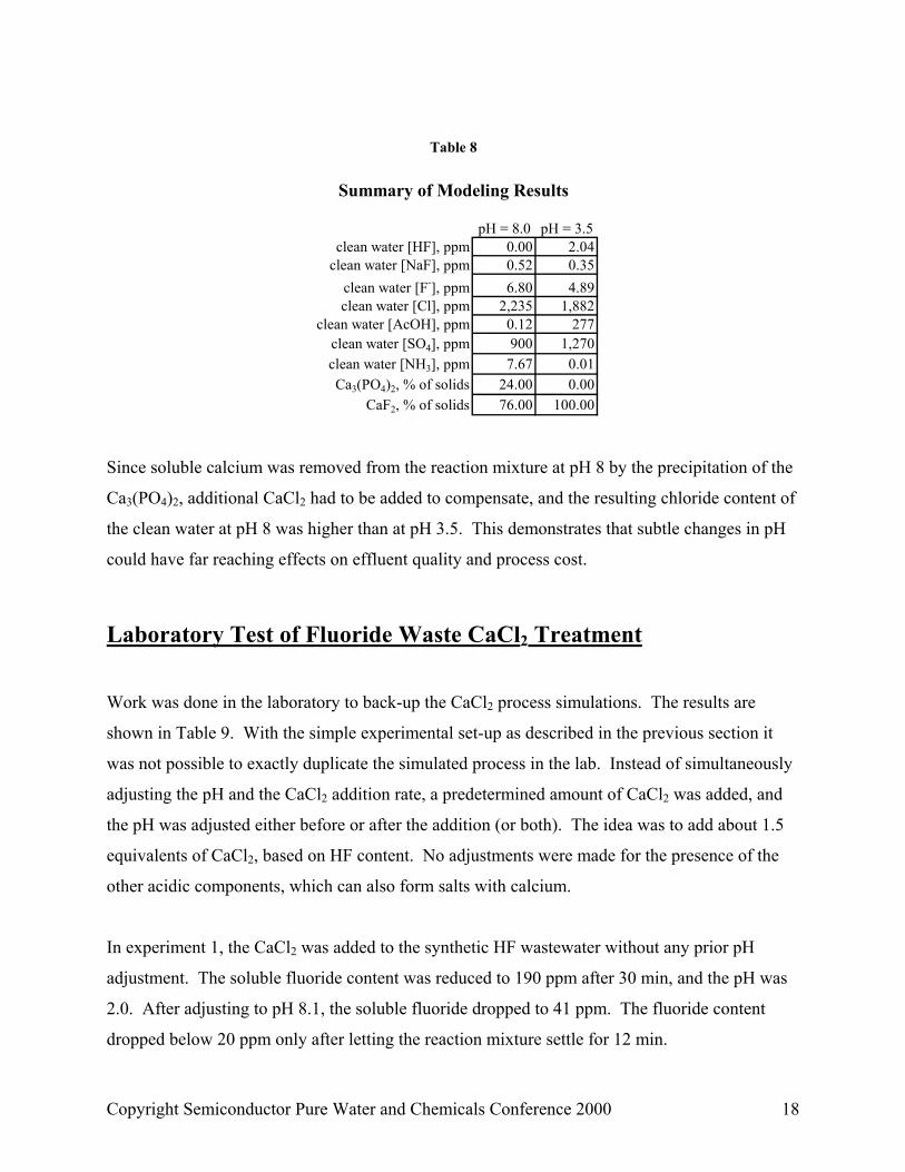
The results of the process simulations at pH 8 or 3.5 are shown in Tables 6 and 7 respectively,

with a summary in Table 8. At pH 8, the fluoride content of the clean water was about 7,

composed of 0.52 ppm of NaF and 6.80 ppm of fluoride ion. The chloride content was 2,235

ppm, the acetic acid content was 0.12 ppm, the sulfate content was 900 ppm and the ammonia

content was 7.67 ppm. The precipitated solid contained 24% Ca3(PO4)2 and 76% CaF2.

Contrast the results at pH 8 with the results at pH 3.5. The fluoride content was again about 7

ppm, composed of 2.04 ppm HF, 0.35 ppm NaF, and 4.89 ppm fluoride ion. The chloride

content was 1,882 ppm, the acetic acid content was 277 ppm, the sulfate content was 1,270 ppm,

and the ammonia content was less than 0.01 ppm. The differing results reflect the equilibrium

compositions at the two pH values.


Syn. HF Component ppmWater 994,030HF 1,000H2SO4 1,000H3PO4 400Acetic Acid 300NH4OH 350NaOH 2,920

Stream Synthetic HF CaCl2 NaOH clean waste precipitatePhase Aqueous Aqueous Aqueous Aqueous Solid

Temperature, C 25.00 25.00 25.00 25.18 25.18Pressure, atm 1.00 1.00 1.00 1.00 1.00pH 7.55 5.42 14.45 8.05 Total mol/min 26,240 217.58 52.42 26,470 12.70Flow Units ppm ppm ppm ppm ppmH2O 995,525 650,000 900,000 994,499 ACETACID 0.38 0.12HF 0.03 0.00NH3 2.47 7.67NAACET 12.90 13.86NAF 65.35 0.52NH4ACET 3.33 3.16OHION 0.01 0.00 42,521.30 0.03 FION 920.00 6.80H2PO4ION 66.03 0.23HP2O7ION 0.02 0.00HPO4ION 326.38 3.61NA2FION 0.06 0.00NAION 1,633.51 57,478.80 1,767.32NASO4ION 28.18 29.64NH4ION 169.75 163.11NH4SO4ION 44.27 41.00ACETATEION 282.76 278.86PO4ION 0.02 0.00SO4ION 919.43 900.40CAION 126,390 32.44CAOHION 0.02 0.00CLION 223,609 2,234.66CAACET2 0.09CASO4 16.10CAACETION 1.24CAPO4ION 0.14CA3PO42 244,463CAF2 755,537

Total g/min 473,550 4,777.67 953.88 478,070 1,213.85Volume, gal/min 125.00 0.94 0.23 126.21 0.10Enthalpy, Btu/min -7.11E+06 -5.91E+04 -1.40E+04 -7.17E+06 -1.75E+04Density, g/gal 3,788.44 5,059.58 4,143.51 3,788.06 12,039.50Osmotic Pres, atm 3.16 932.43 169.76 3.54 E-Con, 1/ohm-cm 7.20E-03 1.73E-01 3.09E-01 9.19E-03 E-Con, cm2/ohm-mol 4.72E+01 4.10E+01 1.13E+02 9.81E+01 Abs Visc, cP 9.08E-01 4.86E+00 1.59E+00 8.97E-01 Rel Visc 1.02E+00 5.45E+00 1.78E+00 1.01E+00 Ionic Strength 9.39E-02 1.46E+01 2.78E+00 9.83E-02

Treatment Of HF Wastewater with CaCl2 at pH 8

Table 6


Syn. HF Component ppmWater 994,030HF 1,000H2SO4 1,000H3PO4 400Acetic Acid 300NH4OH 350NaOH 2,920

Stream Synthetic HF CaCl2 H2SO4 clean waste precipitatePhase Aqueous Aqueous Aqueous Aqueous Solid

Temperature, C 25.00 25.00 25.00 25.18 25.18Pressure, atm 1.00 1.00 1.00 1.00 1.00pH 7.55 5.42 -0.03 3.49 Total mol/min 26,240 183.55 109.39 26,495 11.75Flow Units ppm ppm ppm ppm ppmH2O 995,525 650,000 900,000 994,105 ACETACID 0.38 277.41HF 0.03 2.04NH3 2.47 0.00NAACET 12.90 0.84NAF 65.35 0.35NH4ACET 3.33 0.21H3PO4 0.00 12.73OHION 0.01 0.00 0.00 0.00 FION 920.00 4.89H2P2O7ION 0.00 0.02H2PO4ION 66.03 370.69HION 0.00 0.00 1,188.25 0.42 HP2O7ION 0.02 0.00HPO4ION 326.38 0.16HSO4ION 0.00 83,511.80 16.54NA2FION 0.06 0.00NAION 1,633.51 1,652.23NASO4ION 28.18 38.65NH4ION 169.75 168.77NH4SO4ION 44.27 59.28ACETATEION 282.76 18.14PO4ION 0.02 0.00SO4ION 919.43 15,299.90 1,269.52CAION 126,390 64.34CAOHION 0.02 0.00CLION 223,610 1,882.42CASO4 43.77CAACETION 0.16CAH2PO4ION 11.46CAF2 1,000,000

Total g/min 473,550 4,030.33 2,097.33 478,770 917.15Volume, gal/min 125.00 0.80 0.52 126.33 0.08Enthalpy, Btu/min -7.11E+06 -4.99E+04 -3.02E+04 -7.18E+06 -1.38E+04Density, g/gal 3,788.44 5,059.58 4,031.08 3,789.95 12,043.30Osmotic Pres, atm 3.16E+00 9.32E+02 6.04E+01 3.35E+00 E-Con, 1/ohm-cm 7.20E-03 1.73E-01 4.37E-01 8.91E-03 E-Con, cm2/ohm-mol 4.72E+01 4.10E+01 4.03E+02 1.01E+02 Abs Visc, cP 9.08E-01 4.86E+00 1.13E+00 8.98E-01 Rel Visc 1.02E+00 5.45E+00 1.27E+00 1.01E+00 Ionic Strength 9.39E-02 1.46E+01 1.49E+00 1.00E-01

Treatment Of HF Wastewater with CaCl2 at pH 3.5

Table 7


pH = 8.0 pH = 3.5clean water [HF], ppm 0.00 2.04

clean water [NaF], ppm 0.52 0.35clean water [F-], ppm 6.80 4.89clean water [Cl], ppm 2,235 1,882

clean water [AcOH], ppm 0.12 277clean water [SO4], ppm 900 1,270clean water [NH3], ppm 7.67 0.01Ca3(PO4)2, % of solids 24.00 0.00

CaF2, % of solids 76.00 100.00

Summary of Modeling Results

Table 8

Since soluble calcium was removed from the reaction mixture at pH 8 by the precipitation of the

Ca3(PO4)2, additional CaCl2 had to be added to compensate, and the resulting chloride content of

the clean water at pH 8 was higher than at pH 3.5. This demonstrates that subtle changes in pH

could have far reaching effects on effluent quality and process cost.

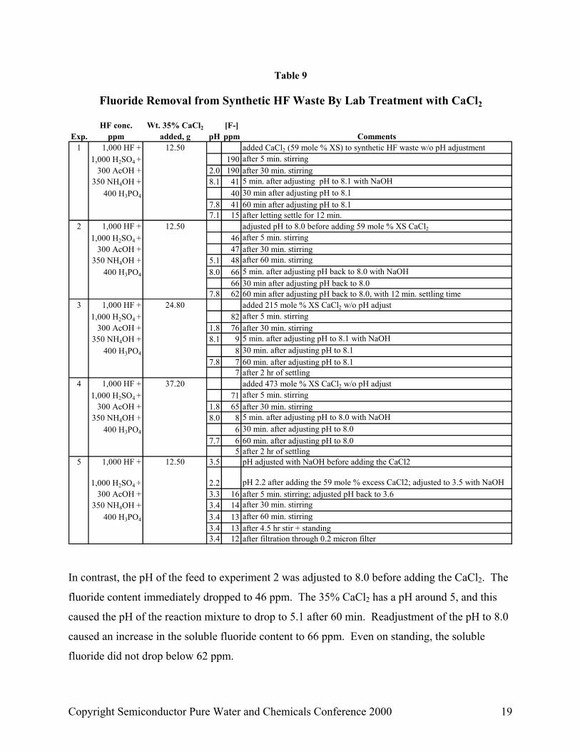
Laboratory Test of Fluoride Waste CaCl 2 Treatment

Work was done in the laboratory to back-up the CaCl2 process simulations. The results are

shown in Table 9. With the simple experimental set-up as described in the previous section it

was not possible to exactly duplicate the simulated process in the lab. Instead of simultaneously

adjusting the pH and the CaCl2 addition rate, a predetermined amount of CaCl2 was added, and

the pH was adjusted either before or after the addition (or both). The idea was to add about 1.5

equivalents of CaCl2, based on HF content. No adjustments were made for the presence of the

other acidic components, which can also form salts with calcium.

In experiment 1, the CaCl2 was added to the synthetic HF wastewater without any prior pH

adjustment. The soluble fluoride content was reduced to 190 ppm after 30 min, and the pH was

2.0. After adjusting to pH 8.1, the soluble fluoride dropped to 41 ppm. The fluoride content

dropped below 20 ppm only after letting the reaction mixture settle for 12 min.


Fluoride Removal from Synthetic HF Waste By Lab Treatment with CaCl2

HF conc. Wt. 35% CaCl2 [F-]Exp. ppm added, g pH ppm Comments

1 1,000 HF + 12.50 added CaCl2 (59 mole % XS) to synthetic HF waste w/o pH adjustment1,000 H2SO4 + 190 after 5 min. stirring

300 AcOH + 2.0 190 after 30 min. stirring350 NH4OH + 8.1 41 5 min. after adjusting pH to 8.1 with NaOH

400 H3PO4 40 30 min after adjusting pH to 8.17.8 41 60 min after adjusting pH to 8.17.1 15 after letting settle for 12 min.

2 1,000 HF + 12.50 adjusted pH to 8.0 before adding 59 mole % XS CaCl21,000 H2SO4 + 46 after 5 min. stirring

300 AcOH + 47 after 30 min. stirring350 NH4OH + 5.1 48 after 60 min. stirring

400 H3PO4 8.0 66 5 min. after adjusting pH back to 8.0 with NaOH66 30 min after adjusting pH back to 8.0

7.8 62 60 min after adjusting pH back to 8.0, with 12 min. settling time3 1,000 HF + 24.80 added 215 mole % XS CaCl2 w/o pH adjust

1,000 H2SO4 + 82 after 5 min. stirring300 AcOH + 1.8 76 after 30 min. stirring

350 NH4OH + 8.1 9 5 min. after adjusting pH to 8.1 with NaOH400 H3PO4 8 30 min. after adjusting pH to 8.1

7.8 7 60 min. after adjusting pH to 8.17 after 2 hr of settling

4 1,000 HF + 37.20 added 473 mole % XS CaCl2 w/o pH adjust1,000 H2SO4 + 71 after 5 min. stirring

300 AcOH + 1.8 65 after 30 min. stirring350 NH4OH + 8.0 8 5 min. after adjusting pH to 8.0 with NaOH

400 H3PO4 6 30 min. after adjusting pH to 8.07.7 6 60 min. after adjusting pH to 8.0

5 after 2 hr of settling5 1,000 HF + 12.50 3.5 pH adjusted with NaOH before adding the CaCl2

1,000 H2SO4 + 2.2 pH 2.2 after adding the 59 mole % excess CaCl2; adjusted to 3.5 with NaOH300 AcOH + 3.3 16 after 5 min. stirring; adjusted pH back to 3.6

350 NH4OH + 3.4 14 after 30 min. stirring400 H3PO4 3.4 13 after 60 min. stirring

3.4 13 after 4.5 hr stir + standing3.4 12 after filtration through 0.2 micron filter

Table 9

In contrast, the pH of the feed to experiment 2 was adjusted to 8.0 before adding the CaCl2. The

fluoride content immediately dropped to 46 ppm. The 35% CaCl2 has a pH around 5, and this

caused the pH of the reaction mixture to drop to 5.1 after 60 min. Readjustment of the pH to 8.0

caused an increase in the soluble fluoride content to 66 ppm. Even on standing, the soluble

fluoride did not drop below 62 ppm.


In experiments 3 and 4 a large excess of CaCl2 was added without prior pH adjustment of the

feed. In both cases, soluble fluoride concentrations below 10 ppm were not achieved until the

pH of the reaction mixture was raised to 8.0.

In experiment 5, the pH of the feed was adjusted to 3.5 using NaOH. The pH was readjusted to

3.5 after adding the excess CaCl2. The soluble fluoride content was 16 ppm, dropping to 13 ppm

after stirring for 60 min. This is a better result than that obtained under the same conditions at

pH 8 of experiment 1, which required settling before achieving the low soluble fluoride content.

At pH 3.5, ESP predicted that 1.08 equivalents, or 8 mole % excess, CaCl2 would be needed to

produce a soluble fluoride content of 7 ppm. In the lab 1.59 eq. CaCl2, or 59 mole % excess,

only reduced the soluble fluoride content to 13 ppm. At pH 8, ESP predicted that 1.28 eq.

CaCl2, 28 mole % excess, would be required to achieve the target soluble fluoride concentration

of 7 ppm while the lab work indicated that a much larger excess of 3.15 eq., or 215 mole %

excess, was necessary. Recall that the ESP calculations were based on strict thermodynamics,

with no kinetic factors taken into consideration. The difference between prediction and lab can

then be attributed to the simulation being in thermodynamic equilibrium. Given enough time,

the lab results probably would have closely resembled the simulation results. The conclusion is

that retention time, and issues associated with retention time, will be a very important factor in

designing a full-size system. It is possible to factor kinetics into a process simulation, but that is

beyond the intentions of this paper. Piloting the treatment of the wastewater would be the most

valuable exercise.

Neutralization of Dilute Acid Wastewater

Most of the time, the analysis of a wastewater stream only indicates the concentrations of anions

and cations, and a few other parameters. How are these components put together, i.e. is “sulfate”

present as sodium sulfate or sulfuric acid? If the pH is changed or a treatment chemical is added,

what compositional changes occur?


Stream Dilute Acid neutral water Dilute Acid neutral waterPhase Aqueous Aqueous Solid Aqueous Aqueous Aqueous Solid Aqueous

Temperature, C 25.00 25.00 25.00 25.01 25.00 25.00 25.00 25.01Pressure, atm 1.00 1.00 1.00 1.00 1.00 1.00 1.00 1.00pH 3.17 12.39 7.94 3.17 12.39 7.94Total mol/min 20,946.70 11.06 0.14 20,958.30 20,946.70 11.06 0.14 20,958.30Flow Units wtfrac wtfrac wtfrac wtfrac ppm ppm ppm ppmH2O 1.00E+00 9.99E-01 1.00E+00 999,944 998,755 999,929H2F2 3.19E-16 3.77E-25 0.00 0.00H2SO4 1.77E-20 5.03E-30 0.00 0.00HCL 1.10E-14 1.84E-19 0.00 0.00HF 4.05E-07 1.39E-11 0.40 0.00HNO3 1.87E-10 3.13E-15 0.00 0.00NH3 5.47E-12 3.08E-07 0.00 0.31SO3 1.87E-24 0.00KHSO4 1.20E-13 2.01E-18 0.00 0.00NAF 1.62E-11 3.29E-11 0.00 0.00NANO3 3.74E-12 3.69E-12 0.00 0.00CASO4 1.91E-08 5.96E-07 0.02 0.60NH4NO3 1.49E-08 1.40E-08 0.01 0.01KCL 3.10E-12 3.06E-12 0.00 0.00OHION 2.66E-13 5.18E-04 1.59E-08 0.00 517.72 0.02CAION 4.81E-07 5.47E-04 1.53E-05 0.48 546.62 15.31CANO3ION 2.52E-10 7.84E-09 0.00 0.01CAOHION 1.55E-16 1.81E-04 2.89E-10 0.00 180.58 0.00CLION 2.78E-05 2.78E-05 27.80 27.78FION 3.66E-07 7.50E-07 0.37 0.75HF2ION 3.69E-12 2.60E-16 0.00 0.00HION 7.08E-07 5.00E-16 1.20E-11 0.71 0.00 0.00HSO4ION 6.94E-07 1.18E-11 0.69 0.00KION 2.71E-07 2.71E-07 0.27 0.27KSO4ION 7.58E-10 7.58E-10 0.00 0.00NA2FION 7.63E-18 1.55E-17 0.00 0.00NAION 6.46E-07 6.45E-07 0.65 0.65NASO4ION 3.75E-10 3.75E-10 0.00 0.00NH4ION 7.10E-06 6.77E-06 7.10 6.77NH4SO4ION 6.13E-08 5.85E-08 0.06 0.06NO3ION 5.71E-06 5.70E-06 5.71 5.70CAFION 8.60E-13 5.50E-11 0.00 0.00SO4ION 1.21E-05 1.24E-05 12.11 12.39CAOH2 1.00E+00 1,000,000

Total g/min 377,370 199.24 10.23 377,570 377,370 199.24 10.23 377,570Volume, gal/min 100.00 0.05 0.00 100.05 100.00 0.05 0.00 100.05Enthalpy, Btu/min -5.67E+06 -3.00E+03 -1.29E+02 -5.68E+06 -5.67E+06 -3.00E+03 -1.29E+02 -5.68E+06Density, g/gal 3,773.60 3,778.97 8,478.56 3,773.68 3,773.60 3,778.97 8,478.56 3,773.68Osmotic Pres, atm 0.05 1.01 0.04 0.05 1.01 0.04E-Con, 1/ohm-cm 3.57E-04 6.33E-03 1.55E-04 3.57E-04 6.33E-03 1.55E-04E-Con, cm2/ohm-mol 2.59E+02 8.94E+00 8.72E+01 2.59E+02 8.94E+00 8.72E+01Abs Visc, cP 8.91E-01 9.00E-01 8.91E-01 8.91E-01 9.00E-01 8.91E-01Rel Visc 1.00E+00 1.01E+00 1.00E+00 1.00E+00 1.01E+00 1.00E+00Ionic Strength 1.29E-03 4.41E-02 1.69E-03 1.29E-03 4.41E-02 1.69E-03


Neutralization of Dilute Acid With Lime

Table 10


As an example, an analysis of a dilute acid wastewater showed 100 ppm sulfate, 50 ppm

chloride, 5 ppm fluoride, 20 ppm nitrate, 10 ppm sodium, 20 ppm ammonium, 5 ppm potassium,

and 2 ppm calcium. The measured pH was 3.17. Given these ionic components, what molecular

species were actually present in the water, and what happened when the water was neutralized to

pH 8 using dilute lime?

An application called WaterAnalyzer in the OLI suite of programs was used to charge balance

the analysis, and to output a stream containing the molecular species corresponding to the anions

and cations present in the water. This stream was then used to feed a neutralization process in

ESP, where the flow of 5% lime was controlled using a pH controller in order to achieve 8 pH.

The data is presented in Table 10.

Note that the Dilute Acid feedstock contained 33 components including water. Some of these

components were neutral species such as H2F2, H2SO4, and HCl, and some were ionic species

such as hydroxide anion and hydrogen cation. As expected in a pH change, neutralization

produced exponential changes in the concentrations of six components, as summarized in Table

11.

dilute acid neutral water[HF], ppm 0.40 0.000014

[NH3], ppm 0.0000055 0.31[CaSO4], ppm 0.02 0.60

[Ca++], ppm 0.48 15.31[H+], ppm 0.71 0.000012

[HSO4-], ppm 0.69 0.000012

Neutralization of Dilute Acid

Table 11

While the simulation results are not earth shattering, they illustrate the huge changes in

composition which can occur on carrying out simple pH changes. The simulation becomes more

valuable as the complexity of the system increases. For instance, if the ammonium concentration

of the wastewater was hundreds of ppm, the neutral water could evolve gaseous ammonia at


levels above safe exposure limits, necessitating a closed system. With process simulation, one

could examine myriad pH and concentration scenarios before designing the final system.

Wastewater from CMP Operations

Chemical mechanical planarization (CMP) is a new technology for producing smooth surfaces

on semiconductor chips. An aqueous slurry of silica or alumina is used along with a rotating

CMP pad to “wet sand” metal or oxide surfaces. The wastewater from CMP operations can

contain high concentrations of solids, typically 1,000 ppm, and other components removed from

the chip. Clarification or filtration is used to remove the solids if the POTW has limitations on

solids discharge. In order to design an acceptable process, the solubility of the silica, alumina,

and other components under different conditions of pH, temperature, etc., should be known. In

this section the water solubility of alumina and silica at various pH values will be determined

(process simulation of clarification or filtration will be the subject of a future publication). This

information can be used to adjust the pH of the wastewater to its optimal value for removal of the

solids.

The chemistry of silica is quite complex11 and cannot begin to be addressed by this paper. The

chemistry of alumina is simpler but still formidable12. The combination of the two can produce

alumino-silicates of indeterminate structure. Process simulation can be used to point out

potential operating ranges; each situation would have to be optimized based on its particular

components and conditions.

A simple wastewater containing only 1,000 ppm of SiO2 and 1,000 ppm of Al(OH)3 was titrated

between pH 2 and pH 12 using either NaOH or H2SO4 as titrants. Equilibrium calculations in

OLI’s Express Calculate application determined that the natural pH of the mixture was 6.05.

The pH of the system was varied in 0.2 pH increments, using H2SO4 to lower the pH below the

natural pH, and NaOH to raise the pH above the natural pH. At each pH value, the equilibrium

composition of the mixture was determined. The data is presented in Chart 1.


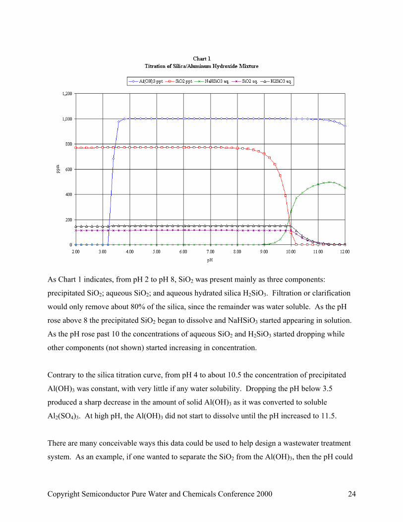
As Chart 1 indicates, from pH 2 to pH 8, SiO2 was present mainly as three components:

precipitated SiO2; aqueous SiO2; and aqueous hydrated silica H2SiO3. Filtration or clarification

would only remove about 80% of the silica, since the remainder was water soluble. As the pH

rose above 8 the precipitated SiO2 began to dissolve and NaHSiO3 started appearing in solution.

As the pH rose past 10 the concentrations of aqueous SiO2 and H2SiO3 started dropping while

other components (not shown) started increasing in concentration.

Contrary to the silica titration curve, from pH 4 to about 10.5 the concentration of precipitated

Al(OH)3 was constant, with very little if any water solubility. Dropping the pH below 3.5

produced a sharp decrease in the amount of solid Al(OH)3 as it was converted to soluble

Al2(SO4)3. At high pH, the Al(OH)3 did not start to dissolve until the pH increased to 11.5.

There are many conceivable ways this data could be used to help design a wastewater treatment

system. As an example, if one wanted to separate the SiO2 from the Al(OH)3, then the pH could


be set at 2.5, and the solid silica could be removed from the dissolve Al(OH)3. Or conversely,

the pH could be set at 10.25 and the solid Al(OH)3 could be filtered away from the dissolved

silica.

Treatment of Cu CMP Wastewater

Wastewater from copper CMP tools contains from 5 to 100 ppm soluble copper, usually in the

form of Cu+2 (cupric ion). The slurries used can be either silica or alumina based. Depending on

the slurry manufacturer, other components such as oxidizers or chelants can be present. A

typical component in slurries is ammonia, which can form copper chelation compounds.

The discharge limitations for copper vary by location, but are generally <1.50 ppm. One method

of treating copper-containing wastewater is to raise the pH to form cupric hydroxide (Cu(OH)2),

which precipitates from solution, and can be removed along with other solids present in the

system by clarification or filtration. What is the optimal pH range for precipitation of Cu(OH)2?

Express Calculate was used to complete a pH survey. A wastewater feed containing 154 ppm

Cu(OH)2 (equivalent to 100 ppm Cu+2) was titrated with either NaOH or H2SO4. Below the

natural pH of 6.05, H2SO4 was used to lower the pH. Above 6.05 pH, NaOH was used to raise

the pH. The data is presented in Chart 2.

Below about pH 4.5 all of the Cu+2 was in solution. As the system approached pH 6, the Cu+2

started precipitating as Cu(OH)2. At pH 8 all of the copper had precipitated from solution. The

optimal pH for removing copper from the wastewater via clarification or filtration was therefore

at or above 8.

When 1,000 ppm ammonia was added to the system, the situation changed drastically, as shown

in Chart 3. Ammonia will form cupric ion complexes above pH 6. These complexes have the

molecular formulas Cu(NH3)2+2, Cu(NH3)3

+2, Cu(NH3)4+2, and Cu(NH3)5

+2. The concentrations

of each complex depend on the relative concentrations of copper and ammonia and the pH. The

higher the concentration of ammonia and the higher the pH, the more of the tetra- and


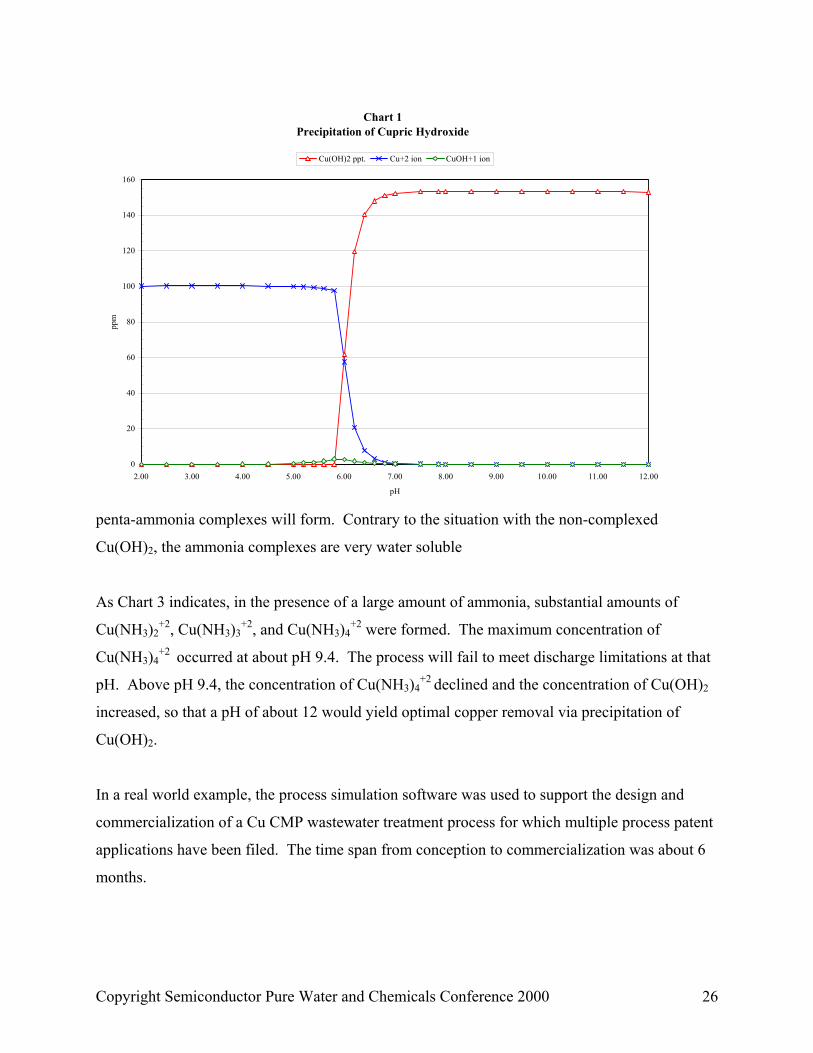
Chart 1Precipitation of Cupric Hydroxide

0

20

40

60

80

100

120

140

160

2.00 3.00 4.00 5.00 6.00 7.00 8.00 9.00 10.00 11.00 12.00

pH

ppm

Cu(OH)2 ppt. Cu+2 ion CuOH+1 ion

penta-ammonia complexes will form. Contrary to the situation with the non-complexed

Cu(OH)2, the ammonia complexes are very water soluble

As Chart 3 indicates, in the presence of a large amount of ammonia, substantial amounts of

Cu(NH3)2+2, Cu(NH3)3

+2, and Cu(NH3)4+2 were formed. The maximum concentration of

Cu(NH3)4+2 occurred at about pH 9.4. The process will fail to meet discharge limitations at that

pH. Above pH 9.4, the concentration of Cu(NH3)4+2 declined and the concentration of Cu(OH)2

increased, so that a pH of about 12 would yield optimal copper removal via precipitation of

Cu(OH)2.

In a real world example, the process simulation software was used to support the design and

commercialization of a Cu CMP wastewater treatment process for which multiple process patent

applications have been filed. The time span from conception to commercialization was about 6

months.


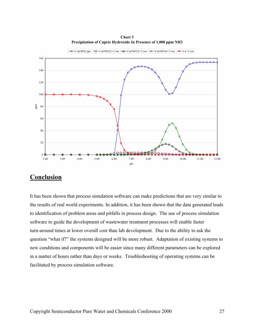
Chart 3Precipitation of Cupric Hydroxide In Presence of 1,000 ppm NH3

0

20

40

60

80

100

120

140

160

2.00 3.00 4.00 5.00 6.00 7.00 8.00 9.00 10.00 11.00 12.00

pH

ppm

Cu(OH)2 ppt. Cu(NH3)2+2 ion Cu(NH3)3+2 ion Cu(NH3)4+2 ion Cu+2 ion

Conclusion

It has been shown that process simulation software can make predictions that are very similar to

the results of real world experiments. In addition, it has been shown that the data generated leads

to identification of problem areas and pitfalls in process design. The use of process simulation

software to guide the development of wastewater treatment processes will enable faster

turn-around times at lower overall cost than lab development. Due to the ability to ask the

question “what if?” the systems designed will be more robust. Adaptation of existing systems to

new conditions and components will be easier since many different parameters can be explored

in a matter of hours rather than days or weeks. Troubleshooting of operating systems can be

facilitated by process simulation software.


Acknowledgement The authors thank Dick Hansen, of Koch Industries’ Analytical Services Department in Wichita,

Kansas, for carrying out the lime and CaCl2 HF treatment experiments. DKJ thanks David

Tolson, President of KMSC, for enthusiastic encouragement to seek out information concerning

process simulation software.

Biography Dustin K. James has been working as Chemistry and Technology Manager in the Water Reclaim

Group of KMSC for 17 months. Prior he was employed with Koch Specialty Chemical Co., first

as a Principal Research Chemist in process and product development at the R&D lab in Wichita,

Kansas, for 9 ½ years, then as the Technology Exploitation Manager in Houston, Texas, for 1

year. Dustin is a co-inventor on three granted process patents, and three additional patent

applications. He received his Bachelor of Science degree in Chemistry from Southwestern

University in Georgetown, Texas, and his Ph.D. in organic synthetic chemistry from The

University of Texas at Austin. Prior to working for Koch Industries, Inc., Dustin was employed

by Norwich Eaton Pharmaceuticals (a subsidiary of Procter and Gamble) in Norwich, New York,

as a Staff Scientist in the Process Development lab. He is a member of the American Chemical

Society and TAPPI.

Anthony J. Gerbino is a Principal at Aqueous Process Simulations. Prior to that, AJ worked at

OLI Systems as a Technical Scientist for 5 years. AJ obtained his Bachelor of Science in

Chemistry from The University of Texas at Austin and his Ph.D. in Aqueous Chemistry from

Rice University. He has authored numerous papers on scaling, oil and gas production, and

aqueous chemistry.



References 1 International Technology Roadmap for Semiconductors 1998 Update, Sponsored by the

Semiconductor Industry Association 2 AspenTech’s products include Aspen Plus and BATCHFRAC for doing process design,

among a list of 20 or more software packages for design, control, and optimization. More

information can be obtained from their web page at http://www.aspentech.com/index.htm. 3 Simulation Science, Inc.’s products include the Process Engineering Suite of PRO/II,

HEXTRAN, DATACON, INPLANT, and VISUAL FLOW. More information can be obtained

from their web page at http://www.simsci.com/index_old.htm. 4 See Pacific Simulations, Inc.’s web page at http://www.pacsim.com/default.shtml. 5 J.M. Spooner “Review of Computer Process Simulation in Industrial Pollution Prevention”

Report (1994), EPA/600/R-94/128; Order No. PB95-154886, 56 pp. Avail.: HTIS 6 Details and contact information can be found at OLI Systems’ web page

http://www.olisystems.com/. 7 Information about French Creek Software’s programs can be found on their web page at

http://www.frenchcreeksoftware.com/. 8 The OLI engine framework is based upon:

• “the revised Helgeson equation of state for predicting the partial molar standard-state

thermodynamic properties of all species, including organics, in water;”

• “the Bromley-Zematis framework for the prediction of excess thermodynamic properties of

ions;”

• “the Pitzer and Setschenow formulation for the prediction of excess thermodynamic

properties calculation of molecular species in water; and”

• “the Enhanced SRK equation of state for the prediction of vapor and non-aqueous, liquid

phase themodynamic properties. This enhanced equation of state applies to organics which

are sparingly soluble in water, and which form a second liquid phase which is largely ideal.”

Jim Berthold “A Guide to Using ESP” OLI Systems, Inc., 1999, Chapter 1, page 3.


9 Punnchalee Laothumthut, Chemistry and Chemical Process Studies of Fluoride Removal in a

Silicon Wafer Manufacturing Wastewater Treatment Plant, M.S.Thesis, Oregon State University,

20 March 1996. 10 Yong H. Kim, Ph.D., Coagulants and Flocculants: Theory and Practice, Tall Oaks Publishing,

Littleton, CO, 1995. 11 Ralph K. Iler; The Chemistry of Silica: Solubility, Polymerization, Colloid, and Surface

Properties, and Biochemistry, John Wiley and Sons, New York, 1979. 12 Garrison Sposito, Ph.D., Editor, The Environmental Chemistry of Aluminum 2nd Edition, Lewis

Publishers, Boca Raton, Florida, 1996.

using process simulation to predict wastewater treatment …dustin/spwccpaper3.pdf · lastly, it...

Documents