Using Product Text to Capture Vertical Integrationand Firm Boundaries

Laurent Fresard, Gerard Hoberg and Gordon Phillips∗

August 28, 2017

ABSTRACT

We construct new dynamic measures of vertical integration and relatedness bylinking product text from the BEA input-output tables to product text in firm 10-Ks. We use these text-based measures to examine changes in vertical integrationand firm boundaries created by acquisitions and organic changes in production. Wefind that the stage of innovation is important. Firms in R&D intensive industriesare less likely to become targets in vertical acquisitions or to vertically integrate,consistent with firms with unrealized innovation staying separate to maintain exante incentives to invest in intangible assets and retain residual rights of control. Incontrast, firms in industries with patented innovation are more likely to verticallyintegrate, consistent with ownership facilitating commercialization after innovationis realized to reduce ex post holdup.

∗University of Maryland, University of Southern California, and Tuck School at Dartmouthand National Bureau of Economic Research, respectively. Fresard can be reached at lfre-sard@rhsmith.umd.edu, Hoberg can be reached at hoberg@marshall.usc.edu and Phillips can be reachedat gordon.m.phillips@tuck.dartmouth.edu. We thank Yun Ling for excellent research assistance. For help-ful comments, we thank Kenneth Ahern, Jean-Noel Barrot, Thomas Bates, Nick Bloom, Giacinta Cestone,Robert Gibbons, Oliver Hart, Thomas Hellmann, Ali Hortacsu, Adrien Matray, Sebastien Michenaud,Chad Syverson, Steve Tadelis, Ivo Welch and seminar participants at the National Bureau of EconomicResearch Organizational Economics Meetings, 2015 International Society for New Institutional EconomicsMeetings, 2014 American Finance Association Meetings, Arizona State University, Carnegie Mellon, Dart-mouth College, Humboldt University, IFN Stockholm, Harvard-MIT Organizational Economics joint sem-inar, Tsinghua University, University of Alberta, University of British Columbia, University of CaliforniaLos Angeles, University of Chicago, Universidad de los Andes, University of Maryland, University ofWashington, VU Amsterdam, and Wharton. All errors are the authors alone. This paper completelyreplaces a previous version circulated under the title “Innovation Activities and the Incentives for Ver-tical Acquisitions and Integration”. Copyright c©2017 by Laurent Fresard, Gerard Hoberg and GordonPhillips. All rights reserved.

The scope of firm boundaries and whether to organize transactions within the firm

(integration) or by using external purchasing is of major interest in understanding why

firms exist. A large literature investigates the determinants of vertical integration and,

more recently, the relationship between vertical organization and innovation activities

(see Lafontaine and Slade (2007) and Bresnahan and Levin (2012) for recent surveys).

In this paper, we develop new text-based measures of vertical relatedness and provide

novel evidence that firms’ vertical boundaries are related to the stage of development of

innovation activities.

We construct firm-specific measures of vertical relatedness using a text-based analysis

linking firms’ 10-K product descriptions filed with the Securities and Exchange Commis-

sion (SEC) to product vocabularies from the the Bureau of Economic Analysis (BEA)

Input-Output tables.1 Because firms’ 10-Ks are updated annually, the result is a dynamic

network of vertical relatedness between publicly-traded firms which allows us to identify

which mergers and acquisitions are vertically related. We also use the same textual data

to develop a new measure of vertical integration for each individual firm based on whether

firms use product vocabulary that spans vertically related markets. These new measures

allow us to directly track changes in vertical boundaries occurring through acquisitions

or organic changes in production for every publicly-traded firm between 1996 and 2010.2

We use these text-based measures to understand how innovation activities shape firms’

vertical organization. We posit that the stage of development of innovative assets used

in vertical relationships is an important driver of firm boundaries because it affects firms’

relative investment incentives differentially. Early stage innovation activities (unrealized

innovation) are particularly sensitive to the allocation of control rights because techno-

logical investments are typically not fully contractible, often unverifiable, and are subject

to hold up due to their specificities (e.g., Acemoglu (1996)). Similar to Aghion and Tirole

(1994), we predict that when innovation is still unrealized and requires more development,

separation is optimal as it allocates residual rights of control to the party that performs

the innovation and whose investment incentives are most important. In contrast, when

innovation is realized, and protected by legally enforceable patents, incentives for further

1Our analysis uses product text as data and follows recent advances in using text as data by Grosecloseand Milyo (2005) and Gentzkow and Shapiro (2010) for news analysis and media slant, Antweiler andFrank (2004) and Tetlock (2007) for sentiment and stock prediction, Hoberg and Phillips (2010) formergers and synergies and Hoberg and Phillips (2016) for product differentiation. See Gentzkow, Kelly,and Taddy (2017) for a summary of using text as data in economics and finance.

2Many studies in industrial organization take the single-industry approach. Earlier studies includeMonteverde and Teece (1982) focusing on automobile manufacturing, Masten (1984) focusing on airplanemanufacturing, and Joskow (1987) focusing on coal markets. More recent studies include Baker andHubbard (2003) focusing on trucking, or Hortacsu and Syverson (2007) focusing on the cement industry.

1

development are less important. At this mature stage, incentives to commercialize the re-

alized innovation grow in importance. Hence, integration optimally allocates the residual

rights of control to the party that will commercialize the innovation.

Our predictions build on the property rights theory of the firm of Grossman and

Hart (1986) who emphasize the importance of incomplete contracts and opportunistic

behaviors (hold up) to understand firms’ vertical organization. When the contracting

space is incomplete, whether vertical integration is superior to separation depends on

firms’ relative incentives to invest in assets that are specific to their relationship. Firms’

incentives in turn depend on the allocation of control, because once relationship-specific

investments are made, the firm that controls the relationship-specific assets has more

bargaining power ex post, which encourages more investment ex ante. Ownership of the

asset thus depends on which firm’s investment is more important for the success of the

joint venture.3 Ex post, when firms are commercializing their investments, integration

optimally allocates the residual rights of control to minimize holdup costs, as highlighted

by Williamson (1971), Williamson (1979) and Klein, Crawford, and Alchian (1978).

Using a large sample of close to 7,500 publicly-traded firms over the 1996-2010 period,

we find that realized and unrealized innovation have opposite effects on firms’ vertical

boundaries. Our text-based measures of vertical relatedness are dynamic, and allow us to

relate vertical acquisitions and integration to the stage of innovation dynamically as these

activities evolve. We empirically capture the stage of development of innovation activities

by relying on R&D intensity to measure the importance of unrealized innovation, and

patenting intensity to measure the importance of legally protected realized innovation.

Consistent with separation preserving ex ante incentives to invest in innovation, we find

that firms in R&D intensive industries are significantly less likely to be acquired in vertical

transactions. We focus on targets since they are the party that relinquishes control rights,

and for which the trade-off between ex ante investment incentives and ex post hold up is

important. In contrast and consistent with realized innovation fostering the benefits to

integrate, firms are significantly more likely to be purchased by a vertically-related buyer in

industries that are patenting intensive. Our results are robust to various measurements of

R&D and patent intensity, and to tests that ensure there are no multicollinearity concerns

regarding our use of both R&D and patent variables.

Two examples illustrating our results are Microsoft’s recent purchases of Skype and

3Holmstrom and Milgrom (1991) and Holmstrom and Milgrom (1994) also emphasize the role ofincentives in firm structure. Gibbons (2005) summarizes the large literature and highlights that the costsand benefits of vertical integration depend on transactions costs, rent seeking, contractual incompleteness,and the specificity of the assets involved in transactions.

2

Nokia. Skype specialized in making VoIP phone and video calls over the Internet. Af-

ter purchasing Skype, Microsoft integrated Skype into Windows and also into Windows

phones. Regarding Nokia in 2013, one insider indicated that the deal between the two

companies would help to bring the “hardware closer to the operating system and achieve

a tighter integration.” Buying these firms to gain control of their realized innovations

facilitates commercialization either through reduced ex post hold-up or increased com-

mercialization incentives.4

Under our hypothesis, the importance of unrealized versus realized innovation for

vertical boundaries stems from firms’ inability to write complete contracts and the risk of

opportunistic behaviors by the other party in the relationship. Our hypothesis thus implies

that the sensitivity of vertical boundaries to realized and unrealized innovation should vary

with measures of contract incompleteness and hold up risk. We find evidence supporting

this prediction. In particular, using text-based measures of ex ante litigation risk related

specifically to contracts and innovative assets (one metric based on industry rates of

patent infringement and one based on contract litigation relating to innovation), we show

that the negative effect of R&D intensity on the probability of being a vertical target is

significantly stronger when such litigation risk is high. The positive association between

patenting intensity and vertical acquisitions, on the other hand, increases significantly

when hold up risk (measured using industry concentration and the number of firms in

the industry) intensifies. These results reinforce our proposed mechanism that contract

incompleteness and the threat of opportunistic behavior render vertical boundaries to be

sensitive to the stage of innovation.

The distinction between unrealized and realized innovation also matters for the ob-

served level of vertical integration firm-by-firm. Using our firm-specific measures of verti-

cal integration, we find that firms in R&D intensive industries are less likely to be vertically

integrated whereas firms in high patenting industries are more likely to be vertically in-

tegrated. An industry that exemplifies the dynamic relationship between innovation and

vertical integration is the network equipment industry, which includes Cisco, Broadcom,

Citrix, Juniper, Novell, Sycamore, and Utstarcom. We find that between 1996 and 2010,

firms in this industry jointly experienced levels of R&D that peaked and began to decline,

levels of patenting activity that rose four to five fold, and levels of vertical integration that

also rose four to five fold. We propose that the conversion of unrealized innovation into

realized patented innovation reduced the incentives for relationship-specific investment,

and increased the incentives to vertically integrate in order to transfer control rights to

4See http://www.businessinsider.com/why-microsoft-bought-skype-an-insider-explains-2011-5.

3

the party commercializing the patents.5

We conduct an array of ancillary tests to rule out multiple alternative explanations

for our results. Specifically, we address whether our results could be generated by po-

tential buyers relying on patent grants as signals for successful innovation, which then

triggers acquisitions. We also consider reverse causality in which firms respond to antic-

ipated acquisitions by simultaneously reducing R&D and increasing patenting. Several

tests mitigate these concerns. In particular, we show that the negative effect of R&D

intensity and the positive effect of patenting intensity on acquisitions is unique to verti-

cal transactions, as the opposite results obtain for horizontal acquisitions. The different

findings for horizontal transactions are consistent with previous research by Phillips and

Zhdanov (2013) where large firms buy small competitors to internalize the effects of R&D

on competing products. The stark difference between vertical and non-vertical acqui-

sitions lessens concerns that our results are confounded by the presence of unobserved

industry characteristics (such as buyers using patents as signals for innovation success),

as these should explain all acquisitions.

In addition to using measures of contracting litigation and hold-up costs, we follow

Bloom, Schankerman, and van Reenen (2013) and exploit variation in staggered R&D tax

credits across U.S. states to generate exogenous shifts in incentives for unrealized inno-

vation to reduce the possibility that our results are driven by omitted factors or reverse

causality. As expected, firms respond to favorable tax credits by increasing R&D. Con-

firming our main results, they are more likely to remain separate following these positive

shifts in R&D to maintain their residual rights of control over unrealized innovations.

Our findings contribute to the large literature examining the determinants of vertical

integration, and in particular to recent papers linking vertical integration to innovation

and intangible assets. Acemoglu, Aghion, Griffith, and Zilbotti (2010) show that, in a

sample of UK manufacturing firms, the intensity of backward integration is positively

(negatively) related to the R&D intensity of the downstream (upstream) industry. Using

Census data, Atalay, Hortacsu, and Syverson (2014) report limited physical shipments

within vertically integrated firms in the US, suggesting that innovation and intangible

capital (which do not require shipments) might be responsible for firms’ vertical organiza-

tion.6 By showing that firms’ vertical boundaries are shaped by the stage of development

5The 2014 IBISWORLD industry report on the Telecommunication Networking Equipment Manufac-turing confirms the trend towards more integration in this market. Firms in this industry seek to offer“end-to-end” and “all-in-one” solutions.

6Specifically, they show a relative decline in non-production workers in acquired establishments thatare vertically related. They also show an increase in products that were made by the acquiring firm

4

of innovation, our paper provides direct evidence about the importance of intangible as-

sets for firms’ vertical organization. Consistent with of Grossman and Hart (1986), the

distinct role of unrealized and realized innovation in delineating firms’ vertical boundaries

highlights that firms’ relative incentives to invest in their business relationships are key to

understanding their vertical boundaries, as well as the structures of industries and supply

chains more broadly.

Our methodological contribution allows us to identify vertical relatedness directly

at the firm and firm-pair level. By linking vocabulary in firm business descriptions to

vocabulary describing commodities in the Input-Output tables, we are thus able to identify

vertical integration within the firm – that may be within establishments – and also vertical

linkages between the firm and the other firms it acquires. Existing measures, which are

based on static industry classifications (i.e., NAICS or SIC), not only fail to provide

firm-level measures, but are further problematic because they are based on production

processes and not the products themselves.7 Our new measures rely neither on the quality

of the Compustat segment tapes, nor or on the quality of the NAICS classification, nor

on the links between these industry codes and the Input-Output tables, which do not

have NAICS nor SIC codes. Our focus on vertical links economically extends the work

of Hoberg and Phillips (2016), who examine horizontal links using 10-K text. We further

extend this work by providing a general framework for combining firm textual descriptions

with any textual network database (such as BEA data) to create corresponding firm-by-

firm relatedness networks (in our application, a directed firm-by-firm vertical relatedness

network). We also add to the growing literature that uses text as data in economics,

recently surveyed by Gentzkow, Kelly, and Taddy (2017).

Our paper also adds to the literature on acquisitions, and more specifically to the

limited evidence regarding vertical acquisitions. Fan and Goyal (2006) and Kedia, Ravid,

and Pons (2011) examine stock market reactions to vertical deals. Ahern (2012) shows

that division of stock-market gains in vertical acquisitions is determined in part by cus-

tomer or supplier bargaining power. Ahern and Harford (2013) examine how supply chain

shocks translate into vertical merger waves. The novelty of our analysis is to rely on the

property right theory of the firm to examine the determinants of vertical acquisitions. Our

results are consistent with the view that vertical acquisitions emerge as an optimal way to

transfer the residual rights of control of relationship-specific intangible assets to the party

previously in the acquired firms’ establishments.7See http://www.naics.com/info.htm. The Census Department states “NAICS was developed to clas-

sify units according to their production function. NAICS results in industries that group units undertakingsimilar activities using similar resources but does not necessarily group all similar products or outputs.”

5

whose investment incentives are the most important for the success of the relationship,

and away from the party that faces the most hold up risk. This motive is distinct from

other motives for acquisitions including neoclassical theories, agency theories, and hori-

zontal theories.8 Our focus on the stage of development of innovation to explain vertical

acquisitions is new and complements the results of Bena and Li (2013) and Seru (2014),

who examine the impact of acquisitions on ex post innovation rates.

The remainder of this paper is organized as follows. Section II develops a simple model

of vertical integration to illustrate the forces at play in our analysis. Section III presents

the data and develops our measures of vertical relatedness. Section IV examines the effect

of innovation activities on vertical acquisitions, and Section V examines firm-level vertical

integration. Section VI concludes.

II A Simple Model of Integration

To illustrate the contrasting effects of realized and unrealized innovation on firm inte-

gration decisions, we develop a simple dynamic incomplete contracting model of vertical

acquisitions using the framework introduced by Grossman and Hart (1986). The model is

simple and is meant to illustrate the trade-offs of vertical integration and separation over

time. We provide the central intuition and results that guide our analysis in this section.

All formal propositions and proofs are provided in the online appendix to conserve space.

Consider an upstream supplier and a downstream producer. At each time t, they

cooperate to produce a product at a base price P bt . The sale price Pt that can charged

on consumers further depends on commercialization and product integration investments

made by the downstream firm as well as R&D investments made by the upstream firm

that can result in new patentable features. In the spirit of Grossman and Hart (1986) and

Aghion and Tirole (1994), we assume that both R&D and commercialization investments

are relationship-specific, non-contractible and non-verifiable. At each period, firms can

either operate as separate entities or can decide to integrate.9 Here, integration is the

acquisition of a firm (or the patent) from a firm by the other firm. The party that sells its

8See Maksimovic and Phillips (2001), Jovanovic and Rousseau (2002), and Harford (2005) for neo-classical and q theories and Morck, Shleifer, and Vishny (1990) for an agency motivation for acquisitions,and Phillips and Zhdanov (2013) for a recent horizontal theory of acquisitions.

9Our model can be thought of as a model of one firm doing R&D which results in a patent. Thispatent can be used in the supplier’s production process to improve what is sold to the downstream firm.Thus, integration can be viewed as either a bundled sale of all the assets of the target or the sale ofa patent that can be separated from the target firm and used by the downstream firm to improve itsproduct. This would come with some cost associated with using for the patent that varies with ownershipof the patent or the bundled assets. We discuss these potential ex post costs more later.

6

assets is called the target and it loses control rights over the assets sold, and thus makes

no further relationship-specific investment.

For each t, the upstream supplier chooses an xt amount of R&D effort with a cost

kt = c(xt) = Sxgt . We assume xt is the non-contractible portion of R&D effort. Thus,

if the downstream producer acquires the upstream supplier, xt will be equal to zero.10

The downstream producer chooses an amount yt of commercialization investment that

can also boost the price of the product with a cost mt = c(yt) = Ryht . Commercialization

investments can include for instance marketing the product, building a new factory, and

hiring sales people. We assume that both g > 1 and h > 1 so that costs are convex. The

discount rate is r.

We use Xt to denote the result of R&D investment which is realized and observed by

both parties at the end of time period t, such that Xt = 1 corresponds to a success and

Xt = 0 to a failure. The probability of success is determined by the R&D investments

p(Xt = 1) = xt. We assume that a success in R&D at time t leads to new features

and product enhancements. These product enhancements result in a legally enforceable

patent, and boost the base price from Ps to Ps+1 (0 ≤ s ≤ N − 1). Additional product

features have a positive but decreasing effect on prices.

For simplicity, we assume that the increase in price resulting from commercialization

investment is deterministic, and it increases the base price P bt by an amount yt if the

firms are separate, and ρ(yt) if the firms are integrated. Both the level of price impact

and the marginal product of commercialization investments are higher under integration,

such that ρ(yt) > yt and ρ′(yt) > 1.11 The bargaining power of the upstream supplier is

α (and the downstream producer 1−α) in both the ex-ante acquisition negotiations that

result in the integration of the two firms, and the ex-post renegotiation for splitting total

surplus when firms are separate.

10The contractible portion of R&D effort need not be equal to zero. For simplicity, we focus on thenon-contractible portion.

11This assumption can arise from the supplier not cooperating fully (withholding some information orselling related products to other firms) with the downstream firm if separate. We do not model the specificreason for the marginal product of commercialization expenditures being higher under integration. Inthe end, what is crucial is that the marginal product is higher for some types of expenditures if one firmhas full control of the assets which can include a patent that is used in the production process. Clearlythis is a crucial assumption but one that is likely to be satisfied for production when timely delivery ofcomponents are important and when the quality of the engineers or people involved in the production ofthe components cannot be perfectly observed. It would also be satisfied in situations when it is difficultto contract on all aspects of product quality as in the recent case of Boeing and other firms reintegratingwith some of their suppliers given supply chain problems (See: http://www.industryweek.com/companies-amp-executives/rebalancing-business-model.)

7

The model’s timing is summarized in Figure 1. At time t, given the outcome of the

R&D investments by the upstream supplier in the last period Xt−1, we have:

1. The downstream producer decides whether to acquire the upstream supplier, and if

so, negotiates with the supplier based on each party’s bargaining power.

2. R&D investments xt and commercialization investment yt are decided by both par-

ties as ex-ante investments.12

3. Renegotiation occurs if firms are separated.

4. By the end of the period, the success of R&D investments is realized, so that at the

beginning of next period t+ 1, both firms observe the value of Xt.

The realization of R&D and the grant of a patent is key to determining whether firms

will integrate or remain separate. We model the decision of the producer to acquire the

supplier and integrate (I) as a real option that, when exercised, is costly to reverse. We

denote I = 1 as the situation where firms are integrated, and I = 0 when firms remain

separate. In line with Grossman and Hart (1986), the integration decision is made to

protect the two parties’ investments in the relationship and to maximize total surplus.

Firms thus do not integrate until the marginal benefit of staying separate decreases and is

lower than that of integrating. Because product enhancements are cumulative, integration

will also be positively related to firm maturity. We solve the model in Appendix 1 and

discuss the predictions of the model below.

The first prediction of the model, shown as Proposition 1 in Appendix 1 is that R&D

expenditures are higher when the firms are separate, while commercialization and product

integration expenditures are higher when firms are integrated. We show in Appendix 1,

in Propositions 2 and 3, how the integration decision depends on the product price over

time. Proposition 2 shows that when the product price reaches the maximum price both

firms prefer to be integrated. This result arises because at that price the marginal effect

of R&D on the price is zero.13 We show as Proposition 3 in Appendix 1 that there is

a state, s∗, which is the triggering state for integration, where the value of the firm is

greater under integration and remains greater under integration from this point onwards.

12We could equivalently consider the case where the upstream firm buys the downstream firm. Thiswould occur if the downstream firm does the R&D and the upstream firm customizes the product featuresbefore supplying the product. Note that this is not a crucial assumption. The model can thus be appliedin either direction. We focus on the case of the downstream firm buying the upstream firm for simplicity,which is empirically the most frequent case as the previously cited Industry Week article notes.

13What is necessary is that marginal product of the non-contractible R&D declines over time such thatthe gain from R&D is less than the cost of not-integrating and getting the benefits of commercialization.

8

This equilibrium is illustrated in Figure 2. Intuitively, separation is optimal when

further incentives for R&D (x) benefit the overall relationship. In that case, separa-

tion maintains ex ante incentives for the upstream supplier to invest in R&D. Separation

optimally allocates residual rights of control to the party whose incentives are more im-

portant (the upstream supplier). In contrast, when the asset is more fully developed and

its features are protected by a patent (i.e. higher state s resulting from successful R&D),

incentives for further R&D by the supplier (x) decline because of the decreasing marginal

effect of R&D on the product price. At that time, the incentives for the downstream

producer to spend on commercialization to further boost the product price (y) increases.

Yet, without legal control rights on the asset (i.e. ownership of the patent), the producer

faces hold up risk from the supplier. To encourage commercialization incentives, it is thus

optimal for the overall relationship to allocate the residual rights of control to the down-

stream producer, whose incentives are more important. Hence, integration maximizes

total surplus. The model thus delivers the following central prediction:

Central Prediction: Firms are likely to remain separate when innovation is unrealized

and R&D is important. Firms are more likely to be integrated when the innovation is

realized and is protected by patents.

We test this proposition using new text-based measures of vertical relatedness, and by

examining the distinct roles played by R&D and patenting intensity.14

III Measuring Vertical Relatedness

We consider multiple data sources: 10-K business descriptions, Input-Output (IO) ta-

bles from the Bureau of Economic Analysis (BEA), COMPUSTAT, SDC Platinum for

transactions, and data on announcement returns from CRSP.

A Data from 10-K Business Descriptions

We start with the Compustat sample of firm-years from 1996 to 2010 with sales of at least

$1 million and positive assets. We follow the same procedures as Hoberg and Phillips

(2016) to identify, extract, and parse 10-K annual firm business descriptions from the

SEC Edgar database. We thus require that firms have machine readable filings of the

following types on the SEC Edgar database: “10-K,” “10-K405,” “10-KSB,” or “10-

KSB40.” These 10-Ks are merged with the Compustat database using using the central

14However, we note that varying the assumptions about contractibility and how the marginal productsof innovation and commercialization evolve will give different predictions. Hence the model is mainlyprovided to illustrate the economic forces that deliver this central prediction.

9

index key (CIK) mapping to gvkey provided in the WRDS SEC Analytics package. Item

101 of Regulation S-K requires business descriptions to accurately report (and update

each year) the significant products firms offer. We thus obtain 86,767 firm-years in the

merged Compustat/Edgar universe.

B Data from the Input-Output Tables

We use both commodity text and numerical data from the BEA Input-Output (IO) tables,

which account for dollar flows between producers and purchasers in the U.S. economy (in-

cluding households, government, and foreign buyers of U.S. exports). The tables are based

on two primitives: ‘commodity’ outputs (any good or service) defined by the Commodity

IO Code, and producing ‘industries’ defined by the Industry IO Code. In 2002, there

were 424 distinct commodities and 426 industries in the “Make table”, which reports the

dollar value of each commodity produced by each industry. There are 431 commodities

purchased by 439 industries or end users in the Use table in 2002, which reports the

dollar value of each commodity purchased by each industry.15 We compute three data

structures from the IO Tables: (1) Commodity-to-commodity (upstream to downstream)

correspondence matrix (V ), (2) Commodity-to-word correspondence matrix (CW ), and

(3) Commodity-to-‘exit’ (supply chain) correspondence matrix (E).

In addition to the numerical values in the BEA data, we use an often overlooked re-

source: the ‘Detailed Item Output’ table, which verbally describes each commodity and

its sub-commodities. The BEA also provides the dollar value of each sub-commodity’s

total production and a commodity’s total production is the sum of these sub-commodity

figures.16 Each sub-commodity description uses between 1 to 25 distinct words (the aver-

age is 8) that summarizes the nature of the good or service provided.17 Table I contains an

example of product text for the BEA ‘photographic and photocopying equipment’ com-

modity (IO Commodity Code #333315). We label the complete set of words associated

with a commodity as ‘commodity words’.

15An industry can produce more than one commodity: in 2002, the average (median) number ofcommodities produced per industry is 18 (13). Industry output is also concentrated as the averagecommodity concentration ratio is 0.78. Costs are reported in both purchaser and producer prices. Weuse producer prices. There are seven commodities in the Use table that are not in the Make tableincluding for example compensation to employees. There are thirteen ‘industries’ in the Use table thatare not in the Make table. These correspond to ‘end users’ and include personal consumption, exportsand imports, and government expenditures.

16There are 5,459 sub-commodities and 427 commodities in 2002. The average number of sub-commodities per commodity is 12, the minimum is 1 and the maximum is 154.

17For instance, the commodity ‘Footwear Manufacturing’ (IO Commodity Code #316100) has 15 sub-commodities including those described as ‘rubber and plastics footwear’ and ‘house slippers’.

10

[Insert Table I Here]

We follow the convention in Hoberg and Phillips (2016) and only consider nouns and

proper nouns. We then apply four additional screens to ensure our identification of ver-

tical links is conservative. First, because commodity vocabularies identify a stand-alone

product market, we manually discard any expressions that indicate a vertical relation

such as ‘used in’, ‘made for’ or ‘sold to’. Second, we remove any expressions that indi-

cate exceptions (e.g, phrases beginning with ‘except’ or ‘excluding’). Third, we discard

common words from commodity vocabularies.18

Finally, we remove any words that do not frequently co-appear with the other words in

the given commodity vocabulary. This ensures that horizontal links or asset complemen-

tarities are not mislabeled as vertical links. We compute the fraction of times each focal

word co-appears with the same peer words (as observed in the same IO commodity) when

the given word appears in a 10-K business description (using all 10-Ks from 1997 only to

avoid look ahead bias). We then discard words in the bottom tercile by this measure (the

broad words). For example, if there are 21 words in an IO commodity description, we

would discard 7 of the 21 words.19 We are left with 7,735 commodity words that identify

vertically related product markets. For instance, the last row of Table I presents the

list of commodity words associated with the ‘photographic and photocopying equipment’

commodity (e.g. film, projectors, photoengraving and microfilm).

The ‘Detailed Item Output’ table also provides metrics of economic importance. We

compute the relative economic contribution of a given sub-commodity (ω) as the dollar

value of its production relative to its commodity’s total production (see the last column

of Table I). Each word in a sub-commodity’s textual description is assigned the same

ω. Because a word can appear in several sub-commodities, we sum its ω’s within a

commodity. A given commodity word is important if this fraction is high. We define the

commodity-word correspondence matrix (CW ) as a three-column matrix containing: a

commodity, a commodity word, and its economic importance.

Because the textual description in the Detailed Item Output table relates to commodi-

ties (and not industries), we focus on the intensity of vertical relatedness between pairs

of commodities. We construct the sparse square matrix V based on the extent to which

a given commodity is vertically linked (upstream or downstream) to another commodity.

18There are 250 such words including accessories, air, attachment, commercial, component. See theInternet Appendix for a full list.

19This tercile-based approach is based on Hoberg and Phillips (2010), who also discard the most broadwords.

11

From the Make Table, we create SHARE, an I×C matrix (Industry × Commodity) that

contains the percentage of commodity c produced by a given industry i. The USE matrix

is a C × I matrix that records the dollar value of industry i’s purchase of commodity c as

input. The CFLOW matrix is then given by USE × SHARE, and is the C ×C matrix

of dollar flows from an upstream commodity c to a downstream commodity d. Similar

to Fan and Goyal (2006), we define the SUPP matrix as CFLOW divided by the total

production of the downstream commodity d. SUPP records the fraction of commodity c

that is used as an input to produce commodity d. Similarly, the matrix CUST is given by

CFLOW divided by the total production of the upstream commodities c, and it records

the fraction of commodity c’s total production that is used to produce its commodity d.

The V matrix is then defined as the average of SUPP and CUST . A larger element in

V indicates a stronger vertical relationship between commodities c and d.20 Note that V

is sparse (i.e., most commodities are not vertically related) and is non-symmetric as it

features downstream (Vc,d) and upstream (Vd,c) directions.

Figure 3 presents a snapshot of the direction and intensity of upstream and downstream

vertical links associated with the ‘photographic and photocopying equipment’ commodity.

As measured by V , this commodity is downstream to the ‘semiconductor and related de-

vice manufacturing’ and ‘coated and laminated paper, packaging paper, and plastics film

manufacturing’ commodities, which supply 2.2% and 1.4% of their respective production

to the ‘photographic and photocopying equipment’ commodity. This commodity is itself

upstream to the ‘support activities for printing’ and ‘electronic and precision equipment

repair and maintenance’ commodities, supplying 1% and 0.2% of its production to these

commodities.

Finally, we create an exit correspondence matrix E to account for production that

flows out of the U.S. supply chain. To do so, we use the industries that are present in the

Use table but not in the Make table (‘final users’). E is a one-column matrix containing

the fraction of each commodity that flows to these final users.

C Text-based Vertical Relatedness

We identify vertical relatedness between firms by jointly using the vocabulary in firm

10-Ks and the vocabulary defining the BEA IO commodities. We link each firm in our

Compustat/Edgar universe to the IO commodities by computing the similarity between

the given firm’s business description and the textual description of each BEA commod-

20Alternatively, we consider in unreported tests the maximum between SUPP and CUST , and alsoSUPP , or CUST alone, to define vertical relatedness. Our results are robust.

12

ity. Because vertical relatedness is observed from BEA at the IO commodity level (see

description of the matrix V above), we can score every pair of firms i and j based on the

extent to which they are upstream or downstream by (1) mapping i’s and j’s text to the

subset of IO commodities it provides, and (2) determining i and j’s vertical relatedness

using the relatedness matrix V .

When computing all textual similarities, we limit attention to words that appear

in the Hoberg and Phillips (2016) post-processed universe. We also note that we only

use text from 10-Ks to identify the product market each firm operates in (vertical links

between vocabularies are then identified using BEA data as discussed above). Although

uncommon, a firm will sometimes mention its customers or suppliers in its 10-K. For

example, a coal manufacturer might mention in passing that its products are “sold to”

the steel industry. To ensure that our firm-product market vectors are not contaminated

by such vertical links, we remove any mentions of customers and suppliers using 81 phrases

listed in the Internet Appendix.21

We represent both firm vocabularies and BEA commodity vocabularies as vectors

with a length equal to the number of nouns and proper nouns appearing in 10-K business

descriptions in each year (63,367 in 1997, for example). Each element of these vectors

corresponds to a single word. If a given firm or commodity does not use a given word,

the corresponding element in its vector will be set to zero. By representing BEA com-

modities and firm vocabularies as vectors in the same space, we are able to assess firm

and commodity relatedness using cosine similarities.

Our next step is to compute the ‘firm to IO commodity correspondence matrix’ B.

This matrix has dimension M × C, where C is the number of IO commodities, and M

is the number of firms. An entry Bm,c (row m, column c) is the cosine similarity of the

text in the given IO commodity c, and the text in firm m’s business description. In this

cosine similarity calculation, commodity word vector weights are assigned based on the

words’ economic importance from the CW matrix (see above), and firm word vectors are

equally-weighted following Hoberg and Phillips (2016). We use cosine similarity because

it controls for document length and is well-established in computational linguistics (see

Sebastiani (2002)). The cosine similarity is the normalized dot product (see Hoberg and

Phillips (2016)) of the word-distribution vectors of the two vocabularies being compared.

The result is bounded in [0,1], and a value close to one indicates that firm i’s product

market vocabulary is a close match to IO commodity c’s vocabulary. The matrix B thus

indicates which IO commodity a given firm’s products is most similar to.

21Although we feel this step is important, our results are robust if we exclude this step.

13

We then measure the extent to which firm i is upstream relative to firm j using the

triple product below, which is an M×M matrix of upstream-to-downstream links between

firms i to firms j.

UPij = [B · V ·B′]i,j. (1)

The intuition for the triple product is illustrated in Figures 4 and 5. Figure 4 depicts

how we use vertical relatedness between commodities (on the right) to compute vertical

relatedness between words in the corresponding commodity vocabularies. For instance,

the word “photocopy” (part of the vocabulary of our previous example) is downstream

relative to “plastic”, “semiconductor” and “resin”, but upstream relative to “periodical”,

“book” and “library”. Figure 5 depicts some words extracted from the 10-K business

description of two sample firms, key to constructing the B matrices in equation (1). Our

measures thus intuitively use the vertical word mappings from the BEA data (as in Figure

4), and also use the words in firm business descriptions to map specific firm-pairs to the

BEA vertically related vocabularies. The arrows indicate vertical relatedness between

words, highlighting that the firms A and B have nontrivial vertical relatedness (UPA,B is

large), as firm A’s business description contains many words that are upstream relative

to many words in firm B’s business description.

Note that direction is important, and the UP matrix is not symmetric. Upstream

relatedness of i to j is thus the i’th row and j’th column of this matrix. Firm-pairs re-

ceiving the highest scores for vertical relatedness are those having vocabulary that maps

most strongly to IO commodities that are vertically related according to the matrix V

(constructed only using BEA relatedness data), and those having vocabularies that over-

lap non-trivially with the vocabularies that are present in the IO commodity dictionary

according to the matrix B. Thus, firm i is located upstream from firm j when i’s busi-

ness description is strongly associated with commodities that are used to produce other

commodities whose description resembles firm j’s product description. Downstream re-

latedness is simply the mirror image of upstream relatedness, DOWNij = UPji. By

repeating this procedure for every year in our sample (1996-2010), the matrices UP and

DOWN provide a time-varying network of vertical links among individual firms.

D NAICS-based Vertical Relatedness

Given we are proposing a new way to compute vertical relatedness, we compare the

properties of our text-based vertical network to those of the NAICS-based measure used

in previous research. One critical difference is that the NAICS-based network is computed

in the BEA industry space, and not the BEA commodity space. This is because the links

14

to NAICS are at the BEA industry level. Avoiding the need to link to BEA industries

is one advantage of the textual network. For example, the compounding of imperfections

in both BEA and NAICS industries might create horizontal contaminations, especially

when firms are in markets that do not cleanly map to NAICS. In particular, the Census

Department states “NAICS was developed to classify units according to their production

function. NAICS results in industries that group units undertaking similar activities using

similar resources but does not necessarily group all similar products or outputs.”

To compute the NAICS-based network, we use methods that parallel those discussed

above for the BEA commodity space (matrix V ), but we focus on the BEA industry

space and construct an analogous matrix Z. We first compute the BEA industry matrix

IFLOW as SHARE × USE, which is the dollar flow from industry i to industry j. We

then obtain ISUPP and ICUST by dividing IFLOW by the total production of industry

j and i respectively (using parallel notation as was used to describe the construction of

V ). The matrix Z is simply the average between ICUST and ISUPP .

Following common practice in the literature (see for example Fan and Goyal (2006)),

we map IO industries to NAICS industries and use two numerical thresholds to identify

meaningful levels of relatedness: 1% and 5%. A given industry i is upstream (downstream)

relative to industry j when the flow of goods Zij (Zji) is larger than this threshold. We

find that the 1% and 5% flow thresholds generates NAICS-based vertical relatedness

networks that have granularity of 1.34% and 9.28% (9.28% granularity means that 9.28%

of randomly chosen firm pairs are vertically related in this network), respectively. For

simplicity, we label these vertical networks as ‘NAICS-1%’ and ‘NAICS-10%’, respectively.

To ensure our textual networks are comparable, we choose two analogous textual

granularity levels: 10% and 1%. These two text-based vertical networks define firm pairs

as vertically related when they are among the top 10% and top 1% most vertically related

firm-pairs using the textual scores. We label these networks as ‘Vertical Text-10%’ and

‘Vertical Text-1%’. Note that the textual networks generate a set of vertically related

peers that is customized to each firm’s unique product offerings. These firm level links

provide considerably more information than is possible using broad industry links such as

those based on NAICS and IO industries.

E Vertical Network Statistics

Table II presents comparative statistics for five relatedness networks: Vertical Text-10%,

Vertical Text-1%, NAICS-10%, NAICS-1%, and the TNIC-3 network developed by Hoberg

and Phillips (2016). The first four capture vertical relatedness, and the TNIC-3 network

15

captures horizontal relatedness. The first row shows that the NAICS-10% and NAICS-

1% networks have granularity levels of 9.28% and 1.34% respectively. These levels, by

design, are comparable to the 10% and 1% levels for the ‘Vertical Text-10%’ and ‘Vertical

Text-1%’ networks.

[Insert Table II Here]

Reassuringly, the second to fourth rows show that the four vertical networks exhibit

little overlap with the horizontal TNIC-3, SIC and NAICS networks. Hence, none of

the vertical networks are severely contaminated by known horizontal links. Despite this,

the fifth and sixth rows illustrate that the vertical networks are quite different. Only

10.43% of firm-pairs in the NAICS-10% network are also present in the Vertical Text-

10% network. Similarly, only 1.16% of firm-pairs are in both the Vertical Text-1% and

NAICS-1% networks.

One reason for this difference is illustrated in final three rows. The eighth row shows

that financial firm pairs are rarely classified as vertical by the text-based vertical networks,

at 9.20% and 1.80% of linked pairs, respectively. In contrast, financial firms account

for a surprisingly large 50.07% and 35.97% of firm-pairs in the NAICS-based vertical

networks. These results illustrate that treatment of financials is a first-order dimension

upon which these networks disagree. When we discard financials, the last two rows

show that overlap between our text-based network and the NAICS-based network roughly

doubles. Because theories of vertical integration are based on non-financial firm primitives

such as relationship-specific investment and ownership of assets, these results support the

use of the text-based network as being more relevant.

F Validation Test: Detecting Explicit Vertical Integration

We identify whether a firm explicitly indicates that it is vertically integrated by searching

for the terms ‘vertical integration’ and ‘vertically integrated’ in each firm’s 10-K. We

exclude cases where a firm indicates it is not integrated or lacks integration. We thus

create a dummy variable V Isearch that is equal to one when a firm explicitly states that

it is vertically integrated in a given year, and zero otherwise. Because this measure is

based on direct statements by firms and does not rely on firms’ product description or the

BEA input-output matrix, it enables us to guage the ability of our text-based measure

to identify firms that mention being integrated as a strong validation test, and also to

compare the strength of this predictive power with the existing NAICS-based measure

that uses Compustat segments (V Isegment).

[Insert Table III Here]

16

Table III presents results from probit regressions estimating the probability that a

firm explicitly indicates that it is vertically integrated (V Isearch = 1) as a function of

V I and V Isegment. To provide more meaningful economic comparisons, we standardize

both independent variables so that they have unit standard deviation. The first column

indicates that our text-based measure of vertical integration has a much higher propensity

to detect explicitly stated vertical integration compared to the Compustat segment-based

measure. The estimated coefficient on V I is roughly four times larger than that on

V Isegment (0.217 versus 0.066). The statistical significance is also much larger on V I.

The superior performance of V I continues to hold when we include V I and V Isegment

separately (columns (2) and (3)). In these columns, we also observe that the explanatory

power of V I (measured by pseudo R2) is much larger than that of V Isegment. Columns (4)

to (6) reveal that the differences are robust to including year and industry fixed effects.

G Additional Validation Tests

We conduct several additional validation tests that we report in the Internet Appendix.

The goal is to compare the text-based and NAICS-based vertical networks based on

their ability to identify instances of known vertical relatedness from orthogonal data

sources. In particular, we show that our text-based vertical network is better able to

identify firms’ adjacency along the supply chain based on firms’ sensitivity to trade credit

shocks (Table IA.1). We also examine related party trade data from the U.S. Census

Bureau, and examine which network better predicts vertical integration through offshore

activities. Once again, we find strong evidence that the text-based network better predicts

vertical integration (Table IA.2). As a final test of validity specifically regarding our

identification of vertical mergers, we test if our observed measures of vertical integration

increase following vertical mergers, but not following horizontal mergers (Table IA.3).

Overall, these tests uniformly support the conclusion that our new text-based vertical

network strongly measures vertical relatedness, and also that it is substantially more

informative than the NAICS-based measure used in the existing literature.

IV Innovation and Vertical Acquisitions

To assess the link between the stage of development of innovation and vertical integration,

we start by studying vertical acquisitions, as these transactions represent a direct way

firms can alter their boundaries and modify their degree of integration. To test our main

hypothesis, we concentrate on targets (the sellers of assets) as they are the party that

loses control rights due to the transaction, and for which the trade-off between unrealized

17

and realized innovation should be important. Our baseline test thus examines how the

distinction between unrealized and realized innovation affects the likelihood of becoming

a target in a vertical acquisition.

A Sample and Definitions

We gather data on mergers and acquisitions from the Securities Data Corporation SDC

Platinum database. We consider all announced and completed U.S. transactions with

announcement dates between January 1, 1996 and December 31, 2010 that are coded

as a merger, an acquisition of majority interest, or an acquisition of assets. As we are

interested in situations where the ownership of assets changes hands, we only consider

acquisitions that give acquirers majority stakes. Following the convention in the literature,

we limit attention to publicly traded acquirers and targets, and we exclude transactions

that involve financial firms and utilities (SIC codes between 6000 and 6999 and between

4000 and 4999). To be able to distinguish between vertical and non-vertical transactions,

we also require that the acquirer and the target have available Compustat and 10-K data.

[Insert Table IV Here]

Panel A of Table IV indicates that the sample consists of 4,377 transactions. Panel

A also tabulates how many of these transactions are classified as vertical by the various

networks. We observe that 39% are vertically related using the Vertical Text-10% net-

work. Using the NAICS-10% network, we observe that just 13% are vertically related.

Given that the Vertical Text-10% and NAICS-10% networks are designed to have similar

granularity levels, it is perhaps surprising that the networks disagree sharply regarding

the fraction of transactions that are vertically related. For any network with a granu-

larity of 10%, if transactions are random, we expect to classify 10% of transactions as

vertical. The fact that we find 39% is evidence that many transactions occur between

vertically related parties. The results also suggest that the accumulated noise associated

with NAICS greatly reduces the ability to identify vertically related transactions. We also

note that with both networks, vertical deals are almost evenly split between upstream and

downstream transactions.22

Panel B of Table IV displays the average abnormal announcement return (in percent)

of combined acquirers and targets in vertical and non-vertical transactions. We present

these results mainly to compare with previous research (based on either SIC or NAICS

22We also find that transactions classified as vertical are followed by an increase in our firm-levelmeasure of vertical integration (V I), defined in Section V. Using the Vertical Text-10% network, acquirersin vertical transactions experience an increase of 9% in V I from one year prior to one year after theacquisition. In contrast, acquirers in non-vertical transactions experience a decrease of 8% in V I.

18

codes). Confirming existing evidence, the combined returns across all transactions are

positive and range from 0.53% to 0.79%. Notably, when vertical transactions are identified

using our text-based measure, the combined returns are larger for vertical relative to non-

vertical transactions. This supports the idea that vertical deals are value-creating as in

Fan and Goyal (2006). Yet this conclusion does not obtain using the NAICS network.

B Unrealized Versus Realized Innovation

We empirically characterize the distinction between unrealized and realized innovation

by focusing on R&D and patenting intensity. We measure R&D intensity as the dollar

amount spent on R&D in a given year divided by sales, and patenting intensity as the

number of patents granted in a given year divided by assets.23 We rely on R&D intensity

to measure the importance of unrealized innovation, and patenting intensity to capture

the importance of legally protected realized innovation. We describe the construction of

all variables used in the paper in the Appendix.

[Insert Table V Here]

Table V presents summary statistics of the R&D and patenting activity of target

firms and their industries in our transaction sample. We use our text-based network

(10%) to identify vertical targets, and report both industry- (i.e. TNIC-3) and firm-

level averages of R&D and patenting. In Panel A, we observe a large difference between

targets in vertical and non-vertical deals. When compared to firms that never participate

in any acquisitions over the sample period (labeled as non-merging firms), vertical targets

spend less on R&D and obtain more patents in a typical year. Consistent with our main

hypothesis, R&D intensive firms remain separate, whereas patent intensive firms integrate

vertically. In contrast, targets in non-vertical deals appear more R&D intensive and have

lower patenting intensity. These descriptive results are similar in Panel B in which each

actual target (vertical and non-vertical) is directly compared to a matched target with

similar characteristics, selected from the subset of firms that did not participate in any

transaction over the three years that precede the actual transaction. For every transaction,

matched targets are the nearest neighbors from a propensity score estimation based on

FIC industries and firm size (we use the Fixed Industry Classification (FIC) from Hoberg

and Phillips (2016)).

23We focus on patent awarded by “grant year” as opposed to “application year” because our hypoth-esis concentrates on changes in investment incentives and hold up risk that materialize when realizedinnovation is legally protected. We show in the Internet Appendix (Table IA.4) that we obtain similarresults if we compute patenting intensity based on “application year”, and if we split the sample basedon industries’ average time difference between patents’ application and grant dates.

19

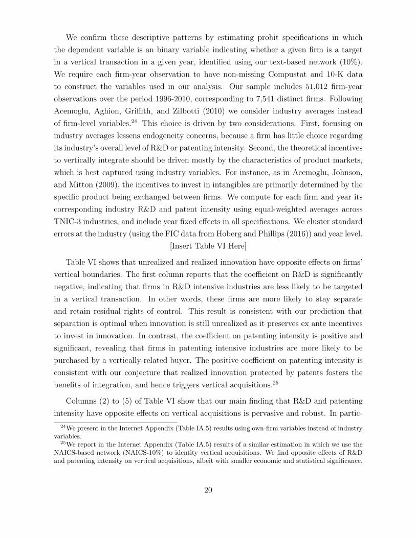
We confirm these descriptive patterns by estimating probit specifications in which

the dependent variable is an binary variable indicating whether a given firm is a target

in a vertical transaction in a given year, identified using our text-based network (10%).

We require each firm-year observation to have non-missing Compustat and 10-K data

to construct the variables used in our analysis. Our sample includes 51,012 firm-year

observations over the period 1996-2010, corresponding to 7,541 distinct firms. Following

Acemoglu, Aghion, Griffith, and Zilbotti (2010) we consider industry averages instead

of firm-level variables.24 This choice is driven by two considerations. First, focusing on

industry averages lessens endogeneity concerns, because a firm has little choice regarding

its industry’s overall level of R&D or patenting intensity. Second, the theoretical incentives

to vertically integrate should be driven mostly by the characteristics of product markets,

which is best captured using industry variables. For instance, as in Acemoglu, Johnson,

and Mitton (2009), the incentives to invest in intangibles are primarily determined by the

specific product being exchanged between firms. We compute for each firm and year its

corresponding industry R&D and patent intensity using equal-weighted averages across

TNIC-3 industries, and include year fixed effects in all specifications. We cluster standard

errors at the industry (using the FIC data from Hoberg and Phillips (2016)) and year level.

[Insert Table VI Here]

Table VI shows that unrealized and realized innovation have opposite effects on firms’

vertical boundaries. The first column reports that the coefficient on R&D is significantly

negative, indicating that firms in R&D intensive industries are less likely to be targeted

in a vertical transaction. In other words, these firms are more likely to stay separate

and retain residual rights of control. This result is consistent with our prediction that

separation is optimal when innovation is still unrealized as it preserves ex ante incentives

to invest in innovation. In contrast, the coefficient on patenting intensity is positive and

significant, revealing that firms in patenting intensive industries are more likely to be

purchased by a vertically-related buyer. The positive coefficient on patenting intensity is

consistent with our conjecture that realized innovation protected by patents fosters the

benefits of integration, and hence triggers vertical acquisitions.25

Columns (2) to (5) of Table VI show that our main finding that R&D and patenting

intensity have opposite effects on vertical acquisitions is pervasive and robust. In partic-

24We present in the Internet Appendix (Table IA.5) results using own-firm variables instead of industryvariables.

25We report in the Internet Appendix (Table IA.5) results of a similar estimation in which we use theNAICS-based network (NAICS-10%) to identity vertical acquisitions. We find opposite effects of R&Dand patenting intensity on vertical acquisitions, albeit with smaller economic and statistical significance.

20

ular, column (2) shows that our results persist after we control for additional variables

known to affect vertical integration that might also be correlated with R&D and patent

intensity, such as proxies for firms’ maturity (size, age, and market-to-book ratio), tan-

gibility (PPE over assets), the number of operating segments, the closeness to the end

of the supply chain (Final User), and industry concentration (HHI). In column (3), we

further include (broad) industry×year fixed effects (based on FIC-100 industries from

Hoberg and Phillips (2016)) to control for any time-varying industry characteristic, and

find similar results.

Our results are also robust to changes in the measurement of R&D and patenting

intensity. In column (4), we consider sales-weighted industry averages to account for the

potential variability of firms’ size within industries. In column (5), we use lagged values

for all independent variables. In column (6) we measure industry R&D and patenting

intensity directly from firms’ 10Ks to avoid potential measurement problems associated

with the reporting of R&D expenses in Compustat, and incomplete patent counts when

assigning patents to firms. Specifically, we count the number of paragraphs mentioning

R&D or patents in each 10K and scale these counts by the total number of paragraphs.26

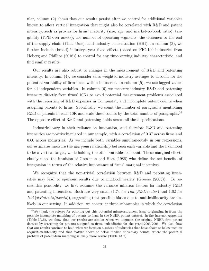
The opposite effect of R&D and patenting holds across all these specifications.

Industries vary in their reliance on innovation, and therefore R&D and patenting

intensities are positively related in our sample, with a correlation of 0.37 across firms and

0.60 across industries. As we include both variables simultaneously in our regressions,

our estimates measure the marginal relationship between each variable and the likelihood

to be a vertical target, while holding the other variables constant. These marginal effects

closely maps the intuition of Grossman and Hart (1986) who define the net benefits of

integration in terms of the relative importance of firms’ marginal incentives.

We recognize that the non-trivial correlation between R&D and patenting inten-

sities may lead to spurious results due to multicollinearity (Greene (2003)). To as-

sess this possibility, we first examine the variance inflation factors for industry R&D

and patenting intensities. Both are very small (1.74 for Ind.(R&D/sales) and 1.62 for

Ind.(#Patents/assets)), suggesting that possible biases due to multicollinearity are un-

likely in our setting. In addition, we construct three subsamples in which the correlation

26We thank the referee for pointing out this potential mismeasurement issue originating in from thepossible incomplete matching of patents to firms in the NBER patent dataset. In the Internet Appendix(Table IA.6), we show that our results are similar when we augment the original NBER firm-patentdataset by searching for patents assigned to firms’ subsidiaries for the years 2003-2006. We also showthat our results continue to hold when we focus on a subset of industries that have above or below medianacquisition-intensity and that feature above or below median subsidiary counts, where the potentialproblem of patent-firm matching is likely more severe (Table IA.7).

21

between R&D and patenting is small, thereby limiting the scope for multicollinearity prob-

lems. Every year, we independently assign observations into three, four, or five groups

based on tercile, quartile, or quintile splits for industry R&D and patenting intensity.

We then keep observations that are not assigned in similar groups (e.g. low tercile for

R&D and high tercile for patenting). This procedure thus generates subsamples featuring

correlations between R&D and patenting intensities of 0.01, 0.20, and 0.28 respectively.

Estimates obtained for these subsamples displayed in columns (7) to (9) are qualitatively

similar to our baseline estimates, mitigating the concern that our baseline results are

artificially inflated due to multicollinearity.27

C Contract Incompleteness and Hold Up Costs

To provide further support for our interpretation, we consider specialized predictions

regarding the economic mechanisms underlying our hypothesis. Our hypothesis is that

the stage of innovation matters in the formation of vertical firm boundaries through two

channels: incomplete contracting and the risk of hold up. Contracting incompleteness

incentivizes firms with unrealized innovation to remain separate in order to maintain

incentives to invest in relationship specific investment (Grossman and Hart (1986)). The

risk of hold up, in contrast, incentives firms to integrate in order to reduce the risk of

hold up and facilitate investment in commercialization (Williamson (1979)).

To test for the first channel, we create two measures of the difficulty to contract. Ti-

role (2016) argues that contract incompleteness can be measured as the frequency with

which contracts are disputed ex post, as this is a consequence of ex ante contract short-

comings. Our two measures are thus based on the intensity of litigations specifically

relating to contracts and innovation. Our measures are computed at the industry level

as this reduces the possible impact of endogeneity relating to the stage of innovation of

any specific firm. Our first measure is “Patent Infringement”, which we measure as the

number of paragraphs in a given firm’s 10-K that specifically discuss patent infringement.

This is identified using specific synonym-based word lists as in Hoberg and Maksimovic

(2015). We count the number of paragraphs that contain at least one word from each

27We report in the Internet Appendix two additional analyses. First, a bootstrap analysis in which were-estimate our baseline specification 1,000 times on sub-samples composed of 3,000 randomly selectedfirms indicates that our estimates are remarkably stable across samples (Figure IA.1). Second, we runregressions with patenting intensity and R&D intensity separately (Table IA.8), and find that patentingis always significant and positive, whereas R&D is negative and insignificant. The decrease in significanceof the R&D variable likely indicates that this variable partially pick up the omitted patenting intensityvariable, creating an omitted variable bias reducing the R&D intensity coefficient. This arises becausepatenting intensity is in fact a highly significant omitted variable.

22

of the following two lists: {patent, patents, patented} and {infringement, infringe}. Our

second measure is “Innovation Contract Litigation”, which we measure as the number of

paragraphs in a given firm’s 10-K that specifically discuss innovation contract litigation

using synonym-based word lists. In particular, we count the number of paragraphs that

contain at least one word from each of the three lists: {litigation, lawsuit, lawsuits},{contract, contracts, contractual}, and {patent, patents, patented, research, develop-

ment, trade secret, trade secrets, license, licenses, licensed, licensing, royalties, product,

products, service, services}. We average both measures over each firm’s TNIC peers to

generate industry exposures to patent infringement and innovation contract litigation.

To test the second channel, we create two measures of hold up risk. We follow Ace-

moglu, Aghion, Griffith, and Zilbotti (2010) and consider (1) the number of firms in the

given firm’s TNIC-3 industry and (2) the degree of industry concentration (we specifically

use the TNIC-3 industry’s Herfindahl index). The risk of hold up is expected to be high

when the first measure is low or when the second measure is high. In paraticular, these

variables capture the extent of a given firm’s outside options and thus its anticipated bar-

gaining power regarding the innovation. A lack of outside options makes it easier for firms

to behave opportunistically ex-post, increasing hold up risk for the user of the innovation.

We note that these variables are naturally computed at the industry level.

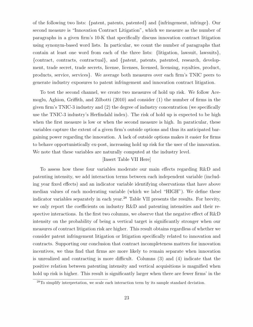
[Insert Table VII Here]

To assess how these four variables moderate our main effects regarding R&D and

patenting intensity, we add interaction terms between each independent variable (includ-

ing year fixed effects) and an indicator variable identifying observations that have above

median values of each moderating variable (which we label “HIGH”). We define these

indicator variables separately in each year.28 Table VII presents the results. For brevity,

we only report the coefficients on industry R&D and patenting intensities and their re-

spective interactions. In the first two columns, we observe that the negative effect of R&D

intensity on the probability of being a vertical target is significantly stronger when our

measures of contract litigation risk are higher. This result obtains regardless of whether we

consider patent infringement litigation or litigation specifically related to innovation and

contracts. Supporting our conclusion that contract incompleteness matters for innovation

incentives, we thus find that firms are more likely to remain separate when innovation

is unrealized and contracting is more difficult. Columns (3) and (4) indicate that the

positive relation between patenting intensity and vertical acquisitions is magnified when

hold up risk is higher. This result is significantly larger when there are fewer firms’ in the

28To simplify interpretation, we scale each interaction term by its sample standard deviation.

23

targets’ industry, and when the industry is more concentrated.

D Alternative Explanations

Our results so far are consistent with the hypothesis that firms’ vertical boundaries are

determined by the stage of innovation through the channels of incomplete contracting

and hold up risk. We recognize however that our results could potentially be consistent

with explanations unrelated to these mechanisms. We consider three possibilities. First,

despite the inclusions of a host of control variables and fixed effects, variables omitted

from our specification could still explain firms’ vertical organization and the R&D and

patenting intensity of their industries. For instance, industries’ R&D and patenting inten-

sities may correlate (in opposite directions) with time-varying unobserved variables linked

to integration, such as product life cycles, industries’ scope, or their natural tendency to

consolidate. Second, our results could reflect a story in which potential buyers use patent

grants as signals for innovation success, which increase expected synergies and trigger

acquisitions. Third, our findings could also be obtained under a “reverse-causality” sce-

nario in which firms respond to the likelihood of acquisitions by simultaneously reducing

R&D and increasing patenting. Several ancillary tests limit the scope for these alternative

explanations and reinforce our interpretation.

D.1 Falsification Test: Non-Vertical Acquisitions

First, we examine the link between the stage of development of innovation and non-

vertical acquisitions. Non-vertical transactions are relevant falsification events in our

setting. This is because the hypothesized effect of unrealized and realized innovation does

not clearly extend to other types of transactions such as horizontally related acquisitions

since the issues of ex-ante incentives, contracting difficulties, and potential hold up risk

are more specific to vertical relationships. Underscoring this prediction, theories based

on horizontal patent races predict that R&D intensive firms have higher incentives to

merge to internalize the effect of competition, and recent theories explaining horizontal

acquisitions emphasize asset complementarity and product market synergies.29

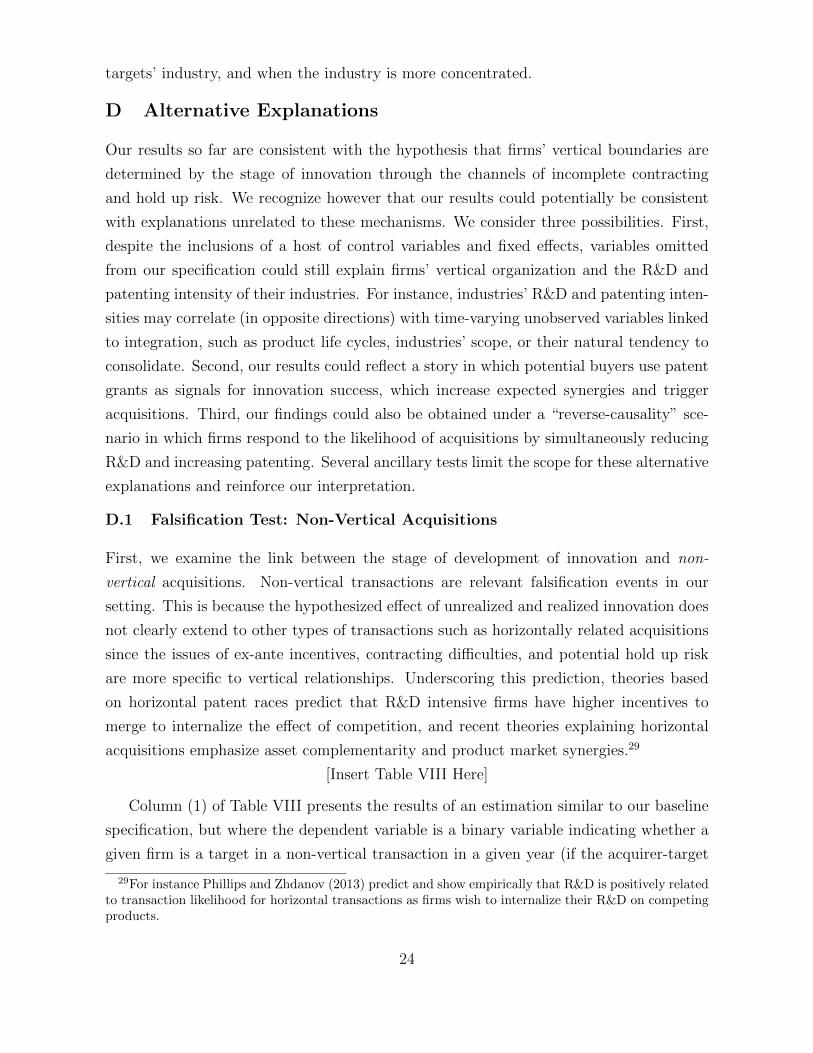
[Insert Table VIII Here]

Column (1) of Table VIII presents the results of an estimation similar to our baseline

specification, but where the dependent variable is a binary variable indicating whether a

given firm is a target in a non-vertical transaction in a given year (if the acquirer-target

29For instance Phillips and Zhdanov (2013) predict and show empirically that R&D is positively relatedto transaction likelihood for horizontal transactions as firms wish to internalize their R&D on competingproducts.

24

pair is not in our vertical text-based network. We find that the effect of unrealized and

realized innovation on non-vertical acquisitions is the mirror image to that of vertical

acquisitions. Firms in R&D intensive industries are more likely to be targets in non-

vertical acquisitions, whereas firms in high patenting industries are significantly less likely

to be purchased by a vertical buyer. The same results are obtained in column (2) where

we specifically focus on horizontal acquisitions, defined as transactions where acquirers

and targets are in the same industry (using the TNIC industries).

These patterns are confirmed in Figure 7 when we look at the average patenting and

R&D intensity of target firms prior to their acquisition. Vertical acquisitions tend to occur

after targets experience a period of increased patenting activity (either measured with the

(log of the) number of patents or using patenting intensity). The opposite appears true for

non-vertical acquisitions, which cluster after periods of low patenting activity. Although

the dynamics are less clear-cut for R&D, Figure 7 confirms that there are pervasive large

differences in R&D intensity between vertical and non-vertical targets.

Overall the negative link between R&D intensity and acquisitions appears unique to

vertical acquisitions. Consistent with recent evidence indicating that small firms conduct

more R&D when they face a high probability of selling out to larger horizontally related

firms, R&D intensity is positively related to non-vertical acquisitions. In addition, the

positive association between patenting intensity and acquisitions is only observed for

vertical acquisitions. These results provide additional evidence supporting our hypothesis

that vertical acquisitions are driven by the trade-off between ex-ante incentives and ex

post hold up risk. In addition, the stark differences between vertical and non-vertical

acquisitions mitigate concerns that our interpretation is counfonded by the presence of

unobserved industry characteristics (e.g., buyers using patents as a signal for innovation

success or industries’ natural tendency to consolidate). If it was the case, these omitted

characteristics should consistently explain all acquisitions.

D.2 Tax Credits as an Instrument for R&D intensity

We next consider a formal instrumental variables model following Bloom, Schankerman,

and van Reenen (2013), and we use tax-induced changes to the user cost of R&D to

construct an instrument for industry R&D intensity. State R&D tax credits offer firms

credits against state income tax liability based on the amount of qualified research done

within the state.30 The logic of our instrumental variable approach is as follows. By

30As detailed in Wilson (2009), state and federal tax credits are based on the amount of qualifiedresearch within the state or country. States generally follow the Federal Internal Revenue Code (IRC)definition of qualified research: the wages, material expenses, and rental costs of certain property and

25

offering tax credits for R&D expenses, states lower the user cost of R&D, which induce

firms to increase their R&D spending. Because they are largely random (see the dis-

cussion and evidence in Bloom, Schankerman, and van Reenen (2013)), these favorable

tax treatments generate variation in firms’ R&D that are purely tax-driven and hence

unrelated to their vertical organiztion. Tax credits thus represent exogenous shifts in the

margin of unrealized innovation. If, as we conjecture, vertical acquisitions are driven by

the distinction between unrealized and realized innovation, a positive exogenous shift in

unrealized innovation should encourage innovative firms to maintain their residual rights

of control, and favor separation over vertical integration.

To test this claim, we use the tax-induced user cost of R&D capital in state s and year

t (ρs,t) given by the Hall-Jorgenson formula:

ρs,t =1− (ks,t + kft )− (τs,t + τ ft )

1− (τs,t + τ ft )[rt + δ], (2)

where ks,t and kft are the state and federal R&D tax credit rates, τs,t and τ ft are the

state and federal corporation income tax rates, rt is the real interest rate, and δ is the

depreciation rate of R&D capital. The data are from Wilson (2009) and cover the period

1996-2006. In practice, states have different levels of R&D tax credits, and hence the user

cost of R&D is dependent on the location of firms’ R&D spending and time. Because we

do not know the state location of each firm’s R&D spending, we assume that all R&D

activities are performed in the firm’s headquarter state.31 Following the methodology of

Bloom, Schankerman, and van Reenen (2013), we implement the instrumental variable

model by first projecting each firm-year’s R&D intensity (R&D/sales) on the instrument

(ρ) as well as firm and year fixed effects.32 We then calculate the predicted R&D in-

tensity for each firm and year. Next, we average firms’ predicted R&D intensity across

each industry-year to create the instrument for industry R&D intensity (which we label

Ind.(PredictedR&D/sales)).

Columns (3) to (5) of Table VIII report results from the instrumental variables model.33

Column (3) presents the first-stage results. We observe a positive and highly significant

equipment incurred in performing research“undertaken to discover information” that is “technological innature” for a new or improved business purpose.

31We recognize that individual firm locations are not random, as some firms may have incentives tomove operations across states to reap larger R&D tax credits. Such moves can generate variation inindustry R&D intensity. Yet, to invalidate our instrumental variable strategy, one would have to arguethat mass relocations of firms in a given industry to exploit tax credits would have a direct effect on thepropensity of firms to be purchased by a vertically-related acquirer from a different industry. Althoughwe cannot formally rule out this explanation, we find it implausible.

32We show the results of this estimation in the Internet Appendix (Table IA.9).33Due to the binary nature of the dependent variable, we estimate instrumental variables using probit

26

coefficient on the industry tax-induced predicted R&D, indicating that industries where

more firms benefit from tax credits are indeed more R&D intensive. The second-stage

estimates reported in column (4) indicate that an increase in the instrumented R&D

intensity of a firm’s industry significantly reduces the likelihood that it is targeted by

a vertical buyer. Interestingly, and in contrast in column (5), we find that an increase

in instrumented R&D intensity leads to significantly more non-vertical acquisitions. To

the extent that the variation in industry R&D intensity driven by state tax credits is

exogenous, these results are difficult to reconcile with alternative explanations.

V Vertical Integration within Firms

To further test our hypothesis, we examine the effect of the stage of innovation on the

intensity of realized vertical integration within firms. We measure the extent to which

a given firm is “vertically integrated” by computing its degree of vertical relatedness

to itself. Using the notation from Section III, firm-level vertical integration is thus the

diagonal entries of the triple product in equation (3):

V Ii = [B · V ·B′]i,i. (3)

As illustrated in Figure 6, V I intuitively uses the vertical relatedness between com-

modity words from the BEA data (depicted in Figure 4) and examines the words in a

single firm’s business description to identify whether vertically related words jointly ap-

pear. The arrows indicate vertically related words in the firm’s 10-K. The more such links

exist for a given firm, the higher is the firm’s V I score. A firm is thus more vertically inte-

grated when its 10-K business description contains word pairs that are vertically related.

This occurs when a firm offers products or services at different stages of a specific supply

chain. In Figure 6, firm B is highly vertically integrated, and firm A is not integrated. In

the Internet Appendix, we provide strong evidence that validates that our measure of VI

indeed measures the extent to which firms are vertically integrated.34

A Patterns and Examples

Panel A of Table IX indicates that average value of vertical integration (V I) is 0.012, and

the maximum is 0.11. Although the nominal magnitudes do not have a direct interpre-

regressions using Maximum Likelihood. We obtain similar results if we use Linear Probability Models(see Table IA.10 of the Internet Appendix).

34Unfortunately, data limitations prevent us from determining the economic weight of each productfrom firms’ 10-K product descriptions. Hence, while V I is a novel measure that uniquely captures firm-level vertical integration, it cannot account for product-by-product importance.

27

tation, we note that there is a fair amount of right skewness. Most firms in our sample

are not vertically integrated. However, a smaller number of firms do feature business de-

scriptions that contain many words that are strongly vertically related. Hence, the firms

situated toward the right tail are likely the set of firms that are vertically integrated. Fig-

ure 9 displays the evolution of vertical integration over time, and we note a trend away

from integration especially in the late 1990s.35

[Insert Table IX Here]

Panel B of Table IX displays average statistics across quartiles of vertical integration.

Consistent with our central hypothesis, integrated firms spend less on R&D than non-

integrated firms. The average R&D intensity is roughly four times larger in low integration

quartiles than in the high integration quartiles (10.6% versus 2.7%). In contrast, vertically

integrated firms receive on average more patent grants. The (log) number of patent grants

is two times larger in the high integration quartile (0.848 versus 0.444).

The distinction between unrealized and realized innovation is exemplified by the net-

working equipment industry, which includes Cisco, Broadcom, Citrix, Juniper, Novell,

Sycamore, and Utstarcom. Figure 10 shows that these firms became four to five fold

more vertically integrated in our sample period. They also experienced (A) levels of R&D

that peaked in 2002 and then began to sharply decline, and (B) levels of patenting activity

that increased four to five fold starting in 2001. These dynamics are broadly consistent

with the idea that the conversion of unrealized innovation into realized patented innova-

tion increased the incentives to vertically integrate as the importance of residual rights of

control shifted from the smaller innovative firms to the larger commercializing firms.

B Stage of Innovation and Vertical Integration

Table X reports results from panel data regressions in which the dependent variable is

our measure of vertical integration (V Ii,t) measured for each firm and year. Confirm-

ing the univariate evidence, firms operating in industries that spend more on R&D are

significantly less vertically integrated. In sharp contrast, the coefficients on patenting

intensity are positive and significant. All else equal, firms operating in high patenting

industries are more likely to be vertically integrated. Both main results are robust both

within industries (when we include industry fixed effects in column (1)) and within firms

35In the Internet Appendix (Table IA.11), we further illustrate our text-based measure of verticalintegration by displaying the 30 most vertically integrated firms in 2008. A close look at these firmssuggests a high degree of actual vertical relatedness among product offerings. Moreover, although theyare highly integrated, these firms rank rather low on existing non-text measures of integration based onCompustat segments.

28

(with firm fixed effects in column (2)). The latter result is particularly important as the

inclusion of firm fixed effects absorbs any time-invariant firm characteristics (e.g., inno-

vative culture or unobserved quality). It further indicates that firms modify their degree

of vertical integration over time in response to changes in industry R&D and patenting

intensity. Several alternative specifications reported in the Internet Appendix confirm the

robustness of these results.36

[Insert Table X Here]

Economically, the effects of unrealized and realized innovation on integration is sub-

stantial. A one standard deviation increase in R&D intensity is associated with a 9.5%

decrease in integration in the within-industry specification, and a 2.2% decrease in the

within-firm specification.37 Analogously, vertical integration increases by 8% (2.7%) fol-

lowing a one standard deviation increase in patenting intensity in the within-industry

(within-firm) specification.

Columns (3) to (6) of Table X examine the sensitivity of these results to increases in

our measures of contract incompleteness and hold up risk. For brevity, we only report

results from specifications that include firm fixed effects. Mirroring the results reported

in Table VII, we observe in columns (3) and (4) that the interaction between R&D and

HIGH is negative and significant. We conclude that the negative association between

R&D intensity and vertical integration is stronger when industry patent infringement lit-

igation and industry innovation contract litigation intensity are higher. These results are

consistent with firms favoring separation when innovation is unrealized and contracting

is difficult. In contrast, columns (5) and (6) reveal that the positive sensitivity of vertical

integration to patenting intensity increases with measures of industry hold up risk. Ver-

tical integration is thus favored when innovation is realized and hold up risk is higher.

Finally, the last column of Table X reports instrumental variables tests using our measure

of predicted industry R&D/sales based on tax credits as an instrument for industry R&D

intensity. We continue to observe a negative and significant coefficient on instrumented

industry R&D, indicating that lower levels of vertical integration at the firm-level arise

when unrealized innovation exogenously increases.

Overall, results in Table X corroborate our central hypothesis. Vertical integration

decreases when innovation is unrealized consistent with lower integration preserving in-

vestment incentives. Firms are more vertically integrated when innovation is realized con-

36In particular, Table IA.12 shows that the results are robust to different measurement of R&D andpatenting intensity, multicollinearity concerns, and using the log of V I as the dependent variable.

37The lower magnitude within-firm reflects the high degree of persistence of V I at the firm-level. Thecoefficient of autocorrelation for V I is 0.931.

29

sistent with commercialization incentives and reducing hold up risk. Remarkably, these

results obtain even when we control for unobserved firm characteristics, in instrumental

variables tests, and when we examine predictions specific to these proposed mechanisms.

VI Conclusions

Our paper examines vertical acquisitions and changes in firm-specific vertical integration.

We consider theoretical predictions regarding how incentives to invest in R&D, and the

potential for ex post holdup, influence vertical transactions and integration. We measure

vertical relatedness using computational linguistics analysis of firm product descriptions

and how they relate to product vocabularies from the BEA Input-Output tables. The

result is a dynamic network of vertical relatedness between publicly-traded firms. We thus

observe the extent to which acquisitions are vertical transactions and develop a new firm-

level measure of vertical integration. This new text-based measure of vertical integration

links both BEA product vocabulary and firm 10-K vocabulary to be able to ascertain

how firms are vertically organized. It adds to the growing literature using text as data in

economics, recently surveyed by Gentzkow, Kelly, and Taddy (2017).

We show that unrealized innovation through R&D, and realized innovation through

patents, impact the propensity to vertically integrate in opposite ways. Firms in R&D

intensive industries are less likely to vertically integrate through own-production and

vertical acquisitions. These results are stronger when measures of contracting litigation

risk are higher and are robust to using state-level tax credits as an instrument for R&D

expenses. Our findings are consistent with firms remaining separate to maintain ex ante

incentives to invest in intangible capital and to maintain residual rights of control, as in

the property rights theory of Grossman, Hart and Moore.

In contrast, firms in patenting intensive industries with high realized innovation and

high measures of competition are more likely to vertically integrate. In these industries,

owners have more legally enforceable residual rights of control. They are more likely to

integrate via acquisitions because giving control to commercializing firms should mitigate

ex post holdup. These results reconcile some of the tension between the ex post hold-up

literature of Klein, Crawford, and Alchian (1978) and Williamson (1979), and the ex ante

property rights literature of Grossman and Hart (1986)) and Hart and Moore (1990)),

which emphasizes the incentive effects of assigning residual rights of control.

30

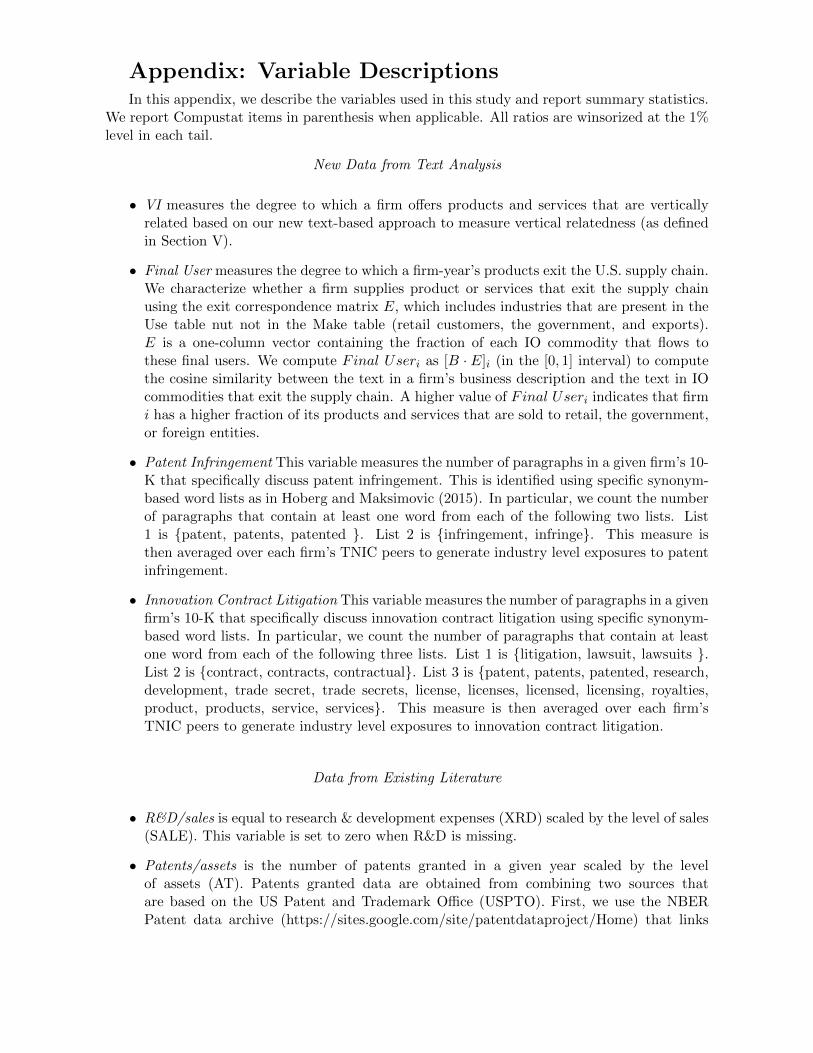
Appendix: Variable DescriptionsIn this appendix, we describe the variables used in this study and report summary statistics.

We report Compustat items in parenthesis when applicable. All ratios are winsorized at the 1%level in each tail.

New Data from Text Analysis

• VI measures the degree to which a firm offers products and services that are verticallyrelated based on our new text-based approach to measure vertical relatedness (as definedin Section V).

• Final User measures the degree to which a firm-year’s products exit the U.S. supply chain.We characterize whether a firm supplies product or services that exit the supply chainusing the exit correspondence matrix E, which includes industries that are present in theUse table nut not in the Make table (retail customers, the government, and exports).E is a one-column vector containing the fraction of each IO commodity that flows tothese final users. We compute Final Useri as [B · E]i (in the [0, 1] interval) to computethe cosine similarity between the text in a firm’s business description and the text in IOcommodities that exit the supply chain. A higher value of Final Useri indicates that firmi has a higher fraction of its products and services that are sold to retail, the government,or foreign entities.

• Patent Infringement This variable measures the number of paragraphs in a given firm’s 10-K that specifically discuss patent infringement. This is identified using specific synonym-based word lists as in Hoberg and Maksimovic (2015). In particular, we count the numberof paragraphs that contain at least one word from each of the following two lists. List1 is {patent, patents, patented }. List 2 is {infringement, infringe}. This measure isthen averaged over each firm’s TNIC peers to generate industry level exposures to patentinfringement.

• Innovation Contract Litigation This variable measures the number of paragraphs in a givenfirm’s 10-K that specifically discuss innovation contract litigation using specific synonym-based word lists. In particular, we count the number of paragraphs that contain at leastone word from each of the following three lists. List 1 is {litigation, lawsuit, lawsuits }.List 2 is {contract, contracts, contractual}. List 3 is {patent, patents, patented, research,development, trade secret, trade secrets, license, licenses, licensed, licensing, royalties,product, products, service, services}. This measure is then averaged over each firm’sTNIC peers to generate industry level exposures to innovation contract litigation.

Data from Existing Literature

• R&D/sales is equal to research & development expenses (XRD) scaled by the level of sales(SALE). This variable is set to zero when R&D is missing.

• Patents/assets is the number of patents granted in a given year scaled by the levelof assets (AT). Patents granted data are obtained from combining two sources thatare based on the US Patent and Trademark Office (USPTO). First, we use the NBERPatent data archive (https://sites.google.com/site/patentdataproject/Home) that links

granted patents to publicly-traded firms (based on firms’ GVKEY) until 2006. Second,we use the patent dataset developed by Kogan, Papanikolaou, Seru, and Stoffman (2016)(https://iu.app.box.com/v/patents) that complements the NBER dataset by enhancingthe matching to GVKEY and extending the sample to 2010. Table IA.13 of the InternetAppendix details the composition of our patent sample.

• PPE/assets is equal to the level of property, plant and equipment (PPENT) divided bytotal assets (AT).

• HHI measures the degree of concentration (of sales) within TNIC-3 industries. We com-pute HHI as the TNIC-3 HHI in Hoberg and Phillips (2016), which is based on thetext-based TNIC-3 horizontal industry network.

• Log(assets) is the natural logarithm of the firm assets (AT).

• Log(age) is the natural logarithm of one plus the firm age. Age is computed as the currentyear minus the firm’s founding date. When we cannot identify a firm’s founding date, weuse its listing vintage (based on the first year the firm appears in the Compustat database).

• Segments is the number of operating segments observed for the given firm in the Compustatsegment database. We measure operating segments based on the NAICS classification.

• MB is the firm’s market-to-book ratio. It is computed as total assets (TA) minus commonequity (CEQ) plus the market value of equity ((CSHO×PRCC F)) divided by total assets.

• VIsegment measures firm-level vertical integration based on Compustat Segments. It iscomputed as the average vertical relatedness across a firm’s distinct NAICS segments.Vertical relatedness is based on the matrix Z (defined in Section III.D ) that relies on the2002 BEA Input-Output table.

• Peers measures the number of firms in each firm’s TNIC-3 horizontal network.

• User cost of R&D capital (ρ) is the user cost of R&D capital in state s and year t is given

by the Hall-Jorgenson formula:ρs,t =1−(ks,t+k

ft )−(τs,t+τ

ft )

1−(τs,t+τft )

[rt+ δ], where ks,t and kft are the

state and federal R&D tax credit rates, τs,t and τ ft are the state and federal corporationincome tax rates, rt is the real interest rate, and δ is the depreciation rate of R&D capital.The data are from Wilson (2009) and cover the period 1996-2006.

Table A1: Summary Statistics

Variable: Mean St. Dev Min Max #Obs.

Panel A: Data from Text Analysis

VI 0.012 0.011 0 0.11 51,012

Final User 0.469 0.076 0.086 0.973 51,012

Patent Infringement 1.271 3.121 0 73 51,012

Innovation Contract Litigation 0.272 0.744 0 14 51,012

Panel B: Data from Existing Literature

R&D/sales 0.062 0.134 0 0.785 51,012

Patents/assets 0.008 0.022 0 0.136 51,012

log(Patents) 0.619 1.203 0 8.529 51,012

PPE/assets 0.263 0.224 0.009 0.896 51,012

HHI 0.229 0.189 0.015 0.999 51,012

log(assets) 5.748 1.785 2.461 10.288 51,012

log(age) 2.908 1.104 0 4.997 51,012

Segments 1.532 0.976 1 12 51,012

MB 1.97 1.452 0.589 8.736 51,012

VI(segment) 0.013 0.037 0 0.639 51,012

Peers 50.92 58.82 1 497 51,012

Use cost of R&D capital 1.168 0.041 1.028 1.238 39,553

Note: This table displays summary statistics for all the variables used in the analysis.

References

Acemoglu, Daron, 1996, A microfoundation for social increasing returns in human capital accumulation,Quarterly Journal of Economics 111, 779–804.

, Phillipe Aghion, Rachel Griffith, and Fabrizio Zilbotti, 2010, Vertical integration and technology:Theory and evidence, Journal of the European Economic Association pp. 989–1033.

Acemoglu, Daron, Simon Johnson, and Todd Mitton, 2009, Determinants of vertical integration: Finan-cial development and contracting costs, Journal of Finance 64, 1251–1290.

Aghion, Philippe, and Jean Tirole, 1994, The management of innovation, Quarterly Journal of Economicspp. 1185–1209.

Ahern, Kenneth, 2012, Bargaining power and industry dependence in mergers, JFE 103, 530–550.

, and Jarrad Harford, 2013, The importance of industry links in merger waves, Journal of Finance(forthcoming) University of Michigan and University of Washington Working Paper.

Antweiler, Werner, and Murray Frank, 2004, Is all that talk just noise? the information content ofinternet stock message boards, Journal of Finance 52, 1259–1294.

Atalay, Enghin, Ali Hortacsu, and Chad Syverson, 2014, Vertical integration and input flows, AmericanEconomic Review pp. 1120–1148.

Baker, Geroge, and Thomas Hubbard, 2003, Make versus buy in trucking: Asset ownership, job design,and information, American Economic Review pp. 551–572.

Bena, Jan, and Kai Li, 2013, Corporate innovations and mergers and acquisitions, Journal of Finance(forthcoming).

Bloom, Nicholas, Mark Schankerman, and John van Reenen, 2013, Identifying technology spillovers andproduct market rivalry, Econometrica pp. 1347–1393.

Bresnahan, Timothy, and Jonathan Levin, 2012, Vertical integration and market structure, WorkingPaper.

Fan, Joseph, and Vidhan Goyal, 2006, On the patterns and wealth effects of vertical mergers, Journal ofBusiness 79, 877–902.

Gentzkow, Matthew, Brian Kelly, and Matt Taddy, 2017, Text as data, University of Chicago workingpaper.

Gentzkow, Matthew, and Jesse M. Shapiro, 2010, What drives media slant? evidence from us dailynewspapers, Econometrica 78, 35–71.

Gibbons, Robert, 2005, Four formal(izable) theories of the firm?, Journal of Economic Behavior andOrganization 58, 200–245.

Greene, William, 2003, Econometrics Analysis (Prentice Hall).

Groseclose, Tim, and Jeffrey Milyo, 2005, A measure of media bias, The Quarterly Journal of Economics120, 1191–1237.

Grossman, Sanford J., and Oliver D. Hart, 1986, The cost and benefits of ownership: A theory of verticaland lateral integration, Journal of Political Economy 94, 691–719.

Harford, Jarrad, 2005, What drives merger waves?, Journal of Financial Economics 77, 529–560.

Hart, Oliver, and John Moore, 1990, Property rights and the nature of the firm, Journal of PoliticalEconomy 98, 1119–1158.

Hoberg, Gerard, and Vojislav Maksimovic, 2015, Redefining financial constraints: A text-based analysis,Review of Financial Studies 28, 1312–1352.

Hoberg, Gerard, and Gordon Phillips, 2010, Product market synergies in mergers and acquisitions: Atext based analysis, Review of Financial Studies 23, 3773–3811.

, 2016, Text-based network industry classifications and endogenous product differentiation, Jour-nal of Political Economy 124, 1423–1465.

Holmstrom, Bengt, and Paul Milgrom, 1991, Multi-task principal-agent problems: Incentive contracts,asset ownership and job design, Journal of Law, Economics and Organization 7, 24–52.

, 1994, The firm as an incentive system, American Economic Review 84, 972–991.

Hortacsu, Ali, and Chad Syverson, 2007, Cementing relationships: Vertical integration, foreclosure, pro-ductivity and prices, Journal of Political Economy pp. 250–301.

Joskow, Paul L., 1987, Contract duration and relationship specific investments, American EconomicReview 77, 168–175.

Jovanovic, Boyan, and P Rousseau, 2002, The q-theory of mergers, American Economic Review 92,198–204.

Kedia, Simi, Abraham Ravid, and Vicente Pons, 2011, When do vertical mergers create value?, FinancialManagement 40, 845–877.

Klein, Benjamin, Robert G. Crawford, and Armen A. Alchian, 1978, Vertical integration, appropriablerents, and the competitive contracting process, Journal of Law and Economics 21, 297–326.

Kogan, Leonid, Dimtris Papanikolaou, Amit Seru, and Noah Stoffman, 2016, Technological innovation,resource allocation and growth, Quarterly Journal of Economics forthcoming.

Lafontaine, Francine, and Margaret Slade, 2007, Vertical integration and firm boudaries: The evidence,Journal of Economic Literature 45, 629–685.

Maksimovic, Vojislav, and Gordon Phillips, 2001, The market for corporate assets: Who engages inmergers and asset sales and are there efficiency gains?, Journal of Finance 56, 2019–2065.

Masten, Scott E., 1984, The organization of production: Evidence from the aerospace industry, Journalof Law and Economics 27, 403–417.

Monteverde, Kirk, and David J. Teece, 1982, Supplier switching costs and vertical integration in automobilindustry, Bell Journal of Economics 13, 206–213.

Morck, Randall, Andrei Shleifer, and Robert Vishny, 1990, Do managerial motives drive bad acquisitions,Journal of Finance 45, 31–48.

Phillips, Gordon M., and Alexei Zhdanov, 2013, R&d and the incentives from merger and acquisitionactivity, Review of Financial Studies 34-78, 189–238.

Sebastiani, Fabrizio, 2002, Machine learning in automated text categorization, ACMCS 34, 1–47.

Seru, Amit, 2014, Firm boundaries matter: Evidence from conglomerates and r&d activity, Journal ofFinancial Economics 111, 381–405.

Tetlock, Paul C., 2007, Giving content to investor sentiment: The role of media in the stock market,Journal of Finance 62, 1139–1168.

Tirole, Jean, 2016, Remarks on incomplete contracting, in The Impact of Incomplete Contracts on Eco-nomics . chap. 3, pp. 21–25 (Oxford University Press).

Williamson, Olivier E., 1971, The vertical integration of production: Market failure consideration, Amer-ican Economic Review 61, 112–123.

, 1979, Transaction-cost economics: The governance of contractual relations, Journal of Law andEconomics 22, 233–261.

Wilson, Daniel, 2009, Beggar thy neighbor? the in-state, out-of-state, and aggregate effects of r&d taxcredits, Review of Economics and Statistics pp. 431–436.

Table I: BEA vocabulary example: Photographic and Photocopying Equipment

Description of Commodity Sub-Category Value of Production ($Mil.)

Still cameras (hand-type cameras, process cameras for photoengraving 266.1

and photolithography, and other still cameras)

Projectors 72.4

Still picture commercial-type processing equipment for film 40.5

All other still picture equipment, parts, attachments, and accessories 266.5

Photocopying equipment, including diffusion transfer, dye transfer, 592.4

electrostatic, light and heat sensitive types, etc.

Microfilming, blueprinting, and white-printing equipment 20.7

Motion picture equipment (all sizes 8mm and greater) 149.0

Projection screens (for motion picture and/or still projection) 204.9

Motion picture processing equipment 23.0

Processed commodity vocabulary: microfilming, whiteprinting, blueprinting, interchangeable, film, projectors, rear, viewers, screen, mm, photoengraving, photolithography, cameras, photographic, motion, electrostatic, diffusion, dye, heat, projection, screens, picture, still, photocopying

Note: This table provides an example of the BEA commodity ‘photographic and photocopying equipment’ (IOCommodity Code #333315). The table displays its sub-commodities and their associated product text, along with thevalue of production for each sub-commodity.

Table II: Vertical Network Summary Statistics

Network: Vert. Text-10% Vert. Text-1% NAICS-10% NAICS-1% TNIC-3

Granularity 10% 1% 9.28% 1.34% 2.33%

% of pairs in TNIC-3 1.53% 2.64% 2.76% 3.27% 100%

% of pairs in the same SIC 0.75% 1.01% 0.34% 0.17% 37.14%

% of pairs in the same NAICS 0.57% 0.58% 0.12% 0.11% 36.89%

% of pairs in the same SIC or NAICS 0.82% 1.07% 0.34% 0.17% 40.26%

% of pairs in Vert. Text-10% 100% 100% 10.43% 13.14% 6.82%

% of pairs in Vert. Text-1% 10% 100% 1.18% 1.16% 1.17%

% of pairs that include a financial firm 9.80% 2.10% 50.07% 35.97% 56.56%

% of (no fin.) pairs in Vert. Text-10% 100% 100% 19.67% 20.00% 11.63%

% of (no fin.) pairs in Vert. Text-1% 10% 100% 2.34% 1.80% 2.44%

Note: This table displays various characteristics for five networks: Vertical Text-10% and Vertical Text-1% verticalnetworks, NAICS-10% and NAICS-1% vertical networks, and the TNIC-3 horizontal network.

Table III: Validation: Vertical Integration Detection

Dep. Variable: Prob(V Isearch = 1)

(1) (2) (3) (4) (5) (6)

V I 0.217a 0.229a 0.125a 0.133a

(0.007) (0.007) (0.010) (0.010)

V Isegment 0.066a 0.101a 0.053a 0.064a

(0.007) (0.006) (0.008) (0.008)

Year FE No No No Yes Yes Yes

Industry FE No No No Yes Yes Yes

#.Obs. 51,012 51,012 51,012 51,012 51,012 51,012

Pseudo R2 0.038 0.035 0.008 0.131 0.130 0.126

Note: This table reports Probit estimations where the dependent variable is V Isearch, a dummy that equals one if a firmmentions being vertically integrated in its annual 10-K report, and zero otherwise. The independent variables arestandardized for convenience. Standard errors are clustered by industry and year and are reported in parentheses.Symbols a, b, and c indicate statistical significance at the 1%, 5%, and 10% confidence levels.

Table IV: Mergers and Acquisitions - Sample Description

Measure: All Text-Based NAICS-based

Deal type: Vertical Non-Vertical Vertical Non-Vertical

Panel A: Sample Description

# Transactions 4,377 1,741 2,636 579 3,828

% Vertical (Non-Vertical) 39.78% 60.22% 12.54% 87.46%

# Upstream 852 229

# Downstream 889 320

Panel B: Combined Acquirers and Targets Returns

CAR(0) 0.53% 0.64% 0.45% 0.41% 0.54%

CAR(-1,1) 0.79% 0.94% 0.69% 0.23% 0.87%

# Transactions 4,082 1,634 2,448 505 3,577

Note: Panel A displays statistics for vertical and non-vertical transactions (non-financial firms only). A transaction isvertical if the acquirer and target are pairs in the Vertical Text-10% network or the NAICS-10% network. Panel Bdisplays the average cumulated abnormal announcement returns (CARs) of combined acquirers and targets.

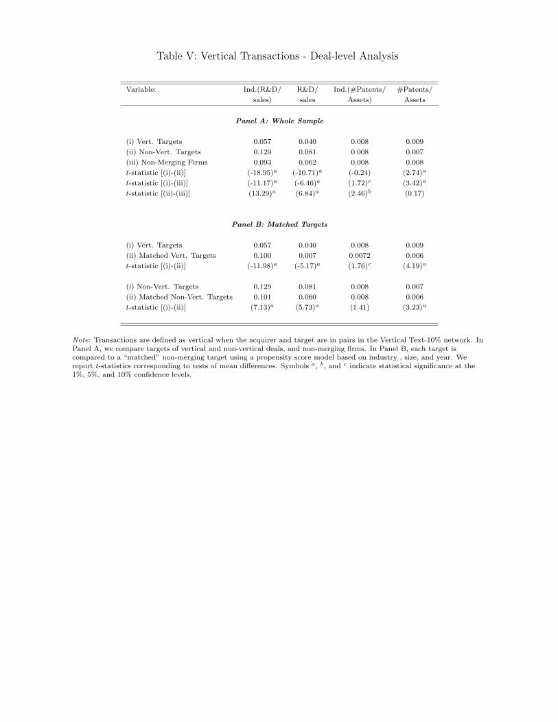
Table V: Vertical Transactions - Deal-level Analysis

Variable: Ind.(R&D/ R&D/ Ind.(#Patents/ #Patents/

sales) sales Assets) Assets

Panel A: Whole Sample

(i) Vert. Targets 0.057 0.040 0.008 0.009

(ii) Non-Vert. Targets 0.129 0.081 0.008 0.007

(iii) Non-Merging Firms 0.093 0.062 0.008 0.008

t-statistic [(i)-(ii)] (-18.95)a (-10.71)a (-0.24) (2.74)a

t-statistic [(i)-(iii)] (-11.17)a (-6.46)a (1.72)c (3.42)a

t-statistic [(ii)-(iii)] (13.29)a (6.84)a (2.46)b (0.17)

Panel B: Matched Targets

(i) Vert. Targets 0.057 0.040 0.008 0.009

(ii) Matched Vert. Targets 0.100 0.007 0.0072 0.006

t-statistic [(i)-(ii)] (-11.98)a (-5.17)a (1.76)c (4.19)a

(i) Non-Vert. Targets 0.129 0.081 0.008 0.007

(ii) Matched Non-Vert. Targets 0.101 0.060 0.008 0.006

t-statistic [(i)-(ii)] (7.13)a (5.73)a (1.41) (3.23)a

Note: Transactions are defined as vertical when the acquirer and target are in pairs in the Vertical Text-10% network. InPanel A, we compare targets of vertical and non-vertical deals, and non-merging firms. In Panel B, each target iscompared to a “matched” non-merging target using a propensity score model based on industry , size, and year. Wereport t-statistics corresponding to tests of mean differences. Symbols a, b, and c indicate statistical significance at the1%, 5%, and 10% confidence levels.

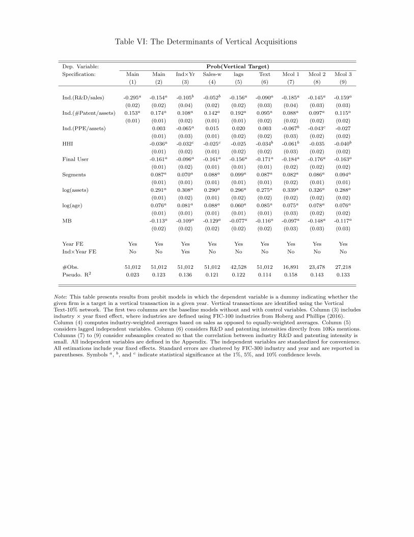
Table VI: The Determinants of Vertical Acquisitions

Dep. Variable: Prob(Vertical Target)

Specification: Main Main Ind×Yr Sales-w lags Text Mcol 1 Mcol 2 Mcol 3

(1) (2) (3) (4) (5) (6) (7) (8) (9)

Ind.(R&D/sales) -0.295a -0.154a -0.105b -0.052b -0.156a -0.090a -0.185a -0.145a -0.159a

(0.02) (0.02) (0.04) (0.02) (0.02) (0.03) (0.04) (0.03) (0.03)

Ind.(#Patent/assets) 0.153a 0.174a 0.108a 0.142a 0.192a 0.095a 0.088a 0.097a 0.115a

(0.01) (0.01) (0.02) (0.01) (0.01) (0.02) (0.02) (0.02) (0.02)

Ind.(PPE/assets) 0.003 -0.065a 0.015 0.020 0.003 -0.067b -0.043c -0.027

(0.01) (0.03) (0.01) (0.02) (0.02) (0.03) (0.02) (0.02)

HHI -0.036a -0.032c -0.025c -0.025 -0.034b -0.061b -0.035 -0.040b

(0.01) (0.02) (0.01) (0.02) (0.02) (0.03) (0.02) (0.02)

Final User -0.161a -0.096a -0.161a -0.156a -0.171a -0.184a -0.176a -0.163a

(0.01) (0.02) (0.01) (0.01) (0.01) (0.02) (0.02) (0.02)

Segments 0.087a 0.070a 0.088a 0.099a 0.087a 0.082a 0.086a 0.094a

(0.01) (0.01) (0.01) (0.01) (0.01) (0.02) (0.01) (0.01)

log(assets) 0.291a 0.308a 0.290a 0.296a 0.275a 0.339a 0.326a 0.288a

(0.01) (0.02) (0.01) (0.02) (0.02) (0.02) (0.02) (0.02)

log(age) 0.076a 0.081a 0.088a 0.060a 0.085a 0.075a 0.078a 0.076a

(0.01) (0.01) (0.01) (0.01) (0.01) (0.03) (0.02) (0.02)

MB -0.113a -0.109a -0.129a -0.077a -0.116a -0.097a -0.148a -0.117a

(0.02) (0.02) (0.02) (0.02) (0.02) (0.03) (0.03) (0.03)

Year FE Yes Yes Yes Yes Yes Yes Yes Yes Yes

Ind×Year FE No No Yes No No No No No No

#Obs. 51,012 51,012 51,012 51,012 42,528 51,012 16,891 23,478 27,218

Pseudo. R2 0.023 0.123 0.136 0.121 0.122 0.114 0.158 0.143 0.133

Note: This table presents results from probit models in which the dependent variable is a dummy indicating whether thegiven firm is a target in a vertical transaction in a given year. Vertical transactions are identified using the VerticalText-10% network. The first two columns are the baseline models without and with control variables. Column (3) includesindustry × year fixed effect, where industries are defined using FIC-100 industries from Hoberg and Phillips (2016).Column (4) computes industry-weighted averages based on sales as opposed to equally-weighted averages. Column (5)considers lagged independent variables. Column (6) considers R&D and patenting intensities directly from 10Ks mentions.Columns (7) to (9) consider subsamples created so that the correlation between industry R&D and patenting intensity issmall. All independent variables are defined in the Appendix. The independent variables are standardized for convenience.All estimations include year fixed effects. Standard errors are clustered by FIC-300 industry and year and are reported inparentheses. Symbols a, b, and c indicate statistical significance at the 1%, 5%, and 10% confidence levels.

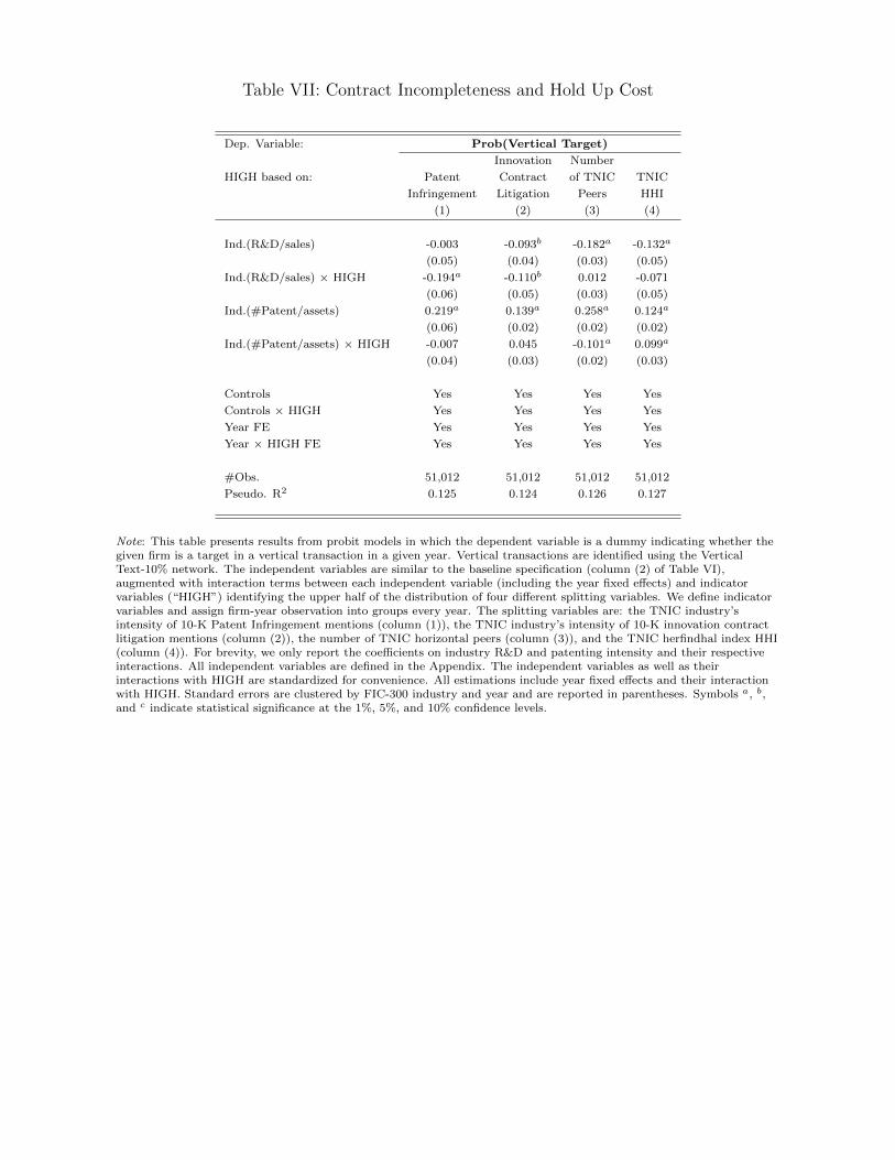
Table VII: Contract Incompleteness and Hold Up Cost

Dep. Variable: Prob(Vertical Target)

Innovation Number

HIGH based on: Patent Contract of TNIC TNIC

Infringement Litigation Peers HHI

(1) (2) (3) (4)

Ind.(R&D/sales) -0.003 -0.093b -0.182a -0.132a

(0.05) (0.04) (0.03) (0.05)

Ind.(R&D/sales) × HIGH -0.194a -0.110b 0.012 -0.071

(0.06) (0.05) (0.03) (0.05)

Ind.(#Patent/assets) 0.219a 0.139a 0.258a 0.124a

(0.06) (0.02) (0.02) (0.02)

Ind.(#Patent/assets) × HIGH -0.007 0.045 -0.101a 0.099a

(0.04) (0.03) (0.02) (0.03)

Controls Yes Yes Yes Yes

Controls × HIGH Yes Yes Yes Yes

Year FE Yes Yes Yes Yes

Year × HIGH FE Yes Yes Yes Yes

#Obs. 51,012 51,012 51,012 51,012

Pseudo. R2 0.125 0.124 0.126 0.127

Note: This table presents results from probit models in which the dependent variable is a dummy indicating whether thegiven firm is a target in a vertical transaction in a given year. Vertical transactions are identified using the VerticalText-10% network. The independent variables are similar to the baseline specification (column (2) of Table VI),augmented with interaction terms between each independent variable (including the year fixed effects) and indicatorvariables (“HIGH”) identifying the upper half of the distribution of four different splitting variables. We define indicatorvariables and assign firm-year observation into groups every year. The splitting variables are: the TNIC industry’sintensity of 10-K Patent Infringement mentions (column (1)), the TNIC industry’s intensity of 10-K innovation contractlitigation mentions (column (2)), the number of TNIC horizontal peers (column (3)), and the TNIC herfindhal index HHI(column (4)). For brevity, we only report the coefficients on industry R&D and patenting intensity and their respectiveinteractions. All independent variables are defined in the Appendix. The independent variables as well as theirinteractions with HIGH are standardized for convenience. All estimations include year fixed effects and their interactionwith HIGH. Standard errors are clustered by FIC-300 industry and year and are reported in parentheses. Symbols a, b,and c indicate statistical significance at the 1%, 5%, and 10% confidence levels.

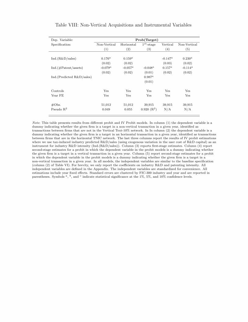
Table VIII: Non-Vertical Acquisitions and Instrumental Variables

Dep. Variable: Prob(Target)

Specification: Non-Vertical Horizontal 1st-stage Vertical Non-Vertical

(1) (2) (3) (4) (5)

Ind.(R&D/sales) 0.176a 0.159a -0.147a 0.230a

(0.02) (0.02) (0.03) (0.02)

Ind.(#Patent/assets) -0.079a -0.057a -0.048a 0.157a -0.114a

(0.02) (0.02) (0.01) (0.02) (0.02)

Ind.(Predicted R&D/sales) 0.987a

(0.01)

Controls Yes Yes Yes Yes Yes

Year FE Yes Yes Yes Yes Yes

#Obs. 51,012 51,012 39,915 39,915 39,915

Pseudo R2 0.049 0.055 0.920 (R2) N/A N/A

Note: This table presents results from different probit and IV Probit models. In column (1) the dependent variable is adummy indicating whether the given firm is a target in a non-vertical transaction in a given year, identified astransactions between firms that are not in the Vertical Text-10% network. In In column (2) the dependent variable is adummy indicating whether the given firm is a target in an horizontal transaction in a given year, identified as transactionsbetween firms that are in the horizontal TNIC network. The last three columns report the results of IV probit estimationswhere we use tax-induced industry predicted R&D/sales (using exogenous variation in the user cost of R&D capital) as aninstrument for industry R&D intensity (Ind.(R&D/sales)). Column (3) reports first-stage estimates. Column (4) reportsecond-stage estimates for a probit in which the dependent variable in the probit models is a dummy indicating whetherthe given firm is a target in a vertical transaction in a given year. Column (5) report second-stage estimates for a probitin which the dependent variable in the probit models is a dummy indicating whether the given firm is a target in anon-vertical transaction in a given year. In all models, the independent variables are similar to the baseline specification(column (2) of Table VI). For brevity, we only report the coefficients on industry R&D and patenting intensity. Allindependent variables are defined in the Appendix. The independent variables are standardized for convenience. Allestimations include year fixed effects. Standard errors are clustered by FIC-300 industry and year and are reported inparentheses. Symbols a, b, and c indicate statistical significance at the 1%, 5%, and 10% confidence levels.

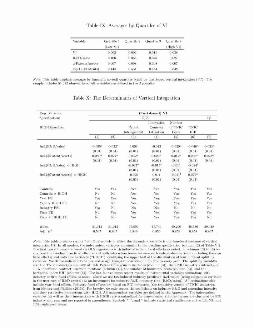
Table IX: Averages by Quartiles of VI

Variable Quartile 1 Quartile 2 Quartile 3 Quartile 4

(Low VI) (High VI)

VI 0.002 0.006 0.011 0.028

R&D/sales 0.106 0.065 0.048 0.027

#Patents/assets 0.007 0.008 0.008 0.007

log(1+#Patents) 0.444 0.531 0.654 0.848

Note: This table displays averages by (annually sorted) quartiles based on text-based vertical integration (V I). Thesample includes 51,012 observations. All variables are defined in the Appendix.

Table X: The Determinants of Vertical Integration

Dep. Variable: (Text-based) VI

Specification: OLS IV

Innovation Number

HIGH based on: Patent Contract of TNIC TNIC

Infringement Litigation Peers HHI

(1) (2) (3) (4) (5) (6) (7)

Ind.(R&D/sales) -0.095a -0.022a 0.006 -0.012 -0.020a -0.046a -0.023a

(0.01) (0.01) (0.01) (0.01) (0.01) (0.01) (0.01)

Ind.(#Patent/assets) 0.080a 0.027a 0.042a 0.020a 0.012b 0.050a 0.023a

(0.01) (0.01) (0.01) (0.01) (0.01) (0.01) (0.01)

Ind.(R&D/sales) × HIGH -0.027b -0.015c -0.011 -0.014b

(0.01) (0.01) (0.01) (0.01)

Ind.(#Patent/assets) × HIGH -0.020 0.011 -0.021b 0.027a

(0.01) (0.01) (0.01) (0.01)

Controls Yes Yes Yes Yes Yes Yes Yes

Controls × HIGH No No Yes Yes Yes Yes Yes

Year FE Yes Yes Yes Yes Yes Yes Yes

Year × HIGH FE No No Yes Yes Yes Yes Yes

Industry FE Yes No No No No No No

Firm FE No Yes Yes Yes Yes Yes Yes

Firm × HIGH FE No No Yes Yes Yes Yes No

#obs. 51,012 51,012 47,899 47,740 49,296 48,586 39,018

Adj. R2 0.537 0.845 0.849 0.850 0.859 0.858 0.867

Note: This table presents results from OLS models in which the dependent variable is our firm-level measure of verticalintegration V I. In all models, the independent variables are similar to the baseline specification (column (2) of Table VI).The first two columns are based on OLS regressions with industry or firm fixed effects as noted. In columns (3) to (6) weaugment the baseline firm fixed effect model with interaction terms between each independent variable (including the yearfixed effects) and indicator variables (“HIGH”) identifying the upper half of the distribution of four different splittingvariables. We define indicator variables and assign firm-year observation into groups every year. The splitting variablesare: the TNIC industry’s intensity of 10-K Patent Infringement mentions (column (3)), the TNIC industry’s intensity of10-K innovation contract litigation mentions (column (4)), the number of horizontal peers (column (5)), and theherfindhal index HHI (column (6)). The last four columns report results of instrumental variables estimations withindustry or firm fixed effects as noted, where we use tax-induced industry predicted R&D/sales (using exogenous variationin the user cost of R&D capital) as an instrument for industry R&D intensity (Ind.(R&D/sales)). All estimations alsoinclude year fixed effects. Industry fixed effects are based on FIC industries (the transitive version of TNIC industriesfrom Hoberg and Phillips (2016)). For brevity, we only report the coefficients on industry R&D and patenting intensityand their respective interactions with HIGH. All independent variables are defined in the Appendix. The independentvariables (as well as their interactions with HIGH) are standardized for convenience. Standard errors are clustered by FICindustry and year and are reported in parentheses. Symbols a, b, and c indicate statistical significance at the 1%, 5%, and10% confidence levels.

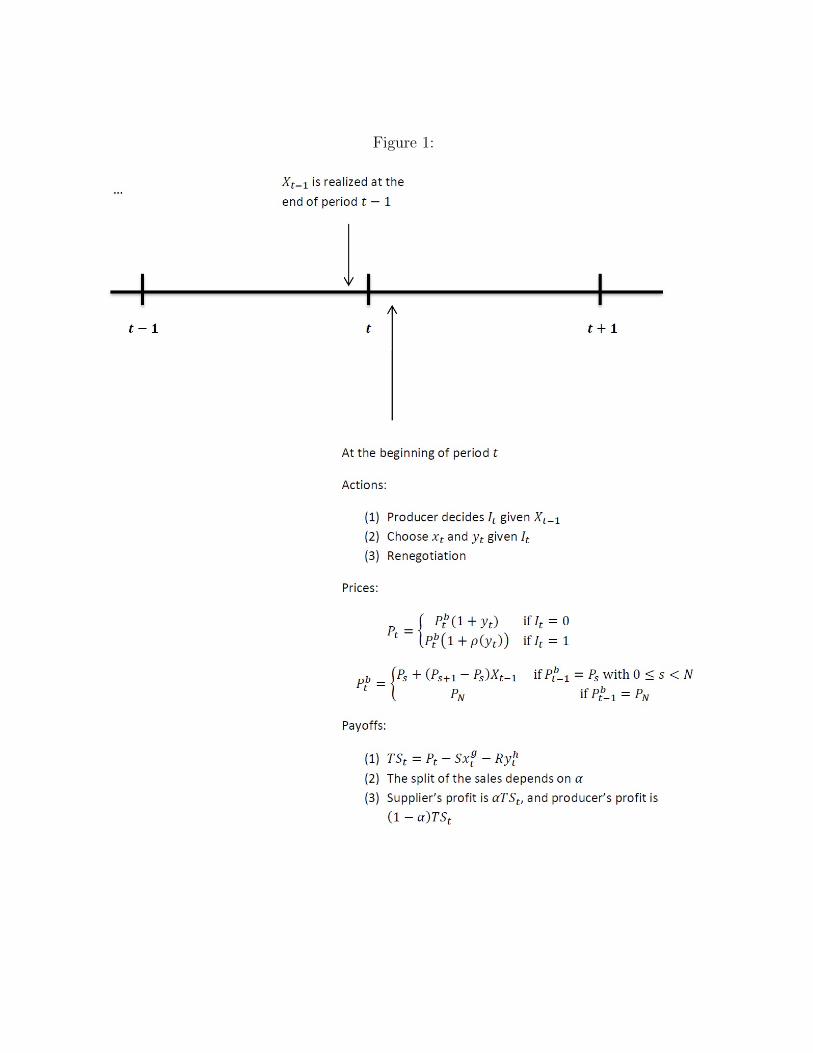
Figure 1:

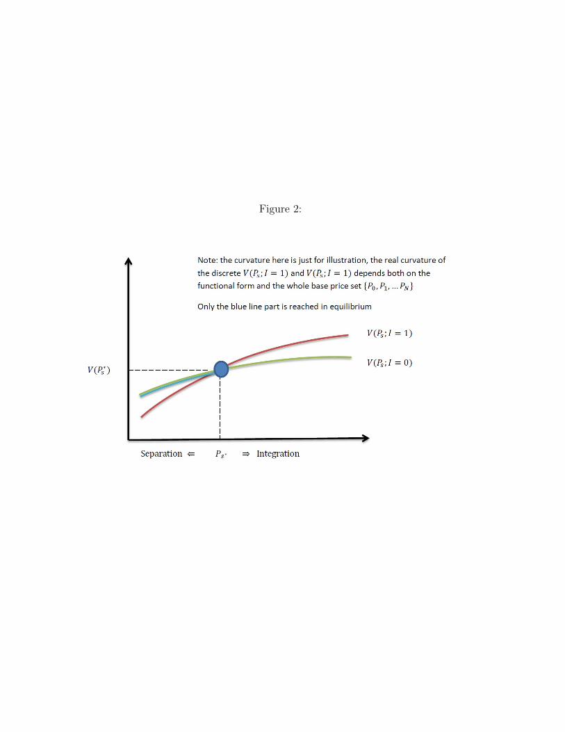
Figure 2:

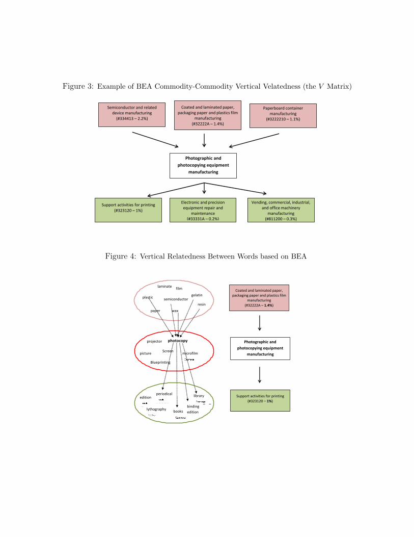
Figure 3: Example of BEA Commodity-Commodity Vertical Velatedness (the V Matrix)

Photographic andphotocopying equipment

manufacturing

Semiconductor and relateddevice manufacturing

(#334413 2.2%)

Coated and laminated paper,packaging paper and plastics film

manufacturing(#32222A 1.4%)

Paperboard containermanufacturing

(#3222210 1.1%)

Support activities for printing(#323120 1%)

Electronic and precisionequipment repair and

maintenance(#33331A 0.2%)

Vending, commercial, industrial,and office machinery

manufacturing(#811200 0.3%)

Figure 4: Vertical Relatedness Between Words based on BEA

photocopy

Screenpicture

Blueprinting

microfilm

projector

plastic semiconductorresin

waxpaper

gelatin

filmlaminate

library

books

edition

bindingedition

periodical

lythography

Coated and laminated paper,packaging paper and plastics film

manufacturing(#32222A 1.4%)

Photographic andphotocopying equipment

manufacturing

Support activities for printing(#323120 1%)

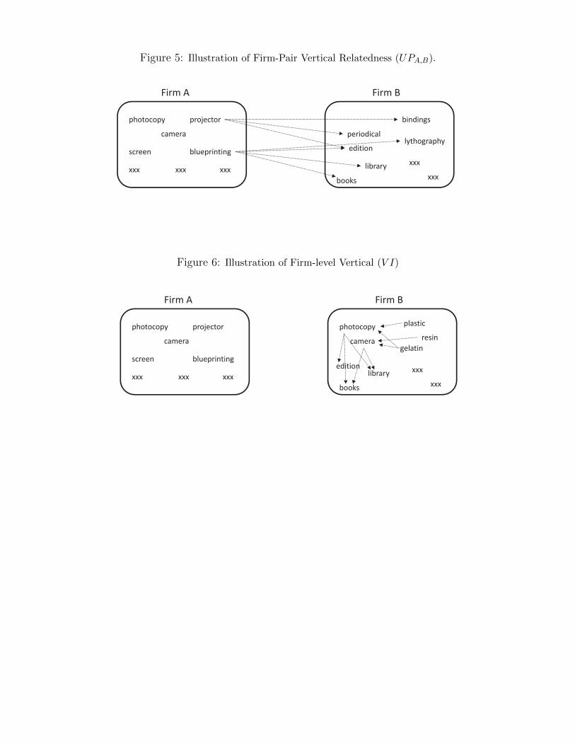
Figure 5: Illustration of Firm-Pair Vertical Relatedness (UPA,B).

Firm A Firm B

photocopy projector

camera

screen blueprinting

xxx xxx xxx

bindings

periodical

editionlythography

library

books

xxx

xxx

Figure 6: Illustration of Firm-level Vertical (V I)

Firm A Firm B

photocopy projector

camera

screen blueprinting

xxx xxx xxx

photocopy

camera

edition

gelatin

library

books

xxx

xxx

plastic

resin

Figure 7: R&D and Patents prior to acquisitions. The figure shows the average R&D (lowerpanel) and patenting activity (upper panel) of firms that are targets in vertical and non-verticalacquisitions prior to the acquisition. Solid lines represent vertical transactions identified usingthe Vertical Text-10% network. Dashed lines represent non-vertical transactions.

.45

.5.5

5.6

.65

.7lo

g(#p

aten

ts)

-3 -2 -1 0Years prior to acquisition

.008

.008

5.0

09.0

095

#pat

ents

/ass

ets

-3 -2 -1 0Years prior to acquisition

.04

.06

.08

.1.1

2R

&D

/sal

es

-3 -2 -1 0Years prior to acquisition

Figure 8: R&D intensity around vertical acquisitions. The figure shows the average R&D/salesaround the years that surround vertical transactions. The solid line displays all vertical targetsthat continue to exist for at least one year after being acquired. The dashed line displays“combined” entities that aggregate R&D and sales of acquirers and targets. Vertical transactionsare identified using the Vertical Text-10% network.

.02

.04

.06

R&

D/s

ales

-3 -2 -1 0 1 2 3Years around acquisition

Target Combined Entity

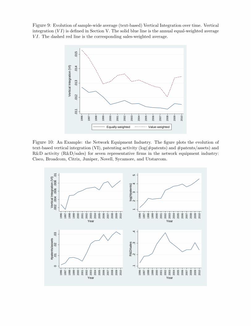
Figure 9: Evolution of sample-wide average (text-based) Vertical Integration over time. Verticalintegration (V I) is defined in Section V. The solid blue line is the annual equal-weighted averageV I. The dashed red line is the corresponding sales-weighted average.

.011

.012

.013

.014

.015

Ver

tical

Inte

grat

ion

(VI)

1996

1997

1998

1999

2000

2001

2002

2003

2004

2005

2006

2007

2008

2009

2010

Equally-weighted Value-weighted

Figure 10: An Example: the Network Equipment Industry. The figure plots the evolution oftext-based vertical integration (VI), patenting activity (log(#patents) and #patents/assets) andR&D activity (R&D/sales) for seven representative firms in the network equipment industry:Cisco, Broadcom, Citrix, Juniper, Novell, Sycamore, and Utstarcom.

.002

.004

.006

.008

.01

Ver

tical

Inte

grat

ion

(VI)

1996

1997

1998

1999

2000

2001

2002

2003

2004

2005

2006

2007

2008

2009

2010

Year

12

34

5lo

g(#p

aten

ts)

1996

1997

1998

1999

2000

2001

2002

2003

2004

2005

2006

2007

2008

2009

2010

Year

0.0

1.0

2.0

3#p

aten

ts/a

sset

s

1996

1997

1998

1999

2000

2001

2002

2003

2004

2005

2006

2007

2008

2009

2010

Year

.1.2

.3.4

R&

D/s

ales

1996

1997

1998

1999

2000

2001

2002

2003

2004

2005

2006

2007

2008

2009

2010

Year