using source-to-source transformations to add debug
TRANSCRIPT

Brigham Young University Brigham Young University
BYU ScholarsArchive BYU ScholarsArchive
Theses and Dissertations
2016-03-01
Using Source-to-Source Transformations to Add Debug Using Source-to-Source Transformations to Add Debug
Observability to HLS-Synthesized Circuits Observability to HLS-Synthesized Circuits
Joshua Scott Monson Brigham Young University - Provo
Follow this and additional works at: https://scholarsarchive.byu.edu/etd
Part of the Electrical and Computer Engineering Commons
BYU ScholarsArchive Citation BYU ScholarsArchive Citation Monson, Joshua Scott, "Using Source-to-Source Transformations to Add Debug Observability to HLS-Synthesized Circuits" (2016). Theses and Dissertations. 5871. https://scholarsarchive.byu.edu/etd/5871
This Dissertation is brought to you for free and open access by BYU ScholarsArchive. It has been accepted for inclusion in Theses and Dissertations by an authorized administrator of BYU ScholarsArchive. For more information, please contact [email protected], [email protected].

Using Source-to-Source Transformations to Add Debug Observability
to HLS-Synthesized Circuits
Joshua Scott Monson
A dissertation submitted to the faculty ofBrigham Young University
in partial fulfillment of the requirements for the degree of
Doctor of Philosophy
Brad L. Hutchings, ChairBrent NelsonDoran Wilde
Michael J. WirthlinDavid Penry
Department of Electical and Computer Engineering
Brigham Young University
March 2016
Copyright © 2016 Joshua Scott Monson
All Rights Reserved

ABSTRACT
Using Source-to-Source Transformations to Add Debug Observabilityto HLS-Synthesized Circuits
Joshua Scott MonsonDepartment of Electical and Computer Engineering, BYU
Doctor of Philosophy
This dissertation introduces a novel approach for exposing the internal, source-level ex-pressions of circuits generated by high-level synthesis (HLS) for in-circuit debug. The approachuses source-to-source transformations to instrument specific source-level expressions with debugports. These debug ports allow a user to connect a debugging instrument (e.g. an embedded logicanalyzer) to record the activity of the expression corresponding to the debug port. This dissertationdemonstrates that a debugging solution based on these source-to-source transformations is feasi-ble and that individual debug ports can be added for a cost of a 1-2% increase in circuit area onaverage. It also introduces another transformation that permits pointer-valued expressions to beinstrumented for debug. It is demonstrated that all pointers in the CHStone benchmarks can beinstrumented for an average 4% increase in circuit area.
The debug port transformations are demonstrated on two HLS tools – Vivado HLS andLegup. The architecture of the source-to-source compiler allowed the necessary adaptations for thesecond tool (Legup) to be implemented using a minimal amount of additional code. Due to limita-tions in the Legup compiler an additional optimization was added to reduce the latency overheadincurred by the debug ports. User manuals and other documentation from 10 additional C-basedHLS tools is examined to determine whether they are amenable to debug instrumentation using thesource-to-source transformations. Of the 10 additional HLS tools examined, 6 were amenable tothe transformations, 3 were likely to be amenable, and 1 was not. This dissertation estimates thecost of a complete debugging solution (i.e. one with debug ports and a debugging instrument) andidentifies a possible worst case bound for adding debug ports. Finally, this dissertation analyzestwo different debugging instruments and determines which instrument would be best for most HLScircuit mapped to FPGAs. It then estimates the overhead of this debugging solution.
Keywords: FPGA, high-level synthesis, debugging, source-to-source transformations, embeddedlogic analyzer

ACKNOWLEDGMENTS
I would like to acknowledge and profoundly thank a number of people, without whose
support, I could not have completed this manuscript or the research that supports it. First and
foremost, I must thank Renae, my wife, for her support, patience, and encouragement throughout
the entirety of my PhD. I would also like to thank my children Lillian, Bruce, Ezra, and Reed
for their support and love. I would like to address special thanks to my daughter Lillian who has
patiently shared her closet-less bedroom with her younger brothers during the many years of my
graduate work. During the difficult times of my PhD, that is, those times when I wondered if I was
intelligent or capable enough to complete this degree, it was always nice to come home and know
that I had the support and love of my family whether I was successful or not.
I must also extend my thanks and gratitude to my parents, Scott and Debbie Monson, for
their love, support, and for teaching me the gospel of Jesus Christ. The faith that I learned in
my home (growing up) has helped sustain me through the difficult portions of this degree. I must
also thank my extended family (on both the Monson and Ives sides) for their advice and words of
encouragement over the last several years.
I also owe a great debt of gratitude to my adviser, Brad Hutchings, whose patient mentoring
and professional example was instrumental to the completion of this document and will guide me
during the remainder of my career. In addition, I need to express my gratitude to the faculty of
the BYU Electrical and Computer Engineering Department, especially Brent Nelson and Mike
Wirthlin, for developing and maintaining an excellent engineering program from which I have
learned so much. I would also like to thank my good friends Travis Haroldsen and Jon-Paul
Anderson for their friendship and support. I would also like to express my gratitude to Chris Lavin
who answered my endless questions about pursuing a PhD and set an excellent example of how to
pursue it.
Finally, I would like to express my eternal gratitude to my Savior and my Heavenly Father
for blessing me with this opportunity and then providing the strength and support to complete it.

TABLE OF CONTENTS
LIST OF TABLES . . . . . . . . . . . . . . . . . . . . . . . . . . . . . . . . . . . . . . . vii
LIST OF FIGURES . . . . . . . . . . . . . . . . . . . . . . . . . . . . . . . . . . . . . . viii
LIST OF LISTINGS . . . . . . . . . . . . . . . . . . . . . . . . . . . . . . . . . . . . . . ix
Preface . . . . . . . . . . . . . . . . . . . . . . . . . . . . . . . . . . . . . . . . . . . . . x
Chapter 1 Introduction . . . . . . . . . . . . . . . . . . . . . . . . . . . . . . . . . . . 11.1 Motivation . . . . . . . . . . . . . . . . . . . . . . . . . . . . . . . . . . . . . . . 11.2 Summary of Research . . . . . . . . . . . . . . . . . . . . . . . . . . . . . . . . . 31.3 Research Contributions . . . . . . . . . . . . . . . . . . . . . . . . . . . . . . . . 51.4 Potential Applications . . . . . . . . . . . . . . . . . . . . . . . . . . . . . . . . . 61.5 Dissertation Organization . . . . . . . . . . . . . . . . . . . . . . . . . . . . . . . 7
Chapter 2 Background and Related Work . . . . . . . . . . . . . . . . . . . . . . . . 82.1 FPGA Architecture and Development . . . . . . . . . . . . . . . . . . . . . . . . 8
2.1.1 FPGA Architecture . . . . . . . . . . . . . . . . . . . . . . . . . . . . . . 92.1.2 Register Transfer Level Design . . . . . . . . . . . . . . . . . . . . . . . . 112.1.3 Application Development on FPGAs . . . . . . . . . . . . . . . . . . . . 11
2.2 HLS Tool Flow and Development . . . . . . . . . . . . . . . . . . . . . . . . . . 132.2.1 Parsing/Compiler Optimizations . . . . . . . . . . . . . . . . . . . . . . . 142.2.2 Scheduling . . . . . . . . . . . . . . . . . . . . . . . . . . . . . . . . . . 142.2.3 Binding . . . . . . . . . . . . . . . . . . . . . . . . . . . . . . . . . . . . 152.2.4 RTL Generation . . . . . . . . . . . . . . . . . . . . . . . . . . . . . . . 152.2.5 HLS Application Development . . . . . . . . . . . . . . . . . . . . . . . . 15
2.3 Debugging Approaches on FPGAs . . . . . . . . . . . . . . . . . . . . . . . . . . 162.3.1 Trace-Based Debugging Approaches . . . . . . . . . . . . . . . . . . . . . 17
2.4 Current Approaches for Debugging High-Level Synthesis . . . . . . . . . . . . . . 182.4.1 Previous Work: Adding Debug Prior To High-Level Synthesis . . . . . . . 192.4.2 Previous Work: Adding Debug Support into The HLS tool . . . . . . . . . 202.4.3 Previous Work: Adding Debug After High-Level Synthesis . . . . . . . . . 212.4.4 Previous Work: Source-To-Source Compilation and High-Level Synthesis . 22
2.5 Source-to-Source Transformations . . . . . . . . . . . . . . . . . . . . . . . . . . 222.5.1 Source-to-Source Compilation . . . . . . . . . . . . . . . . . . . . . . . . 232.5.2 Intermediate Representation . . . . . . . . . . . . . . . . . . . . . . . . . 232.5.3 Modifying the AST . . . . . . . . . . . . . . . . . . . . . . . . . . . . . . 24
2.6 Conclusion . . . . . . . . . . . . . . . . . . . . . . . . . . . . . . . . . . . . . . 24
Chapter 3 Debug Port Transformation and Feasibility . . . . . . . . . . . . . . . . . 253.1 Instrumenting Expressions for Debug In Vivado HLS . . . . . . . . . . . . . . . . 26
3.1.1 Instrumenting an Expression . . . . . . . . . . . . . . . . . . . . . . . . . 27
iv

3.1.2 Implementation in a Source-to-Source Compiler . . . . . . . . . . . . . . 293.1.3 Using the Source-to-Source Compiler . . . . . . . . . . . . . . . . . . . . 30
3.2 Feasibility of the Debug Port Transformation . . . . . . . . . . . . . . . . . . . . 303.2.1 Feasibility Experiments . . . . . . . . . . . . . . . . . . . . . . . . . . . 323.2.2 Single-Port Experiments . . . . . . . . . . . . . . . . . . . . . . . . . . . 363.2.3 Multi-Port Experiments . . . . . . . . . . . . . . . . . . . . . . . . . . . 47
3.3 Conclusion . . . . . . . . . . . . . . . . . . . . . . . . . . . . . . . . . . . . . . 52
Chapter 4 Instrumenting Pointers In Vivado HLS . . . . . . . . . . . . . . . . . . . . 544.1 Shadow Pointer Transformation . . . . . . . . . . . . . . . . . . . . . . . . . . . 55
4.1.1 Shadow Pointers . . . . . . . . . . . . . . . . . . . . . . . . . . . . . . . 554.1.2 Shadow Pointer Insertion . . . . . . . . . . . . . . . . . . . . . . . . . . . 584.1.3 Current Limitations of Shadow Pointers . . . . . . . . . . . . . . . . . . . 60
4.2 Experiments . . . . . . . . . . . . . . . . . . . . . . . . . . . . . . . . . . . . . . 604.2.1 Results . . . . . . . . . . . . . . . . . . . . . . . . . . . . . . . . . . . . 614.2.2 Optimization Effects . . . . . . . . . . . . . . . . . . . . . . . . . . . . . 624.2.3 Any Room For Improvement? . . . . . . . . . . . . . . . . . . . . . . . . 64
4.3 Conclusion . . . . . . . . . . . . . . . . . . . . . . . . . . . . . . . . . . . . . . 64
Chapter 5 Migrating Transformations to LegUp . . . . . . . . . . . . . . . . . . . . . 665.1 Primary Differences between Vivado HLS and LegUp . . . . . . . . . . . . . . . . 66
5.1.1 LegUp . . . . . . . . . . . . . . . . . . . . . . . . . . . . . . . . . . . . 665.1.2 Xilinx Vivado HLS . . . . . . . . . . . . . . . . . . . . . . . . . . . . . . 68
5.2 Source-to-Source Compiler Architecture . . . . . . . . . . . . . . . . . . . . . . . 685.3 Migrating Transformations to LegUp . . . . . . . . . . . . . . . . . . . . . . . . . 69
5.3.1 Using Custom Verilog Modules to Implement Debug Ports in LegUp . . . 715.3.2 Compiler Modifications to Support LegUp . . . . . . . . . . . . . . . . . 75
5.4 Improvements to Port-Binding Strategy . . . . . . . . . . . . . . . . . . . . . . . 755.4.1 Naive/Default Binding Approach . . . . . . . . . . . . . . . . . . . . . . 765.4.2 Delayed Port-Binding Strategy . . . . . . . . . . . . . . . . . . . . . . . . 765.4.3 Delayed Binding Algorithm . . . . . . . . . . . . . . . . . . . . . . . . . 785.4.4 Debugging Deadlock using the Delayed Binding Approach . . . . . . . . . 82
5.5 Experiments and Results . . . . . . . . . . . . . . . . . . . . . . . . . . . . . . . 835.5.1 Experiments . . . . . . . . . . . . . . . . . . . . . . . . . . . . . . . . . 835.5.2 Results . . . . . . . . . . . . . . . . . . . . . . . . . . . . . . . . . . . . 845.5.3 Effect of Delayed-Binding Strategy . . . . . . . . . . . . . . . . . . . . . 845.5.4 Latency Overhead . . . . . . . . . . . . . . . . . . . . . . . . . . . . . . 855.5.5 Cost of Individual Debug Ports . . . . . . . . . . . . . . . . . . . . . . . . 885.5.6 Comparison of LegUp and Vivado Results . . . . . . . . . . . . . . . . . . 895.5.7 Impact of Instrumenting Pointers . . . . . . . . . . . . . . . . . . . . . . . 905.5.8 Usability and Feasibility . . . . . . . . . . . . . . . . . . . . . . . . . . . 91
5.6 Conclusion . . . . . . . . . . . . . . . . . . . . . . . . . . . . . . . . . . . . . . 92
Chapter 6 Migrating Transformations to Other HLS Tools . . . . . . . . . . . . . . . 936.1 Disparities between Vivado HLS and LegUp Results . . . . . . . . . . . . . . . . 93
v

6.2 Required HLS tool Support for Source-to-Source Transformations . . . . . . . . . 946.3 Potential HLS Tool Candidates for Source-to-Source Transformations . . . . . . . 95
6.3.1 Tool-by-Tool Analysis . . . . . . . . . . . . . . . . . . . . . . . . . . . . 966.3.2 Analysis Summary and Discussion . . . . . . . . . . . . . . . . . . . . . . 99
6.4 Conclusion . . . . . . . . . . . . . . . . . . . . . . . . . . . . . . . . . . . . . . 100
Chapter 7 Bounds and Limits . . . . . . . . . . . . . . . . . . . . . . . . . . . . . . . 1027.1 Inserting Debug Ports at Minimum Cost . . . . . . . . . . . . . . . . . . . . . . . 102
7.1.1 Potential Effects if Conditions Are Not Met . . . . . . . . . . . . . . . . . 1037.2 Worst Case Overhead of Debug Port Transformation . . . . . . . . . . . . . . . . 104
7.2.1 Identifying a Worst-Case Bound . . . . . . . . . . . . . . . . . . . . . . . 1047.2.2 Experiment . . . . . . . . . . . . . . . . . . . . . . . . . . . . . . . . . . 1057.2.3 Results . . . . . . . . . . . . . . . . . . . . . . . . . . . . . . . . . . . . 1067.2.4 Common Optimizations Significantly Affected by Debug Ports . . . . . . . 107
7.3 Debugging Instrument Bound . . . . . . . . . . . . . . . . . . . . . . . . . . . . . 1087.3.1 Goeders’ Debugging Instrument . . . . . . . . . . . . . . . . . . . . . . . 1087.3.2 Keeley’s Debugging Instrument . . . . . . . . . . . . . . . . . . . . . . . 1097.3.3 Compare and Contrast the Debugging Instruments . . . . . . . . . . . . . 1097.3.4 Debugging Instrument and Complete Solution Overhead . . . . . . . . . . 111
7.4 Conclusion . . . . . . . . . . . . . . . . . . . . . . . . . . . . . . . . . . . . . . 113
Chapter 8 Conclusion and Future Work . . . . . . . . . . . . . . . . . . . . . . . . . 1148.1 Summary of Contributions . . . . . . . . . . . . . . . . . . . . . . . . . . . . . . 1148.2 Future Work . . . . . . . . . . . . . . . . . . . . . . . . . . . . . . . . . . . . . . 1158.3 Concluding Remarks . . . . . . . . . . . . . . . . . . . . . . . . . . . . . . . . . 117
REFERENCES . . . . . . . . . . . . . . . . . . . . . . . . . . . . . . . . . . . . . . . . . 119
Appendix A Estimating the Size of Goeders’ Debugging Instrument . . . . . . . . . . . 126A.1 Goeders and Wilton Implementation Data . . . . . . . . . . . . . . . . . . . . . . 126A.2 Structure of Goeders’ Debugging Instrument . . . . . . . . . . . . . . . . . . . . . 128A.3 Adaption for Use With Debug Port Transformation With Vivado HLS . . . . . . . 128A.4 Debugging Instrument Estimates . . . . . . . . . . . . . . . . . . . . . . . . . . . 129A.5 Results and Analysis . . . . . . . . . . . . . . . . . . . . . . . . . . . . . . . . . 129A.6 Comparison to LegUp Built-in Debug Support . . . . . . . . . . . . . . . . . . . . 130
vi

LIST OF TABLES
3.1 Area and Clock Constraints of Baseline Circuits . . . . . . . . . . . . . . . . . . . 353.2 Single Port Experiment Results . . . . . . . . . . . . . . . . . . . . . . . . . . . . 393.3 Effect of Single Port Experiments on Performance and Area . . . . . . . . . . . . 43
4.1 Experimental Results . . . . . . . . . . . . . . . . . . . . . . . . . . . . . . . . . 62
5.1 Simulation Latency Overhead . . . . . . . . . . . . . . . . . . . . . . . . . . . . 855.2 Area Overhead (LEs) . . . . . . . . . . . . . . . . . . . . . . . . . . . . . . . . . 855.3 Latency Impact of Single Ports . . . . . . . . . . . . . . . . . . . . . . . . . . . . 895.4 Area Impact of Single Ports . . . . . . . . . . . . . . . . . . . . . . . . . . . . . . 89
6.1 Summary of HLS Tool Analysis . . . . . . . . . . . . . . . . . . . . . . . . . . . 100
7.1 Experimental Results Compared to Unoptimized LegUp Results . . . . . . . . . . 1067.2 Debugging Instrument Overhead Estimates . . . . . . . . . . . . . . . . . . . . . 112
A.1 Debugging Instrument Overhead Estimates . . . . . . . . . . . . . . . . . . . . . 130
vii
LIST OF FIGURES
2.1 Example fixed width figure . . . . . . . . . . . . . . . . . . . . . . . . . . . . . . 102.2 Debugging Instrument In FPGA . . . . . . . . . . . . . . . . . . . . . . . . . . . 112.3 Standard FPGA Development Flow . . . . . . . . . . . . . . . . . . . . . . . . . 122.4 Block diagram of the typical HLS tool flow. . . . . . . . . . . . . . . . . . . . . . 132.5 Debugging Instrument In FPGA . . . . . . . . . . . . . . . . . . . . . . . . . . . 17
3.1 Debug Ports allow Developers to connect a debugging instrument to source-levelexpressions. . . . . . . . . . . . . . . . . . . . . . . . . . . . . . . . . . . . . . . 26
3.2 Inserting a debug port into the AST. . . . . . . . . . . . . . . . . . . . . . . . . . 283.3 The structure of a Rose-based source-to-source compiler. . . . . . . . . . . . . . . 293.4 The implementation flow used for each experiment. . . . . . . . . . . . . . . . . . 333.5 Distribution of LUT impact in dfmul benchmark. . . . . . . . . . . . . . . . . . . 383.6 Hard Clock Constraint Shifts Mean . . . . . . . . . . . . . . . . . . . . . . . . . . 423.7 Block diagram of multiplexer sharing a debug port. . . . . . . . . . . . . . . . . . 453.8 Multi-Port Experiment Results . . . . . . . . . . . . . . . . . . . . . . . . . . . . 493.8 (continued) Multi-Port Experiment Results . . . . . . . . . . . . . . . . . . . . . . 503.8 (continued) Multi-Port Experiment Results . . . . . . . . . . . . . . . . . . . . . . 51
4.1 Example of Connecting the Shadow Pointer Data Path to an ELA. . . . . . . . . . 63
5.1 Architecture of the source-to-source compiler. . . . . . . . . . . . . . . . . . . . . 695.2 Structure of Legup Accelerator RTL. . . . . . . . . . . . . . . . . . . . . . . . . . 725.3 Experimental Flow for Legup and Vivado HLS designs. . . . . . . . . . . . . . . . 835.4 Distribution of Latency Overhead . . . . . . . . . . . . . . . . . . . . . . . . . . 87
A.1 Growth of Goeders and Wilton’s ELA circuit with respect to bits traced. . . . . . . 127
viii

LIST OF LISTINGS
3.1 Instrumentation Example . . . . . . . . . . . . . . . . . . . . . . . . . . . . . . . 274.1 Shadow Pointer Examples . . . . . . . . . . . . . . . . . . . . . . . . . . . . . . 565.1 Examples of Vivado HLS and LegUp Transformations . . . . . . . . . . . . . . . 705.2 Custom Verilog Module for Debug Port Function in Listing 5.1 . . . . . . . . . . . 735.3 Example of Code Instrumented Using Default Binding Strategy . . . . . . . . . . . 775.4 Simple Example of Delayed Binding Approach . . . . . . . . . . . . . . . . . . . 795.5 Complex Example of Delayed Binding Approach . . . . . . . . . . . . . . . . . . 80
ix
PREFACE
Many of the research contributions presented in this thesis were previously published in
conference paper format. Specifically, the work of three published conference papers [1] [2] [3] are
included in this format. However, the discussions of methods, results, and research contributions
have been significantly expanded beyond that which was possible when the research was presented
in conference paper format. In general, the research contributions from each of these conference
papers are included and expanded upon in various chapters of this dissertation. For example,
Chapter 3 expands upon the research contributions in the FPGA [1] and FPT [2] papers. Both of
these papers discussed and tested the initial feasibility of the debug port transformation presented in
this dissertation. Chapter 4 presents the work shadow pointers that was presented in [3]. Chapter 5
discusses how the source-to-source compiler presented in this dissertation was modified to support
the LegUp high-level synthesis tool.
x

CHAPTER 1. INTRODUCTION
1.1 Motivation
Field programmable gate arrays (FPGA) are a common alternative to ASICs for imple-
menting circuits with high-performance and/or low-power requirements. In general, FPGAs are
often used instead of ASICs, because they provide lower non-recurring engineering (NRE) costs
and shorter time-to-market. These qualities make FPGAs ideal for use in low or medium vol-
ume products such as satellites [4], unmanned aerial vehicles (UAVs) [5], logic emulators, Internet
routers, and (most recently) data centers [6]. FPGAs are also commonly chosen over other general
computing platforms (e.g. GPUs, multi-core CPUs) because they often deliver higher performance
while consuming less power.
Despite their performance and power benefits, FPGAs are not always chosen to implement
high-performance applications. In general, FPGAs are passed by for two reasons. First, relative to
other general purpose computing platforms, FPGAs are difficult to program and have long compi-
lation and simulation times. These factors become deterrents to FPGA use in projects with short
deadlines and/or when easier-to-program computing platforms provide sufficient performance and
sufficiently low power consumption. Second, the use of an FPGA may not even be considered
because a developer with the required hardware expertise is not available.
To address the challenges of FPGA development, increasing numbers of developers are
turning to High-Level Synthesis tools (HLS). In general, an HLS tool is any compiler that is able
to generate RTL code (which can be mapped to an FPGA) from a specification written in a standard
programming language (e.g. C, C++, Java, Matlab). The use of high-level languages allows HLS
users to develop, debug, and verify applications on a desktop PC while leveraging mature, industry-
standard software development tools and environments before passing their code to an HLS tool
for synthesis. Because the application is first developed and debugged in software, HLS users
are often able to avoid the long simulation times associated with developing and debugging an
1

application written in an RTL language. In fact, the use of HLS tools has been shown, in certain
instances, to reduce development time by 5X while producing circuits comparable to hand-written
RTL [7].
Even though most of the validation and debugging of an HLS-generated circuit is per-
formed quickly in software, there is still a potential for difficult-to-find bugs to appear after the
design has been placed in an FPGA and exposed to real-world data. These types of bugs can
arise from system-level interactions with the surrounding environment (e.g. I/O devices) or other
modules in the system [8]. Further, the complexity of some system environments can make it
impossible to thoroughly test the HLS IP in software or in RTL simulation [8]. There is also the
possibility of errors in the HLS tool although these may be better handled by automated discrep-
ancy detection approaches [9] [10] [11]. Finding the root cause of these bugs is especially difficult
because real-world environments do not make it easy for the user to observe the execution of the
circuit.
The behavior of a circuit executing on an FPGA can be observed by instrumenting the
circuit with a debugging instrument known as an embedded logic analyzer (ELA). In order to use
an ELA, the user is required to identify a set of signals-of-interest that will help him isolate the bug.
These signals are connected to a memory bank (via intermediate signals or probes) in the ELA that
keeps a history of the values of the signal-of-interest. When the buggy behavior is encountered the
history leading up to that bug is locked into the memory bank and uploaded to the users workstation
for analysis.
The process of instrumenting an HLS design with an ELA is complicated by the fact that
it is difficult for the user to identify useful signals (i.e. those that correspond to source-level ex-
pressions that the user understands) to record with the ELA. This problem is compounded by the
fact that current commercial HLS tools do not automate the process in any way. Therefore, when
a bug manifests during in-circuit operation, the user must perform the whole task of setting up the
debugging instrument on his own. This can be a daunting and time-consuming task for at least
two reasons. First, in the best case, the general HLS-user is a hardware engineer who is merely
unfamiliar with newly generated HLS RTL and will need to invest time into understanding how it
is structured. In the worst case, the HLS-user is a software programmer who will not understand
the structure of the generated RTL. Second, in order to “connect” specific source-level variables
2

or expressions to the debugging instrument the HLS-user must identify all RTL signals that corre-
spond to the variable or expression (may be duplicated in hardware). For these RTL signals to be
useful, the HLS-user must also be able to identify when they are valid and when they correspond to
the source-level variable of interest (i.e. due to resource sharing the RTL signals may correspond
to different source-level variables or expressions at different points in execution; further there may
be points where an RTL signals has no correspondence at all). This means that the user is also
required to identify and connect to the debugging instrument all RTL expressions and signals that
validate the data and correspondence (state machines signals, process if-statement conditionals,
etc.). It is true that at least one commercial HLS tool (i.e. Vivado HLS [12]) provides some infor-
mation about the correspondence between the original source code and the generated RTL code;
however, it is the author’s experience that the provided information is not sufficient for a general
debugging solution.
1.2 Summary of Research
The primary focus of this dissertation is to introduce source-to-source transformations that
simplify the process of instrumenting an HLS-generated IP core for debug (i.e. connecting it to a
debugging instrument) and demonstrate that these transformations are feasible for use in real-world
debugging scenarios. This is accomplished by first introducing a source-to-source transformations
(hereafter known as the debug port transformation) that can be automatically applied to direct the
HLS tool to add debug ports into the RTL code of HLS-generated IP cores. Each of these debug
ports corresponds to and is wired directly to the result of a specific source-level expression and can
be easily connected to a debugging instrument via a simple data-valid interface. In this way, the
debug port transformation relieves the HLS-user of the error-prone process involved in properly
identifying the signals that correspond to the source-level expressions that he/she would like to
observe with the debugging instrument.
Despite the many benefits of the debug port transformation, it also has the potential to
increase the size and reduce the performance of the circuit to which it is applied. In most cases,
the only extra circuitry added by the HLS tool to implement the debug port is a wire and a small
amount of logic to implement a data valid signal. However, it has been observed that instrumenting
a single expression with a debug port can alter the way in which a circuit is optimized as well as
3

change its structure. Both of these changes can increase the size and reduce the performance of
the debug-port instrumented circuit potentially to the point where the debug port instrumentation
approach is no longer feasible.
To demonstrate that the debug port transformation is indeed a feasible means to expose
the internal expressions of an HLS-generated IP core to a debugging instrument this dissertation
examines the results of two large sets of experiments. These experiments reveal that the debug port
transformation can have a wide range of effects on a circuit whether it is used to instrument one
expression or a large group of expressions. For example, these experiments revealed that when a
single expression is instrumented it can actually improve both the area and performance of the cir-
cuit or it can significantly degrade both. In another example, the first 33 expressions instrumented
with debug ports (in a special order) reduced the area of the circuit; however, instrumenting the
remaining 50 expressions increased the area by almost 30%. These experiments were run in the
Vivado HLS tool.
Once feasibility is established for Vivado HLS, the debug port transformation is migrated
to a second HLS tool – LegUp [13]. Migrating the debug port transformation to LegUp merely
required the creation of a small component that applied the LegUp-specific syntax for creating a
port. However, the initial approach in LegUp – a direct mapping of the Vivado HLS approach
– resulted in an unacceptable amount of latency overhead when hundreds of signals were instru-
mented. An alternative binding strategy that groups multiple expressions to a single debug port is
proposed and used to mitigate the excessive latency overhead. A subset of more realistic scenarios
that instrument a single debug port are examined and shown to result in much lower overhead. A
comparison is then made between the LegUp and Vivado HLS results.
This dissertation also identifies that pointer values (addresses) in both Vivado HLS and
LegUp cannot be written to debug ports. A transformation is proposed that inserts integer vari-
ables, called shadow pointers, to convey an equivalent form of the addresses held by pointers to the
debug ports. This transformation is shown to work in both Vivado HLS and LegUp and results in a
relatively small amount of overhead and required no changes to the source code that implemented
the transformation.
This dissertation then examines the potential best and worst case bounds associated with
using the debug port and shadow pointer transformations. It also uses data from the dissertation as
4

well as data from previously published papers to estimate the cost of a complete debugging solution
based on the transformations presented in this dissertation. This dissertation also identifies other
HLS tools that may be amenable to the proposed transformation and identifies potential future
work.
The key results of this dissertation are:
1. The debug port transformation is a feasible means for exposing source-level expressions to
a debugging instrument. This is demonstrated by the fact our experiments revealed that 90-
99% of expressions (in the CHStone benchmarks) can be instrumented with debug ports for
an individual cost of a 1-6% increase in LUT count and on average all assignment operations
can be instrumented for an average 27% increase in LUT count.
2. The shadow pointer transformation can be used to expose the results of all pointer-valued
expressions to the debugging instrument for an average cost of 2.5% (over the CHStone
benchmarks). This result held even when all assignment operations were also instrumented
with debug ports.
3. The debug port transformation was demonstrated in a second HLS tool – LegUp. After
instrumentation the latency of the circuit increased by an average of 3.7X; however, the
delayed binding strategy proposed in this dissertation reduced the latency overhead to an
average of 1.95X.
4. Other than Vivado HLS and LegUp, documentation from 10 additional HLS tools were ex-
amined to determine how amenable they were to the debug port transformation. Of the 10
HLS tools examined, 6 were found to be amenable, 3 were likely to be amenable, and one
was not.
1.3 Research Contributions
The following is a list of the research contributions of this dissertation:
• A comprehensive review of HLS debugging approaches.
• A source-to-source transformation that instruments arbitrary expressions with debug ports.
The transformation ensures that the expression will exist in the final circuit.
5

• A transformation that allows pointer-valued expressions to be instrumented by the debug
port transformation.
• A large-scale experiment (utilizing over 50,000 individual place and route runs) that demon-
strates the feasibility of the source-to-source instrumentation approach.
• A demonstration that the source-to-source compiler can be extended to work with multiple
HLS tools.
• A novel debug-port binding approach that significantly deceases the latency overhead of de-
bug ports in HLS tools that have fixed latency overhead for I/O operations (such as LegUp).
• A survey of existing HLS tool documentation to determine other existing HLS tools that are
amenable to the debug port transformations.
• The determination of a reasonable upper bound for the overhead inflicted by the debug port
transformation.
• A comparison between a debug port transformation-based debugging solution and the built-
in debugging support for LegUp.
1.4 Potential Applications
The transformations presented in this dissertation could potentially be used as the founda-
tion of an automated debugging solution for an academic or commercial HLS tool. The benefit of
the source-to-source approach is that the HLS tool developers do not have to modify their tools
much – if at all – to support the transformations. Rather, they simply have to ensure that their tools
meet the criteria set forth in Section 6.2 of this dissertation.
Another potential application of this work would be to open-source the source-to-source
compiler presented in this dissertation. This would allow the users of Vivado HLS to more eas-
ily instrument their HLS-generated IP for in-system debug using both the transformations and a
commercial debugging instrument (e.g. SignalTap Chipscope). As discussed in Section 5.2, the
compiler is designed in a modular fashion and could easily be extended to support additional tools
and could be the basis of many interesting research projects.
6

1.5 Dissertation Organization
Chapter 2 discusses previous work and provides background information on various re-
lated topics.
Chapter 3 introduces the debug port transformation and reports on a feasibility study.
Chapter 4 introduces the shadow pointer transformation which allows pointer-valued ex-
pressions to be instrumented using the debug port transformation.
Chapter 5 demonstrates that the debug port transformations can be migrated to another
HLS tool (LegUp) and discusses a new binding approach that reduces latency overhead for LegUp
designs.
Chapter 6 determines that not all HLS tools are amenable to the source-to-source trans-
formation approach and identifies the features required to make them amenable. Several HLS
tools are then examined to determine whether or not they are amenable to the source-to-source
transformations.
Chapter 7 examines the best and worst case bounds of the debug port transformation. It
also examines two debugging instruments and determines which debugging instrument would be
the best fit for use in HLS circuits and then estimates the cost of this debugging instrument.
Chapter 8 provides a summary of the completed research and results. It also examines
several potential items for future work. It also provides some concluding remarks.
7

CHAPTER 2. BACKGROUND AND RELATED WORK
To motivate our discussion of current and past debugging practices on FPGAs, this chapter
describes FPGA architecture and standard RTL and C-based development flows. FPGA applica-
tion development using HLS is also described. This chapter also examines the various approaches
for performing on-chip debugging of FPGA-based applications. Previous research efforts applying
these debugging approaches to HLS are then described. This chapter also describes some foun-
dational concepts related to source-to-source transformations which are an important topic in this
dissertation.
2.1 FPGA Architecture and Development
Throughout their history, the key feature of FPGAs has always been its ability to be re-
configured to implement any simple or complex digital logic circuit which the FPGA has enough
resources to implement. When they where first introduced by Xilinx in 1989 [14], FPGAs were
primarily used to implement so-called “glue logic” between discrete components on printed circuit
boards (PCB) [15]. Examples of glue logic consist of simple logic functions (e.g. AND, OR, NOT)
and larger functions such as address decoders and state machines. The use of FPGAs to implement
glue logic allowed engineers to consolidate functions implemented by multiple discrete compo-
nents into a single device thereby decreasing the number of discrete components on the PCB.
However, as the capacity and performance of FPGAs has increased with Moore’s law, the role of
FPGAs has increased from simple glue logic to larger applications such as complex parallel com-
puting algorithms and systems-on-chip. As a example of the expanding role of FPGAs, Microsoft
recently announced its Catapult project [6] in which FPGAs were used to accelerate a portion of
the Bing ranking algorithm by almost 2X while only increasing power consumption by 10%. The
recent increases in the size and complexity of the applications mapped to FPGAs as well as the
desire of FPGA vendors to increase the FPGA user-base has forced FPGA vendors to improve
8

the design productivity of their tools [16] [17] [18]. These improvements include the adoption of
HLS tools (e.g. Vivado HLS, SDAccel) and graphical RTL design tools such as IP Integrator. The
remainder of this section discusses basic FPGA architecture and application development using
FPGA CAD tools in detail.
2.1.1 FPGA Architecture
As shown in Figure 2.1, an FPGA consists of a regular array of programmable logic blocks
and interconnect. This is known as an island-style architecture. The general idea is that the logic
blocks are ’floating’ in a sea of interconnect. The logic blocks are used to implement digital func-
tions while interconnect (switch-boxes) are used to create physical connections (wires) between
the inputs and outputs of the logic blocks. For example, Figure 2.2 shows a portion of the FPGA
being used to implement the AND gate. As shown in the figure, inputs A and B enter the FPGA
through the I/O logic blocks and are routed to the logic block that is programmed to implement
the AND gate. The result of the AND gate is then routed through several switch-boxes and finally
off-chip through another I/O block.
Generally speaking, FPGAs consist of two types of logic blocks: fine-grained and coarse-
grained. As shown in Figure 2.1, fine-grained logic blocks generally consist of several pairs of
look-up tables (LUT) and flip-flops (FF) as well as dedicated carry chain logic (not shown) to aid
in the efficient implementation of arithmetic units (e.g. adders, multipliers). LUTs are function
generators that can be used to implement arbitrary logic functions of n-inputs and (generally) one
output (where n is the number of inputs to the LUT). If a logic function is too large for a single LUT
(i.e. the function has more inputs or outputs than available on the LUT), the FPGA architecture is
flexible enough to allow multiple LUTs to be used together to implement the function. As shown
in Figure 2.1, FFs are placed adjacent to LUT outputs to allow the FF to register LUT outputs with
the least possible effect on the performance of the circuit.
As shown in Figure 2.1, FPGAs also contain coarse-grained logic blocks. Coarse-grained
logic blocks are fixed implementations of commonly-used digital functions that have been inte-
grated into the FPGA fabric. Since they implement fixed-functions, the underlying semi-conductor
layout of coarse-grained logic blocks is smaller and achieves higher performance and lower power
than an equivalent function implemented using fine-grained logic blocks. The most common ex-
9

SB
SB
SB
SB
SB
BRAM
SB
SB
DSP
SB
SB
SBSB SBI/OSB SB
SB
SBSB SBI/OSB I/OSB
SBSB SBI/OSB SERDESSB
SERDES
Figure 2.1: An example of an island-style FPGA architecture.
amples of digital functions implemented within coarse-grained logic blocks are on-chip memories
(BRAM) and multiply-accumulate units (DSP). The use of coarse-grained logic blocks also pro-
vides a means for FPGA architects to integrate functionality (into the FPGA) that cannot be imple-
mented using fined-grained logic blocks. Examples of these circuits include high-speed serial I/O
(SERDES), analog-to-digital converters, and temperature and power monitoring circuits.
10

SB
I/O
SB
SB
I/O
SBAB
C
Figure 2.2: An AND gate implemented on an FPGA. Inputs (A,B) and the output (C) are shown inred on the I/O blocks on the left.
2.1.2 Register Transfer Level Design
Designers currently specify most FPGA applications using Register Transfer Level (RTL)
languages. RTL design provides a relatively high abstraction level to perform detailed low-level
hardware design. Essentially, RTL languages allow hardware engineers to easily define how reg-
isters and other memory elements are updated on each clock cycle. Further, RTL languages like
Verilog and VHDL also allow hardware engineers to seamlessly switch between different design
abstraction levels (i.e. structural and behavioral). Thus RTL provides the engineer with a great
deal of control over the architecture of the design.
2.1.3 Application Development on FPGAs
As shown in Figure 2.3, the development of a working FPGA circuit from a set of appli-
cation requirements can be broken down into three phases: RTL development, running the vendor
tool flow, and on-chip execution. During RTL development, the developer codifies the application
requirements into an RTL specification (written in Verilog or VHDL). The developer then simu-
lates the RTL specification to determine whether the RTL specification meets the requirements. If
the RTL does not meet the requirements, the developer reviews the simulation to identify any errors
11

Vendor Tool FlowSynthesis
and Mapping
Placement & Routing
BitstreamGeneration
Application Requirements
On-Chip Execution
DownloadBitstream
In-Circuit Debugging
RTL Development
Write RTL
Simulate RTL
Debug
Working FPGA Application
Figure 2.3: This is the standard approach for RTL-based development on FPGAs.
in the specification (bugs) and makes appropriate adjustments to the RTL. This process, known as
debugging, is repeated until the RTL meets all of the application’s requirements. RTL simulation
is generally the best point in the development process to debug the functional specification of an
application because compilation times are relatively short and circuit visibility is high.
Once the developer has determined that the RTL specification is correct, the RTL is passed
to the FPGA vendor’s tool flow. In general, a vendor tool flow consists of three phases: logic
synthesis and technology mapping; placement and routing; and bitstream generation. These phases
translate the RTL specification into a gate-level netlist, efficiently map it to the FPGA, and generate
a configuration file (i.e. a bitstream). Rather than attempting to find the optimal mapping of
an RTL specification to the FPGA (which is a computationally infeasible problem) the vendor’s
CAD tools search the circuit design space for a mapping that will meet the application developer’s
requirements. Even though the vendor’s tools do not attempt to achieve the optimal circuit tool
12

Parsing and Compiler
OptimizationsScheduling Binding
RTL Generation
HLLSource File
RTL File
Figure 2.4: Block diagram of the typical HLS tool flow.
run-times can still be lengthy. For example, in commercial environments run-times of hours and
days are not uncommon [19].
The final step in the RTL development process is to download and execute the application
on the FPGA. This step is necessary to ensure that the design actually works on the device as
specified. Errors found during in-circuit execution are difficult to fix due to the speed of execution
and low observability of circuit signal values. This underscores the importance of catching as many
errors in simulation as possible.
2.2 HLS Tool Flow and Development
This section describes the fundamental concepts of HLS that form the foundation of much
of the discussion in this dissertation. The primary function of an HLS tool is to transform a circuit
specification described using a high-level language (HLL), such as C++ or Java, and output an
RTL design that can be mapped to an FPGA or ASIC circuit. Canonically speaking, this HLL-
to-RTL transformation is accomplished in three separate phases: 1) Scheduling, 2) Binding, and
3) RTL generation. In addition, HLS tools also leverage a compiler front end that provides a
parser and common compiler optimizations. Figure 2.4 is a block diagram that shows the most
common ordering of the HLS phases. Note, however, that the ordering shown in Figure 2.4 is
not strict and can be altered by the tool developer. For example, an HLS tool developer may find
that circuit quality increases if binding is performed prior to scheduling. The remainder of this
section discusses each of these phases in detail and ends with a discussion on FPGA application
development using HLS.
13

2.2.1 Parsing/Compiler Optimizations
Just like a standard compiler, an HLS tool has a front end that parses the HLL into an
intermediate representation (IR) upon which compiler passes can operate. The HLS tool will
generally run several compiler passes on the IR. Each of these compiler passes applies a single
optimization to the IR. In general, HLS tools leverage standard compiler optimization passes (e.g.
constant propagation, function inlining, loop unrolling, etc.) that have been specifically tuned
for HLS [20] [21]. In addition, HLS-specific optimization passes are also used (e.g. memory
partitioning). In some cases, these optimizations are applied automatically, in others, the user must
include a pragma within the source code that instructs the HLS tool apply the optimization. Either
way, the powerful optimizations within HLS tools often result in high-performing and efficient
circuits.
2.2.2 Scheduling
The next step is scheduling. Scheduling is the process of deciding when each operation will
execute in time. The job of the scheduler is to assign each operation to a clock cycle in such a way
that the dependencies of all operations are met (i.e. the inputs of an operation are computed prior to
executing the operation). In most cases, the goal of the scheduler is to maximize the performance
of the resulting circuit by scheduling operations in parallel and minimizing loop initiation intervals
(i.e. the number of cycles between the start of successive loop iterations). However, the user
may also choose to guide the scheduler towards other goals such as minimizing area at a specific
performance point. The scheduler must also ensure that it is possible for subsequent passes to
successfully meet user constraints. For example, if the user imposed a resource constraint that
limited the number of multipliers to three then the scheduler would have to ensure that no more
than 3 multiply operations were scheduled in the same clock cycle. If the scheduler were to exceed
this limit, the binder would be unable to find a successful operation-resource binding (see next
section).
14

2.2.3 Binding
Binding is the process of assigning each operation in the program to a functional unit (e.g.
an ALU) that will execute the operation. Essentially, the binder’s job is to search the design space
and find a set of operation-resource assignments that will meet the user’s area and performance
constraints. Resource sharing is the binder’s primary mechanism for accomplishing this task. The
binder uses area and performance estimates to determine whether the benefit of sharing a resource
is greater than its cost. For example, sharing an add resource on an FPGA might not be a good idea
because the multiplexers required to implement the sharing may be larger than the resource itself.
However, it is certainly a good idea to share large functional units (e.g. integer divide, floating
point add, etc.) because the overhead from sharing is much less than creating a new resource.
2.2.4 RTL Generation
The final step in the process is RTL generation. During RTL generation, the HLS tool uses
the results of all prior steps and generates an RTL file that implements the specification contained
in the original source code. The most common approach is to generate an RTL module for each
function that still exists in the IR after all compiler optimizations have been applied. Each module
will also contain a state machine (generated from the schedule) that orchestrates the operation of
the design. In addition, the RTL generation process generates and instances any IP cores (e.g.
floating point cores, type conversion cores) required by the HLS design. Further, it also generates
the external interfaces (e.g. AXI, AVALON) specified by the user.
2.2.5 HLS Application Development
Developing an application with HLS is very similar to developing a software application.
The developer begins by coding the application using the HLL required by the HLS tool. The
developer then compiles, executes, and debugs the code on a standard workstation using standard
software development tools. Once the code is functionally correct, the developer can then run
the HLS tool. The HLS tool will then read in the code and generate an RTL design as well as a
report on the estimated area and performance of the design (the actual results are not available until
after place and route). If the developer is not satisfied with the area and performance estimates he
15
should begin the design exploration process. During design exploration the developer experiments
with HLS tool directives until the HLS tool produces a circuit that meets the developer’s desired
performance and/or area constraints.
Once a satisfactory circuit has been produced the developer then tests the generated RTL in
simulation. Many HLS tools have a feature, known as co-simulation, that automatically transforms
the user’s software test harness into an RTL test bench that verifies the generated RTL using the
same test vectors that were used to verify the software [12] [22]. Once the RTL has been verified
the developer then places the generated RTL within a larger RTL design. This RTL should also
be simulated as much as possible to ensure that the HLS-generated circuit interacts appropriately
with its surrounding environment. Finally, the whole design is passed to the FPGA vendor’s tool
flow (as discussed in Section 2.1.3) and executed on the FPGA to ensure proper function.
2.3 Debugging Approaches on FPGAs
Even after an FPGA application has been thoroughly verified using simulation, it is not
uncommon to discover new bugs after the application is running on the FPGA. Given an infinite
amount of simulation time and a perfect test-bench guaranteed to properly exercise all parts of
the circuit all bugs could be found during simulation thereby eliminating the need for in-circuit
debug. However, test-benches are rarely perfect and it is generally not possible completely exercise
the circuit. Goeders concurs with this analysis and adds that these types of bugs can arise from
system-level interactions with the surrounding environment (e.g. I/O devices) or other modules in
the system (e.g. other modules in the system) [8].
To find the cause of these bugs, developers are required to augment their applications with
debugging circuitry that assists them in isolating and observing buggy circuit behavior. As shown
in Figure 2.5, this additional circuitry, also known as a debugging instrument, is added into the
FPGA along side the developer’s circuit. The debugging instrument is connected to the devel-
oper’s circuit via signal probes that allow the debugging instrument to capture signal values. A
communications link between the developer’s workstation and the debugging instrument allows
the developer to control and configure the debugging instrument as well as upload circuit state val-
ues captured by the debugging instrument. The remainder of this section provides a brief descrip-
tion of in-circuit debugging approaches and the circuitry used to implement them. The interested
16

FPGADebug
Instrument
Developer’s Circuit
FPGACommunication Link
Probes
Figure 2.5: The location of the debugging instrument in relation to the developer’s circuit anddesktop workstation.
reader is referred to Paul Graham’s dissertation [23] for a more detailed examination of in-circuit
debugging approaches for FPGAs.
2.3.1 Trace-Based Debugging Approaches
Using trace-based debugging approaches developers are able to observe signal values with-
out interfering with the operation of the circuit (i.e. without stopping the clock). This is accom-
plished using a debugging instrument known as an embedded logic analyzer (ELA). Instead of
using configuration or scan-chain read-back, ELAs provide in-circuit observability by passively
recording a history of signal values during run-time. This is accomplished by connecting signals
to on-chip memories that implement trace buffers (usually BRAMs). During each clock-cycle the
values of observed signals are recorded into the trace buffers. Trace buffers are implemented in
a circular fashion in which the oldest values are overwritten by the newest values. In this way
an n-length history of the most recent signal values can be found in the trace buffers at any point
during execution. To inspect the content of the trace buffers the developer can manually signal the
trace buffers (from the workstation) to ’lock-in’ the current history. Alternatively, a trigger unit
can be included in the debugging instrument that allows the developer to define an event (i.e. a
17

trigger) based on observed signal values that will automatically signal the trace buffers to lock-in
their histories once the trigger has fired. Once the contents of the trace buffers have been locked-in
they can be uploaded to the workstation for inspection by the developer.
The size of an ELA varies depending on the number of signals, length of history recorded,
and the number of signals connected to the trigger unit. As one might expect, large ELAs can
adversely affect circuit area and performance. Inserting a large ELA can also impact the circuit
compilation times. However, Hung [24] and Keeley [25] have demonstrated that an ELA inserted
into a design after place-and-route has lower impact on circuit performance than standard insertion
techniques. Further, this technique allowed the debugging instrument to be built from unused
FPGA resources and resulted in faster overall compilation times. Their techniques also allowed
the subset of observed signals to be changed without having to recompile the entire design.
2.4 Current Approaches for Debugging High-Level Synthesis
Generally speaking, debugging functionality can be added to HLS-generated circuits be-
fore, during, or after HLS. The first approach, adding debugging functionality before HLS is the
approach taken in this dissertation. In this approach, the circuit description (i.e. the C source
code) that serves as input to the HLS tool is modified such that the HLS tool automatically inte-
grates the debugging functionality into the source code. In the second approach, adding debugging
functionality during HLS, the owners of the HLS tool modify the HLS tool itself to automati-
cally integrate debugging instruments (e.g. trace buffers) into the RTL generated by the HLS tool.
Additionally, the HLS tool is also modified to emit a debugging database that contains mappings
between RTL signals and source-level variables/expressions that were not optimized away during
synthesis. This approach has also been applied by third parties on open-source HLS tools such as
LegUp [13] [9] [26] [27]. Finally, the third approach is to add debugging functionality after HLS.
This approach can take several forms. For example, new RTL analysis and modification tools
(e.g. Invio™ [28]) could be used to automatically modify the HLS-generated RTL. Alternatively,
in-system debugging solutions could be added to the circuit at a later point to the post-synthesis
or post-place and route netlist. Either way, this approach depends on the HLS tool to provide a
debugging database that provides the mappings between the source-code and the RTL or requires
18

the user to develop an intimate understanding of the RTL code generated by the HLS tool. For the
most part, HLS tools do not provide this information in a way that is accessible to an outside user.
2.4.1 Previous Work: Adding Debug Prior To High-Level Synthesis
Several previous efforts have investigated adding or specifying the addition of debugging
functionality at the source level. Most of these previous efforts have been authored by the author
of this dissertation and his graduate adviser and are the focus of this dissertation (see Preface for
further discussion) [1] [2] [3]. Recently, Xilinx’s SDAccel became the first commercial HLS tool
to support a limited form of in-system debug [17]. According to the user guide, SDAccel supports
OpenCL’s printf function during software operation, simulation, and in-FPGA operation [17].
Printf debugging was likely adopted by Xilinx (in SDAccel) because it is a common approach for
debugging software applications and familiar to the software engineers who are the target of the
SDAccel platform. The Leap FPGA operating system also supports printf debugging [29]. The
challenge with printf debugging is that the user is required to manually add the printf statements.
In general, manually modifying code during debugging is a poor practice as it effectively creates
new versions of the code (which have to be managed) as well as introducing the potential that the
developer may inadvertently insert errors into the code.
Other efforts have also specified the inclusion of debugging functionality in the source
code [30] [31] [32]. These efforts have focused on assertion-based debugging where ANSI C
assertions, inserted manually by the user, are synthesized directly into hardware so they can be
used to verify in-system correctness. Assertions are typically non-synthesizable constructs that
monitor specific, designer-specified circuit properties during simulation. For example, an assertion
can be specified to print a warning message if a bus transaction does not terminate in a specified
number of clock cycles during simulation. Assertions are usually added to the source of a hardware
description by the designer as a non-synthesizable construct (similar to a comment or pragma). By
extending assertions so that they are synthesized along with the user circuit, they can be used
in-system to verify circuit behavior.
The approach presented by Curreri et. al. [30] [31] used an automatic source-to-source
transformation to convert the ANSI C assertions to a form supported by the HLS tool (Impulse
C [33]). In-hardware assertion failure notification was sent through a top-level port added by the
19

transformation. Because it used a source-level transformation to create a top-level port, the work
of Curreri et. al. [30] [31] is similar to the work presented in this dissertation. However, Curreri’s
work focused solely on converting assertions to synthesizable code while this work allows any
expression in the source code to be connected to a debug port. For example, in Curreri’s debug
ports were only created for the Boolean result of the assertion and an assertion identifier. This
dissertation, on the other hand, examines the impacts of adding top-level debug ports on almost all
expressions in a wider variety of circumstances (i.e., not just for assertions).
2.4.2 Previous Work: Adding Debug Support into The HLS tool
The thrust of several academic research efforts has been to augment existing academic HLS
tools with both simulation-based and in-system debugging capabilities. In the first of these efforts,
Hemmert et. al. augmented the JHDL-based [34] Sea-Cucumber synthesizing compiler [35] to
allow debugging during both simulation and in-circuit operation [36] [37]. Hemmert’s debugger
was also the first to highlight the source lines of multiple instructions that were executing dur-
ing the same clock cycles. This is a feature that has been duplicated by other HLS debugging
solutions [26]. A truly unique feature developed by Hemmert was virtual sequentialization. In vir-
tual sequentialization, instructions that were reordered during simulation were dynamically placed
back in their original, source-level order. The goal of this feature was to improve the debugging
experience for users who were debugging the optimized HLS circuits.
In another effort [38] [39] an HLS tool called RedPill was created for the Smalltalk pro-
gramming language and included a source-level debugger. The debugging functionality presented
in these works was nearly identical to techniques presented by Hemmert [36] [37].
Both Calagar [9] and Goeders [26] [27] introduced source-level debugging solutions for
the LegUp HLS tool. Although the core of their debugging solutions closely mirrored Hemmert’s
work, they did introduce some interesting new features of their own. For example, Calagar’s
Inspect debugger [9] introduced a technique called dynamic discrepancy detection which automat-
ically compared the internal state of the software with the internal state of an RTL simulation or
FPGA hardware execution as they operated in lock-step. Any differences found were immediately
reported to the user. This is a useful tool for identifying C-to-hardware translation bugs in the HLS
tool. The recent works of Fezzardi et. al. [10] and Yang et. al [11] have also examined auto-
20

mated discrepancy detection. Goeder’s HLS-Scope Debugger [26] [27] featured a highly efficient
trace-based debugging approach. In this approach, HLS-Scope analyzed the schedule of the HLS
design and effectively scheduled when source-level variable values would be written to on-chip
trace buffers. Using this approach, Goeders was able to significantly improve the amount of use-
ful debugging information captured by on-chip trace buffers. Recently, Goeders has extended his
work to include the ability to instrument multi-threaded HLS applications for debug [40].
Most commercial tools that have been augmented to support source-level debugging gener-
ally support only source-level debugging in software and/or simulation. For example, Vivado HLS
currently only supports source-level debug during the software development phase. Other commer-
cial HLS tools, on the other hand, such as Impulse-C, CyberWorkBench, and SDAccel all support
source-level debugging during both software development and RTL simulation [41] [33] [17]. In
other words, the user is presented with a GDB or Eclipse-like debugging environment even as the
RTL design is executing in simulation. As previously mentioned, SDAccel does support printf-like
debugging on the FPGA; however, printf debugging does not provide the same degree of visibility
provided by GDB or Eclipse debugging sessions.
2.4.3 Previous Work: Adding Debug After High-Level Synthesis
Up to this point, no research has looked at instrumenting HLS circuits for debug after RTL
generation. That being said, inserting a debugging instrument directly into the RTL source code or
resulting netlist is currently standard practice during RTL development. For example, commercial
tools such as Chipscope [42] and SignalTap [43] have been specifically developed for this pur-
pose. While it is possible to use these tools to debug HLS-generated circuits, the instrumentation
process can be difficult because the user must understand the structure of the generated RTL and
the mappings between RTL signals and the original source code (which are not always provided
by the HLS tool). Further, it has been shown that an HLS-generated-circuit can be traced more
efficiently if the schedule of the HLS circuit is taken into account when generating the debugging
instrument [27].
Non-HLS related research has also examined inserting debugging instruments after tech-
nology mapping and place and route. For example, Hung et. al analyzed the benefits of insert-
ing debugging instruments at different points in the RTL design flow [24] [44] and found that
21

debug-instrumented designs achieved greater performance when the debugging instrumentation
was added after place and route. The work of Keeley and Hutchings confirmed Hung’s result and
demonstrated that trigger logic could also be quickly inserted after place and route (which was not
demonstrated by Hung) [25].
2.4.4 Previous Work: Source-To-Source Compilation and High-Level Synthesis
Many previous efforts have reported on the use of source-to-source compilation techniques.
In general, source-to-source compilation approaches can be applied to many tools and languages.
The Rose compiler framework, that is used in this work, for example, supports C, C++, Fortran,
and OpenMP [45]. These include projects both related-to and not-related to HLS. A complete list
of source-to-source compilation projects not related to HLS is beyond the scope of this dissertation,
however, the following citations are a sampling of some of the papers listed on the Rose compiler
framework website [46] [47] [48] [49] [50]. Source-to-source compilers have also been developed
for GPGPUs that can accept code written in ’C’ and that emit CUDA [51]. FPGA-related efforts
also include CUDA-to-FPGA efforts [52], transforming assertions for debug [30], and allowing
HLS to efficiently compile code with dynamic memory allocation [53]. In addition, the Hercules
HLS tool employed source-to-source transformations to transform input source constructs so that
they were more amenable to the HLS tool [54].
2.5 Source-to-Source Transformations
This dissertation examines the use of source-to-source compilation techniques as a means
for instrumenting HLS circuits for debug. Therefore, it is important that the reader have a basic
understanding of the source-to-source compilation process. This section provides an introduction
to source-to-source compilation and describes important concepts in source-to-source compilation
relevant to the topics covered in this dissertation. Readers that have prior experience with source-
to-source compilation conceptions should skip this section and proceed to Chapter 3.
22

2.5.1 Source-to-Source Compilation
Source-to-source compilation is the process of analyzing a piece of source code (written
in any programming language), modifying it, and producing a source file as output. The resulting
source code can then be passed to a standard compiler which produces the executable version
of the program. Source-to-source compilation has several important applications. For example,
source-to-source compilation can be used to translate code written in one language to another [55].
This allows an application written in one language to be reused in a different context that requires
another language. Other examples of uses of source-to-source compilation is restructuring for
improving parallel computing [51], source code refactoring [56], and improving program security
[57].
A source-to-source compiler works by parsing the input source code into an intermediate
representation (IR), modifying the IR, and ’unparsing’ or translating the modified IR into source
code format and writing it out into a new file. Assume, for example, that a source-to-source
compiler translates programs written in C++ to Java. In this case, the source-to-source compiler
would first parse the C++ file into an IR. Then, the compiler would scan the IR and replace all
C++ specific elements with Java elements. For example, the compiler would need to replace calls
to printf with calls to system.out.println, replace pointers with references, and add main() to
a java class as a static method. Once this process is complete, the IR would be written out as pure
Java code which could then be passed to the Java compiler.
2.5.2 Intermediate Representation
A common form of IR used by source-to-source compilers are Abstract Syntax Trees
(AST). ASTs are commonly used because they represent programs in a form that closely mir-
rors the structure of the original source code. In other words, the individual nodes of the AST
which represent program elements (expressions, loops, statements, functions, etc.), readily map to
specific lines and columns of source code. Therefore, when the AST is unparsed the unmodified
portions of the transformed source code retain the same variable and function names and are often
formatted in the same way as the original source code. This simplifies the debugging of trans-
formations as it results in more readable and familiar code. Further, the use of the AST allows
23

transformations to be written in terms of source code elements that will be added, inserted, or
removed from the program rather than in assembly code-like instructions.
2.5.3 Modifying the AST
The source-to-source compiler generates the output source code based on the structure of
the AST. Therefore to modify the code or in other words, apply a transformation, the structure of
the AST must be modified. This is done by adding, removing, replacing, or inserting nodes into the
AST. Another important part of a source-to-source transformation is finding the appropriate places
within the AST at which to apply the transformation. This can be accomplished by analyzing the
AST using a standard tree traversal method (e.g. pre-order, post-order) and running an analysis
function on specific node types to determine whether a transformation should be applied. For
example, consider a strength reduction transformation that converts all power-of-two multiplies
and divides to left and right shift operations. A source-to-source compiler would carry out this
transformation by traversing the AST to determine which multiply and divide are candidates for the
transformation. The strength reduction transformation is then performed on all suitable candidates
once the AST traversal is complete.
2.6 Conclusion
This chapter was included to familiarize the reader with fundamental concepts and prior
research related to this dissertation. Specifically, this chapter introduced the reader to FPGA ar-
chitecture and explained RTL and HLS development flows in detail. It also described trace-based
in-circuit debugging approaches for FPGAs. Then this chapter explored existing approaches for
instrumenting HLS designs for on-chip debug. These approaches were examined according to the
point in the tool flow which they instrumented the circuit, that is, before, during or after HLS.
It was found that most prior approaches were implemented by modifying the HLS tool to instru-
ment the design during HLS. Source-to-source transformations were identified as a method for
instrumenting a design for debug prior to running the HLS tool. Foundational concepts related to
source-to-source transformations were also described.
24

CHAPTER 3. DEBUG PORT TRANSFORMATION AND FEASIBILITY
In general, debugging instruments are inserted at the RTL or post-synthesis netlist level and
require the developer to select a subset of design signals to connect to the debugging instrument
for monitoring and recording. In most cases, the developer is very familiar with the structure
of the RTL, so selecting the appropriate signals to connect to the debugging instrument is fairly
straight-forward. Even after logic synthesis, which often alters signal names, a developer is usually
still able to identify the signals he desires to observe. Instrumenting HLS circuits for debug,
however, presents a challenge because the developer is usually not familiar with the HLS-generated
RTL code. In fact, the basic premise of HLS is that the developer should not even see the RTL
and certainly should not be familiar with it. Therefore, when in-circuit debugging on an HLS
circuit is required, a developer must first undertake the time-consuming and error-prone task of
understanding the generated RTL code before he can undertake the task of instrumenting it for
debug.
This chapter introduces a source-to-source transformation that simplifies the instrumenta-
tion process inserting debug ports into the source code (which the HLS tool then translates into the
RTL) that expose the results of internal source-level expressions to the developer. This removes
the need for developers to become familiar with the generated hardware. As shown in Figure 3.1,
this allows the developer to select familiar expressions in the source-code and easily connect them
to a debugging instrument (such as an ELA) for in-circuit observation. The transformation ac-
complishes this by modifying the source-code (prior to HLS) to add top-level debug ports through
which the results of selected expressions are written.
Once the debug port transformation has been described, the remainder of the chapter
presents the results of a large series of experiments designed to test the feasibility of the transfor-
mation. The feasibility of the transformation is in question because the transformation essentially
preserves the selected expressions from being “optimized out” of the circuit. This action may lead
25

Debugging Instrument
in_1 in_2
out_1
out1 = in_2;
int var;
if(in_2 > in_1){
var = in_1;
} else {
var = in_2;
}
Debug Ports
Figure 3.1: Debug Ports allow Developers to connect a debugging instrument to source-level ex-pressions.
to circuits that are larger and/or operate slower than uninstrumented circuits. For this reason, the
experiments are designed to answer the question: does the debug port transformation result in cir-
cuits with tolerable increases in area and clock period, relative to uninstrumented circuits? By the
end of this chapter, it will be shown that the increases in area and clock period resulting from the
transformation are indeed tolerable and, in some cases, are smaller and perform better than the
uninstrumented version of the circuit. This chapter only analyzes the impact of adding the debug
ports and does not analyze the impact of the debug instrument.
3.1 Instrumenting Expressions for Debug In Vivado HLS
This section describes how the source code of a Vivado HLS design is transformed to
instrument expressions with debug ports that allow the results of the instrumented expressions
to be observed during simulation and in-circuit operation. The transformation itself is applied
by modifying the AST of the source code from within an automated source-to-source compiler.
After the transformation is applied, the transformed source code is passed to Vivado HLS which
26

generates RTL instrumented with the debug ports. The source-to-source compiler also generates
a debug database that identifies the correspondence between the debug ports and the source code.
Therefore, once the design has been instrumented by the source-to-source compiler a software tool
could automate the process of connecting the debugging instrument using the debug database (this
software tool was not created by this dissertation); alternatively, the developer could utilize the
database and easily perform these tasks himself.
3.1.1 Instrumenting an Expression
In order to instrument a given expression with a debug port, the transformation needs to
modify the developer’s source code to 1) add a debug port and 2) cause the result of the expression
to be written to the debug port. Listing 3.1 presents an example of how these tasks are accom-
plished in Vivado HLS. In Listing 3.1, the original code is shown in lines 1-4 and the transformed
code is shown in lines 5-10. The debug port is added to the design by defining a global variable
(line 6) and inserting an interface pragma (line 8) that directs Vivado HLS to implement the global
variable as a top-level port. The value of the target expression, a * b (line 3), is then written to the
debug port by inserting an assignment to the global variable as shown on line 9. It should be noted
that the syntax required for adding a port often differs between HLS tools but the two-step process
(adding a port and writing to the port) is portable between HLS tools.
LISTINGS 3.1: Instrumentation Example
1 / / o r i g i n a l
2 i n t mul t ( i n t a , i n t b ){
3 re turn ( a * b ) ;
4 }
5 / / eop from g l o b a l
6 v o l a t i l e i n t d b g P o r t ;
7 i n t mul t ( i n t a , i n t b ){
8 #pragma HLS i n t e r f a c e p o r t = d b g P o r t
9 re turn d b g P o r t = ( a * b ) ;
10 }
27

return
X
A B
dbgPort
=Target
Expression
Parent
Write To Debug Port
Figure 3.2: Inserting a debug port into the AST.
It is important to ensure that the transformation is applied in a way in which it does not
modify the original behavior of the program. In general, adding variable declarations and pragmas
to source code will not affect the behavior of the resulting circuit. However, it takes some care to
ensure that instrumenting the source to write out expression results does not affect program behav-
ior. This can be shown by examining the transformation as it is applied to the AST representation
of the program. In an AST an expression can be represented as a single node or a subtree of nodes.
For example, in Figure 3.2, the nodes labeled A and B represent variable reference expressions.
An expression subtree is formed by the multiply node (labeled X) and its children (labeled A and
B). Whether an expression is represented by a subtree or by a single node in the AST, the result
of an expression is always passed from the node representing the expression to its parent. Thus, a
debug port write can be created by inserting an assignment node between the target expression and
it parent (e.g., connecting a top-level port to an assignment from an expression) without changing
the original behavior of the program. This works because, in C, the result of an assignment is
always the assigned value or right-hand-side node.
One of the benefits of this transformation is that it can be used to ensure (in most cases)
that an expression is preserved through the HLS optimization process. In some cases, however,
simply instrumenting an expression with a debug port is not enough to ensure that all instances of
the target expression are preserved into the final circuit. For example, target expressions within an
unrolled loop may be optimized to create a tree structure that results in efficient hardware. In these
28

ROSE Compiler Infrastructure
Input Source File
Transformed Source File
ParsingAnalysis and
TransformationsUnparsing
Figure 3.3: The structure of a Rose-based source-to-source compiler.
cases, only the final instance of the debug port write is preserved. This can be problematic if the
developer needs to observe the result of the target expression on each iteration of the loop. If such
optimization is undesirable, it can be prevented by adding the volatile modifier to the declaration
of the debug port as shown in Listing 3.1 on line 6.
3.1.2 Implementation in a Source-to-Source Compiler
In order to demonstrate feasibility, the debug port transformation was automated within a
source-to-source compiler built on top of the Rose compiler infrastructure [45]. The Rose com-
piler infrastructure is a C++ library that encapsulates much of the functionality needed for source-
to-source transformations. Rose was developed by researchers at Lawrence Livermore National
Laboratories (LLNL) and has been used to support in a variety of research projects [47] [46] [48].
Similar to other widely-used open-source compiler frameworks, such as LLVM, Rose supports
several input languages including C, C++, Python, Java, Fortran, and OpenMP [45]. However, the
transformations described in this dissertation only support C code. Additionally, Rose provides an
extensive API as well as implementations of many commonly used analyses’ and transformations.
Under the Rose framework, source-to-source transformations are made on an Abstract Syn-
tax Tree (AST) representation of the program not the actual source text. A typical source-to-source
compiler built on top of Rose operates in three phases as shown in Figure 3.3. First, the input source
code is parsed into an AST (see Section 2.5.2). Second, analyses and transformations are applied
to the AST. Finally, the modified AST undergoes an unparsing process that creates the transformed
source file.
29

3.1.3 Using the Source-to-Source Compiler
In order to use the source-to-source compiler the developer must select a subset of design
expressions to instrument for debug. The source-to-source compiler has a limited set of built-in
compiler passes that automatically select different groups of expressions (e.g. all expressions,
assignment expressions only) to instrument. Alternatively, the developer can specify expressions
in an XML file. The source-to-source compiler has been architected in a modular fashion (as will
be discussed in Section 5.2) which makes integrating new expression selection passes a relatively
easy task. In most cases, the developer is likely to instrument a small subset of expressions with
debug ports. This use case would be best served by integrating the selection of expressions into
the development IDE and have the IDE orchestrate the operation of the source-to-source compiler
transparently to the developer.
After adding the debug ports using the source-to-source compiler and passing the trans-
formed source through the HLS tool, the developer is then presented with an RTL module instru-
mented with debug ports. At this point, a debugging instrument can be instanced in the RTL and
connected to the debug ports via intermediate RTL signals. However, it should be noted that each
debug port is also equipped with a data valid signal that indicates that the corresponding expres-
sion has been executed and the latest result is valid and presented on the debug port. The data
valid signal along with the HLS-generated schedule can be used to generate a memory efficient
debugging instrument via the techniques presented by Monson [58] and Goeders [27]. In some
cases, a designer may desire to connect a debugging instrument to the design at the netlist level. In
these cases, the debugging ports are left unconnected during logic synthesis and may be optimized
away. In order to ensure that the debug ports are still available in the netlist the developer should
apply the synthesis “keep constraint” in the design constraint file [59]. This ensures that the syn-
thesis process does not accidentally remove the debug ports before they can be connected to the
debugging instrument in the netlist.
3.2 Feasibility of the Debug Port Transformation
The primary challenge of using the debug port transformation is the potential for the trans-
formation to interfere with optimizations performed by the HLS tool. Expression balancing, for
30

example, is a common optimization performed by HLS. In this optimization, the HLS tool uses
mathematical properties to restructure expressions to exploit more parallelism and reduce the num-
ber of operations required to compute the result. However, inserting a debug port on an expression
forces the HLS tool to compute the result of the expression as it appears in the source code and
may prevent the HLS tool from performing the optimization. As might be expected, interfering
with HLS optimizations often results in observable increases in circuit size, minimum clock period,
and latency. However, interfering with circuit optimization is not limited to debugging solutions
for HLS designs only. Similar effects are also observed when instrumenting standard RTL de-
signs for debug. However, instrumenting HLS designs at the source level interferes with both HLS
optimization and RTL optimization.
Ideally, FPGA debugging solutions will incur as little overhead as possible. In general,
low-overhead debugging solutions require the least amount of effort from developers since they
require the developer to make few, if any, changes to the FPGA circuit or its environment. When
the increases in circuit properties (area, clock period, latency, etc.) introduced by a debugging
solution are too large developers are often forced to exert extra effort into activities such as moving
the circuit to a larger device, adjusting the clock rate, and/or modifying the circuit to allow it
to meet timing (when the clock rate cannot be adjusted). These efforts can be time-consuming
and may even prevent the symptoms of the bug from manifesting. Therefore, developers prefer
debugging solutions that modify the circuit as little as possible.
In most cases, the only extra circuitry added by the HLS tool to implement the debug port
is a wire and (maybe) a little extra logic to implement a data valid signal. However, the debug port
transformation modifies the source code prior to it being processed by the HLS tool. This has been
observed to alter the way in which some HLS optimizations are applied, which, in some cases,
results in a larger and/or slower HLS circuit. In some cases, the inserted debug ports can also
affect the schedule of the circuit. For example, when a control flow optimization is affected (e.g.
if-conversion) the control flow structure of the intermediate representation from which the RTL is
generated may be altered thereby changing the schedule. In addition, the debug port transformation
guarantees that an expression will not be optimized out of the final circuit. This may result in a
greater number of operations in the resulting circuit which may make the circuit larger and/or add
additional clock cycles to the schedule. The HLS tool may also create more than one instance of
31
an instrumented expression in hardware. This forces the HLS tool to add multiplexers in order to
allow each copy of the instrumented expression to be connected to the debug port.
This section examines the results of two large groups of experiments that attempt to deter-
mine whether the proposed source-to-source approach for inserting debug ports is feasible. In other
words, these experiments attempt to determine if the overhead incurred by the source-to-source ap-
proach is low enough to allow it to be used in real-world debugging scenarios. These experiments
emulate two types of real world debugging scenarios. The first scenario examined by our exper-
iments is one in which a developer selects one or a very few numbers of signals (expressions) to
connect to a debugging instrument. This is accomplished by instrumenting a single expression in
each test article and measuring changes in the area (LUTs and FFs), simulation latency, and clock
period overhead. For purposes of clarity, the simulation latency is the number of clock cycles re-
quired to run the benchmark in co-simulation using the built-in test-vectors. The test vectors are
used in software and simulation only and are not compiled into the hardware. The second debug-
ging scenario is one in which large numbers of expressions are instrumented to provide maximum
observability. A developer may wish to apply such an approach if for no other reason than to avoid
rebuilding the design each time he desires to change the expressions he is observing.
3.2.1 Feasibility Experiments
The experiments described in this section are grouped into two types: single-port and multi-
port. The single-port experiment examines the debugging scenario in which small numbers of
expressions are instrumented for debug. This scenario is emulated in the single-port experiments
by instrumenting individual expressions in isolation. For example, if a benchmark contained 10
expressions, the first experiment would consist of the benchmark instrumented with only the first
expression, the next experiment would consist of the benchmark instrumented with only the sec-
ond expression, and so forth. Each C-file is instrumented to contain a single debug port that is
connected to a single expression. Therefore, each instrumented C-file contains a single debug port
and there are as many instrumented C-files as there are expressions that can be instrumented. For
example, if a CHStone benchmark C-file contains 10 expressions, 10 different instrumented C-files
are generated. Each of these files is synthesized, placed, and routed and analyzed with regard to
increases in area, clock-period, and latency.
32

Figure 3.4: The implementation flow used for each experiment.
The second group of experiments, multi-port, seeks to determine the impact of simultane-
ously instrumenting multiple assignment expressions in each benchmark. The multi-port experi-
ment for each benchmark starts out with the original uninstrumented C file and then incrementally
instruments assignment expressions, one at a time, until the final instrumented file contains instru-
mentations that connect all assignment expressions to debug ports. For example, if a CHStone
benchmark file contains 10 assignment expressions, 10 different instrumented C-files are gener-
ated. The first instrumented C-file will contain a single debug port wired to a single expression.
The next instrumented C-file will contain two debug ports, each wired to a different expression.
The final instrumented file in the series will contain 10 debug ports, each wired to 1 of the 10
expressions.
As will be shown in the experimental data, the results from the single-port experiments are
used to determine the order of instrumentation for the multi-port experiments. This is done by
sorting the expressions found in the single port benchmarks in increasing order according to LUT
overhead. This sorting determines the order of instrumentation for the multi-port experiments: low-
impact expressions are instrumented first; higher-impact expressions are instrumented later. This
approach makes it possible to verify the correctness of the multi-port experiments by comparing the
relative increases/decreases in area, clock-rate, and latency shown by the single-port experiments
to those increases/decreases that occur in the multi-port experiments.
Experimental Procedure
All experiments in both groups followed the same general procedure shown in Figure 3.4.
Each experiment is configured with an input C file and a set of expressions to instrument. Scripts
were created to generate the sets of expressions for individual experiments. However, in the future,
33

expression selection could be made more user-friendly by integrating it into the user’s IDE and
allowing for more intuitive selection criteria: type of expression, area of interest, etc. The input
C file for each experiment is instrumented and the resulting C code is then executed in software
to ensure the instrumentation does not modify the original program behavior (the benchmarks are
self-checking). Next, the C code is synthesized into RTL using Vivado HLS. The resulting RTL
is then run through the Vivado HLS co-simulation flow. This is done to ensure correctness and
measure the execution latency of the generated RTL. Finally, the Vivado out-of-context implemen-
tation flow is invoked by exporting the RTL from Vivado HLS with the evaluate VHDL option
checked. In out-of-context mode, Vivado synthesizes, places, and routes the design in isolation
(not connected to other modules or I/O) while preserving all of the module’s ports to ensure that
essential logic is not optimized out. The Vivado and Vivado HLS 2014.1 tools were used for all
experiments and configured to use a Xilinx Zynq XC7Z020-CLG484-1 device, chosen because it
was large enough that all experiments fit into less than 50% of the chip.
Benchmarks
The experiments presented in this paper employed 9 of the 12 CHStone benchmarks [60].
The CHStone benchmarks were introduced by Hara et. al. in 2008 [60] and are widely used in
the HLS research community. The benchmarks in CHStone implement common encryption, com-
pression, and floating point algorithms. The CHStone benchmarks are self-checking and contain
built-in test vectors defined as global variables. To prevent large portions of the CHStone bench-
marks from being optimized away, the source code for each benchmark had to be modified to
so that Vivado HLS interpreted the global variables corresponding to the test vectors as top-level
ports. This was accomplished by adding Vivado HLS pragmas and new function parameters into
the HLS circuit descriptions. These changes were carefully made and the benchmarks were com-
piled and executed to ensure that they still executed properly. Three of the CHStone benchmarks
(mips, motion, and gsm) could not be synthesized by Vivado HLS because they contained double
pointers (motion, gsm) or the computation was contained in main (mips, Vivado HLS does not
compile code contained in main) [12]).
To provide context for the results of the feasibility experiments, Table 3.1 presents the area
(LUTs and FFs) and LUT utilization of the uninstrumented (i.e., no debug ports added) CHStone
34

Table 3.1: Area and Clock Constraints of Baseline Circuits
Benchmark LUT FFLUT Utilization(ZYNQ 7020)
Easy Clk.Constraint (ns)
Hard Clk.Constraint (ns)
adpcm 7,472 6,873 14.0% 10.0 7.75aes 4,960 3,034 9.3% 10.0 8.25blowfish 4,471 3,895 8.4% 10.0 8.25dfadd 5,437 2,741 10.2% 10.0 6.50dfdiv 4,305 3,934 8.1% 10.0 8.00dfmul 2,344 1,624 4.4% 10.0 7.00dfsin 12,923 9,007 24.3% 10.0 8.50jpeg 22,717 10,446 42.7% 12.0 10.75sha 4,536 2,974 8.5% 10.0 7.25Average 7,685 4,948 14.4% N/A N/A
benchmarks as compiled on the Xilinx Zynq XC7Z020-CLG484-1 (has 53,200 LUTs available).
As shown by Table 3.1, all but one of the benchmarks was set to an easily achievable (and Vivado
HLS default) clock constraint of 10 ns (see Easy Clk. Constraint column in Table 3.1). The clock
constraint of the jpeg benchmark was increased to 12 ns after the initial run of the Single Ports
experiments (discussed in Section 3.2.2) failed to achieve the timing constraint. After increasing
the clock constraint to 12 ns all but one of the jpeg test articles achieved the specified timing
constraint. The one test article that did fail only missed the timing constraint by .2 ns.
To support the discussion in Section 3.2.2, a harder-to-achieve clock constraint (Hard Clk.
Constraint) is presented in Table 3.1. This clock constraint was determined by successively tight-
ening the clock constraint (in Vivado only, not Vivado HLS) of each benchmark (in increments
of .25 ns) until the FPGA place-and-route tools (Vivado) were no longer able to achieve timing
closure.
Restricted and Un-Instrumented Expressions
These experiments attempted to instrument as many expressions as possible. However,
some expressions were not instrumented because they provide no debugging value or because they
caused the HLS tool to fail: constant-valued literals; calls to void functions; aggregate array initial-
izers; pointers; non-synthesizable functions (e.g. printf); expressions that return a storage location
(e.g. dereferenced-pointer on left-hand-side of assignment); and intermediate expressions gener-
35

ated by the compiler (e.g. implicit cast). Vivado HLS generates an error if it detects an assignment
from many of the above mentioned items. Also, printf statements were not instrumented because
all other expressions in a program are instrumented; any expression printed by the printf statement
could be recreated from the other instrumented expressions. However, the printed results from
printf statements may still have utility. Such statements may be instrumented using the approach
described here by locating all of the expressions in the printf and instrumenting them so that they
attach to top-level debug ports. At a later point in this dissertation a transformation is presented
that allows pointer values (addresses) to be indirectly written to debug ports.
3.2.2 Single-Port Experiments
For the single-port experiments, all possible expressions are instrumented, one expression
at a time. Each instrumented file contains a single instrumented expression and a single debug
port. Over the course of the single-port experiments, 7,228 different experiments (C-files) were
created as there were 7,228 expressions found across the 9 CHStone benchmarks used in this
study. Each of these experiments successfully completed the experimental procedure described in
Section 3.2.1. All instrumented ports survived synthesis, place and route, with the exception of
some expressions that were deemed as “dead-code” by the synthesis process. Dead code refers to
regions of code that are eliminated because the compiler can statically determine that they will not
be executed at run-time or because these sections of code become empty due to the optimization
process. Ports eliminated due to dead code are discussed in more detail later in this dissertation. In
addition, with only one exception (missed by 0.2ns), each instrumented file also met its specified
timing constraint.
Summary of Results
This section presents the results of the single port experiments in terms of increases in area
and decreases in performance. The results show that, in most cases, the impact of instrumenting a
single debug port is small – 2-3% increases in area were observed (on average). For the average-
sized circuit, this amounts to LUT increases of 149-224 LUTs and FF increases of 99-148. For
the largest circuit (jpeg), these numbers increased to 454-682 for LUTs and 209-313 for FFs. The
36

absolute worst case impact of a single debug port was 1086 LUTs (dfsin) and 970 FFs (blowfish).
Performance metrics were largely unaffected. Further, high percentages of the experimental re-
sults were close to the 2-3% average previously reported. This indicates that when a small subset
of expressions is instrumented with debug ports the overhead resulting from instrumentation is
likely to be small. Results, however, can vary widely from experiment-to-experiment with some
experiments resulting in circuit improvements and others resulting in significant increases in area
and decreases in performance.
Analytical Method
The analysis presented in this section attempts to characterize the distribution of the ex-
perimental results using statistical measures such as minimum (MIN), maximum (MAX), mean,
and standard deviation. In general, these measures are used to show that even though the extremes
(i.e. MIN and MAX) of the experimental results can be large; the average or mean impact is of-
ten very small. The standard deviation, which is a measure used to characterize the spread of a
distribution, is then used to show that high percentages of the experimental results reside close to
the mean. This, in turn, indicates that the impact of high percentages of the experiments was very
small (within 1 standard deviation).
To illustrate the analytical method, Figure 3.5 shows the distribution of LUT increases and
decreases resulting from instrumenting all 324 valid expressions in the dfmul benchmark one-at-
a-time. All data presented in Figure 3.5 (and in this chapter) is presented relative to the uninstru-
mented version of the benchmark circuit (i.e. the original benchmark without applying source-to-
source transformations). For example, the bin at 0% on the x-axis tallies experiments that resulted
in no change (or a very small change) from the uninstrumented benchmark circuit. Bins to the
right of zero tally experiments that resulted in decreases while bins to left tally experiments that
resulted in increases. The mean, denoted by the dashed red line, shows an average increase of .4%
among all experiments. The dashed green lines mark the locations of standard deviations relative
to the mean. In the distribution shown in Figure 3.5, 80.5% of experiments fell within one standard
deviation of the mean. This means that 80.5% of the time a randomly instrumented expression will
result in a change in LUT usage (an increase or decrease) between -1.4% and 2.2% (the mean
+/- the standard deviation). The second standard deviation enclosed an additional 12.5% of the
37

−9 −8 −7 −6 −5 −4 −3 −2 −1 0 1 2 3 4 5 6 7 8 9Percentage Change From Baseline
0
20
40
60
80
100
120
Num
ber o
f Exp
erim
ents
in B
in
mean
1¾1¾ 2¾2¾ 3¾3¾ 4¾4¾ 5¾5¾ 6¾6¾
DFMUL -- LUT Increase/Decrease Relative to Baseline
Figure 3.5: Distribution of LUT impact in dfmul benchmark.
experiments (92.5% of all experiments were within two standard deviations of the mean). These
experiments (that is the 12.5% between the first and second standard deviations) will have LUT us-
age impacts between -3.2% and -1.4% and 2.2% and 4.0%. The other 7.5% of all experiments fall
outside the second standard deviation and result in higher impacts but represent a small percentage
of the overall experiments.
Results
Table 3.2 summarizes circuit impacts, relative to the uninstrumented benchmarks, that are
caused by adding debug ports, one at a time, and reports these results according to minimum and
maximum impact, mean, and standard deviation. Resource impacts are categorized according to
resource-type, e.g., LUT or FF. Performance impacts are listed as either clock-period or simulation
latency. Negative values indicate that the addition of a debug port resulted in an improvement
(reduction in LUT/FF count, clock period, latency) while positive values indicate the opposite. In
Table 3.2, the results are grouped by benchmark and expression type.
38

Tabl
e3.
2:Si
ngle
Port
Exp
erim
entR
esul
ts
LU
TFF
Min
.Clo
ckPe
riod
Sim
ulat
ion
Lat
ency
Exp
r.G
roup
min
max
mea
nst
d.m
inm
axm
ean
std.
min
max
mea
nst
d.m
inm
axm
ean
std.
Stat
eM
od.
-8.3
%13
.8%
0.2%
1.7%
-7.4
%24
.9%
0.4%
2.4%
-8.4
%7.
7%-0
.3%
2.7%
-15.
0%16
.7%
0.0%
1.1%
Rel
/Log
ic-7
.7%
7.1%
-0.1
%1.
5%-7
.4%
14.3
%0.
4%2.
0%-7
.9%
7.9%
-0.6
%2.
4%-1
5.0%
16.7
%0.
1%1.
9%C
ontr
ol-3
.9%
4.7%
-0.2
%1.
0%-3
.9%
1.1%
-0.0
%0.
5%-8
.4%
7.1%
-0.5
%2.
7%-0
.5%
8.3%
0.1%
0.7%
Ref
.-9
.0%
12.2
%0.
3%1.
6%-7
.9%
24.9
%0.
4%2.
3%-8
.7%
11.5
%-0
.1%
2.8%
-15.
0%16
.7%
0.1%
1.0%
Ari
th.
-7.7
%8.
3%0.
2%1.
2%-3
.2%
10.7
%0.
3%1.
1%-8
.4%
9.5%
0.1%
2.6%
-0.6
%16
.7%
0.2%
0.9%
Bitw
ise
-9.4
%9.
8%0.
7%1.
8%-1
.1%
21.6
%0.
8%3.
1%-7
.5%
11.9
%0.
4%2.
5%0.
0%16
.7%
0.2%
1.3%
Ben
chm
ark
min
max
mea
nst
d.m
inm
axm
ean
std.
min
max
mea
nst
d.m
inm
axm
ean
std.
adpc
m-1
.1%
4.8%
0.2%
0.6%
-7.4
%10
.7%
0.2%
1.2%
-8.7
%3.
3%-3
.2%
2.4%
-15.
0%3.
1%-0
.0%
1.0%
aes
-2.0
%8.
3%0.
9%1.
1%-1
.1%
13.2
%0.
3%0.
8%-3
.0%
6.8%
2.3%
2.0%
0.0%
3.7%
0.1%
0.3%
blow
fish
-3.4
%13
.8%
1.4%
2.9%
-2.2
%24
.9%
2.9%
6.2%
-6.8
%5.
6%-0
.2%
1.8%
-0.4
%0.
5%0.
0%0.
1%df
add
-9.4
%12
.2%
0.6%
2.6%
-3.8
%14
.5%
1.0%
3.2%
-6.2
%11
.9%
1.5%
3.1%
-8.3
%16
.7%
1.0%
4.2%
dfdi
v-7
.6%
5.3%
-0.5
%1.
4%-1
.6%
5.0%
0.3%
0.9%
-5.7
%3.
8%-0
.5%
1.5%
-0.6
%0.
6%0.
0%0.
2%df
mul
-8.3
%9.
2%0.
4%1.
8%-7
.9%
7.9%
0.5%
1.9%
-4.7
%6.
8%1.
0%2.
3%-5
.9%
5.9%
0.0%
1.5%
dfsi
n-2
.5%
8.4%
-0.2
%1.
0%-1
.8%
7.2%
0.3%
1.2%
-7.0
%1.
5%-2
.4%
1.6%
-1.2
%2.
5%0.
0%0.
3%jp
eg-5
.0%
3.9%
-0.7
%1.
4%-3
.2%
6.9%
0.0%
1.2%
-5.3
%6.
6%-0
.0%
1.6%
-0.4
%0.
1%0.
0%0.
0%sh
a-3
.3%
2.3%
0.4%
0.6%
-0.4
%4.
3%0.
2%0.
7%-7
.9%
3.0%
-3.6
%2.
1%0.
0%10
.0%
0.1%
0.8%
Ave
rage
-4.7
%7.
6%0.
3%1.
5%-3
.3%
10.5
%0.
6%1.
9%-6
.1%
5.5%
-0.6
%2.
0%-3
.5%
4.8%
0.1%
0.9%
39

Result Analysis by Expression Type
To track potential impact by type of expression, expressions are categorized according to
these groups:
• State Modification(=,--,++,+=,etc.)
• Relational/Logical(<=,||,etc.)
• Control Flow(functions,?:,comma operator)
• Reference([],->,variable reference,cast)
• Arithmetic (+,-,*,/,%,etc.)
• Bit-Wise (&,|,ˆ,etc.)
In this series of experiments no clear trends, relative to expression-type are discernible.
Expressions of type State Mod., Ref., and Bit-Wise, appear to impact LUT and FF usage more
than the other types of expressions when the min and max columns are observed. However, these
trends do not appear to translate to Min. Clock Period or Simulation Latency nor does there
seem to be discernible trends for the mean or standard deviation for the LUT column. These
same expression types appear to show some differentiation in the standard deviation column for
FF (2.4, 2.3, 3.1 versus 2.0, 0.5, 1.1) but the differentiation is not strong. State modification
and variable reference expressions had similar impacts across both area and performance. This
demonstrates that instrumenting a reference to a variable has a similar impact as instrumenting the
last assignment that changed its value. Thus, when instrumenting source code it likely does not
matter whether the assignment or a later reference is instrumented.
Result Analysis by Benchmark
With the exception of blowfish, the relative increase or decrease in resource usage and
circuit performance was relatively small, usually with extremes (i.e. MIN and MAX) no more than
about 15% in either direction. Further, the means associated with the experimental results were
also small – generally less than 1% on average. As shown in Table 3.2, the average impact of one
40

debug port on each metric (LUTs, FFs, Min. Clock Period, and Simulation Latency) was also small
– less than 1% in most cases. Experimental results also show that 60-90% of experimental results
fell within one standard deviation of their respective means. The average standard deviations were
always less than 2%. Most individual standard deviations were less than 3%. Thus, with low means
and low standard deviations we can conclude that between 60 to 90% of debug ports (depending
on the benchmark) can be instrumented at a cost of 1-4% percent (avg. 77-307 LUTs, 49-198 FFs)
or 2-3% on average.
Considering blowfish specifically, nearly all of the area increase for blowfish occurred in
the main encryption data path that consists of interleaved XOR, AND, and ADD operations. LUT
and FF overhead increased from 1% to 14% (45 to 617 LUTs) and 1% to 25% (39 to 970 FFs) as
instrumentation progressed through this region in blowfish. One potential explanation for the ex-
cessive increases in this region is that the debug ports are interfering with the CAD tool’s efficient
packing of logic operations (i.e. AND, XOR, ADDs) into LUTs. Another factor that is certainly
contributing to the increases is that Vivado HLS instances two copies of this particular region.
Since each instance of the instrumented expression writes to the same debug port additional mul-
tiplexing logic must be added. This multiplexing logic will be described in more detail in Section
3.2.2.
Impacts on latency were nearly nonexistent for these single-port experiments: only 3.7%
of experiments impacted latency (including the general outlier, blowfish). Even fewer experiments
experienced increases (or decreases) in BRAM or DSP usage. However, note that dfadd expe-
rienced a substantial impact with regards to latency. In particular, this latency overhead appears
large primarily because the original latency is very short (12 cycles); thus even a one cycle increase
in latency results in an 8% increase.
Clock Period and CAD Tool Variation
During the single-port experiments all benchmarks were compiled using a clock-constraint
that was easily attained during place and route. However, the experimental data exhibit a nearly
normal distribution for clock period that indicates that an increase in clock period was just as
likely as a decrease in clock period when instrumenting a single expression. This result initially
seemed strange and suggested a hypothesis that CAD-tool variation is occurring in the presence
41

of an easy timing constraint, and that CAD-tool variation was impacting the clock-period as much
as the instrumentation process. To test this hypothesis, 10% of the previously synthesized circuits
were selected and placed and routed with a more difficult to achieve timing constraint. As shown
in Figure 3.6, for all experiments employing the original easier timing constraint, the maximum
reduction in clock period was 8.4% and the maximum increase in clock period was 7.6%. For the
more difficult timing constraint, the maximum reduction in clock period was 6.5% and the max-
imum increase in clock period was 12%. The standard deviation was 2.8% in both cases. The
experimental data for the easier timing constraint at one standard deviation (68.2% of all experi-
ments) ranged from a 3.0% decrease in clock period (-0.2% mean) and a 2.6% increase in clock
period. Contrast this with the harder timing constraint where the mean shifts toward an increase
in clock period. In this case, the maximum reduction in clock period is 1.1% while the maximum
increase in clock period is 4.5%. Thus it seems clear that the CAD tool variation was impacting
clock period nearly as much as the instrumentation process. The experimental data for the harder
clock constraint reduced the role of CAD tool variation so that the impact due to instrumentation
is more pronounced, i.e., an increase of clock period is more likely when instrumenting an expres-
sion. Even so, there is still a small possibility that instrumenting an expression may reduce the
clock period by a small amount. The distributions from these experiments are shown in Figure 3.6.
−10 −5 0 5 10% Min. Clk. Period Change
0
20
40
60
80
100
120
# o
f Te
stca
ses
(a) Easy Constraint Dist.
−10 −5 0 5 10 15% Min. Clk. Period Change
0
20
40
60
80
100
120
# o
f Te
stca
ses
(b) Hard Constraint Dist.
Figure 3.6: Hard Clock Constraint Shifts Mean
42

Table 3.3: Effect of Single Port Experiments on Performance and Area
All Easy Clk. Hard Clk.Imp. Area, Imp. Perf. 24.6% 24.8% 10.4%Imp. Area, Deg. Perf. 18.2% 20.2% 33.6%Deg. Area, Imp. Perf. 25.9% 24.5% 15.7%Deg. Area, Deg. Perf. 31.3% 30.4% 40.3%
Improvement in Quality of Results from Instrumentation
One of the oddities of the results in Table 3.2 is the frequency with which debug port instru-
mention improves individual area and performance metrics. Generally speaking, a developer does
not expect to see a reduction in circuit size after adding circuitry. One possible explanation of such
behavior is that the HLS and FPGA CAD tools are exchanging area for performance or vice-versa.
This has the potential to cause the area and performance metrics to trend in different directions.
For example, instrumentation may cause the FPGA CAD tool to perform less register duplication,
which lowers the FF count but may increase the minimum clock period of the circuit. By itself,
the lower FF count could be seen as an improvement to the quality of the circuit. However, when
viewed along with the increase in minimum clock period the reduction in FF usage may not be
viewed as an improvement.
To determine the overall impact of the debug port transformation the single port exper-
iments were re-examined and classified as to whether they improved or degraded the area and
performance of the circuit. The results of this examination are found in Table 3.3. For the purposes
of Table 3.3, area is calculated as the sum of LUTs and FFs. An experiment is considered to have
“improved” area if the sum of LUTs and FFs in the experiment is less than the sum of LUTs and
FFs in the uninstrumented benchmark. Again, for the purposes of Table 3.3, performance is calcu-
lated according to execution time (the product of latency and minimum clock period). Performance
is considered to have improved if the execution time of the experiment is less than the execution
time of the uninstrumented benchmark.
The first column of Table 3.3 considers all of the single port experiments. As shown in
Table 3.3, nearly 25% of all experiments have the effect of improving both area and performance
compared to 44% that improved one or the other and 31% that degraded both. In other words
the developer has a one-in-four chance of improving performance by inserting a debug port. This
43

makes sense considering that latency is largely unaffected and CAD tool variation appears to ensure
that 50% (or more) of experiments see an improvement in clock rate. Therefore, the experiments
that improve both area and performance could simply be the intersection of experiments in which
area improved and clock period randomly improved by CAD tool variation.
To control the effect of CAD tool variation, the Easy and Hard Clk. experiments from
Section 3.2.2 are also included as the second and third columns of Table 3.3. Recall that the “Easy
Clk.” experiments are simply a randomly selected 10% subset of the single port experiments.
Accordingly, the Easy Clk. data closely mirrors the data in the first column. The Hard Clk. data
consists of the results of the same subset of experiments from the Easy Clk experiment except they
were constrained with a much tighter clock constraint (as described in Section 3.2.2). The effect
of CAD tool variation on the experiments can be clearly seen in the 14% drop in experiments that
improve both area and performance almost all of which appears to have shifted to the improve area,
degrade performance category. A similar shift was seen in the other categories suggesting that the
CAD tool variation hypothesis was responsible for a certain portion of experiments that improve
both area and performance.
However, it is clear that in a small percentage of experiments the circuit was improved
because the insertion of the debug port allowed the HLS tool to more efficiently optimize the cir-
cuit. For example, in one experiment the adpcm benchmark was improved when the insertion of a
debug port cause the tool to make a different decision on the inlining of a function which resulted
in improvements in area and a significant reduction in latency. It may seem strange that adding
debug ports may actually improve circuits in some cases as seen in Table 3.2. However, com-
piler passes are heuristics that are usually chosen and ordered based upon how well they perform
across some benchmark suite of circuits/programs and they will fail to optimize some circuits.
In those single-port experiments where improvements can be observed, it is likely that the inclu-
sion of some debug port interfered with some earlier optimization in such a way to allow a later
optimization to be more effective (this effect is similar to changing the order of the optimization
passes). (See Huang et al. [61] for a discussion of optimization passes for the LegUp Compiler.)
The clock-constraint experiment also showed that the improvement likelihood was reduced when
the clock constraint was more difficult to achieve. Nevertheless, even when the timing constraint
was difficult to achieve, circuit improvements still may occur when debug ports are added.
44

HLS CircuitDebug Ports 0
MU
X0
Funct1
X
D E
F
Funct1
X
D E
F
X
A B
C
HardwareImplementations Of Source-Level
Expressions
Debug Port SharingMultiplexer
Debug Ports 1
Figure 3.7: Block diagram of multiplexer sharing a debug port.
Multiplexing and Port-Write Duplication
Although only a single assignment is instrumented for each debug port, the assignment
may be duplicated by Vivado HLS when inlining functions, instantiating functions multiple times,
or unrolling loops. This may lead to a duplication of the debug port assignment that can create re-
source conflicts at the debug port and can result in excessively large multiplexers. In other words,
the debug port is located at the output of the multiplexer while all of the duplicated expressions
are connected to the inputs of the multiplexer. Figure 3.7 illustrates this concept with a block dia-
gram of an HLS-generated IP core that has one hardware implementation of expression C and two
hardware implementations of expression F. These two copies of expression F were created because
the HLS tool decided to create two copies of the enclosing function (Funct1). However, only one
debug port for each of the expressions was specified by the source-to-source compiler (because it
did not know the expression would be duplicated). Therefore, the HLS tool was required to add
MUX0 to ensure that both hardware copies of expression F could write to the debug port.
Port-write duplications were found in 827 experiments. Of these 827 experiments, only
111 of them increased simulation latency. Manual inspection verified that, for 30 of the 111 cases,
45

debug-port resource conflicts were the cause of the increase (this may also be the case for some
of the remaining 81 of 111 cases but the inspection process is laborious). In at least one case,
manual inspection of the RTL discovered a large multiplexer that was generated for a test-case that
duplicated the port-write 32 times.
The solution to this problem is conceptually simple enough though it can be somewhat
difficult to implement: eliminate the multiplexer by creating a new debug port for each duplicated
port-write. For example, this approach was used in a limited number of preliminary experiments
to eliminate the additional latency caused by the port-resource conflicts. The function call hierar-
chy is another cause of port-write duplication. This is because HLS tools create an RTL module
for each function defined in the program. This means that each function call in the program has
the potential to become an RTL instance (depending on how the HLS tool allocates and binds
resources). Therefore, a function called at multiple points in the program could (and often does)
become multiple instances of the associated RTL module. This means that the HLS tool must mul-
tiplex writes to top-level ports (e.g. debug ports) made by duplicated function. These multiplexers
could be eliminated by ensuring that each instance of a function had its own set of top-level ports.
This could be accomplished by creating a unique set of top-level ports for each function call and
then passing references to those ports through the function call hierarchy as pointers. Then instead
of writing a global variable the debug values would simply be written to a debug port passed as a
parameter to the function.
Other Observed Effects
1) Dead Code Ports: In 610 cases, Vivado HLS removed instrumented ports when it de-
tected that they were attached to regions of dead code. Vivado automatically identifies dead code
as part of the optimization process; the designer cannot disable this functionality. In all but eight
of these cases, the dead code port had absolutely no impact on the final circuit. The maximum
impact of the eight cases was negligible (63 LUTs, 64 FFs, and +.16ns minimum clock period).
In some cases, regions containing only non-synthesizeable expressions (e.g., printf(), exit()) were
treated as dead code.
2) Constant Bits and Ports: As a general rule, it is helpful to know how many bits at
the debug ports have been optimized to constants by HLS and logic synthesis optimizations (e.g.
46

value range analysis [20] and constant propagation) because there is no need to record them with
a debugging instrument (since they do not change). This will generally reduce the amount of
memory required to capture these values at run-time, for example. Constant bits can be found by
analyzing the post-synthesis or post-place/route netlists to identify debug ports that are driven by
constant values. In the Single-Port experiments, 35% of debug port bits are tied to constant values.
When only assignment expressions are considered this number rises to 41%. In the Multi-port
experiments (see next section), which only examine assignment expressions, 40% of debug port
bits are constant. This suggests that having multiple ports does not interfere (much) with constant
propagation.
3.2.3 Multi-Port Experiments
The single-port experiment demonstrated the effects of instrumenting expressions one-at-
a-time and helped to confirm the individual impacts caused by instrumenting various types of
expressions. The multi-port experiments cumulatively add debug ports to the developer’s design
to model the situation where the user is debugging a circuit and needs to observe the output from
multiple expressions. In order to create a realistic debugging scenario, only state modification
expressions (assignments, increment/decrement, etc.) were instrumented. Specific expressions
were instrumented in ascending order according to the observed increase in LUT usage seen in the
single-port experiment to make it easier to correlate results between the single-port and multi-port
experiments. This made the results more predictable and made the experiments easier to debug.
Note that with this ordering of ports, early port additions tend to improve the circuit while later
port additions do the opposite (the sorted order guarantees that later port additions will have bigger
impacts).
Summary of Results
Unlike the single-port experiments where data were presented in tabular format, the multi-
port data are presented in graph form. The graphs allow the reader to see trends that result from
incrementally/cumulatively adding debug ports to the benchmarks. Figure 3.8 shows the progres-
sive area and performance impacts as debug ports are incrementally added to each of the bench-
47

marks. Each row of sub-figures present the data for a single benchmark with the area data (LUT,
FF) on the left and the performance data (clock period, latency) on the right. The number of debug
ports is shown on the x-axis; the change relative to the uninstrumented circuit (dotted blue line) is
shown on the y-axis. In general, the progressive LUT impact for each benchmark (blue line) ini-
tially dropped below the dotted-line as the first debug ports were added (this is somewhat expected,
see earlier discussion) and then increased to an average of 24% after all debug ports were added.
LUT increases for most benchmarks after all expressions are instrumented varied between 5% and
25% though one benchmark (blowfish) saw an increase of 50%. In several of the benchmarks,
the first several added debug ports result in a decrease in LUT usage; for example, for the dfadd
benchmark, LUT usage did not exceed the uninstrumented circuit LUT-count until 62 debug ports
were added (see Fig. 3.8g). This suggests that a high percentage of debug ports can be added at
low/no-cost. The benchmarks generally exhibited lower percentage increases in FF count, latency
and clock-period as shown in Figure 3.8, relative to LUT increases. In five of the nine benchmarks,
FF impact never increased more than 5% with 7 of the benchmarks never exceeding a 10% im-
pact. Progressive latency impact is shown by the solid red line in the performance sub-figures. The
number of flat regions in the progressive simulation latency impact line reinforces the fact that very
few of the instrumentations impacted latency. It is also interesting to note that for six of the nine
benchmarks latency actually stayed the same or improved (blowfish was included in this category).
The unique latency towards the end of the adpcm latency data (Figure 3.8b) occurred because a
debug port caused a function to be inlined and a later debug port prevented the function from being
inlined. In this case, inlining prevented the function from being scheduled in parallel with other
function calls thereby increasing the overall latency. The latency returned to its former spot once
the function was no longer inlined. Progressive clock period impact is shown by the solid blue
lines in the performance sub-figures. In general, very few experiments resulted in clock period
overhead of more than 5%. As discussed in Section VI-B the random jumps in achieved minimum
clock period are likely due to CAD tool variation in the face of small changes to the design. The
flat regions in the aes and blowfish data (figures 3.8d and 3.8f respectively) stand out. These flat
regions are due to debug ports that were instrumented in dead code.
48

0 50 100 150 200 250Debug Ports Added
0.900.951.001.051.101.151.201.251.30
% C
ircu
it C
hang
e
adpcm-LUT (Blue) FF (Red)
(a) adcpm Area
0 50 100 150 200 250Debug Ports Added
0.80
0.85
0.90
0.95
1.00
1.05
1.10
% C
ircu
it C
hang
e
adpcm-Clock (Blue) Latency (Red)
(b) adcpm Performance
0 50 100 150 200 250 300 350 400Debug Ports Added
0.95
1.00
1.05
1.10
1.15
1.20
1.25
% C
ircu
it C
hang
e
aes-LUT (Blue) FF (Red)
(c) aes Area
0 50 100 150 200 250 300 350 400Debug Ports Added
0.95
1.00
1.05
1.10
1.15
1.20
% C
ircu
it C
hang
e
aes-Clock (Blue) Latency (Red)
(d) aes Performance
0 20 40 60 80 100120140160180Debug Ports Added
0.91.01.11.21.31.41.51.6
% C
ircu
it C
hang
e
blowfish-LUT (Blue) FF (Red)
(e) blowfish Area
0 20 40 60 80 100120140160180Debug Ports Added
0.950.960.970.980.991.001.011.021.031.04
% C
ircu
it C
hang
e
blowfish-Clock (Blue) Latency (Red)
(f) blowfish Performance
Figure 3.8: Multi-Port Experiment Results
49

0 10 20 30 40 50 60 70 80Debug Ports Added
0.90
0.95
1.00
1.05
1.10
1.15
1.20
% C
ircu
it C
hang
e
dfadd-LUT (Blue) FF (Red)
(g) dfadd Area
0 10 20 30 40 50 60 70 80Debug Ports Added
0.951.001.051.101.151.201.251.301.35
% C
ircu
it C
hang
e
dfadd-Clock (Blue) Latency (Red)
(h) dfadd Performance
0 10 20 30 40 50 60 70 80Debug Ports Added
0.900.951.001.051.101.151.201.251.30
% C
ircu
it C
hang
e
dfdiv-LUT (Blue) FF (Red)
(i) dfdiv Area
0 10 20 30 40 50 60 70 80Debug Ports Added
0.900.920.940.960.981.001.021.04
% C
ircu
it C
hang
e
dfdiv-Clock (Blue) Latency (Red)
(j) dfdiv Performance
0 10 20 30 40 50 60 70Debug Ports Added
0.85
0.90
0.95
1.00
1.05
1.10
% C
ircu
it C
hang
e
dfmul-LUT (Blue) FF (Red)
(k) dfmul Area
0 10 20 30 40 50 60 70Debug Ports Added
0.920.940.960.981.001.021.041.061.08
% C
ircu
it C
hang
e
dfmul-Clock (Blue) Latency (Red)
(l) dfmul Performance
Figure 3.8: (continued) Multi-Port Experiment Results
50

0 20 40 60 80 100 120 140 160Debug Ports Added
0.95
1.00
1.05
1.10
1.15
1.20
1.25
% C
ircu
it C
hang
e
dfsin-LUT (Blue) FF (Red)
(m) dfsin Area
0 20 40 60 80 100 120 140 160Debug Ports Added
0.940.950.960.970.980.991.001.011.02
% C
ircu
it C
hang
e
dfsin-Clock (Blue) Latency (Red)
(n) dfsin Performance
0 50 100 150 200 250 300 350Debug Ports Added
0.900.951.001.051.101.151.201.25
% C
ircu
it C
hang
e
jpeg-LUT (Blue) FF (Red)
(o) jpeg Area
0 50 100 150 200 250 300 350Debug Ports Added
0.95
1.00
1.05
1.10
% C
ircu
it C
hang
e
jpeg-Clock (Blue) Latency (Red)
(p) jpeg Performance
0 10 20 30 40 50 60 70 80 90Debug Ports Added
0.951.001.051.101.151.201.251.30
% C
ircu
it C
hang
e
sha-LUT (Blue) FF (Red)
(q) sha Area
0 10 20 30 40 50 60 70 80 90Debug Ports Added
0.95
1.00
1.05
1.10
% C
ircu
it C
hang
e
sha-Clock (Blue) Latency (Red)
(r) sha Performance
Figure 3.8: (continued) Multi-Port Experiment Results
51

3.3 Conclusion
The objectives of this chapter were to introduce the debug port transformation and answer
the question: does the debug port transformation result in circuits with tolerable increases in area
and clock period, relative to uninstrumented circuits? The answer offered by the data from this
feasibility study is in the affirmative. When added one-at-a-time, most debug ports cause small
increases/decreases in area and performance that centered around small means (+1/-1%) and small
standard deviations (most less than 3%). In actual debugging scenarios, the impact caused by
adding a few debug ports is usually negligible and is sometimes surprisingly positive. As you
cumulatively add more ports, the impacts from adding additional ports overlap such that the total
cost is much less than simply multiplying the port count by the overhead discovered in the single-
port experiments.
When all ports were added, the worst-case results were related to LUT overhead and exhib-
ited LUT-count increases between 5% and 55% with most around 20-25%. Note that this overhead
occurs when all assignment expressions are instrumented; significantly lower overhead is possible
when fewer expressions are instrumented. In summary, to the extent that the CHStone bench-
marks are representative of actual user circuits, on average, users can instrument all assignment
expressions contained in a program for an area overhead of approximately 25% with an increase
in clock-period of about 5%. One outlier in this study, blowfish, would require 50% overhead in
order to instrument these expressions in the circuit description. In the end, the data suggest that
for the majority of circuits, instrumenting source code is a feasible way to implement debug func-
tionality. If the engineer has a device with an additional 25-50% area available and can tolerate
small slowdowns due to small increases in clock-period, debugging this way is quite feasible. It is
common, especially during the prototyping phase, for engineers to use devices that are larger than
actually required so that they can insert other debugging circuitry such as ChipScope, for example.
This work reports only the explicit costs imposed by adding debug ports to user circuits,
e.g., wiring the output from expressions to the top-level of the circuit. These costs (or, in some
cases, improvements) are the result of instrumented debug ports interfering with the normal HLS
optimization process. This work does not examine the actual combined costs of connecting these
debug ports to trace-buffers, for example. However, Keeley [25] and Hung [24] demonstrate that,
for many cases, there are sufficient unused block-RAMs in many user designs that can be exploited
52

as trace-buffers. Moreover, Keeley [25] notes that converting a block-RAM into a circular trace-
buffer only requires the addition of a single local wire. Thus, for many HLS-generated circuits,
the insertion of the debug port and its subsequent interference with the HLS optimization process
represents the majority of the cost to instrument a user circuit with debug ports and trace buffers.
53

CHAPTER 4. INSTRUMENTING POINTERS IN VIVADO HLS
The debug port transformation presented in Chapter 3 provides an effective means for ex-
posing the internal signals of HLS-generated circuits to external instruments for debugging. As
discussed in Chapter 3, restrictions imposed by Vivado HLS prevent pointer values (addresses)
from being wired to top-level ports. For example, attempting to connect the result of any pointer-
valued expression to a top-level port causes Vivado HLS to throw an error during synthesis. While
the reason Xilinx has chosen to throw an error rather than provide an actual address value is un-
clear, however, one might speculate that it is due to the fact that variables are stored in individual
memory elements (e.g. Registers, RAMs, and FIFOs) rather than a monolithic memory making
it difficult to provide a meaningful address value to the debug port. LegUp, another HLS tool,
imposes a similar restriction; however, rather than issuing an error the top-level port to which the
pointer-valued expression is connected is set to zero. Due to the fundamental reasons for these
restrictions, it is likely that other HLS tools also enforce similar restrictions. Although appropriate
and well-intentioned, these restrictions significantly reduce the in-circuit observability that can be
achieved by the debug port transformation.
This chapter presents a source-to-source transformation that overcomes these restrictions
by inserting an additional variable for each pointer (declared in the original source code) that
represents the value held by the pointer using a non-pointer type. The use of a non-pointer type
allows these variables, referred to as shadow pointers, to be instrumented and connected to top-
level ports using the debug port transformation. The transformation also inserts the necessary
source code to ensure that pointer/shadow pointer pairs are equivalent throughout the program. For
example, each time an operation is performed on a pointer, the transformation inserts C statements
that perform an equivalent operation on the shadow pointer. This allows shadow pointers to be
reliably instrumented for debug at any point in the program. This chapter presents and evaluates
the shadow pointer transformation and finds that when all pointers in a design are instrumented,
54

shadow pointers result in an average 4% increase in circuit area and have almost no impact on
circuit performance.
4.1 Shadow Pointer Transformation
In this section, the shadow pointer transformations are described using the examples in
Listing 4.1. In Listing 4.1, the text of the original code is black and the statements added by the
shadow pointer transformation are blue. The purpose of adding shadow pointers is to provide state-
ments that reflect pointer values and that can be instrumented with debug ports using the approach
described in Chapter 3. The green-colored code shows how shadow pointers are instrumented with
debug ports. This code consists of debug port declarations (lines 7-10) and port-writes (lines 14,
35, 40, 45, 51, and 56).1 The port-writes cause the current values of the shadow pointer fields to
be written to the top-level ports.
4.1.1 Shadow Pointers
The purpose of a shadow pointer is to shadow a pointer from the original source code
(hereafter referred to as the target pointer). A shadow pointer always holds a data-representation
that refers to the same storage location (address) as its target pointer. This is accomplished by
inserting statements into the source code that update the shadow pointer each time the target pointer
is modified. These statements are added prior to synthesis; therefore, when the transformed code
is passed to the HLS tool the shadow pointer statements are synthesized into RTL along with the
rest of the code.
The data-type used to represent the shadow pointers in the transformation is a struct with
two members: variable id and a byte address. A two-part address representation was chosen be-
cause HLS tools often implement variables in individual memories (i.e. block RAMs or registers).
The two-part address representation allows a shadow pointer to more closely mirror the structure
of the state in the final design. A similar address representation is used by LegUp 3.0 to inter-
nally support pointers [62]. Each of these fields (variable id and byte address) is represented by a
32-bit unsigned integer (see Listing 4.1, lines 2-5). Prior to the transformation each variable
1As discussed in Chapter 3, Vivado HLS also requires an interface pragma to designate a global variable as atop-level port. Due to space constraints the pragmas have been omitted from listing 4.1.
55

(including arrays) are assigned a variable id. The shadow pointer’s variable id member is used to
identify the variable to which the target pointer is pointing. The byte address member specifies the
specific byte (within the variable) pointed to by the target pointer.
LISTINGS 4.1: Shadow Pointer Examples
12 typedef struct {3 int id;4 int addr;5 } shadow_ptr;67 shadow_ptr8 dbg_prt0 , dbg_prt1 ,9 dbg_prt2 , dbg_prt3 ,
10 dbg_prt4 , dbg_prt5;1112 void foo( int * ptr_d ,13 shadow_ptr shadow_d ) {14 dbg_prt0 = shadow_d;15 ...16 }1718 int main() {19 /* Program State */20 /* variable ID of a is 59 */21 /* variable ID of arr is 60 */22 int a, arr [5];2324 /* Pointers to be Shadowed */25 int * ptr_a , * ptr_b , * ptr_c;2627 /* Shadow Pointer Declarations */28 shadow_ptr shadow_a ,29 shadow_b ,30 shadow_c;31 /*Constant Address Assignment Ex.1*/32 ptr_a = &a;33 shadow_a.id = 59;34 shadow_a.addr = 0;35 dbg_prt1 = shadow_a;36 /*Constant Address Assignment Ex.2*/37 ptr_b = arr;38 shadow_b.id = 60;39 shadow_b.addr = 0;40 dbg_prt2 = shadow_b;41 /*Pointer -to-Pointer Assignment*/
56

42 ptr_c = ptr_a;43 shadow_c.id = shadow_a.id;44 shadow_c.addr = shadow_a.addr;45 dbg_prt3 = shadow_c;46 /*Pointer Arithmetic Ex. 1*/47 ptr_c = ptr_b + 2;48 shadow_b.id = shadow_b.id;49 shadow_b.addr=50 shadow_b.addr+sizeof(int)*2;51 dbg_prt4 = shadow_b;52 /*Pointer Arithmetic Ex. 2*/53 ptr_c = &(arr [3]);54 shadow_c.id = 60;55 shadow_c.addr =0+ sizeof(int)*3;56 dbg_prt5 = shadow_c;5758 foo(ptr_c , shadow_c);59 }
Using a 32-bit unsigned integer allows shadow pointers to support a program with ap-
proximately 4-billion variables of 4-billion bytes each. Clearly, this is more bits of representation
than is needed by any realistic HLS design in the foreseeable future. However, as will be shown,
shadow pointers are highly amenable to common HLS optimizations such as range analysis [20]
and constant propagation. Therefore, rather than attempting to specify the required bit width in the
source code the HLS tool is allowed to optimize the shadow pointer data path. Previously, Goeders
and Wilton relied on similar bit-width optimizations to reduce overhead in their HLS debugging
framework [26].
The address representation used by shadow pointers is also capable of representing unini-
tialized and NULL pointers by reserving variable id for each. Further, out-of-bounds pointers ap-
pear in the shadow pointer representation as byte-addresses that are larger than the address space.
Out-of-bounds memory accesses are a common cause of discrepancies between desktop, simula-
tion, and FPGA execution. This is because an out-of-bounds access in normal C execution will
read or overwrite the value at the current address which may or may not contain a used value. In
an HLS design, however, out-of-bounds accesses are likely to wrap around and overwrite actual
state. With additional circuitry this transformation could be used to detect out-of-bounds memory
accesses.
57

4.1.2 Shadow Pointer Insertion
The shadow pointer data path is constructed using a three-step process. First, a shadow
pointer declaration is added for each pointer in the source code. In the example code (Listing
4.1), pointers ptr a, ptr b, and ptr c (line 25) are shadowed by shadow pointers shadow a,
shadow b, shadow c respectively (lines 28-30). This also includes pointers declared as param-
eters to functions such as ptr d (line 12) which is shadowed by shadow d (line 13). Second, a
shadow pointer assignment is created and inserted each time a target pointer is assigned (lines 32,
37, 42, 47, and 53). In this step, the target pointer assignment statement is copied (twice) and sub-
expressions (of the copies) are replaced to form assignments to the corresponding shadow pointer’s
variable id and byte address. Finally, a stand-alone reference to the assigned shadow pointer
is inserted after the shadow pointer assignment (see lines 35, 40, 45, 51, and 56). These references
will be instrumented with debug ports (green text) after the shadow pointer transformations are
complete.
The second step is perhaps the most complex and requires a more detailed explanation.
In this step, two copies of the original target pointer statement are created. The first copy is
converted to shadow pointer variable id form and the second copy is converted to shadow pointer
byte address form. Once the conversion is complete the converted copies are inserted after the
target pointer assignment statement. To correctly convert expressions to their shadow pointer forms
three different cases must be handled: Pointer Variable References, Constant Address Expressions,
and Pointer Arithmetic Expressions.
Pointer Variable References
A pointer variable reference is simply the use of a pointer’s name in an expression. For ex-
ample, the occurrences of ptr a on line 32 and ptr b on line 37 are references to pointer variables
ptr a and ptr b respectively. The variable id form of a pointer reference is simply a reference
to the corresponding shadow pointer using the dot operator to reference the variable id member.
Similarly, the byte address form of a pointer reference is simply a reference to the shadow pointer’s
byte address member addr. Lines 33 and 34 shadow the variable id and byte address forms of the
58

ptr a. Pointer variable references may be found on both the left- and right-hand sides of the target
pointer assignment statement. Lines 42-44 demonstrate a pointer-to-pointer assignment.
Constant Address Expressions
These expressions generally arise from the use of the address-of operator on a variable or
array name on the right-hand-side of the target pointer assignment statement. The shadow-pointer
variable id form of these expressions is the referenced variable’s variable id (each variable and ar-
ray is assigned a variable id by the transformation). By definition, the shadow-pointer byte address
form of a constant address expression is zero. Listing 4.1 contains several examples of a constant
address conversion. Lines 33 and 34 illustrate the conversion of the expression &(a) to the con-
stant literals 59 and 0. As noted by the comment on line 20, 59 is the variable id assigned to the
variable a by the transformation. A similar conversion can be observed for the array name arr on
lines 37-39.
Pointer Arithmetic Expressions
In C, expressions involving pointer arithmetic are generally in the following form:
pointer± integer. (4.1)
The integer in Equation 4.1 is interpreted as the number of elements of the pointed-to type to add
or subtract from the address stored in the pointer reference. This means that there is an implied
multiply by the sizeof the pointed-to type in front of integer in Equation 4.1. Therefore, the
pointer arithmetic expression must be converted to the form
pointer± sizeo f (pointed to type)∗ integer, (4.2)
before individual sub-expressions are converted into shadow pointer form. An example of this
conversion is found on lines 47-51. There are other common forms of pointer arithmetic such as
pre- and post-fix increment and decrement operators (++, --) and address-of array indexing
59

(see lines 53-55). These are handled by expanding the expressions into the form of Equation 4.2
and, as before, converting the sub-expression to shadow pointer form.
4.1.3 Current Limitations of Shadow Pointers
In their current form, the transformations cannot update a shadow pointer when its target
pointer has been modified indirectly (i.e. the target pointer is modified through a dereferenced
pointer). Indirection could be supported by adding a pointer to the shadow pointer data structure.
Thus, when a target pointer is indirectly modified the shadow pointer of the corresponding target
pointer could be indirectly modified as well. The current version of the transformation supports
pointers-to-pointer as long as the pointer value is not modified via indirection.
Another limitation of the approach is that external addresses are not directly represented by
shadow pointers. External addresses can be passed into a design when an array or pointer is used as
a parameter of the top level function (which become top-level ports in the RTL). Instead of directly
representing external addresses, the transformation assigns a variable id to top-level arrays (top-
level pointers not currently supported). The byte address then represents an offset which can be
added to the initial value (address) of a pointer (or array) parameter to calculate the exact external
address. This offset may also be negative. In summary, to add support for external addresses the
byte address should be represented as a signed integer and the initial value (address) of a top-
level pointer needs to be recorded during run-time. This can be accomplished by (automatically or
manually) connecting the corresponding nets to the ELA.
4.2 Experiments
To determine the costs associated with shadow pointers, the transformation was imple-
mented and added to the source-to-source compiler and applied to the CHStone benchmarks as
described in Chapter 3. (The impact of instrumenting pointers was not measured in the experi-
ments in Chapter 3.) The potential sources of overhead of the shadow pointer transformation are
the same as the debug port transformation – increases in area (LUTs and FFs) and decreases in
performance (increased latency and minimum clock period). However, the effects of the shadow
pointer transformation on area and performance may be greater than the debug port transformation
60

since additional logic is inserted into the data path. In some cases, however, there may be no in-
creases in logic if the HLS tool can identify identical expressions that can be merged (i.e. common
sub-expressions that can be eliminated).
In each of the several experiments conducted, the shadow pointer transformation was ap-
plied to all pointers in the benchmark. Then, as discussed in Section 4.1.2, the shadow pointer
references were instrumented with debug ports. Adding the debug ports was absolutely necessary
to ensure the shadow pointer logic was not optimized away. Once the transformations were com-
plete, the code was compiled and executed to ensure it still operated correctly. The transformed
source was then passed to Vivado HLS which synthesized, simulated, and implemented the instru-
mented design.
4.2.1 Results
As will be shown, the primary effect of the shadow pointer transformation on the bench-
mark circuits was increased area. In this section, area results are presented in terms of LEs (rather
than LUTs and FFs individually) to simplify the presentation of the data2. An LE is a LUT-FF pair
where the output of the LUT drives the input of FF. This is a measurement generally for applica-
tions mapped to Altera devices; however, Xilinx devices have a similar measurement, “LUT-FF”
pairs which can be found in the Xilinx device utilization report. Increases in LEs are expected
since shadow pointers may require additional functional units (for computing the byte-address)
and additional registers (for storing shadow pointers across clock cycles). As shown in Table 4.1,
the average increase was 223 LEs (2.58%). To provide context for the results, the number of
pointer-valued expressions in each of the CHStone benchmarks is shown in the second column of
Table 4.1 (i.e. # of Shadow Pointer Ports). Since all pointer-valued expressions were instrumented
with shadow pointers and debug ports this is also the number of debug ports instrumented in these
experiments. Therefore, by dividing the average area increase (223 LEs) by the number average
number of debug ports (34.1) in each benchmark we determine that on average each pointer-valued
expression is instrumented with a shadow pointer and a debug port for a cost of 6 or 7 logic ele-
2In addition to simplifying the presentation of the data (i.e., consolidating two metrics into one), the switch fromLUTs and FFs to LEs was also made to allow our results to be consistent with data published by other researchersafter our experiments had been performed and analyzed.
61
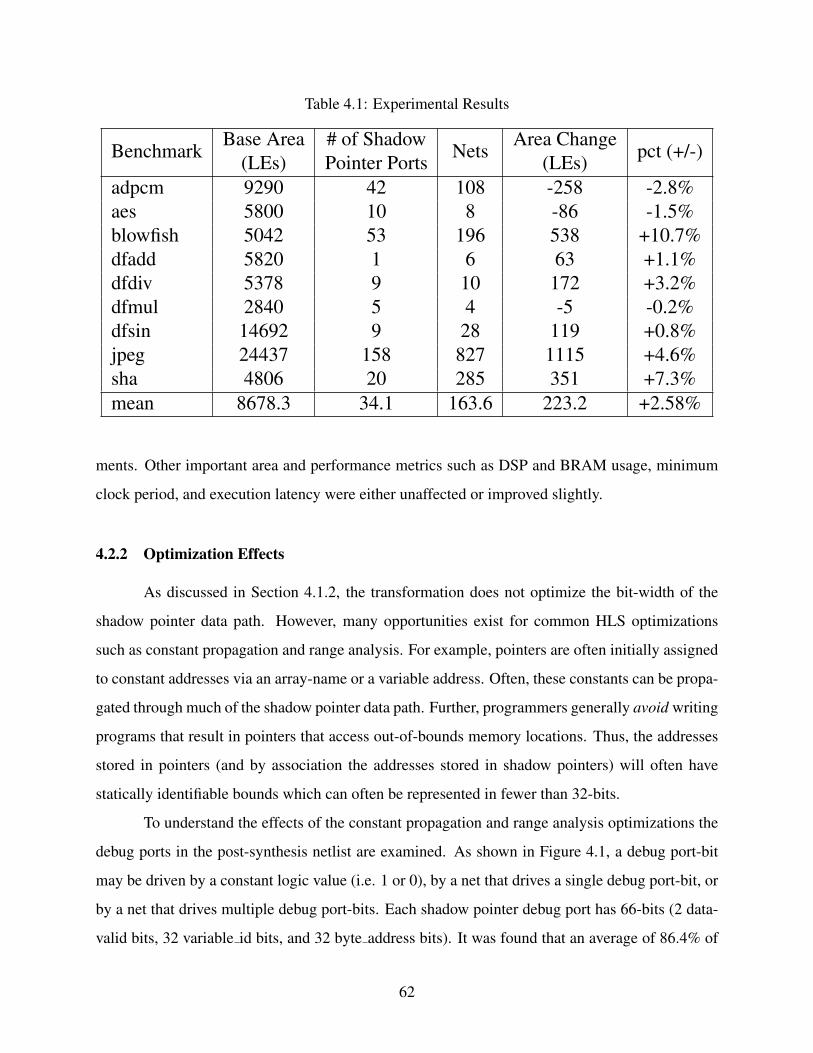
Table 4.1: Experimental Results
BenchmarkBase Area
(LEs)# of ShadowPointer Ports Nets
Area Change(LEs) pct (+/-)
adpcm 9290 42 108 -258 -2.8%aes 5800 10 8 -86 -1.5%blowfish 5042 53 196 538 +10.7%dfadd 5820 1 6 63 +1.1%dfdiv 5378 9 10 172 +3.2%dfmul 2840 5 4 -5 -0.2%dfsin 14692 9 28 119 +0.8%jpeg 24437 158 827 1115 +4.6%sha 4806 20 285 351 +7.3%mean 8678.3 34.1 163.6 223.2 +2.58%
ments. Other important area and performance metrics such as DSP and BRAM usage, minimum
clock period, and execution latency were either unaffected or improved slightly.
4.2.2 Optimization Effects
As discussed in Section 4.1.2, the transformation does not optimize the bit-width of the
shadow pointer data path. However, many opportunities exist for common HLS optimizations
such as constant propagation and range analysis. For example, pointers are often initially assigned
to constant addresses via an array-name or a variable address. Often, these constants can be propa-
gated through much of the shadow pointer data path. Further, programmers generally avoid writing
programs that result in pointers that access out-of-bounds memory locations. Thus, the addresses
stored in pointers (and by association the addresses stored in shadow pointers) will often have
statically identifiable bounds which can often be represented in fewer than 32-bits.
To understand the effects of the constant propagation and range analysis optimizations the
debug ports in the post-synthesis netlist are examined. As shown in Figure 4.1, a debug port-bit
may be driven by a constant logic value (i.e. 1 or 0), by a net that drives a single debug port-bit, or
by a net that drives multiple debug port-bits. Each shadow pointer debug port has 66-bits (2 data-
valid bits, 32 variable id bits, and 32 byte address bits). It was found that an average of 86.4% of
62

Shadow Pointer Data Path Registers
0
1
2
3
4
5
6
7
Debug Port
0
1
Net Driving Multiple Port-Bits
Portion of HLS-Generated Module
ELA
Nets Driving 1 Port-Bits
Constants Driving Port Bits
With Appropriate Book-Keeping There is no Need to Connect an ELA to These
Debug Port
Figure 4.1: Example of Connecting the Shadow Pointer Data Path to an ELA.
the shadow pointer debug port bits were driven by constant values. After accounting for nets that
drive multiple port bits, it was found that an average of 92.8% of the bit-width of the data path had
been optimized away. This means that, on average, 4 or 5 nets drive the non-constant bits of each
shadow pointer debug port.
As shown in Table 4.1, the designs with the highest area overhead (blowfish, jpeg, sha), also
had the highest numbers of nets driving the corresponding debug ports. However, in adpcm, which
had the fourth highest number of nets, a 2% improvement in circuit area was observed. It may seem
strange that adding logic for shadow pointers could result in an improvement in area. This can
occur because the HLS tool may choose to optimize the transformed source differently (for better
or for worse) than the non-transformed source. For example, in adpcm, Vivado HLS decided not
to inline a function from the transformed source that was inlined in the non-transformed source.
Since inlining a function results in an increase in area (it duplicates resources) a decrease in area
should be observed when a function call is not inlined (resources are no longer duplicated).
63

4.2.3 Any Room For Improvement?
While examining the three benchmarks with the highest area overhead (blowfish, jpeg, and
sha) it was found that each of the circuits had several shadow pointer byte-address ports with 32
unique, non-constant, port-bits. This was an indicator of potential shadow pointers that could not
be optimized by the range analysis or constant propagation. Upon close examination, however, it
was found that in each case the range of values the shadow pointer byte address could take was
statically determinable. However, the constant values that allowed the range to be determined
statically were outside of the given function. This indicates that the range analysis performed by
Vivado HLS was not context-sensitive (i.e. the analysis did not consider the calculated ranges of
function arguments). It was hypothesized that a context-sensitive range analysis would provide
additional area savings.
To test the hypothesis, the potential ranges of the five unoptimized byte-address ports in the
blowfish benchmark were calculated. Next, the design was modified to ensure that these shadow
pointers were only represented by the number of bits that had been determined. Once the mod-
ifications were complete the design was re-implemented. The modifications caused the design
overhead to drop by about 2.8%. Closer examination revealed that much of the remaining area
overhead was not part of the shadow pointer data path. A comparison of the IR of the transformed
and un-transformed benchmarks found that the insertion of debug ports was interfering with the
optimization of an if-statement (i.e. if-conversion). The source-code was manually modified to
insert the if-conversion (using a conditional expression, the ?: operator) and re-implemented in
Vivado HLS. The overhead of the resulting circuit dropped by another 6.1% (from 9.1% to 3.0%).
Based upon these manually-produced results, future work could investigate the modification of the
source-to-source compiler to automatically apply these transformations.
4.3 Conclusion
The shadow pointer transformation presented in this chapter filled in an important observ-
ability gap in the debug port transformation. In particular, it allows changes in source-level variable
values to be tracked even when that variable is modified indirectly (through a pointer). Prior to this
transformation there was no means of identifying which variables were modified indirectly through
64

pointers. This chapter also demonstrated that very often much of the additional logic added by the
debug port transformation was optimized to constant values. This occurred because many of the
pointers in the source only pointed to limited numbers of source-level variables. The HLS and logic
synthesis tools were able to take advantage of these facts and optimize the circuits to constants.
65

CHAPTER 5. MIGRATING TRANSFORMATIONS TO LEGUP
The transformations presented thus far in this dissertation have all been implemented and
tested on a single HLS tool, Vivado HLS. In this chapter the source-to-source compiler is updated
to support both Vivado HLS and another HLS tool – LegUp [13]. This requires making any nec-
essary modifications to ensure that both the compiler and transformations (debug port and shadow
pointer) are compatible with both tools. From a research perspective, migrating the transformations
to LegUp provides the opportunity to examine the portability of the transformations and catalog
any modifications that need to be made when porting transformations between HLS tools. As far
as the author of this dissertation is aware, no other works have reported on the results of migrating
a source-to-source transformation from one HLS tool to another. This is considered one of the
contributions of this dissertation. As will be shown, very few changes were required to achieve a
working version of the debug port transformation in LegUp. However, in the current version of
LegUp each write to a debug port comes at a cost of two additional cycles. When a large number
of expressions are instrumented the execution time of the instrumented circuit is significantly ex-
tended. To mitigate the additional latency a new approach for binding expressions to debug ports
is presented and shown to significantly reduce the excessive latency.
5.1 Primary Differences between Vivado HLS and LegUp
To motivate the discussion on porting transformations between Vivado HLS and LegUp
this section examines the primary differences between these tools. The following discussion will
describe both HLS tools and contrast their relevant differences.
5.1.1 LegUp
LegUp is an academic research tool out of the University of Toronto with the stated goal
to “broaden the FPGA user base to include software engineers” [13]. As such, LegUp generates
66

complete hardware systems from ANSI C programs. This allows software engineers to use LegUp
without any hardware design knowledge. LegUp supports two primary flows: pure hardware and
hybrid. The pure hardware flow compiles the entire C program (including main) to a hardware
accelerator. Test vectors are hard-coded into the program as global variables; these are synthe-
sized in block rams contained in a centralized memory controller at the top level of the design.
Descendant functions that access the global variables must send requests up the function hierarchy
to the memory controller. In the hybrid flow the user specifies functions for LegUp to implement
as hardware accelerators. The remaining functions are executed on a MIPS or ARM processor.
Communication between the processor and accelerator occurs primarily through either the proces-
sor’s local cache or main memory (when a cache miss is encountered). In both flows the only I/O
in LegUp accelerators is through a centralized memory controller.
The latest version of LegUp, version 4.0, was released recently [22]. LegUp 4.0 contains
the source-level debugging frame-works of both Goeders and Wilton [26] [27] [8] and Calagar et.
al [9]. To be clear, the goal of this chapter is not to propose a replacement for the source-level
debugging framework already provided with LegUp; rather it merely demonstrates that the source-
to-source debugging transformations proposed in this dissertation can be used in multiple HLS
tools. With the release of LegUp 4.0, the LegUp team has added several features that relax the
constraints on the system environment. First, LegUp now allows the user to specify a custom top-
level module. This allows users to include hardware components other than the processor, bus, and
LegUp-generated accelerators. Second, LegUp now supports user-defined I/O through the use of
custom Verilog module function implementations. These custom Verilog implementations allow a
user to replace a LegUp-generated function with a user-supplied Verilog module. Further, LegUp
will propagate any I/O ports from the custom Verilog module to the top level of the hardware
accelerator. With these two additional features a LegUp design could receive (send) data from (to)
other hardware components or even receive data from off-chip sources without having to request it
through the memory controller. In particular, these two new LegUp features provided a mechanism
through which the debug port transformation could be supported in LegUp.
67

5.1.2 Xilinx Vivado HLS
In contrast, Vivado HLS has always been focused on generating high-performance IP cores
for arbitrary system environments. As such, it does not assume a system model and does not
generate a complete system. This provides a lot of flexibility for hardware engineers but makes
it a difficult tool for software engineers to use without the support of a constrained environment
or an experienced hardware engineer. Thus the tool has historically been used to increase the
productivity of hardware engineers. Much of the flexibility comes from the wide variety of I/O
standards supported by Vivado HLS that allow the generated module to be easily integrated into any
arbitrary hardware system. However, in an effort to expand its user-base, Xilinx has been working
on higher-level tools that use Vivado HLS as a back-end to compile C programs to specific board
environments [?] [17]. The recent transitions made by both LegUp and Vivado HLS demonstrate
the importance of HLS tools supporting both arbitrary and constrained system environments.
5.2 Source-to-Source Compiler Architecture
The source-to-source compiler is designed in modular fashion that facilitates the testing
and evaluation of different strategies of implementing the primary components of the compiler. As
shown in Figure 5.1, the compiler consists of three swappable components. The functionality of
these components is described as follows:
1. Expression Selector: Analyzes the AST and creates a list of expressions that will be instru-
mented with debug ports.
2. Debug Port Binder: Analyzes the list of expressions chosen by the selector, allocates debug
ports, and assigns each expression to a debug port. Assigning an expression to a debug port
communicates to the instrumentor that it should instrument the code so that the result of the
expression is written to the assigned debug port.
3. Instrumentor: Modifies the AST of the program to insert debug ports and instrument
expressions according to the debug port-expression bindings generated by the debug port
binder.
68

TransformedSource Code
Input Source Code
Parser UnparserSelector Binder Instrumentor
Swappable Components
Source-To-Source Compiler
Figure 5.1: Architecture of the source-to-source compiler.
The modular structure of the source code of the source-to-source compiler allows users to
develop new strategies by creating a new C++ class that implements that strategy. The strategy can
then be loaded (in place of the default strategy) using command line arguments. For example, to
support the debug port transformation in LegUp a new Instrumentor class was created that used
LegUp specific syntax to insert debug ports and instrument expressions. This new functionality
was added without modifying the debug port binder or expression selection components.
5.3 Migrating Transformations to LegUp
Several changes were required to migrate the debug port transformations to LegUp (no
changes were required for the shadow pointer transformation). The primary reason for these
changes is that top-level I/O ports are defined and used very differently in LegUp than they are
in Vivado HLS. To illustrate the syntactical differences of creating a debug port, Listing 5.1 pro-
vides a juxtaposition of how a debug port is created in Vivado HLS versus how the same debug
port is created in LegUp. Lines 1 - 4 in Listing 5.1 show the uninstrumented function. Lines 6
- 11 show how this function is instrumented in Vivado HLS and lines 13 - 21 show the how the
same function is instrumented in LegUp. In terms of inserting a debug port, the primary differ-
ence between LegUp and Vivado HLS is the syntax used to declare a debug port and connect it
to an expression. As discussed in Section 3.1.1, the syntax used to insert a debug port in Vivado
HLS was to declare a global variable and add a pragma that instructs Vivado HLS to interpret the
declared global as a top-level port (as shown in lines 7, 10). The instrumented expression is then
69

“connected” to the debug port by inserting an assignment from the instrumented expression to the
global variable (representing the debug port).
LISTINGS 5.1: Examples of Vivado HLS and LegUp Transformations
1 / / o r i g i n a l code
2 i n t mul t ( i n t a , i n t b ){
3 re turn ( a * b ) ;
4 }
5
6 / / V ivado HLS Approach
7 i n t d b g p o r t 0 ;
8 i n t mul t ( i n t a , i n t b ){
9 #pragma HLS i n t e r f a c e p o r t = d b g p o r t 0
10 re turn ( d b g p o r t 0 = ( a * b ) ) ;
11 }
12
13 / / LegUp Approach
14 void a t t r i b u t e ( ( n o i n l i n e ) )
15 d b g p o r t 0 ( i n t a rg0 ){
16 p r i n t f ( ” DebugPor t0 :%d ” , a rg0 ) ;
17 }
18 i n t mul t ( i n t a , i n t b ){
19 i n t tmp0 ; / / , tmp1 ;
20 re turn ( tmp0 =( a *b ) , d b g p o r t 0 ( tmp0 ) , tmp0 ) ;
21 / / r e t u r n ( tmp0 =(a* tmp1=b ) , d b g p or t 0 ( tmp1 ) , tmp0 ) ;
22 }
In LegUp top-level ports are represented as functions as opposed to global variables (see
Listing 5.1 lines 14 - 17, 20). A debug port itself is specified by defining a new function in the
source code (lines 14-17) and adding a command in the configuration file associated with the
LegUp project. As shown on line 20, the connection between an expression and a debug port is
70

created by passing the result of the expression as an argument to the function. Special care must
be taken to ensure that LegUp properly instances the custom Verilog module within its generated
RTL. First, as shown on line 14, the noinline attribute must be added to the function definition
to ensure that calls to the function are not inlined (i.e. optimized away). Second, each function
parameter must be used as an argument to a print statement to ensure that the parameter is not
optimized away (see line 16).
The shift in the representation of a debug port from a global variable to a function required
that expressions no longer be implemented in place (i.e. within the original expression). Instead,
as shown on line 20 (Listing 5.1), the target expression (a * b), is instrumented by storing the result
of the expression into a temporary variable (tmp0, declared on line 19). The temporary variable is
then passed to the debug port function (dbgport0) which is appended to the statement using the
comma operator. Finally, the temporary variable is appended to the statement to ensure that the
return statement returns its intended value. In this case, the target expression (a * b) and the return
value of the statement were the same. The commented code on lines 19 and 21 shows how the
same statement would need to be instrumented if the target expression were b instead of (a * b).
As shown in the commented code on line 19, a second temporary variable (tmp1) would need to be
created. In this case, as shown in the commented code on line 21, tmp0 is used to store the value
passed to the return statement while tmp1 is used to store the result of the target expression. tmp1
is then passed to the debug port function while tmp0 is appended to the end of the statement to be
used as the operand for the return statement. The same approaches for ensuring the correctness of
the debug port transformation in LegUp are applied in other similar situations (e.g. conditionals of
if-statements and loops).
5.3.1 Using Custom Verilog Modules to Implement Debug Ports in LegUp
This subsection describes how LegUp’s “Custom Verilog Module” functionality is used to
implement debug ports in LegUp. As shown in Figure 5.2, data is generally moved into and out
of an accelerator through the memory controller at the top-level of a LegUp accelerator. However,
as shown, other top-level ports can be added as long as those ports are propagated from so-called
“custom Verilog modules”. This subsection will first discuss the architecture of a LegUp accel-
71

User-defined I/O
Ports
Insert CustomRTL Here
External Data Sources
LEGUP ACCELERATORTOP LEVEL RTL
main() RTL Module
foo() RTLModule Instance
Memory Controller
State Machine
andData Path
goo() Custom Verilog
Module Instance
bar() RTLModule Instance
Figure 5.2: Structure of Legup Accelerator RTL.
erator and then describe how “custom Verilog modules” fit into that architecture. Finally, this
subsection provides an example of a custom Verilog module that implements a debug port.
In LegUp (and most other HLS tools), an RTL module is generated for each function not
inlined during high-level synthesis. As shown in Figure 5.2, the top-level module of a LegUp ac-
celerator contains the RTL implementation of the main() function and the the memory controller.
As shown in the figure, the RTL module implementing main() includes a data path and state
machine (described using Verilog statements) and instances of the RTL modules that implement
functions called by main() (i.e. foo(), bar(), and goo()). With the possible exception of the
custom Verilog module (i.e. goo()), each of the RTL modules instanced in main() has the same
structure as main(), that is, a data path, state machine, and a set of RTL module instances. As
might be expected, this causes the RTL module instance hierarchy to closely resemble the function
call hierarchy of the source code.
72

LegUp does not generate RTL modules for functions specified as custom Verilog modules
(in the LegUp project configuration file); rather, it simply generates a module instance within the
RTL implementation of the calling function and relies on the user to supply the RTL implemen-
tation of the custom Verilog module. LegUp also provides a mechanism that allows the user to
add user-defined ports (i.e. those not automatically generated by LegUp) to the module instance of
a custom Verilog module. LegUp will then connect the user-defined ports on the custom Verilog
module instance to top-level ports of the LegUp accelerator. For example, in Figure 5.2, function
goo() is specified as a custom Verilog module. As shown in the figure, apart from its connection
to the memory controller through main()’s data path, goo() is also directly connected to I/O ports
at the top level of the LegUp accelerator. Note that even though only one level of module hierarchy
is shown in Figure 5.2, LegUp will propagate user-defined I/O ports through as many levels of
hierarchy as necessary.
LISTINGS 5.2: Custom Verilog Module for Debug Port Function in Listing 5.1
1 / / Legup C o n f i g u r a t i o n F i l e E n t r y
2 s e t c u s t o m v e r i l o g f u n c t i o n ” d b g p o r t 0 ” noMemory \
3 output 0 : 0 a r g 0 v a l i d o u t \
4 output 31 :0 a r g 0 o u t \
5
6 / / Custom V e r i l o g Module RTL f o r Debug Por t
7 module d b g p o r t 0 (
8 / * R e q u i r e d S i g n a l s * /
9 s t a r t , f i n i s h ,
10 c lk , c lk2x , c l k 1 x f o l l o w e r , r e s e t ,
11 / * F u n c t i o n Parameter * /
12 a r g 0 a r g ,
13 / * Propagated t o Top−L e v e l P o r t s * /
14 a r g 0 v a l i d o u t ,
15 a r g 0 o u t
16 ) ;
73

17
18 input s t a r t , c lk , c lk2x , c l k 1 x f o l l o w e r , r e s e t ;
19 output f i n i s h ;
20 input [ 3 1 : 0 ] a r g 0 a r g ;
21 output [ 3 1 : 0 ] a r g 0 o u t ;
22 output a r g 0 v a l i d o u t ;
23
24 a s s i g n a r g 0 o u t = a r g 0 a r g ;
25 a s s i g n a r g 0 v a l i d o u t = s t a r t ;
26 a s s i g n f i n i s h = 1 ’ b1 ;
27
28 endmodule
As an example, Listing 5.2 shows the required configuration file command (lines 1 - 4)
and the RTL (lines 6 - 28) for a custom Verilog module that implements the debug port func-
tion (dbgport0()) from Listing 5.1. As shown, the set custom verilog function command (on
line 2) instructs LegUp to use a user-supplied RTL module (custom Verilog module) for function
dbgport0() instead of generating an RTL module. Further, the command specifies that the custom
RTL does not need access to the memory controller (noMemory) and specifies that ports arg0 out
(line 3) and arg0 valid out (line 4) (the user-defined ports) on the custom Verilog module (lines 14,
15, 21, 22) be propagated through the Verilog module hierarchy and connected to similarly-named
ports at the top level of the accelerator. The start, reset, clk, clk1x follower, clk2x and finish (lines
9, 10, 18, 19) are signals required to properly integrate the custom Verilog module with the LegUp
accelerator. As one might expect, the clock and reset ports expose the accelerator’s clock and reset
signals to the custom Verilog module. The start and finish signals provide a means for the LegUp
accelerator to pass execution control to the custom RTL (start) and for the custom RTL to return
execution control to the accelerator (finish). The start signal also serves to validate the data input
(function parameter) of the custom Verilog module. LegUp requires that signals corresponding to
function parameters have the same name as the function parameter with the post-fix arg. For ex-
ample, arg0 arg (Listing 5.2, lines 12, 20) corresponds to arg0, the only parameter of dbgport0()
(Listing 5.1, line 15).
74
The primary functionality of the RTL implementation of dbgport0() is to connect the
input signal corresponding to the function parameter (ultimately the target expression) to the user-
defined port that is routed to the top-level of the design (arg0 out). This occurs on line 24 of List-
ing 5.2 where arg0 arg the function parameter (target expression) is assigned to arg0 out (which
LegUp routes to the top-level of the accelerator). A valid signal for the target expression is pro-
vided by connecting the start signal to arg valid out which is also routed to the top-level. Finally,
the finish signal is set to a logical ’1’ to ensure that the modules passes execution control back to
the accelerator as quickly as possible (two clock cycles) [22].
5.3.2 Compiler Modifications to Support LegUp
To provide LegUp support for the debug port transformation a new instrumentor component
(see Section 5.2) was created for the source-to-source compiler. The new component applies the
necessary transformations to define debug port functions and call them in the data paths of the
source code. It also generates the required configuration file and a Verilog file that contains the
RTL implementations of all debug port functions. The Verilog file is then automatically included
into the LegUp accelerator via an ‘include statement inserted by LegUp.
5.4 Improvements to Port-Binding Strategy
The primary challenge of supporting the debug port transformation for LegUp is the two
clock cycles of latency overhead incurred each time the result of an expression is written to a debug
port (i.e. the debug port function is called). In some cases, this latency overhead can significantly
affect the performance of an accelerator. This is especially true when large numbers of expressions
are instrumented or when expressions are instrumented within loop bodies. In some debugging
scenarios, large amounts of latency overhead may be tolerable; however, in others the accelerator
may not be able to operate fast enough to keep up with incoming data. While this latency overhead
cannot be eliminated, it can be reduced by lowering the number of expressions instrumented or only
instrumenting expressions outside of loops. Unfortunately, these approaches also tend to reduce
the number of expressions that can be observed by a debugging instrument (e.g. an ELA). In this
section, a new approach for creating debug ports and assigning them to target expressions (i.e.
75

debug port binding, see Section 5.2) is presented. This approach attempts to reduce the number of
calls to debug ports without reducing the number of visible expressions.
5.4.1 Naive/Default Binding Approach
Up to this point, the debug port binding strategy employed by the source-to-source compiler
has been to assign each target expression to its own debug port. Listing 5.3 provides an example
of code from the adpcm benchmark that was instrumented for LegUp using the default binding
strategy. Note that the printf() statements in the debug port function definitions have been
omitted. In the listing, the original (uninstrumented) code is black, the code added by the source-
to-source compiler is blue, and comments are green. In this example, the target expressions are
the four (4) variable assignment operations found on lines 12 - 16. The default binder created
a debug port for each of the 4 target expressions. Then, the LegUp instrumentor appended the
debug port calls to the end of the statement enclosing the corresponding target expression. The
latency overhead resulting from the debug port function calls is 8 clock cycles. This latency occurs
regardless of where the debug port function calls are placed within the source code.
This strategy worked well for instrumenting circuits in Vivado HLS, because, unlike LegUp,
Vivado HLS has no automatic latency penalty associated with writing a value to a debug port (as
LegUp does). Further, in the vast majority of cases (above 90%), expressions in Vivado HLS
can be instrumented without increasing the latency of the schedule at all. Since latency is not in-
creased, the results of target expressions are often connected to a debug port without being stored
in a register thereby reducing the area requirements of the debugging solution. However, due to
the automatic two-cycle latency penalty, the default strategy did not work as well when the trans-
formations were ported to LegUp. For example, as will be shown, execution latency increased
an average of 3.70 times when the default binding strategy was applied. This occurs primarily
because the default binding strategy does not take the latency penalty into account.
5.4.2 Delayed Port-Binding Strategy
The delayed port-binding strategy was devised to reduce the latency overhead of the debug
port transformation in LegUp. This strategy assumes that all target expressions will first be stored
76

LISTINGS 5.3: Example of Code Instrumented Using Default Binding Strategy1 / * D e f a u l t B i n d i n g * /2 void a t t r i b u t e ( ( n o i n l i n e ) ) DbgPort0 ( i n t a rg0 ) { . . . }3 void a t t r i b u t e ( ( n o i n l i n e ) ) DbgPort1 ( i n t a rg0 ) { . . . }4 void a t t r i b u t e ( ( n o i n l i n e ) ) DbgPort2 ( i n t a rg0 ) { . . . }5 void a t t r i b u t e ( ( n o i n l i n e ) ) DbgPort3 ( i n t a rg0 ) { . . . }6 i n t f i l t e p ( i n t r l t 1 , i n t a l1 ,7 i n t r l t 2 , i n t a l 2 )8 {9 i n t t0 , t1 , t2 , t 3 ;
10 long p l ;11 long p l 2 ;12 ( t 0 = p l = 2* r l t 1 , DbgPort0 ( t 0 ) , t 0 ) ;13 ( t 1 = p l = ( ( long ) a l 1 ) * p l ,14 DbgPort1 ( t 1 ) , t 1 ) ;15 ( t 2 = p l 2 =2* r l t 2 , DbgPort2 ( t 2 ) , t 2 ) ;16 ( t 3 = p l +=( ( long ) a l 2 ) * p l 2 ,17 DbgPort3 ( t 3 ) , t 3 ) ;18 re turn ( i n t ) ( p l >> 15) ;19 }
into a unique temporary variable (i.e., one that won’t be assigned in any other statements). Making
this assumption allows the port-binder to delay writing the result of the target expression to a
debug port (i.e. passing it as an argument to a debug port function call). The ability to delay debug
port writes allows the debug port binder to assign multiple target expressions to each debug port.
Multiple target expressions can be simultaneously written to a debug port by adding arguments to
the function definition. To support the parallel writing of debug port arguments to top-level ports
the bit width of the debug port is increased. Thus the debug port itself can support an arbitrary
number of expressions without increasing the latency penalty. Sharing debug ports in this way has
the effect of reducing the number of debug port function calls while allowing the user to observe
the same number of target expressions. For example, if five (5) target expressions are each bound
to their own port, 10 cycles of latency will be added to the circuit. However, if these five target
expressions are bound to one debug port, only 2 cycles of latency will be added to the circuit.
There are limits on the debug ports to which a target expression can be assigned. This
limitation is based on the assumption that the result of an expression needs to be written to a debug
77

port each time it is executed. Two conditions must be met to guarantee that this is true. First, a
target expression must be assigned to a debug port that is called after the result of the expression
has been computed. Second, a target expression must be assigned to a debug port that is called
within the same code block as the target expression (i.e. within the same set of curly braces). For
example, if an expressions exists within the body of a loop it must be assigned to a debug port
that is called after the expression is executed but before the end of the loop body. If, the same
target expression was followed by a conditional break statement (i.e. a break statement within
an if-statement) the expression should be assigned to a debug port called prior to the conditional
break statement. However, with special handling, an expression within an if-statement block can
be assigned to a debug port that is called after the if-statement block. The only requirement is
that along with the result of the if-enclosed target expression the debug port also presents enough
information to determine whether the if-enclosed target expression was executed. This is done by
storing the results of any if-statement conditionals related to the execution of the target expression
and writing them to the debug port as well. This is important because a value will be written to the
debug port whether or not the if-enclosed target expression was executed. Together, the results of
related if-statement conditionals create a de facto valid signal for the if-enclosed target expression
at the debug port.
5.4.3 Delayed Binding Algorithm
As previously discussed the goal of the delayed binding approach is to reduce latency over-
head as much as possible. This can be accomplished by maximizing debug port sharing while
still obeying the two binding constraints discussed in the previous section. The delayed binding
strategy accomplishes these goals using the following process. The binder searches for the latest
point in the program where the result of each target expression can be written. This search begins
with the statement that encloses the target expression and continues through each subsequent state-
ment until a (closing) curly brace, loop statement, terminating statement (i.e. return, break,
continue, or exit()), or if-statement containing a terminating statement is encountered. If the
end of an if-statement body is encountered, the if-statement conditional is added to the list of target
expressions and eventually bound to the same debug port as the original target expression. Once
the latest point has been found, the binder checks whether it has already created a debug port that is
78

LISTINGS 5.4: Simple Example of Delayed Binding Approach1 / * S i mp le Delayed B i n d i n g Example * /2 void a t t r i b u t e ( ( n o i n l i n e ) ) DbgPort0 ( long , long ,3 long , long ) { . . . }4 i n t f i l t e p ( i n t r l t 1 , i n t a l1 ,5 i n t r l t 2 , i n t a l 2 )6 {7 long t0 , t1 , t2 , t 3 ;8 long p l ;9 long p l 2 ;
10 t 0 = p l = 2 * r l t 1 ;11 t 1 = p l = ( ( long ) a l 1 ) * p l ;12 t 2 = p l 2 = 2 * r l t 2 ;13 t 3 = p l += ( ( long ) a l 2 ) * p l 2 ;14 DbgPort0 ( t0 , t1 , t2 , t 3 ) ;15 re turn ( i n t ) ( p l >> 15) ;16 }
called at this point in the program. If a debug port has been created, the target expression is bound
to that debug port. Otherwise, the binder creates a new debug port and binds the target expression
to it. The result of this process is that most target expressions are collected into a single debug port
at the end of the enclosing loop or function body.
Listing 5.4 shows a simple example of the delayed binding approach. This listing follows
the same text-color scheme found in Listing 5.3, that is, the original uninstrumented code is black,
code added by the source-to-source compiler is blue, and comments are high-lighted in green. In
order to contrast the default and delayed binding approaches, both Listing 5.3 and the example in
Listing 5.4 show instrumented versions of the same function (filtep()) from the adpcm bench-
mark. However, the example in Listing 5.3 used the default binding approach to instrument the
code while the example in Listing 5.4 used the delayed binding approach.
The primary difference between the two examples is the number of debug ports that were
created and the amount of latency overhead that was incurred. In Listing 5.3, 4 target expressions
were instrumented and 4 debug ports were created resulting in 8 cycles of latency overhead. On the
other hand, as shown in Listing 5.4, the delayed binding approach bound the 4 target expressions
to a single debug port called just prior to the return statement (line 14). By calling only 1 debug
79

LISTINGS 5.5: Complex Example of Delayed Binding Approach1 / * Complex Delayed B i n d i n g Example * /2 void a t t r i b u t e ( ( n o i n l i n e ) ) DbgPort0 ( long ) { . . . }3 void a t t r i b u t e ( ( n o i n l i n e ) ) DbgPort1 ( i n t , long ) { . . . }4 void a t t r i b u t e ( ( n o i n l i n e ) ) DbgPort2 ( i n t , i n t , i n t ) { . . . }5 i n t q u a n t l ( i n t e l , i n t d e t l )6 {7 long wd , d e c i s , t0 , t 2 ;8 i n t r i l , mi l , t1 , t3 , t4 , t 5 ;9
10 t 0 = wd = ( abs ( e l ) ) ;11 DbgPort0 ( t 0 ) ;12 f o r ( mi l = 0 ; mi l < 3 0 ; mi l ++) {13 t 1 = mi l ;14 t 2 = d e c i s = ( ( d e c i s l e v l [ mi l ] * ( ( long ) d e t l ) ) >> 15L ) ;15 DbgPort1 ( t1 , t 2 ) ;16 i f ( wd <= d e c i s ) {17 break ;18 }19 / * DbgPort1 ( t1 , t 2 ) ; * /20 }21 i f ( t 3 = e l >= 0) {22 t 4 = r i l = q u a n t 2 6 b t p o s [ mi l ] ;23 / * DbgPort3 ( t 4 ) ; * /24 } e l s e {25 t 5 = r i l = q u a n t 2 6 b t n e g [ mi l ] ;26 / * DbgPort4 ( t 5 ) ; * /27 }28 DbgPort2 ( t3 , t4 , t 5 ) ;29 re turn r i l ;30 }
port, the latency overhead was only 2 clock cycles. This is a significant improvement over the
8 cycles that resulted from the default binding approach. Further, the delayed binding approach
accomplished this while instrumenting the same target expressions as the default binding approach.
However, the 1 debug port added by the delayed binding approach is roughly 4 times wider (in
terms of bit width) than any single port created by the default binding approach. This being said, in
total, the delayed binding approach actually creates 3 less debug port bits than the default approach
because it only requires a valid signal for 1 debug port instead of 4.
80

To illustrate some of the more complex details of the delayed binding approach another
example has been included as Listing 5.5. Recall that part of the delayed binding approach is to
search for the latest point in the source code that a call to a debug port function can be inserted
while still ensuring that all instances of a target expression are written to the debug port. This
principal is illustrated by DbgPort0 and DbgPort1 which are debug port functions called on lines
11 and 15 respectively. DbgPort0 was called on line 11 because of the for loop statement on line
12. Technically, the call to DbgPort0 could have been delayed and merged with DbgPort2 while
still ensuring that the value was written. However, this may not be good practice as delaying the
call to DbgPort0 would cause the expressions in the body of the loop (DbgPort1) to be written
before the expressions in DbgPort0. Further, deadlock is a common problem with HLS designs
and delaying the write of the expressions associated with DbgPort0 until after a loop (especially
a long loop) increases the probability of encountering a deadlock condition before the expression
can be written to the debug port. This is a challenge because the result of the expression may
contain critical information for debugging the deadlock. The challenges and possible solutions to
the deadlock problem for the delayed binding approach will be discussed in more detail in Section
5.4.4.
The insertion point of the call to DbgPort1 (line 15) illustrates why the debug port write
must be inserted prior to conditional break statements (i.e. a break statement inside of an if state-
ment, see lines 16 - 18). First, consider the situation if DbgPort1 had been placed after the con-
ditional break statement (as illustrated by the commented code on line 19) and not before. Using
this insertion point the expressions captured by temporary variables t1 and t2 (assigned on lines
13 and 14) would be written to the debug ports on all iterations except for iterations where the
conditional break point is taken. This situation is avoided by inserting the call to DbgPort1 prior
to the conditional break point.
Finally, DbgPort2 (called on line 28) illustrates the how target expressions enclosed by if-
statement bodies (e.g. lines 22 and 25) are instrumented outside of those same function bodies. As
previously discussed, this is accomplished by storing the result of the if-statement conditional into
a temporary variable (line 21) and writing it to the same debug port as the if-enclosed target ex-
pressions (i.e. DbgPort2, line 28). The alternative to writing the results of if-enclosed expressions
outside of if statements is to write them within the if-statements as shown by the commented code
81

on lines 23 and 26. In many cases, (but not this one), this alternative leads to more latency over-
head than is necessary. In this case, using the alternative instrumentation approach would result in
only one debug port being called in this section of code each time the function is executed. This
is because the alternative removes the need for DbgPort2 and the if-statement ensures that only
DbgPort3 or DbgPort4 would be called. However, in the general case, other target expressions
either before or after the if-statement would require DbgPort2 to be inserted.
5.4.4 Debugging Deadlock using the Delayed Binding Approach
As previously discussed, deadlock is a common problem when debugging in HLS gener-
ated circuits. Deadlock errors can often be difficult to debug since the only symptom is that the
circuit stops working. Deadlock generally occurs within an HLS design when the HLS-generated
circuit attempts a read from an external circuit and that read is not or cannot be fulfilled. For exam-
ple, poorly-sized streaming FIFOs are a common source of deadlock within Vivado HLS generated
circuit. Another example occurs when the HLS-generated circuit makes an erroneous read-request
that cannot be fulfilled by the surrounding system (e.g. attempting to read a non-existent memory
address). Deadlock errors are often encountered while integrating an HLS circuit into an existing
system.
The deadlock issue poses a particular problem for the delayed binding approach. This is
because the delayed binding approach may separate the execution of a target expression from the
operation that writes its result to the debug port. If they are separated by one or more clock cycles,
it is possible that an intervening operation may deadlock; thus, preventing the result of the target
expression from ever being written to the debug port. This complicates the debugging process
especially if the target expression would have provided useful debugging information.
In general, the programming constructs that can cause deadlock are usually easily identifi-
able. For example, reads from streaming FIFOs, external memory accesses, and synchronization
commands can be easily identified in the source code. If deadlock is a concern, the delayed binding
strategy could be updated to treat these constructs in the same way it treats curly braces, that is,
program points at which writes to debug ports can no longer be delayed and must be written. Such
an approach would likely ensure that all debug port values computed prior to the dead lock would
be available for inspection by the developer should a deadlock occur.
82

Src.-to-Src.Compiler
Initial C Code
Transformed C-Code
VivadoHLS
2014.1
Vivado2014.1
Legup 4.0 Quartus13.0
Vivado HLS Simulation
ModelSim
Configuration
Figure 5.3: Experimental Flow for Legup and Vivado HLS designs.
5.5 Experiments and Results
5.5.1 Experiments
Several experiments were performed to evaluate the effectiveness of the debug port and
shadow pointer transformations in LegUp. To facilitate comparisons with Vivado HLS the 9 CH-
Stone benchmarks [60] that are synthesizable by Vivado HLS [1] [2] were used. In general, the
experiments were carried out using the experimental flow detailed in Figure 5.3. First, the initial
source-code for each benchmark was passed to the source-to-source compiler along with a con-
figuration. The configuration specified which internal components the source-to-source compiler
should use (i.e. selector, binder, instrumentor). After the source-to-source compilation process was
complete, the transformed source code was passed to Vivado HLS or LegUp. The resulting RTL
was then passed to the FPGA vendor tool flow corresponding to the HLS tool. For LegUp the RTL
was passed to Quartus 13.0 and mapped to the Cyclone II. Vivado HLS designs were compiled for
a Zynq 7000 and built in Vivado 2014.1 using Vivado HLS’s built in export functionality.
By default, the Quartus projects generated by LegUp use extremely tight clock constraints
(e.g. 2 ns clock period). It is assumed that this is done to direct Quartus to try to hit the highest
clock rate possible. For many of the benchmarks, this approach worked; while they did not meet
the specified clock rate (i.e. 500 MHz) they compiled with clock periods comparable to those of the
un-instrumented designs. However, for some of the benchmarks, (especially the larger benchmarks
dfsin and jpeg), this approach led to long compile times and eventual failure. This occurred even
83

though the benchmarks were small enough to fit on the device. When necessary, the problem was
mitigated by loosening the clock constraints to 20 or 40 ns. Even though the clock constraints
were loosened, the benchmarks still achieved maximum clock frequencies similar to or better than
those achieved by the uninstrumented baseline circuits. In one variant of the jpeg benchmark
(delayed binding with pointers) loosening the clock constraints was not enough. However, the
design compiled easily when the circuit was moved to a larger Cyclone III device.
5.5.2 Results
With the one noted exception, all source-level transformations were successfully compiled
by LegUp and implemented in Quartus. The implemented designs were simulated to double-check
that the transformations did not affect the functional correctness of the circuits. This section de-
scribes a variety of experimental results and details how the source-level transformations impacted
circuit latency and area. The LegUp and Vivado HLS results are presented relative to uninstru-
mented baseline circuits compiled using the default settings of the respective HLS tool.
5.5.3 Effect of Delayed-Binding Strategy
The delayed-binding strategy is a technique that bundles debug ports together in a way that
minimized their latency impacts (see Section 5.4). The first series of experiments measures the
worst-case impact of this optimization by instrumenting all assignment expressions and building
the benchmarks using two different binding schemes: (1) the default, unbundled approach, and
(2) the bundled, delayed-binding approach. The results of these experiments are found in Table
5.1. The measured average increase in latency for the default approach, shown in the first column
of Table 5.1, is 3.70X. In the three most extreme cases (adpcm, dfadd, dfmul) latency increases
between 6-8 times. The default binder also resulted in a 72% average increase in area (Table
5.2). As shown in the next column of Table 5.1, the delayed-binding strategy reduced the latency
overhead from 3.70X to 1.95X and decreased area overhead slightly, from 72% to 69%.
84

Table 5.1: Simulation Latency Overhead
Legup Vivado HLS
benchmarks Default Delayed BindingDelayed Binding
w/Pointers DefaultDefault
w/ Pointersadpcm 7.09 2.82 3.51 0.85 0.85aes 4.44 1.49 1.49 1.15 1.15blowfish 2.23 1.28 1.28 1.00 1.00dfadd 5.83 3.24 3.24 1.33 1.33dfdiv 2.46 1.54 1.54 1.00 1.00dfmul 7.09 3.66 3.66 0.94 0.94dfsin 3.00 1.76 1.76 1.01 1.01jpeg 1.87 1.54 1.61 1.00 1.00sha 3.25 1.55 1.55 1.00 1.00Average 3.70 1.95 2.01 1.02 1.02
Table 5.2: Area Overhead (LEs)
Legup Vivado HLS
benchmarks Default Delayed BindingDelayed Binding
w/ Pointers DefaultDefault w/Pointers
adpcm 1.10 1.35 1.12 1.25 1.24aes 1.61 1.45 1.45 1.19 1.19blowfish 1.52 1.51 1.60 1.53 1.62dfadd 2.01 2.09 2.08 1.14 1.14dfdiv 1.88 1.64 1.63 1.26 1.24dfmul 2.60 2.47 2.48 1.09 1.09dfsin 1.88 1.71 1.72 1.31 1.30jpeg 1.03 1.02 1.16 1.22 1.29sha 2.62 2.55 2.63 1.25 1.33average 1.72 1.69 1.78 1.24 1.26
5.5.4 Latency Overhead
The previous experiments measure the worst-case latency caused by inserting debug ports
on all possible expressions. However, in actual practice, engineers will often want to focus their
debugging activities on specific sections of the circuit and hence will only instrument smaller
subsections of a circuit at a time. In other cases, vendors of FPGA-based products may desire to
permanently install instrumentation in the final product so they can perform additional tuning and
debugging in the field.
85

In general, inserting debug ports using using the previously-discussed source transforma-
tions results in two types of latency overhead. The first type, debug-port latency, is the two-cycle
overhead that results from calling debug port functions in LegUp. The second type, scheduling
latency, arises when the insertion of a debug ports alters the optimization and scheduling of the de-
sign. By profiling the simulation results it was found that, on-average, 80% of the latency overhead
in the previous experiment was a result of debug-port latency while 20% resulted from scheduling
latency.
Figure 5.4 illustrates how total debug-port latency is likely to change as different numbers
of debug ports are inserted into a design. The figure was created by profiling the debug-port activity
during the simulation of each of the fully-instrumented benchmarks, based on the delayed-binding
strategy. Profiling kept track of the total number of times each debug port was activated. The total
debug-port latency (for each benchmark) was found by summing the port-latencies of all of the
debug ports in the benchmark and placed as the first data-point in the top-left corner of Figure 5.4.
Subsequent data points were created by iteratively removing the debug port with the highest port-
latency until all debug ports are removed at the far right of the graph (100% of ports removed).
The trendline is a best-fit polynomial interpolation of all of the data for all benchmarks. The data
in Figure 5.4 represent the latency costs for debug-port latency (80% of all latency, on average) but
do not include the latency that may be caused by scheduling latency (responsible for 20% of all
latency, on average).
Three additional experiments were run to verify the accuracy of the results shown in Figure
5.4. In these experiments, the transformed source-code was modified to remove calls to a per-
centage of the debug port functions for all of the benchmark circuits. As before, the most active
debug ports were removed first. Once the ports were removed, the source-code was synthesized
with LegUp and the resulting RTL was simulated. The left-most red dot in Figure 5.4 shows the
results of the first experiment which removed the top most-active 10% of the debug ports. As
shown by the data point, removing the top 10% of the debug ports reduced the latency overhead
from 100% to 60%. This number represents the average latency measured across all benchmarks.
The next two red dots show the additional impact of removing 20% and 50% of the debug ports.
As expected, the data represented by the red-dots indicate that latency costs are slightly higher than
that predicted by the trend-line because the completely-synthesized results include both debug-port
86

10% Ports Removed
20% Ports Removed
50% Ports Removed
0%
10%
20%
30%
40%
50%
60%
70%
80%
90%
100%
0% 10% 20% 30% 40% 50% 60% 70% 80% 90% 100%
Percen
tage of R
emaining
Port‐Latency
Percent of Ports Removed
ADPCM
AES
BLOWFISH
DFADD
DFDIV
DFMUL
DFSIN
JPEG
SHA
TrendLine
Figure 5.4: Distribution of Latency Overhead
and scheduling latency. These experiments validate the previous findings regarding debug-port and
scheduling latency and indicate that the experimental approach shown in the figure is sufficient for
estimating latency increases caused by the insertion of individual debug ports.
In summary, the results displayed in Figure 5.4 suggest that, on average, the majority of
the latency overhead is caused by a relatively small number of ports, i.e., those with the highest
activity rates. For example, it was found that the top 20% of debug ports were responsible for 60%
of the total latency overhead while 80% of the ports were responsible for the remaining 40% of
the overhead. The top 20% of debug ports are classified as high-latency ports since together they
account for a majority of the latency, and each individual port will likely contribute significant
latency. On the other hand, the lower 80% of debug ports are classified as low-latency ports
because each port from this classification will account for only a small amount of latency. In
general, high-activity ports are found in loop bodies.
87

5.5.5 Cost of Individual Debug Ports
To provide a better sense of the latency cost of inserting individual ports with differing
activity rates, an additional series of experiments was conducted to confirm the total latency costs
(scheduling latency + debug-port latency) caused by inserting a single port in each of the bench-
marks. Three ports were selected for each benchmark, based upon the results from earlier experi-
ments: (1) the highest-activity debug-port, (2) the least-active debug port, and (3) a debug port on
the boundary between the high-latency ports (top 20%) and the low-latency ports (bottom 80%) as
described previously. Each benchmark was synthesized/implemented three times; a single one of
the three debug ports was inserted into the benchmark each time. The resulting circuits were built,
simulated and the latency increases were measured.
Table 5.3 shows the results of each of these experiments. On average, latency overhead
drops from an average of 20% to an average of 4% between the highest latency and boundary
debug ports. This suggests that the other high-latency ports are likely to have a latency overhead
somewhere between 4% and 20%. As one might expect the lowest latency port does not contribute
much to the latency overhead. Therefore, on average, it is expected that the low-latency ports (80%
of all ports) have a latency overhead of less than 4%. However, due to unpredictable scheduling
latency some of the low latency debug ports may have latency overhead greater than 4%. For
example, since debug ports are classified as low-latency or high-latency based on their port latency,
it is possible that the instrumentation of a randomly-selected low-latency debug port may result in
scheduling latency overhead that is somewhat higher than that predicted by the boundary overhead.
This is because the scheduling latency of any given debug port is not predictable.
The area costs of the highest-latency, boundary-latency, and lowest-latency are shown in
Table 5.4. The area impacts of these ports range from a small improvement to a 9% overhead.
On average, the individual port impacts ranged from 1%-2%. These results are comparable to the
results for Vivado HLS found during the feasibility study in Chapter 3. Recall that the feasibility
study found that the area overhead of individual debug ports centered on a small means (.3%) with
std. deviations of 1-3%; which appears to be similar to the results from LegUp.
88

Table 5.3: Latency Impact of Single Ports
benchmarks Highest Lat. Boundary Lat. Lowest Lat.adpcm 1.65 1.07 1.00aes 1.15 1.01 1.00blowfish 1.06 1.01 1.00dfadd 1.24 1.07 1.00dfdiv 1.04 1.01 1.00dfmul 1.29 1.12 1.01dfsin 1.07 1.01 1.00jpeg 1.09 1.01 1.00sha 1.16 1.05 1.00Average 1.20 1.04 1.00
Table 5.4: Area Impact of Single Ports
benchmarks Highest Lat. Boundary Lat. Lowest Lat.adpcm 0.97 1.00 1.01aes 1.01 1.00 1.00blowfish 1.02 1.05 1.00dfadd 1.05 1.09 1.04dfdiv 1.00 1.00 1.00dfmul 1.01 1.00 .99dfsin 1.04 1.02 1.02jpeg 1.01 1.00 1.01sha 1.02 1.00 1.00average 1.01 1.02 1.01
5.5.6 Comparison of LegUp and Vivado Results
Now that the transformations have been applied in both Vivado HLS and LegUp this section
compares and contrasts the results from the transformations applied in each tool. For convenience,
area and latency results from Vivado HLS have been appended to Tables 5.1 and 5.2 adjacent to the
LegUp results. Before beginning the comparison, some differences between the circuits generated
by Vivado HLS and LegUp need to be pointed out. First, the experiments performed in Chapter
3 used a different version of the CHStone benchmarks (v1.9) than the one available in LegUp;
additionally the CHStone benchmarks were modified slightly (as discussed in Chapter 3) to ensure
that I/O ports were added correctly. A programmatic comparison (diff) of the LegUp-native
CHStone and CHStone v1.9 revealed the differences are small. The primary change between the
89

newer and older versions is the way the self-checking mechanism reports results. The older version
(LegUp-native) reports the number of correct results while the newer version reports the number
of incorrect results. The second difference in the circuits generated by LegUp and Vivado HLS is
that LegUp synthesizes entire programs, including main(). This means that more functionality is
included in the LegUp results than Vivado HLS which does not synthesize main(). Finally, the
results were synthesized by different (logic) synthesis tools onto very different FPGA architectures.
Generally speaking, an in depth, benchmark-by-benchmark comparison of these circuits requires
a degree of experimental control which is far beyond the scope of this dissertation.
Some conclusions, however, can be drawn about the percentage change in area and latency
caused by the transformations in each tool. As shown in Table 5.1, the latency overhead in Vivado
HLS is almost non-existent. This is likely due to the Vivado HLS’s ability to schedule writes
to ports during the same clock cycles as other operations. Even after implementing the delayed
sharing technique the disparity between the latency overhead of LegUp and the latency overhead
in Vivado is significant ( 1.95X vs. 2%). On average, the LegUp transformations caused almost
three times more area increases than those caused by Vivado HLS. Increases in Vivado HLS ranged
from 0-30%. On the other hand, increases in LegUp ranged from 2% to 2.55X.
5.5.7 Impact of Instrumenting Pointers
It is interesting to note that the pointer transformation was run in both Vivado HLS and
LegUp without any modifications to the transformation. The latency and area results of running
the shadow pointer transformation along with the debug port transformations is shown in Tables
5.1 and 5.2. With the exception of adpcm (in LegUp), the pointer transformation had very little
impact on area and latency in either Vivado HLS or LegUp. Vivado HLS saw no increase in latency
(on average) and a 2% increase in area. LegUp, on the other hand, saw an average 6% increase
in latency and 4% increase in area. If the impact of jpeg is removed, which was unable to route
on the Cyclone II (although it could fit), an average 2% decrease in area with the addition of the
pointer transformation was observed. The small size of the impacts are likely due to the fact that
the relative number of pointers compared to other instrumented expressions is small (especially in
the floating point benchmarks, i.e. dfadd, dfdiv, dfmul, and dfsin). In addition, using the delayed
binding approach allowed many pointer expressions to be bound to already existing debug ports.
90

This avoided much of the additional latency. The adpcm benchmarks was an outlier in the fact that,
with the addition of the pointer transformation, it saw a large increase in latency and a significant
decrease in area. While the exact cause of this irregularity is unknown, it is likely that pointer
transformation caused the HLS tool to make different decisions in how it optimized the adpcm
benchmark. Similar effects were seen in previous results.
5.5.8 Usability and Feasibility
This chapter successfully demonstrates that a single tool can apply source-to-source compiler-
based transformations across multiple HLS tools. As reported, a single tool was created and this
tool successfully instrumented source code for two different HLS tools: LegUp and Xilinx’s Vi-
vado HLS. However, the source-to-source compilation approach also demonstrates that signifi-
cantly different impacts may occur when using different HLS tools. In particular, synthesizing
instrumented code with LegUp results in far more latency than when similarly instrumented code
is synthesized by Vivado. In the case where all possible expressions are instrumented, the increase
in latency may result in circuits that are too slow for effective debug in some situations. As was
shown, latency was not a concern when using Vivado HLS and it is not clear at this point whether
similar increases in latency will be seen when the tool is applied with other synthesis tools or if
LegUp will prove to be the outlier in this regard.
Setting aside latency concerns, it is still not generally desirable to instrument all possible
expressions in source code because of potential area impacts and because it will be difficult to cap-
ture a sufficient swath of data of sufficient depth when so many signals are being captured (many
thousands of bits). Most debugging scenarios are better served by more targeted instrumentation
and the tool disclosed in this paper makes it relatively easy for the user to control which expres-
sions are to be instrumented. As mentioned, it is not at all uncommon for shipping products to
contain some amount of instrumentation for later test and performance tuning. For these and other
scenarios, the latency costs of instrumenting smaller numbers of ports as shown in Tables 5.3 and
5.4 are feasibly low enough to be used for effective debugging. In some cases designers may still
desire to instrument all expressions if for no other reason than to eliminate the need to recompile
every time the user decides to observe a different set of expressions. For many circuits, latency
costs were about 1.5X those of the original, un-instrumented circuit (only for LegUp) and this may
91

not impede effective debugging in many cases; note that the current ELA-based debugging tools in
use with Verilog/VHDL circuits often consume a significant amount of area and also increase the
clock period a significant amount. Also, at least for the LegUp case, avoiding expressions that are
in oft-executed loops can dramatically lower the latency increase. Unfortunately, adding observ-
ability to hardware still has real costs relative to general software. Much of this added cost is due
to the fundamental difference between the computing models used by FPGAs and general-purpose
processors.
5.6 Conclusion
The objective of this chapter was to show that source-to-source transformations could be
effectively applied in two very different HLS tools: Vivado HLS and LegUp. These transforma-
tions had previously been demonstrated in Vivado HLS [1,2] but they had never been successfully
demonstrated in any other HLS tools. Migrating these transformations to LegUp required the de-
velopment of new components for the source-to-source compiler. The modular structure of the
source-to-source compiler allowed support for LegUp to be added using only 1502 new lines of
C++ code. The additional code included the LegUp-specific instrumentor (301 lines), supporting
code (680 lines), and the delayed binding component (521 lines).
Even though higher latency overhead (1.95X) was observed when debug ports were added
to observe all assignment expressions in a design, source-to-source transformations are still a rea-
sonable approach for real-world debugging scenarios in which small, targeted subsets of signals
are instrumented. In general, it was found that 80% of all debug ports, when instrumented individ-
ually, were likely to result in latency overhead of less than 4%. On the other hand, the remaining
20% were likely to result in a latency overhead of 4%-20% on average.
92

CHAPTER 6. MIGRATING TRANSFORMATIONS TO OTHER HLS TOOLS
In Chapter 5, it was shown that the source-to-source transformations presented in this paper
could be used in LegUp as well as Vivado HLS. Although, the transformations worked success-
fully, the instrumented hardware generated by LegUp exhibited significantly larger increases in
area and decreases in performance than the instrumented circuits generated by Vivado HLS. For
example, the average relative growth of LegUp circuit area (as a percentage) was 3 times that
which resulted from instrumenting Vivado HLS circuits (See Table 5.2). Unfortunately, the degra-
dation in performance – especially latency – and area may be significant enough to dissuade people
from using the source-to-source transformations presented in this paper to instrument their LegUp-
generated circuits for debug. The fact that the transformations worked well for Vivado HLS and
not-so-well for LegUp broaches three important questions: 1) What are the primary causes of the
disparities between the Vivado HLS and LegUp results? 2) What qualities or features does an
HLS tool need to be amenable for debug instrumentation via source-to-source transformation as
presented in this dissertation? 3) Are there any HLS tools (other than Vivado HLS) that could be
amenable to the source-to-source transformations presented in this dissertation?
6.1 Disparities between Vivado HLS and LegUp Results
When comparing Vivado HLS and LegUp it is important to remember that LegUp is an
open-source academic research tool primary written by graduate students. Due to limited time and
resources, it is likely that the authors of LegUp made careful decisions that simplified its imple-
mentation. For example, LegUp does not schedule operations from different basic blocks during
the same clock cycles even when doing so may be advantageous [22]. On the other hand, Xilinx
is heavily invested in Vivado HLS and likely has a large team of experienced engineers improving
and maintaining the tool. Thus, it is expected that Vivado HLS would utilize a larger number of
advanced features – such as concurrent scheduling of basic blocks – and generate smaller, higher
93

performing designs than LegUp. That being said, it is still possible to identify specific features that
may be causing the disparities between circuits generated by Vivado HLS and LegUp.
As previously discussed, the primary cause of the performance disparity is the two clock
cycles of port latency incurred each time a debug port function is called. This latency is incurred
because LegUp schedules all function calls under the assumption that the latency of the function
is unknown (even when the latency of a function is deterministic). Thus, it must add two control
states – one to start the function and one to wait until it completes – for each function call. Further,
LegUp does not schedule function calls in parallel with other function calls or operations even
when it is possible to do so. This ensures that each function call requires at least two clock cycles
to execute.
LegUp’s handling of function calls also increases the area of the final circuit (when instru-
mented for debug) in ways that do not always occur in Vivado HLS. First, the two control states
added to implement the debug port function call result in a larger FSM (requiring more LUTs and
FFs to implement). Second, it requires the creation of additional control logic (i.e. the start and
finish signals). Finally, it forces each value written to a debug port (i.e. used as an argument to
a debug port function) to be registered prior to being written to the debug port. In many cases,
such values are registered anyway. However, in some cases, such as when operations have been
chained, instrumentation will cause additional registers to be created.
6.2 Required HLS tool Support for Source-to-Source Transformations
In general, an HLS tool must support two features in order to efficiently use the source-
to-source transformations presented in this dissertation. These features are listed in the following
requirements:
• Requirement #1: The HLS tool must provide a mechanism for creating user-defined, top-
level ports.
• Requirement #2: The HLS tool must be able to schedule I/O operations to user-defined
ports in parallel with other I/O operations (i.e. during the same clock cycle).
The need for Requirement #1 is self-evident. Unless an HLS tool has the ability to create
top-level ports the source-to-source compiler cannot add them, no matter how much it is modified
94

to support a specific tool. Requirement #1 also makes the assumption that the HLS tool generates
appropriate handshaking signals onto top-level ports or otherwise documents the interfacing pro-
tocol of said top-level ports. Requirement #2 allows debug ports to be interspersed throughout a
design without necessarily having to halt or increase the latency of a data path for the purpose of
writing values to debug ports. The ability to schedule I/O operations concurrently with other data
path operations also makes it possible for the HLS tool to avoid adding registers to store debug
values prior to writing them to ports thereby avoiding unnecessary increases in area. The fact that
Vivado HLS conforms to Requirement #2 is likely the reason that latency overhead was almost
non-existent. On the other hand, the fact that LegUp did not conform to this requirement is the
reason latency overhead was so dominant in LegUp designs.
6.3 Potential HLS Tool Candidates for Source-to-Source Transformations
The requirements specified in the previous section can be used as a litmus test to help
determine whether other HLS tools might be amenable to the source-to-source transformations
presented in this dissertation. Specifically, if an HLS tool conforms to the two requirements pre-
sented in the previous section it is likely that designs generated by that tool would be a good target
for instrumentation via the transformations presented in this dissertation. To determine how widely
used the transformations might be, the user guides (and other supporting documentation) of a sam-
ple of existing C/C++-based HLS tools were examined. The analysis was complicated by the fact
that many HLS tool vendors do not post their user guides Online. Further, many user guides do
not directly specify whether their tool meets Requirement #2 (Scheduling I/O in Parallel with data
path operations). Thus, indirect means were often used to make this determination (e.g. examining
scheduling figures in user guides and tutorials).
In practice, the only certain way to determine if a specific HLS tool is a good fit for the
transformations described in this dissertation is to test them with the tool. However, individual
testing on a large number of HLS tools was infeasible for this study. Even though implementing
the tool-specific components for the source-to-source compiler for an individual HLS tool is not
particularly time-consuming or difficult, a great deal of effort is often required to setup and become
familiar with the idiosyncrasies of an unfamiliar HLS tool. For example, HLS tools often support
different synthesizable subsets of the C language. Thus, it can be laborious to port benchmarks
95

from tool to tool and accurately evaluate the results. Therefore, as discussed, this dissertation opts
to determine whether an HLS tool is a good candidate for source-to-source transformations by
examining HLS tool documentation.
6.3.1 Tool-by-Tool Analysis
This section introduces several HLS tools and determines whether or not each tool con-
forms to the requirements presented in in Section 6.2. Then, based on the analysis and taking other
details into account a judgement is made as to whether each tool is a good fit for the techniques
discussed in this dissertation. The findings of this analysis are then summarized and discussed in
Section 6.3.2. Vivado HLS and LegUp are not included in this analysis as they have already been
discussed in detail in Chapter 3 and Chapter 5.
CyberWorkBench
CyberWorkBench, by NEC, is one of the earliest commercial efforts to develop a C-based
HLS tool [41] [63]. The primary purpose of CyberWorkBench is to support an “All-In-C” de-
sign flow for Large-Scale-Integration (LSI) ASIC and FPGA development [64]. CyberWorkBench
allows a user to develop and debug individual modules and then automatically generates bus in-
terface circuits [41]. From the available documentation [41] [64] it appears that CyberWorkBench
adheres to both Req. #1 and #2 (see Figures 7.3 and 7.6 of [64] as well as [65]). It also sup-
ports source-level debugging in simulation; but does not clearly articulate support for in-system
debugging. The fact that it conforms to Reqs. #1 and #2 and does not already support in-system
debugging likely make it a good match for source-to-source compilation.
Catapult C
Calypto Catapult C is a commercial HLS tools used for converting C/C++/SystemC designs
to ASIC or FPGA [66]. Catapult boasts “a unified flow for modeling, synthesizing, and verifying
complex ASICs and FPGAs” [66]. Like Vivado HLS, Catapult C generates independent hardware
IP modules. As such, Catapult C supports the insertion of user-defined top-level ports (Req. #1)
96

and concurrent scheduling of I/O operations with data path operations (Req. #2) [66] [67]. Avail-
able documentation claims no support for RTL or in-system debugging. It is likely a good fit for
the transformations.
Hercules
Hercules is a commercial HLS tool by Ajax compilers [68]. Hercules is unique in that a
source-to-source code optimizer is included as part of the flow [69]. The primary input to Hercules
is GIMPLE (i.e. the intermediate representation used by GCC). Therefore, in theory, given a
proper front-end, Hercules can handle input from any language that can be translated to GIMPLE
[70]. The Hercules users manual clearly describes support for user-defined ports [71] (Req. #1).
Support for concurrent I/O (Req. #2) was confirmed by examining the state machine of some
generated RTL. Hercules has no support for in-system debugging and is a good candidate for the
transformations.
C2H
C2H, by Altera, is an HLS tool designed to accelerate programs running on their (Altera’s)
NIOS II processor [72]. In the C2H design flow the user first develops and tests code on the NIOS
II and then specifies functions for C2H to accelerate [72]. The user can then use inline pragmas
to specify the structure of the Avalon buses between the processor and the accelerator(s). C2H
supports user-defined I/O through the creation of Avalon Master interfaces [72] which can be au-
tomatically connected to other modules via shared or unshared buses [73]. Since a debugging
instrument could be connected to an accelerator over an unshared Avalon bus C2H conforms to
Requirement #1. Further, figures within the user manual [72] suggest that C2H conforms to Re-
quirement #2 as well. Since C2H has no support for simulation or in-system debugging [72] it is
likely a good candidate.
Forte Cynthesizer
Cadence Forte Cynthesizer is an HLS tool targeting C++/SystemC [74]. Cynthesizer lever-
ages SystemC syntax for describing both modules and system-level operation and interconnections
97

as well as for supporting the creation of user-defined top-level ports [75]. A paper written by Cyn-
thesizer developers demonstrates that Cynthesizer conforms to Requirement #2 [76]. Cynthesizer
appears to be a good match for source-to-source transformations.
Impulse C
Impulse C is a commercial HLS tool dedicated to modeling streaming systems [33]. In Im-
pulse C, developers specify module functionality within processes that are connected via stream-
ing channels. The use of processes allows Impulse C’s software simulation to more accurately
reflect the concurrent behavior of hardware. Impulse C Codeveloper also provides a Stage Master
Debugger which provides a form of source-level debugging which stepping through the RTL sim-
ulation [77]; however, no support for in-system debugging is provided. This analysis found that
Impulse C supported both Req. #1 [33] and Req. #2 [78] and appears to be a good candidate for
source-to-source transformations.
Excite
Excite HLS by Y Explorations [79] is another HLS tool targeted to accelerate soft-core
CPUs on FPGAs. Excite is similar to Altera’s C2H in that it generates accelerators that are tightly
coupled to an embedded software processor via on-chip buses. However, it does provide a mech-
anism for creating “channels” or buses that connect to other modules than the embedded soft
processor [79] (thus supporting Req. #1). However, its support for Req. #2 is unclear from the
available documentation. However, based on the fact that almost every other HLS tool supports
Req. #2 one would assume that Excite would also support it in order to generate competitive hard-
ware. An email was sent to the vendors to confirm; however, no response has yet been received.
Excite is also likely a good candidate.
ROCCC
ROCCC is an academic HLS tool developed at the University of California, Riverside
[80] [81] [82]. The focus of ROCCC is generating hardware accelerators for performance critical
98
portions of hardware applications [83]. The user manual for ROCCC shows support for both
requirements #1 and #2. Thus, ROCCC is likely a good fit.
GAUT
GAUT is an academic HLS tool for DSP applications [84] [85]. GAUT maps the applica-
tions to a specific hardware architecture including an I/O module (COMU), Processing Unit (PU),
and a memory unit (MEMU) [84]. These units are connected using a variable number of shared
buses. It appears that GAUT increases the number of buses as needed to meet the initiation interval
(II) specified by the user. I/O is implemented in GAUT using Globally Asynchronous Locally Syn-
chronous Latency Insensitive System (GALS/LIS) communication interfaces [84]. In other words,
I/O ports are buffered using FIFOs. Technically, GAUT appears to conform to both requirements;
however, it is hard to tell how the bus and I/O architecture will scale as debug ports are added.
Depending on how the bus and I/O architectures scale GAUT might be a good fit.
Shang
Shang is another academic-oriented HLS tool [86] [87]. Shang is built on the LLVM ma-
chine layer and contains special cross-level optimizations. For example, Shang uses the ABC
synthesis tool to map logic operations (&, |, etc.) to LUTs prior to scheduling. First-hand experi-
ence with Shang along with personal communication with those involved in its development has
revealed that Shang does not conform to Req. #1 which precludes its ability to conform to Req #2
(since Req. 2 stipulates the use of user-defined I/O).
6.3.2 Analysis Summary and Discussion
The results from the analysis are summarized in Table 6.1. The “Top-Level Ports” column
reports whether the HLS tool conforms to the Requirement #1 (allows the user to define top-level
ports). The second column, “Schedule I/O In Parallel,” reports whether the HLS tool conformed to
Requirement #2 (schedules I/O operation to user defined ports in parallel with other operations).
The final column reports on the final assessment of whether the HLS tool was a good fit for the
source-to-source transformations presented in this dissertation.
99

Table 6.1: Summary of HLS Tool Analysis
HLS Tool Top-Level Ports (Req. #1) Schedule I/O In Parallel (Req. #2) Good Fit?Vivado HLS Yes Yes YesLegUp Yes No NoCyberWorkBench Yes Yes YesGAUT Yes Yes MaybeCatapult C Yes Yes YesHercules Yes Yes YesC2H Yes Yes MaybeROCCC Yes Yes YesCynthesizer Yes Yes YesImpulse C Yes Yes YesExcite Yes Yes? MaybeShang No No No
As shown in Table 6.1, the analysis found that 7 of the 12 HLS tools (including Vivado
HLS and LegUp) examined in this study were good candidates for the instrumentation techniques
presented in this paper. It was unclear whether three of the HLS tools (GAUT, C2H, and Excite)
were a good fit. Although it was clear that GAUT and C2H met both of the stated requirements
it was unclear whether the architecture imposed by these HLS tools would result in excessive
overhead once debug ports were added. It is likely, although unconfirmed, that Excite conforms to
both of the stated requirements; however, the hardware generated by Excite appears to be similar
to that of C2H and inherits the same uncertainties with regards to area overhead. As has already
been discussed, LegUp is not a great candidate; although transformations could still be applied. In
its current state, the Shang HLS tool could not be used do to its inability to support user-defined
ports.
6.4 Conclusion
This Chapter examined the differences in the Vivado HLS and LegUp results to determine
what criteria makes an HLS tool amenable to instrumentation by the debug port transformation. It
found that in order for a HLS tool to be amenable to the debug port transformation, it must have a
mechanism for creating a user-defined port and be able to schedule I/O operations in parallel with
other operations. The user manuals and other documentation of 10 additional C-based HLS tools
100

were examined to determine whether they would be amenable to the transformations. Of the 10
HLS tools examined, 6 were found to be amenable, 3 were likely to be amenable, and one was
not. Thus, by writing small, tool-specific components the source-to-source compiler could likely
be extended to support a majority of these HLS tools.
101

CHAPTER 7. BOUNDS AND LIMITS
This Chapter addresses three previously unaddressed questions about the debug port trans-
formation: 1) What is the minimum cost of instrumenting an expression? Under what conditions
can the debug port be instrumented at that cost? 2) What is the worst case overhead that might be
experienced by applying the debug port transformation to a given design? 3) What is a reasonable
bound on the size of the debugging instrument required to monitor the debug ports? These are
important questions to consider for those building or updating a compiler to automate the insertion
of a complete debugging solution (i.e. one that adds ports as well as a debugging instrument) based
on the debug port transformation. Further, the ability to answer these questions could also lead to
an HLS-like debugging solution in which a debug tool analyzes a design and attempts to make
trade-offs to achieve the greatest degree of visibility at the lowest cost in area or performance. The
following sections address each of the three questions heretofore posed using data and experiences
during the research phase of this dissertation. In addition, at the end of the chapter, a comparison
is made between a “complete debugging solution” based on the source-to-source transformations
and the built-in debug support provided by LegUp.
7.1 Inserting Debug Ports at Minimum Cost
The situation that results in a minimum cost debug port (excluding changes in optimization
that cause the circuit area to shrink) occurs when the signals that need to be connected to the port
exist in the uninstrumented netlist. Thus, when the debug port is inserted into the source code
and the instrumented circuit is created the effective change to the circuit is the connection of the
existing signals to the port and perhaps the inclusion of a few additional LUTs to implement a data
valid signal. This best case situation can only occur under the following conditions:
• Condition #1: The signals corresponding to the instrumented expression have not been
optimized away by either compiler or logic synthesis optimizations.
102

• Condition #2: The debug port is connected to a single expression that is instanced only once
in the HLS design.
• Condition #3: The scheduling of the debug-port write does not result in additional states
and/or registers to store the debug expression across clock edges.
7.1.1 Potential Effects if Conditions Are Not Met
If any of these conditions are not met the likely result is a circuit with increased size or de-
creased performance. For example, regarding Condition #1, if an expression was optimized away
in the uninstrumented version of the circuit, inserting a debug port to trace that expression would
effectively preserve that expression at the expense of the optimization that would have eliminated
it. Since optimizations usually result in a net improvement to the circuit, preventing an optimiza-
tion from occurring by instrumenting an expression is likely to have the opposite effect.
A debug port that is connected to multiple expressions or multiple instances of a single ex-
pression (Condition #2) cannot achieve minimum overhead because the HLS tool will be required
to insert multiplexers to share the debug port. There are two ways that these situations can arise.
The first one is that the debug port may be purposely connected to multiple expressions by either
the developer or source-to-source compiler. The second one is that the HLS tool may choose to
duplicate the region of code containing the expression. This can occur due to function call hierar-
chy, function inlining, loop unrolling, or the HLS tool creating multiple copies of a function and
scheduling them in parallel. Regardless of the cause of the debug port being connected to multiple
expressions the result is always the same. The HLS tool must multiplex the expressions connected
to the debug port. The other challenge of sharing debug ports is that the expressions sharing the
debug port cannot be scheduled in parallel. Impacts from this effect were actually observed in a
small number of expressions that had been duplicated by Vivado HLS (see Section 3.2.2).
Condition #3 illustrates how the scheduling of the debug-port write can affect the observed
overhead. The scheduler has many different possible options when reacting to the insertion of a
debug port. As observed in Chapter 3, significant changes to the schedule are unlikely (at least in
Vivado HLS); however, the scheduler may still take actions that result in unnecessary overhead.
For example, the scheduler may insert additional control states to accomodate the changes inflicted
103

by the insertion of the debug port. This results in a larger state machine and possibly increases the
critical path in the design. The other possibility is that the scheduler may schedule the execution of
an instrumented expression in a different clock cycle than it schedules the operation that writes the
result to the debug port. This forces the HLS tool to create a new register to preserve the expression
result across the clock cycle. However, this may not be much of a concern because there is a good
chance the expression will be registered anyway.
7.2 Worst Case Overhead of Debug Port Transformation
This section identifies a possible worst-case bound of the area and performance overhead
incurred from the use of the debug port transformation. Identifying such a bound is complicated
by the fact that inserting debug ports can affect the HLS tool’s ability to optimize the circuit in
unpredictable ways. Even multiplexing overhead, which at first glance appears easy to predict,
is heavily influenced by optimization decisions made within the HLS tool (e.g. inlining, range
analysis). The introduction of debug ports to a design can also interact with and inhibit logic
synthesis optimizations in unpredictable ways. Despite these difficulties this section describes a
method for determining a reasonable upper bound for overhead incurred from the use of the debug
port transformation.
7.2.1 Identifying a Worst-Case Bound
The approach to identify a potential worst case bound taken by this dissertation is to 1)
assume that all optimizations performed on an HLS design result in an improvement to the final
circuit and 2) assume that the only interaction a debug port can have with an optimization is to
prevent it from being performed. The converse of the first assumption is that when a given opti-
mization is not performed, circuit area and/or performance is degraded (relative to the circuit where
the optimization has been performed). The worst case circuit then, under these assumptions, is one
where inserting debug ports prevents all optimizations from occurring.
As one might expect, these assumptions are not true in all cases, but, appear to be true
in enough cases to provide an accurate model. For example, it was demonstrated in Chapter 4,
that the omission of an optimization due to the insertion of a debug port actually resulted in a
104

smaller, higher-performing circuit. In addition, it is possible that inserting a debug port could sway
an HLS tool into performing an optimization as well as preventing one. However, as was shown
in Section 3.2.2, only 1/4 of the Single Port Experiments resulted in improvements to both area
and performance and at least half of these experiments were shown to be the result of CAD tool
variation under an easy to achieve clock rate. Further, all of the Multiple-Port experiments (see
Section 3.2.3) demonstrated area and performance degradation when all assignment operations
were added. Therefore, while the assumptions may not be perfect they appear to accurately model
the vast majority of debug ports effects.
7.2.2 Experiment
To determine if the unoptimized design approach (as described in Section 7.2.1) does in-
deed result in a plausible worst-case bound on the overhead of the debug port transformation a
series of experiments were performed using the LegUp HLS tool. In the experiments, LegUp
was used to compile and simulate the CHStone benchmarks with all optimizations disabled. This
was done in LegUp by setting the NO OPT, NO INLINE, and DEBUG KEEP VARS IN MEM
variables to 1 in the LegUp project Makefile. These variables instruct LegUp to respectively set
the compiler optimization level to -O0, disable function inlining, and store all variables in the
memory controller (by disabling the mem2reg pass, which moves variables from memory to IR
registers) [22]. Once the unoptimized benchmarks were compiled and simulated by LegUp they
were mapped to a Cyclone III by Quartus (Cyclone III was used to ensure the FPGA was large
enough to contain the design). The latency and area results are then compared to previous results
LegUp to determine if the unoptimized design does indeed form a worst case bound for the debug
port transformation. The reason LegUp was used in for this experiments (and not Vivado HLS) is
because Vivado HLS does not allow the user to disable all optimizations as can be done in LegUp.
One of the benefits of using LegUp for this experiment is that it is not necessary to instru-
ment the benchmarks with debug ports. This is because the infrastructure generated to support the
centralized memory controller (where all variables are stored) is similar to the multiplexer struc-
ture that would be required to support debug ports. The memory controller effectively represents
the situation in which all instrumented expressions are shared between two debug ports (since the
memory controller is dual ported). The very worst case, all expressions sharing 1 debug port, can-
105

Table 7.1: Experimental Results Compared to Unoptimized LegUp Results
UnoptimizedCircuit
Legup DefaultBinding
Legup DelayedBinding w/Pointers
benchmarks Latency Area Latency Area Latency Areaadpcm 1.00 1.00 0.72 0.53 0.35 0.54aes 1.00 1.00 0.48 0.34 0.16 0.31blowfish 1.00 1.00 0.80 0.22 0.41 0.24dfadd 1.00 1.00 0.54 0.44 0.29 0.45dfdiv 1.00 1.00 0.75 0.47 0.46 0.41dfmul 1.00 1.00 0.62 0.38 0.31 0.36dfsin 1.00 1.00 0.68 0.49 0.40 0.46jpeg 1.00 1.00 0.64 0.72 0.58 0.77sha 1.00 1.00 0.81 0.95 0.38 0.95Average 1.00 1.00 0.67 0.51 0.37 0.50
not be evaluated without modifying and using the source-to-source compiler. However, the two
debug port situation provides a realistic enough scenario for the purposes of this dissertation.
7.2.3 Results
The results in Table 7.1 show that the unoptimized LegUp circuits do form a plausible
upper bound on the overhead of the debug port and shadow pointer transformations. This can
be seen by the fact that the results for all of the other benchmarks (which are normalized to the
unoptimized benchmarks) are significantly less than the unoptimized circuit. As can be seen in the
table, even the worst-performing instrumented circuits (LegUp Default Binding) did not approach
the area or latency of the unoptimized circuits. In fact, the average area of the LegUp Default
binding benchmarks is less than half that of the unoptimized benchmarks.
An interesting exception was the area results for the sha benchmark which amounted to
95% of the unoptimized version of the benchmark (for both versions of the instrumented LegUp
circuits). This is an interesting result considering that the uninstrumented, optimized benchmark
resulted in a circuit that was roughly three times smaller. By comparing the RTL for both the in-
strumented and uninstrumented circuits (i.e. the baseline circuit), it was determined that the most
significant difference was that a specific function was inlined in the uninstrumented version and
not inlined in the instrumented version. In other words, instrumentation had prevented the function
106

from being inlined. To determine the contribution of the prevented function inline, the source code
for the optimized version of the circuit was modified to include the noinline attribute on the offend-
ing function. Inserting the noinline attribute, with no other changes, more than doubled the area of
the optimized sha benchmark. Thus, it seems likely that at least 2/3 of the difference between the
uninstrumented and instrumented versions of the benchmark are due to a single function inline.
The Vivado HLS results are purposefully omitted from this Table. They are omitted be-
cause differences in the structures of the generated circuits (i.e. LegUp has a memory controller,
Vivado does not) make it unlikely that the unoptimized LegUp designs will correspond to a reason-
able upper bound on the instrumented circuits. Rather, it is likely that the uninstrumented LegUp
circuit represents a significant overestimate on the debug port and shadow pointer overhead. A
better approach to finding the upper bound would be to disable optimization in Vivado HLS. Un-
fortunately, Vivado HLS does not provide a mechanism to accomplish this.
7.2.4 Common Optimizations Significantly Affected by Debug Ports
As shown in the previous section, interfering with the HLS optimization process is perhaps
the biggest liability of the using debug port transformation. This is because, in some cases, inter-
fering with optimizations can result in significant increases in the area and latency of the circuit.
The large number of experiments performed for this dissertation provided ample opportunities to
analyze the causes of excessive overhead for a number of experiments on a case-by-case basis.
During these analyses it was observed that excessive overhead for debug ports was commonly the
result a debug port preventing either function inlining or if-conversion optimizations. These op-
timizations can often result in significant changes in area overhead and latency because they can
directly affect the control flow (schedule) and RTL module hierarchy of the circuit.
Ideally, the insertion of debug ports would have no impact on the application of the if-
conversion and function inlining optimizations. In fact, it would be best if these optimizations
were applied the same way whether or not debug ports are present. This is because changing
an if-conversion or function inline can result in changes to the schedule; which, in turn, can affect
whether some bugs will manifest. A simple approach to ensure that these optimizations are applied
the same way in both the instrumented and uninstrumented circuits would be to modify the HLS
tool to write the final state of each if-statement (i.e. converted or unconverted) and each function
107

call (i.e. inlined or not inlined) to a file. Then, when the circuit is instrumented, the HLS tool
could refer to this file and apply the optimizations in the same way. The challenge with this
approach, however, is that it does rely on vendor support. However, the amount of effort required
to implement this approach appears to be minimal and likely less than the effort required to provide
their own debugging infrastructure.
7.3 Debugging Instrument Bound
The purpose of this section is to answer the final question addressed in this chapter: What
is a reasonable bound on the size of the debugging instrument required to monitor the debug ports?
However, before answering this question, this section examines two different approaches for gen-
erating debugging instruments and determines which debugging instrument would be more appli-
cable for the most common HLS applications. The two approaches examined in this section were
introduced by Goeders and Wilton [27] and Keeley and Hutchings [25]. This section then proceeds
to answer its initial question by estimating the overhead of the selected debug approach as well as
determining the total overhead of both the debugging instrument and debug ports.
7.3.1 Goeders’ Debugging Instrument
The debugging instrument approach described by Goeders and Wilton [27] attaches three
trace buffers to each HLS circuit at the RTL level. For the purposes of this dissertation, the most
interesting trace buffer to examine is the one that records the activity of data-path registers (i.e. reg-
isters that correspond to source-level expressions). The interesting component of this trace buffer
is a multiplexer network that is generated (using the HLS schedule) to funnel and efficiently pack
the run-time values of these registers into the trace buffer. The benefit of Goeders’ approach over
a standard ELA approach is that it only records the values of data-path registers when the schedule
indicates that they will be updated. This allows his approach to almost completely avoid using the
limited on-chip memory to store useless data. Goeders’ demonstrated that his approach increased
the amount of source-level activity (e.g. executed lines of source code) captured by his ELA by
an average of 31X over a standard ELA approach. Assuming the Vivado HLS-generated schedule
was available, this approach could used with the debug port transformation by connecting the de-
108

bug ports to the back end of the multiplexer network. The other trace buffers are also important
components of Goeders debugging instrument but are not vital to the discussion at hand.
7.3.2 Keeley’s Debugging Instrument
In Keeley and Hutchings’ approach [25], an ELA including trace buffers, RS-232 commu-
nication, and a trigger unit, is inserted into the circuit after place and route. In their approach,
signals of interest are routed to trace buffers (unused BRAMs in FIFO mode) distributed through-
out the FPGA. Excess resources (e.g. unused LUTs and FF) are then reclaimed to construct a
trigger unit and the necessary RS-232 communication. The benefit of inserting the ELA after
place and route is that it can be done without affecting the original placement and routing of the
circuit. Further, Keeley demonstrated that using his approach all FFs in several benchmarks could
be connected to a nearby trace buffer (using a simple maze router) [25]. Another benefit of Kee-
ley’s approach is that the debugging instrument is inserted without requiring the developer to re-run
the vendor tool-flow. In order to use Keeley’s approach with debug ports, the debug port would
need to be compiled into the circuit. Depending on the developers starting point, this may require
the developer to re-run the vendor tool flow. Once the debug ports had been added to circuit, the
developer could select and change which debug ports were traced by the debug instrument without
re-running the vendor tools.
7.3.3 Compare and Contrast the Debugging Instruments
At first glance, it would appear that these two approaches offer opposing benefits. For
example, Goeders’ debugging instrument holds out the promise of long execution traces; yet, these
lengthened traces come at the cost of a sizable multiplexer network. Keeley’s approach, on the
other hand, is constructed entirely of “left-over” FPGA resources. Because they were unused by
the design and using them has no impact on the circuit his debugging instrument effectively has no
area overhead. However, trace lengths under Keeley’s approach would be limited to 512 cycles on
most Xilinx devices1. Further, in some designs, much of the memory would be filled with useless
1This assumes that trace buffers are implemented using BRAM set to a width of 72 bits. The resulting trace bufferdepth is 512.
109

data. This is because signals of interest are recorded on every clock cycle whether or not they hold
useful or valid data.
It is interesting to note, however, that the amount of useful data captured by Keeley’s ap-
proach is highly dependent on how the instrumented HLS circuit is scheduled. For example, con-
sider a circuit instrument with 10 debug ports which are connected to Keeley’s debugging instru-
ment. If only one debug port was valid each cycle, the trace buffer would record 1 valid transaction
and 9 invalid transactions. The result would be that only 10% of trace buffer’s memory would be
used to capture useful data. Now consider a circuit with 10 debug ports and 9 of those debug ports
are valid every cycle. In this case, 90% of the trace buffer’s memory would be used to capture
useful data.
In general, the benefit of using Goeders’ approach is that it adapts (using the HLS sched-
ule) to ensure that on every clock cycle it is capturing the highest amount of useful data possible.
However, as demonstrated by Monson and Hutchings [58], the advantage of using Goeders’ ap-
proach diminishes as HLS circuits become more pipe lined. For example, Monson and Hutchings
observed (essentially) no increase in trace length, relative to a standard ELA, when their approach
(which is very similar to Goeders’) was applied to a fir filter with a pipeline initiation interval (II)
of one. It is interesting to note that even Goeders’ himself admits that “In extreme cases where all
signals need to be recorded every cycle, the [multiplexer network]would contain no logic, and the
architecture would be identical to a logic analyzer [27].” One situation in which all signals need
to be recorded every clock cycle is an HLS circuit which has been scheduled with an II of one.
Here, Goeders’ himself admits that his approach would be no more effective than a standard logic
analyzer approach (e.g. Keeley’s approach).
It is important for the reader to understand, that, most often, obtaining a high performance
accelerator on an FPGA requires obtaining an II of one. Even circuits with IIs of two may not be
good enough to merit FPGA implementation. As has been discussed, at an II of one, Goeders’
and Keeley’s approaches are essentially identical (in terms of trace length), therefore, other factors
must be considered in the decision. Assuming the HLS-circuit has an II of one, the only substantial
difference between the two approaches at this point is when the debugging instrument is inserted
into the circuit. Keeley’s approach has an advantage here because it is inserted after place and
route while Goeders’ approach is inserted into the RTL. The benefit of inserting the debugging in-
110

strument after place and route is that signals of interest are free to be routed to the nearest available
trace buffer input. Keeley demonstrated that using this approach the signals of interest could easily
be routed to trace buffer inputs on that utilized up to 50% of the chip [25] (higher utilizations were
not tested). Keeley did, however, note that routing signals-of-interest to trigger logic was more
difficult and sometimes resulted in the circuit no longer meeting the specified timing constraint.
On the other hand, insertion into the RTL artificially constrains each signal of interest to a specific
trace buffer input which may or may not be placed near the signal of interest in the final circuit.
This can result in a decrease in the maximum clock rate of the circuit. Thus, Keeley’s approach is
a better option for pipe-lined HLS circuits with an II of one.
A challenge associated with Keeley’s approach is that there are may not be enough excess
BRAMs to implement the trace buffers. In this case, the user would be required to scale back his
debugging efforts. It should also be noted, however, that under these circumstance other ELA-
based approaches would also be required to scale back as well.
7.3.4 Debugging Instrument and Complete Solution Overhead
This section estimates the overhead of a “complete debugging approach” using source-
to-source transformations and Keeley’s debugging instrument. Since Keeley’s approach merely
reclaims unused FPGA resources it effectively adds no area overhead beyond the debug ports. It is
still an interesting exercise, however, to estimate how many of these unused resources would need
to be reclaimed. As previously discussed, Keeley’s approach would add an RS-232 communication
module (UART) and a trigger unit as well as a host of trace buffers. Xilinx reports that the size
of one of their RS-232 modules is about 100 slices (400 LEs) [88]. Keeley also reports on the
sizes of trigger units with various numbers of inputs [25]. Keeley reports that a trigger unit of 256
inputs uses 100 slices (400 LEs). The assumption is then made that another 200 LEs is required
to implement a simple state machine to set the trigger unit and orchestrate trace buffer read-back.
Therefore, Keeley’s debugging solution requires a total of 1000 LEs to be left unused after place
and route. In the Zynq-7020 (a relatively small FPGA device), 1000 LE only accounts for about
2% of the total number of available LEs. This amount of logic is not hard to come by even for
circuits that utilize high percentages of the available logic (e.g. 80-90%).
111

Table 7.2: Debugging Instrument Overhead Estimates
BenchmarksBaseArea(LEs)
NBits
DebugPort
Overhead
DebugSol.
Goeders (%)adpcm 9,290 4,560 24.0% 60.1%aes 5,800 2,421 18.6% 55.5%blowfish 5,042 3,157 62.5% 113.2%dfadd 5,820 1,410 14.3% 41.4%dfdiv 5,378 2,695 23.9% 66.6%dfmul 2,840 1,510 9.2% 66.6%dfsin 14,692 4,920 29.9% 54.1%jpeg 24,437 6,111 28.6% 45.9%sha 4,806 1,767 33.3% 70.2%Average 8,678 3,172 27.2% 63.7%
In order to use Keeley’s debugging instrument one must also demonstrate that the FPGA
has enough trace buffer inputs to accomodate all of the signals that need to be traced. According to
the “Zynq-7000 All Programmable SoC Overview” the Zynq-7020 has 140 BRAMs (i.e. the FPGA
primitives used as trace buffers) [89] with 72 inputs each [90]. This means that the Zynq-7020 has
more than 10,000 trace buffer inputs available. Table 7.2 reports the number of debug-ports bits
for each benchmark that need to be connected to a trace buffers input (see Nbits column). As can
be seen from the Nbits column in Table 7.2, the Zynq-7020 (which has more than 10,000 trace
buffer inputs) has more than double the number of required trace-buffer inputs needed for all but
one of the circuits (jpeg). This provides a little breathing room should the design occupy a large
percentage of the BRAMs (used to implement the trace buffers).
Table 7.2 also reports the area overhead of a “complete debugging solution” using both
the debug port transformation and Keeley’s debugging instrument. As previously discussed, Kee-
ley’s debugging instrument effectively has no area overhead, therefore, the area overhead of the
“complete debugging solution” is the overhead resulting from the insertion of the debug ports and
shadow pointers (see Debug Port Overhead column in Table 7.2). For completeness and com-
parison, Table 7.2 also reports estimates of the “complete debugging solution” overhead using
Goeders’ debugging instrument. Recall, that Goeders’ debugging instrument is useful for circuits
with high initiation intervals (greater than one). It is not difficult to demonstrate that the CH-
Stone benchmarks fall into this category. The process used to estimate these number is reported
112

in Appendix A. As a side note, Goeders approaches were estimated rather than implemented be-
cause Goeders’ approach currently is only available in LegUp and cannot be directly applied to
Vivado HLS. The impact of using Goeders approach as implemented in Legup are also presented
in Appendix A.
7.4 Conclusion
This chapter set out to address three important questions related to the costs of debug ports.
In answer to these questions, this chapter was able to 1) outline the conditions under which a debug
port could be instrumented at minimum cost, 2) identify and experimentally demonstrate a poten-
tial worst case bound on the overhead that could be caused by debug ports, and 3) determine which
debugging instrument was best for tracing debug ports and determine the cost of that debugging
instrument.
113

CHAPTER 8. CONCLUSION AND FUTURE WORK
8.1 Summary of Contributions
The following is a summary of the research contributions contained in this dissertation:
Chapters 1 and Chapter 2 introduced and provided motivation and background for this dis-
sertation. In particular, Chapter 2 introduced the reader to FPGAs, HLS, source-to-source trans-
formations and in-circuit debugging techniques. The most important contribution of Chapter 2 is
a comprehensive literature review of current HLS debugging techniques.
Chapter 3 introduced and investigated the feasibility of using source-to-source transfor-
mations to instrument source-level expressions with debug ports. The feasibility of these trans-
formations were investigated using roughly 50,000 experiments performed on a super computer.
The experiments tested the effects of instrumenting one expression at-a-time (Single-Port) as well
as the effects of instrumenting large sets of expressions (Multi-Port). These experiments demon-
strated that the debug port approach was indeed feasible and that individual ports could be added
with 1%-2% increase in area. These experiments also demonstrated that ports added by the debug
port transformation ensured that the instrumented expression was preserved into the final circuit.
Chapter 4 demonstrated that the debug port transformation could also be used to effectively
instrument pointer-valued expressions. This was accomplished using the shadow pointer transfor-
mation. The shadow pointer transformation provided a means to overcome HLS tool restrictions
and effectively instrument pointer variables. Chapter 4 demonstrated that all pointers in the CH-
Stone benchmarks could be instrumented with shadow pointers and debug ports at an average cost
of 2.58% increase in circuit area.
Chapter 5 demonstrated that the debug port transformation can be ported to a different HLS
tool – LegUp. LegUp presented a particular challenge because each write to a debug port incurred
a two clock cycle penalty which became significant when a large number of expressions were in-
strumented. Chapter 5 presented a debug-port binding strategy that cut the average latency incurred
114

by this penalty in half. This strategy worked by bundling compatible debug port writes into a sin-
gle debug port function call. Chapter 5 also demonstrated that the shadow pointer transformation
could be migrated to LegUp without any changes to the transformation itself.
Chapter 6 determined that 9 C-based HLS tools, in addition to Vivado HLS, have quali-
ties similar to Vivado HLS that make them likely to be amenable to source-to-source transforma-
tions. On the other hand, however, only one of the examined HLS tools was determined not to be
amenable. These findings were the result of an in-depth examination of the available documenta-
tion of each HLS tool.
In Chapter 7, the conditions for instrumenting an expression with minimum overhead were
described. Chapter 7 also introduced a method to determine a possible worst case bound for each
design. Chapter 7 also examined two styles of debugging instrument and determined which de-
bugging instrument would be the best fit for trace HLS-generated circuits instrumented with debug
ports. The size of this debugging instrument was then estimated.
8.2 Future Work
This dissertation demonstrated the feasibility of using source-to-source transformations to
instrument an HLS design for debug. There are still many challenges as well as opportunities in
the areas of HLS debug and applying source-to-source transformations applied to HLS. Among
the challenges are:
Reducing HLS Debug Overhead
Area and performance overhead always have the potential to become obstacles during in-
circuit debugging. Excessive overhead can result in increased compilation times and reduced cir-
cuit performance. It would be interesting to experiment with other source-level constructs to insert
debug ports. For example, it may be possible to eliminate multiplexing overhead by creating a
debug port for all instances of an expression. This could be done using pointers to represent debug
ports (instead of global variables) and passing them through the function call hierarchy. Another
approach for reducing debug port overhead would be to ensure that if-conversion and function
115

inlining are performed in the same fashion in both the instrumented and uninstrumented designs.
However, it may be difficult to get this information from the tool.
Automatic Expression Selection
A common challenge for developers is selecting signals to instrument before the bug has
been localized to a specific region of a design. One approach is to analyze the design and try and
determine which signals will be most useful for debug. This has been examined for RTL designs
on FPGAs [91]; however, it has not examined for HLS-generated circuits.
Heisenbugs
“Heisenbugs” [92] are bugs that disappear when you attempt to observe them (i.e. by
instrumenting the circuit). Heisenbugs are a problem for almost all forms of debugging and HLS-
generated circuits are no exception. In general, however, the more the circuit is altered the more
likely a Heisenbug will manifest (by not manifesting!). One approach to reduce the likelihood of
encountering a Heisenbug would be to select expressions to minimize the change in the structure
and timing of the circuit. It would be interesting to process the results of the Single-Port experi-
ments (see Chapter 3) to determine if any trends related to changes in the structure and timing of
the circuit are observable.
Customizing HLS Optimization with Source-to-Source Transformations
In order to attract as many customers as possible, most HLS tool vendors have opted to
tune their tools to achieve high-performing circuits – the most common synthesis goal. However,
not all customers have high-performance as their primary objective and may need an HLS tool that
balances performance with other constraints (e.g. power, area, or reliability). Many HLS tools
– especially those that support SystemC – provide methods or structural means that allows users
to affect the scheduling and binding of an HLS generated circuit by altering their source code. It
would be interesting to see how much control these mechanisms provide and whether they could
be used to allow HLS users to achieve custom optimization goals that are not directly support by
the HLS tool vendor.
116

Post-Place and Route Insertion of Debug Instrument Compression
This dissertation found that Keeley’s debugging instrument was the best fit for HLS-circuits
generated with debug ports. Much of this was because his approach allowed the debugging instru-
ment to be added after place and route. However, the one disadvantage of his approach is its
limited trace lengths. One approach to improving trace lengths is to use hardware implementations
of compression techniques. However, inserting the compression unit after place and route with-
out impacting timing could be challenging; however, this would provide ample opportunities for
interesting research.
8.3 Concluding Remarks
The increasing use of HLS tools in new and demanding environments (such as the data
center) by hardware experts as well as software engineers underscores the need for an automated
approach to debugging HLS-generated circuits. Even though HLS tool vendors are beginning to
see this need, in-circuit debugging support for commercial HLS tools is still very limited. At
present, the only commercial HLS tool to support any form of in-circuit debugging is Xilinx’s
SDAccel [17]. However, the impacts and limitations of SDAccel’s OpenCL printf statement
support are unclear from the documentation. For example, it is not even clear (from the documen-
tation [17]) that the printf statements are able to report the values of internal expressions while
the kernel is operating on the FPGA. Further, the printf approach does not provide the ability
to trigger a debugging instrument based on internal circuit values or efficiently capture and replay
circuit activity. Given the number of challenges that must be addressed, it is unclear whether Xilinx
or other HLS tool vendors will be willing to expend the resources to properly support HLS debug.
The source-to-source transformations presented in this dissertation provide a means for
HLS application developers to obtain in-circuit debugging support for HLS without relying on
the vendor to provide it. Using the source-to-source transformations, HLS application developers
can instrument specific expressions with debug ports at an average 1-2% area overhead per port
or can add an entire debugging solution for an average 63.7% increase in circuit area (using the
Goeders’ approach). If Keeley’s approach is used (see Section 7.3.2), the overhead of a complete
debug solution is reduced to the average overhead of the debug ports (27.2%). The source-to-
117

source transformations are performed automatically, thereby increasing the productivity of the
developer who is relieved of the time-consuming task of inspecting the generated RTL and/or
manually inserting debug ports.
The use of source-to-source transformations makes a vendor independent HLS debugging
tool a possibility. This is because debug ports not only remove the need for vendor debug support
but they make it possible for the source-to-source compiler to be relatively HLS tool agnostic.
In other words, the source-to-source approach could be used to create a unified HLS debugging
suite that could easily be extended to many HLS tools. A vendor independent tool could be ben-
eficial for HLS users as well as vendors. HLS tool vendors could benefit from such a tool by
creating a consortium or open-source foundation to create and maintain this tool thereby saving
their own resources and dividing the expense. Further, this kind of cooperation could result in a
standard format for storing pertinent debug information and perhaps a standard method for adding
user-defined, top-level ports. On the other hand, HLS-users would benefit from the regularity of
a common debug tool and the performance of a mature, highly-developed HLS debugging suite.
Such a tool would allow HLS application developers to focus their efforts on creating and debug-
ging applications and HLS tool vendors to focus their efforts on improving synthesis results.
118

REFERENCES
[1] J. S. Monson and B. L. Hutchings, “Using source-level transformations to improvehigh-level synthesis debug and validation on FPGAs,” in Proceedings of the 2015ACM/SIGDA International Symposium on Field-Programmable Gate Arrays, ser. FPGA’15. New York, NY, USA: ACM, 2015, pp. 5–8. [Online]. Available: http://doi.acm.org/10.1145/2684746.2689087 x, 19, 83, 92
[2] ——, “Using source-to-source compilation to instrument circuits for debug with high levelsynthesis,” in Field Programmable Technology (FPT), 2015 International Conference on,Dec 2015, pp. 48–55. x, 19, 83, 92
[3] ——, “Using shadow pointers to trace C pointer values in FPGA circuits,” in 2015 Interna-tional Conference on ReConFigurable Computing and FPGAs (ReConFig), Dec 2015, pp.1–6. x, 19
[4] H. Quinn, P. Graham, K. Morgan, Z. Baker, M. Caffrey, D. Smith, and R. Bell, “On-orbitresults for the Xilinx Virtex-4 FPGA,” in 2012 IEEE Radiation Effects Data Workshop, 2012,pp. 1–8. 1
[5] S. Fowers, D. J. Lee, B. Tippetts, K. Lillywhite, A. Dennis, and J. Archibald, “Vision aidedstabilization and the development of a quad-rotor micro UAV,” in Computational Intelligencein Robotics and Automation, 2007. CIRA 2007. International Symposium on, June 2007, pp.143–148. 1
[6] A. Putnam, A. Caulfield, E. Chung, D. Chiou, K. Constantinides, J. Demme, H. Es-maeilzadeh, J. Fowers, G. Gopal, J. Gray, M. Haselman, S. Hauck, S. Heil, A. Hormati,J. Kim, S. Lanka, J. Larus, E. Peterson, S. Pope, A. Smith, J. Thong, P. Xiao, and D. Burger,“A reconfigurable fabric for accelerating large-scale datacenter services,” in Computer Archi-tecture (ISCA), 2014 ACM/IEEE 41st International Symposium on, June 2014, pp. 13–24. 1,8
[7] K. Rupnow, L. Yun, L. Yinan, and C. Deming, “A study of high-level synthesis: Promisesand challenges,” in ASIC (ASICON), 2011 IEEE 9th International Conference on, 2011, Con-ference Proceedings, pp. 1102–1105. 2
[8] J. B. Goeders and S. J. E. Wilton, “Allowing software developers to debug HLS hardware,”CoRR, vol. abs/1508.06805, 2015. [Online]. Available: http://arxiv.org/abs/1508.06805 2,16, 67
[9] N. Calagar, S. D. Brown, and J. H. Anderson, “Source-level debugging for FPGA high-levelsynthesis,” in Field Programmable Logic and Applications (FPL), 2014 24th InternationalConference on, 2014, Conference Proceedings, pp. 1–8. 2, 18, 20, 67
119

[10] P. Fezzardi, M. Castellana, and F. Ferrandi, “Trace-based automated logical debugging forhigh-level synthesis generated circuits,” in Computer Design (ICCD), 2015 33rd IEEE Inter-national Conference on, Oct 2015, pp. 251–258. 2, 20
[11] L. Yang, M. Ikram, S. Gurumani, S. A. Fahmy, D. Chen, and K. Rupnow,“JIT trace-based verification for high-level synthesis,” in International Conferenceon Field Programmable Technology (FPT), 2015, pp. 228–231. [Online]. Available:http://wrap.warwick.ac.uk/75578/ 2, 20
[12] Xilinx, “Vivado Design Suite user guide: High-level synthesis,” Xilinx Documentation, vol.UG902–Version 2014.1, 2014. 3, 16, 34
[13] A. Canis, J. Choi, M. Aldham, V. Zhang, A. Kammoona, J. H. Anderson, S. Brown,and T. Czajkowski, “LegUp: high-level synthesis for FPGA-based processor/acceleratorsystems,” pp. 33–36, 2011. [Online]. Available: Legup2011 4, 18, 66
[14] R. H. Freeman, “Configurable electrical circuit having configurable logic elements and con-figurable interconnects,” Sep. 26 1989, uS Patent 4,870,302. 8
[15] V. George, H. Zhang, and J. Rabaey, “The design of a low energy fpga,” in Proceedingsof the 1999 International Symposium on Low Power Electronics and Design, ser.ISLPED ’99. New York, NY, USA: ACM, 1999, pp. 188–193. [Online]. Available:http://doi.acm.org/10.1145/313817.313920 8
[16] Xiilnx. (2015) Vivado HLx editions: Bringing ultra high productivity to mainstream systems& platform designers. [Online]. Available: http://www.xilinx.com/support/documentation/backgrounders/vivado-hlx.pdf 9
[17] Xilinx, “SDAccel developmnet environment – user guide ug1023,” 2015. 9, 19, 21, 68, 117
[18] ——, SDSoC Environment User Guide, 2015. 9
[19] C. Lavin, M. Padilla, J. Lamprecht, P. Lundrigan, B. Nelson, and B. L. Hutchings, “HM-Flow: Accelerating FPGA compilation with hard macros for rapid prototyping,” in Field-Programmable Custom Computing Machines (FCCM), 2011 IEEE 19th Annual InternationalSymposium on, May 2011, pp. 117–124. 13
[20] M. Gort and J. Anderson, “Range and bitmask analysis for hardware optimization in high-level synthesis,” in Design Automation Conference (ASP-DAC), 2013 18th Asia and SouthPacific, Jan 2013, pp. 773–779. 14, 47, 57
[21] Q. Huang, R. Lian, A. Canis, J. Choi, R. Xi, N. Calagar, S. Brown, and J. Anderson, “Theeffect of compiler optimizations on high-level synthesis-generated hardware,” ACM Trans.Reconfigurable Technol. Syst., vol. 8, no. 3, pp. 14:1–14:26, May 2015. [Online]. Available:http://doi.acm.org/10.1145/2629547 14
[22] “LegUp 4.0 documentation,” http://legup.eecg.utoronto.ca/docs/4.0/index.html, accessed: 9-10-2015. 16, 67, 75, 93, 105, 128
[23] P. S. Graham, “Logical hardware debuggers for FPGA-based systems,” Thesis, BrighamYoung University, 2001. 17
120

[24] E. Hung and S. Wilton, “Incremental trace-buffer insertion for FPGA debug,” Very LargeScale Integration (VLSI) Systems, IEEE Transactions on, vol. 22, no. 4, pp. 850–863, April2014. 18, 21, 52
[25] B. L. Hutchings and J. Keeley, “Rapid post-map insertion of embedded logic analyzers forXilinx FPGAs,” in Field-Programmable Custom Computing Machines (FCCM), 2014 IEEE22nd Annual International Symposium on, 2014, Conference Proceedings, pp. 72–79. 18, 22,52, 53, 108, 109, 111
[26] J. B. Goeders and S. Wilton, “Effective FPGA debug for high-level synthesis generated cir-cuits,” in Field Programmable Logic and Applications (FPL), 2014 24th International Con-ference on, Sept 2014, pp. 1–8. 18, 20, 21, 57, 67, 128
[27] ——, “Using dynamic signal-tracing to debug compiler-optimized hls circuits on FPGAs,”in Field-Programmable Custom Computing Machines (FCCM), 2015 IEEE 23rd Annual In-ternational Symposium on, May 2015, pp. 127–134. 18, 20, 21, 30, 67, 108, 110, 126, 128,130
[28] “Invio: The custom EDA platform,” http://invionics.com/, 2015. 18
[29] K. Fleming, H. Yang, M. Adler, and J. Emer, “The LEAP FPGA operating system,” in FieldProgrammable Logic and Applications (FPL), 2014 24th International Conference on, Sept2014, pp. 1–8. 19
[30] J. Curreri, G. Stitt, and A. D. George, “High-level synthesis techniques for in-circuitassertion-based verification,” in Parallel & Distributed Processing, Workshops and Phd Fo-rum (IPDPSW), 2010 IEEE International Symposium on, 2010, Conference Proceedings, pp.1–8. 19, 20, 22
[31] ——, “High-level synthesis of in-circuit assertions for verification, debugging, and timinganalysis,” Int. J. Reconfig. Comput., vol. 2011, pp. 1:1–1:17, Jan. 2011. [Online]. Available:http://dx.doi.org/10.1155/2011/406857 19, 20
[32] M. Ben Hammouda, P. Coussy, and L. Lagadec, “A design approach to automatically synthe-size ANSI-C assertions during high-level synthesis of hardware accelerators,” in Circuits andSystems (ISCAS), 2014 IEEE International Symposium on, 2014, Conference Proceedings,pp. 165–168. 19
[33] I. A. Technologies, “Impulse C user guide,” 2014. 19, 21, 98
[34] B. L. Hutchings, P. Bellows, J. Hawkins, S. Hemmert, B. Nelson, and M. Rytting, “A CADsuite for high-performance FPGA design,” in Field-Programmable Custom Computing Ma-chines, 1999. FCCM ’99. Proceedings. Seventh Annual IEEE Symposium on, 1999, Confer-ence Proceedings, pp. 12–24. 20
[35] J. Tripp, P. Jackson, and B. L. Hutchings, Sea Cucumber: A Synthesizing Compiler for FP-GAs, ser. Lecture Notes in Computer Science. Springer Berlin Heidelberg, 2002, vol. 2438,book section 90, pp. 875–885. 20
121

[36] K. S. Hemmert, J. L. Tripp, B. L. Hutchings, and P. A. Jackson, “Source level debugger forthe Sea Cucumber synthesizing compiler,” in Field-Programmable Custom Computing Ma-chines, 2003. FCCM 2003. 11th Annual IEEE Symposium on, 2003, Conference Proceedings,pp. 228–237. 20
[37] K. S. Hemmert, “Source level debugging of circuits synthesized from high level languagedescriptions,” Ph.D. dissertation, Brigham Young University, 2004. 20
[38] L. Lagadec and D. Picard, “Software-like debugging methodology for reconfigurable plat-forms,” in Parallel & Distributed Processing, 2009. IPDPS 2009. IEEE International Sym-posium on, 2009, Conference Proceedings, pp. 1–4. 20
[39] ——, “Smalltalk debug lives in the matrix,” pp. 11–16, 2010. 20
[40] J. B. Goeders and S. J. Wilton, “Using round-robin tracepoints to debug multithreaded hls cir-cuits on FPGAs,” in Field Programmable Technology (FPT), 2015 International Conferenceon, Dec 2015, pp. 40–47. 21
[41] K. Wakabayashi, “CyberWorkBench: integrated design environment based on C-based be-havior synthesis and verification,” in VLSI Design, Automation and Test, 2005. (VLSI-TSA-DAT). 2005 IEEE VLSI-TSA International Symposium on, 2005, Conference Proceedings, pp.173–176. 21, 96
[42] Xilinx, “Chipscope Pro software and cores – user guide ug029,” 2013. 21
[43] Altera, “Quartus II handbook,” 2013. 21
[44] E. Hung and S. J. Wilton, “Limitations of incremental signal-tracing for FPGA debug,” inField Programmable Logic and Applications (FPL), 2012 22nd International Conference on,2012, Conference Proceedings, pp. 49–56. 21
[45] L. L. N. Laboratory, “Rose compiler infrastructure.” [Online]. Available: http://rosecompiler.org/ 22, 29
[46] M. Schordan, P. Lin, D. Quinlan, and L. N. Pouchet, “Verification of polyhedraloptimizations with constant loop bounds in finite state space computations,” in LeveragingApplications of Formal Methods, Verification and Validation. Specialized Techniques andApplications, ser. Lecture Notes in Computer Science, T. Margaria and B. Steffen,Eds. Springer Berlin Heidelberg, 2014, vol. 8803, pp. 493–508. [Online]. Available:http://dx.doi.org/10.1007/978-3-662-45231-8 41 22, 29
[47] Y. Yan, P. Lin, C. Liao, B. R. de Supinski, and D. J. Quinlan, “Supporting multipleaccelerators in high-level programming models,” in Proceedings of the Sixth InternationalWorkshop on Programming Models and Applications for Multicores and Manycores, ser.PMAM ’15. New York, NY, USA: ACM, 2015, pp. 170–180. [Online]. Available:http://doi.acm.org/10.1145/2712386.2712405 22, 29
[48] C. Liao, Y. Yan, B. R. de Supinski, D. J. Quinlan, and B. Chapman, “Early experienceswith the OpenMP accelerator model,” in OpenMP in the Era of Low Power Devices andAccelerators. Springer, 2013, pp. 84–98. 22, 29
122

[49] J. Lidman, D. Quinlan, C. Liao, and S. McKee, “Rose::fttransform - a source-to-source trans-lation framework for exascale fault-tolerance research,” in Dependable Systems and NetworksWorkshops (DSN-W), 2012 IEEE/IFIP 42nd International Conference on, June 2012, pp. 1–6. 22
[50] J. Shalf, D. Quinlan, and C. Janssen, “Rethinking hardware-software codesign for exascalesystems,” Computer, vol. 44, no. 11, pp. 22–30, Nov 2011. 22
[51] D. Li, H. Cao, X. Dong, and B. Zhang, “GPU-S2S: A compiler for source-to-source transla-tion on GPU,” in Parallel Architectures, Algorithms and Programming (PAAP), 2010 ThirdInternational Symposium on, Dec 2010, pp. 144–148. 22, 23
[52] A. Papakonstantinou, K. Gururaj, J. Stratton, D. Chen, J. Cong, and W. Hwu, “FCUDA: En-abling efficient compilation of cuda kernels onto FPGAs,” in Application Specific Processors,2009. SASP ’09. IEEE 7th Symposium on, July 2009, pp. 35–42. 22
[53] F. Winterstein, K. Fleming, H. Yang, S. Bayliss, and G. Constantinides, “MATCHUP:Memory abstractions for heap manipulating programs,” in Proceedings of the 2015ACM/SIGDA International Symposium on Field-Programmable Gate Arrays, ser. FPGA’15. New York, NY, USA: ACM, 2015, pp. 136–145. [Online]. Available: http://doi.acm.org/10.1145/2684746.2689073 22
[54] N. Kavvadias and K. Masselos, “Hardware design space exploration using HercuLeShls,” in Proceedings of the 17th Panhellenic Conference on Informatics, ser. PCI’13. New York, NY, USA: ACM, 2013, pp. 195–202. [Online]. Available: http://doi.acm.org/10.1145/2491845.2491865 22
[55] “C to Java translation: Automatic, complete, correct; low cost + low risk,” https://www.mtsystems.com/, 2015. 23
[56] P. M. Cousot, R. Cousot, F. Logozzo, and M. Barnett, “An abstract interpretation frameworkfor refactoring with application to extract methods with contracts,” SIGPLAN Not., vol. 47,no. 10, pp. 213–232, Oct. 2012. [Online]. Available: http://doi.acm.org/10.1145/2398857.2384633 23
[57] D. Quinlan, G. Barany, and T. Panas, “Shared and distributed memory parallel security anal-ysis of large-scale source code and binary applications,” Lawrence Livermore National Lab-oratory (LLNL), Livermore, CA, Tech. Rep., 2007. 23
[58] J. S. Monson and B. L. Hutchings, “New approaches for in-system debug of behaviorally-synthesized FPGA circuits,” in Field Programmable Logic and Applications (FPL), 201424th International Conference on, Sept 2014, pp. 1–6. 30, 110
[59] Xilinx, “Vivado Design Suite user guide: Using constraints,” Xilinx Documentation, vol.UG903–Version 2014.1, 2014. 30
[60] Y. Hara, H. Tomiyama, S. Honda, H. Takada, and K. Ishii, “CHStone: A benchmark programsuite for practical C-based high-level synthesis,” in Circuits and Systems, 2008. ISCAS 2008.IEEE International Symposium on, 2008, Conference Proceedings, pp. 1192–1195. 34, 83
123

[61] Q. Huang, R. Lian, A. Canis, J. Choi, R. Xi, S. Brown, and J. Anderson, “The effect ofcompiler optimizations on high-level synthesis for FPGAs,” in Field-Programmable CustomComputing Machines (FCCM), 2013 IEEE 21st Annual International Symposium on, April2013, pp. 89–96. 44
[62] “LegUp 3.0 docs.” http://legup.eecg.utoronto.ca/docs/3.0/index.html, accessed: 2015-07-24.55
[63] NEC. CyberWorkBench:piorneering C-based LSI design. [Online]. Available: https://www.cyberworkbench.com 96
[64] K. Wakabayashi and B. Schafer, “All-in-C behavioral synthesis and verificationwith CyberWorkBench,” in High-Level Synthesis, P. Coussy and A. Morawiec, Eds.Springer Netherlands, 2008, pp. 113–127. [Online]. Available: http://dx.doi.org/10.1007/978-1-4020-8588-8 7 96
[65] D. B. C. Schafer. The magic of CyberWorkBench. [Online]. Available: https://www.aldec.com/en/company/blog/47--the-magic-of-cyberworkbench 96
[66] T. Bollaert, “Catapult synthesis: A practical introduction to interactive C synthesis,” inHigh-Level Synthesis, P. Coussy and A. Morawiec, Eds. Springer Netherlands, 2008, pp.29–52. [Online]. Available: http://dx.doi.org/10.1007/978-1-4020-8588-8 3 96, 97
[67] T. ([email protected]), “Untitled manuscript,” personal communication: email. 97
[68] A. Compilers. Hercules high level synthesis. [Online]. Available: http://www.ajaxcompilers.com/technology/hercules-high-level-synthesis 97
[69] N. Kavvadias. The HercuLeS high-level synthesis tool. [Online]. Available: http://www.nkavvadias.com/hercules/ 97
[70] C. Maxfield. Introducing a new high-level synthesis tool called HercuLeS. [Online].Available: http://www.eetimes.com/author.asp?section id=36&doc id=1285261 97
[71] A. Compilers, HercuLeS 1.0 reference manual, 2013. 97
[72] Altera, “Nios II C2H compiler: User guide,” Altera Documentation, vol. 9.1, 2009. 97
[73] ——, “Accelerating Nios II systems with the C2H compiler tutorial,” Altera Documentation,vol. 9.1, 2008. 97
[74] cadence. (2015) Cynthesizer solution. [Online]. Available: http://www.cadence.com/products/sd/cynthesizer/pages/default.aspx 97
[75] P. Coussy, D. D. Gajski, M. Meredith, and A. Takach, “An introduction to high-level synthe-sis,” IEEE Design & Test of Computers, vol. 26, no. 4, pp. 8–17, 2009. 98
[76] J. Sanguinetti, M. Meredith, and S. Dart, “Transaction-accurate interface scheduling in high-level synthesis,” in Electronic System Level Synthesis Conference (ESLsyn), 2012, June 2012,pp. 31–36. 98
124

[77] I. A. Technologies, “Codeveloper,” Impulse Accelerated Technologies Documentation, vol.Version 3.70, 2015. 98
[78] I. C. (2009) Impulse tutorial: Generating hdl from c-language. [Online]. Available:http://www.impulsec.com/Tutorials/Basic/Tutorial Basic HW Gen.pdf 98
[79] X. Y. Explorations. (2015) excite. [Online]. Available: http://www.yxi.com/products.php 98
[80] J. C. Inc., “ROCCC 2.0 user’s manual,” Jacquard Documentation, vol. Revision 0.7.4, 2012.98
[81] Z. Guo, W. Najjar, and B. Buyukkurt, “Efficient hardware code generation for FPGAs,”ACM Trans. Archit. Code Optim., vol. 5, no. 1, pp. 6:1–6:26, May 2008. [Online]. Available:http://doi.acm.org/10.1145/1369396.1369402 98
[82] J. Villarreal, A. Park, W. Najjar, and R. Halstead, “Designing modular hardware acceleratorsin C with ROCCC 2.0,” in Field-Programmable Custom Computing Machines (FCCM), 201018th IEEE Annual International Symposium on, May 2010, pp. 127–134. 98
[83] ROCCC. (2015) ROCCC-Riverside optimizaing compiler for configurable computing.[Online]. Available: http://roccc.cs.ucr.edu/ 99
[84] P. Coussy, C. Chavet, P. Bomel, D. Heller, E. Senn, and E. Martin, GAUT: A High-LevelSynthesis Tool for DSP Applications. Springer Netherlands, 2008, book section 9, pp. 147–169. 99
[85] B. L. Gal and M. L. Bohec. GAUT - high-level synthesis tool. [Online]. Available:http://www.gaut.fr/ 99
[86] [email protected]. (2015) Shang. [Online]. Available: https://github.com/etherzhhb/Shang 99
[87] K. Rupnow, “Untitled manuscript,” personal communication: email. 99
[88] Xilinx, “XPS UART lite (v1.01a,” 2009. 111
[89] ——, “Zynq-7000 all programable soc overview (ds 190 v1.9),” 2016. 112
[90] ——, “7-Series FPGAs memory resources – user guide (ug473 v1.11),” 2014. 112
[91] E. Hung and S. J. Wilton, “Speculative debug insertion for FPGAs,” in Field ProgrammableLogic and Applications (FPL), 2011 International Conference on, 2011, Conference Pro-ceedings, pp. 524–531. 116
[92] M. Grottke and K. S. Trivedi, “A classification of software faults,” Journal of ReliabilityEngineering Association of Japan, vol. 27, no. 7, pp. 425–438, 2005. 116
[93] P. Cheung. Modern fpga architecturs. [Online]. Available: http://www.ee.ic.ac.uk/pcheung/teaching/ee3 DSD/Topic3-ModernFPGAs.pdf 127
125

APPENDIX A. ESTIMATING THE SIZE OF GOEDERS’ DEBUGGING INSTRUMENT
This appendix estimates and analyzes the overhead of a “complete debugging solution”
based on the debug port transformation and Goeders’ debugging instrument [27]. A comparison
is also made between estimates of a complete debugging solution (based on the debug port trans-
formation and Goeders debugging instrument) and LegUp’s built-in debugging support (which
also uses Goeders’ debugging instrument). The comparison finds that, when evaluated fairly, the
overhead of the “complete debugging solution” is roughly equivalent to the overhead of LegUp’s
built-in debugging support.
A.1 Goeders and Wilton Implementation Data
The data provided by Goeders and Wilton relates the size of a debugging instrument1 (in
LEs) with the number of benchmark signals (or bits) connected to it. A chart of this data is found
in Figure A.1. In the figure, the x-axis is the number of signals (or bits) connected to the debug-
ging instrument and the y-axis is the increase in circuit area caused by inserting the debugging
instrument. As can be seen in the figure, the size of a debugging instrument is directly proportional
to the number of signals connected to it. Thus, the incremental cost of the debugging instrument
can be expressed in terms of the increase in area (LEs) per bit connected to the debugging instru-
ment. The incremental debugging instrument cost between 0 and 4,000 bits is about .9 LEs per bit.
The position of the outlying data point near 8,000 bits suggests that this trend either continues or
improves slightly as the number of signals increases.
It is important to note that the debugging instruments generated by Goeders’ tool have both
a static region (i.e. one that does not grow with the number of bits) and an incremental region
(i.e. one that does grow with the number of bits)2. According to Goeders [27], the static region
1The size of the debugging instrument was determined by measuring the increase in area associated with insertingthe debugging instrument into one of the CHStone benchmarks.
2The terms static region and incremental region are not used by Goeders.
126

0
1,000
2,000
3,000
4,000
5,000
6,000
7,000
8,000
0 1,000 2,000 3,000 4,000 5,000 6,000 7,000 8,000 9,000
De
bu
g C
ircu
itry
Ove
rhe
ad (
LEs)
Bits Connected to ELA
Figure A.1: Growth of Goeders and Wilton’s ELA circuit with respect to bits traced.
is about 1,250 LEs and consists of components such as an RS-232 communication module and
hardware break-pointing logic. The incremental region, on the other hand, consists primarily of
multiplexers. It is the incremental region that is assumed to grow at a rate of .9 LEs per signal (as
described in the previous paragraph).
This data, however, is likely an overestimate for circuits mapped to a Zynq-7000 (the FPGA
in our previous Vivado HLS experiments). This is because the data was generated using an Altera
Cyclone II rather than the Zynq-7000. The important difference between these chips is that the
Cyclone II uses 4-input LUTs and the Zynq-7000 uses 6-input LUTs. A circuit mapped to 6-
input LUTs will use the same or fewer LEs than a circuit mapped to 4-input LUTs. Since the
data (provided by Goeders) was generated using 4-input LUTs it must be adjusted to provide an
accurate estimate of mapping the circuit to 6-input LUTs. According to Xilinx, a 6-input LUT (and
a FF) is equivalent to 1.6 4-input LUTs (and a FF) [93]. This conversion factor is used to adjust
the debugging instrument area estimate provided in Section A.4.
127

A.2 Structure of Goeders’ Debugging Instrument
As discussed in his work [26] [27], Goeders’ debugging instrument was incorporated into
and became the built-in debugging support in LegUp 4.0 [22]. To evaluate the results, it is im-
portant for the reader to understand the structure of Goeders’ debugging instrument. Goeders’
debugging instrument consists of three trace buffers that record the activity of different parts of
the circuit. The first trace buffer records the activity of data-path registers. Due to the large num-
ber of data-path registers and the relatively infrequent activity of each register, Goeders’ approach
was to generate a network of multiplexers that funnels and efficiently packs the values of data-
path registers into a single trace buffer. The select signals of the multiplexer network are the state
machine signals. This multiplexer network is the incremental region of the debugging instrument
discussed in the previous section. The second trace buffer records writes to variables stored in the
centralized memory controller (usually arrays). The final trace buffer records the activity of the
state machines of all functional units in the circuit. The state machine signals are also funneled
through a multiplexer network into the trace buffer.
A.3 Adaption for Use With Debug Port Transformation With Vivado HLS
In order to use Goeders’ debugging instrument with the debug port transformation and
Vivado HLS one must explain how each trace buffer of Goeders’ instrument is connected to the
Vivado HLS-generated circuit. The data-path register trace buffer would be connected to all of the
instrumented expressions through the debug ports and a multiplexer network especially generated
for the circuit. For the purposes of this dissertation, it is assumed that Vivado HLS provides the
state transition graphs (i.e. the schedule of the HLS circuit) necessary to generate the multiplexer
network (Vivado HLS currently does not do this). The state machine trace buffer would be con-
nected, through another multiplexer network (which could be generated using the state transition
graphs), to the state machines of all functional units within the Vivado HLS-generated RTL. The
memory controller trace buffer could be discarded since Vivado HLS circuits do not have a mem-
ory controller. The area and memory saved from discarding the memory controller trace buffer
would be put to use in the data-path register trace buffer.
128

A.4 Debugging Instrument Estimates
Now that the incremental cost of the debugging instrument is known (from Section A.1), it
can be used, along with previously reported data, to estimate the overhead of a complete debugging
solution (as previously defined). To accomplish this the following formula is used to estimate the
size of the debugging instrument:
DIsize = (SRsize + .9NBits)/1.6. (A.1)
In Equation A.1, the size of the debugging instrument, DIsize, is determined by adding
the static region, SRsize, to an estimate of the size of the incremental region (.9NBits) and then
multiplying by the 4-to-6 input LUT conversion factor (1/1.6). In this analysis, the size of the
static region is considered to be 1,250 LEs (as was reported by Goeders). The estimate of the
incremental region is generated by multiplying the incremental cost of the debugging instrument,
.9 LEs per bit, by the number of bits, NBits, connected to the debugging instrument. The whole
sum is then divided by 1.6 to convert the result from 4-input LUTs to 6-input LUTs. It is important
to note that each bit, or net, is connected to the debugging instrument only once even though (as
discussed in Chapter 4) a single bit may drive more than one debugging port. Further, debug-port
bits driven by constant values are not connected to the debugging instrument. These decisions
effectively reduce the size of the debugging instrument without sacrificing any debug information
(assuming the appropriate book-keeping is performed).
A.5 Results and Analysis
Table A.1 presents the “complete debugging solution” overhead estimates for each bench-
mark as a percentage (see Complete Solution column in the Table A.1) of the area of the uninstru-
mented baseline circuit (Base Area). The “complete debugging solution” estimate is the sum of
the overhead contributions from the debug ports and shadow pointers (see Debug Port Overhead
column) and the estimated debug instrument size (see Debug Instrument Overhead column). Table
A.1 also reports the number of bits connected to the debugging instrument (Nbits). As shown in
Table A.1, the “complete solution” overhead of most of the benchmarks falls between 40 and 70
percent. Although it appears to be a outlier, the overhead of the worst performing benchmark,
129

Table A.1: Debugging Instrument Overhead Estimates
BenchmarksBaseArea(LEs)
NBits
DebugPort
Overhead
DebugInstrumentOverhead
CompleteDebug
Sol. (%)
LegupPartial
Visibility(%)
LegupFull
Visibility(%)
adpcm 9,290 4,560 2,234 3,346 60.1% 22.5% 16.4%aes 5,800 2,421 1,078 2,143 55.5% 18.0% 13.3%blowfish 5,042 3,157 3,150 2,557 113.2% 38.0% 40.1%dfadd 5,820 1,410 833 1,574 41.4% 60.7% 66.6%dfdiv 5,378 2,695 1,286 2,297 66.6% 41.3% 48.7%dfmul 2,840 1,510 262 1,631 66.6% 83.2% 99.9%dfsin 14,692 4,920 4,396 3,549 54.1% 29.5% 60.0%jpeg 24,437 6,111 6,995 4,219 45.9% 14.4% -1.7%sha 4,806 1,767 1,598 1,775 70.2% 31.2% 65.2%Average 8,678 3,172 2,426 2,566 63.7% 37.7% 45.4%
blowfish, was 113%. It is also interesting to note that, on average, the contributions of the debug
ports and the debugging instrument to the total overhead is almost even (49% to 51%).
A.6 Comparison to LegUp Built-in Debug Support
For comparison, the last two columns of Table A.1 report on the debug-related overhead
incurred from enabling LegUp’s built-in (Goeders’) debug support. Each column reports the area
overhead of enabling LegUp’s built-in debugging support at one of its available levels of in-circuit
visibility: partial and full. The partial visibility results were obtained by compiling the benchmarks
using LegUp’s default optimizations. The default optimizations settings run optimization passes
that remove source-level expressions from the circuit before the debugging instrumentation can be
added to observe them; therefore, only partial in-circuit visibility is available. Goeders reported
[27] that an average of 11% of source-level variables were removed from the CHStone benchmarks
when the -O3 (default) optimizations were applied. The full visibility results were obtained by
setting the NO OPT variable to 1 in LegUp project Makefile. Setting the NO OPT variable causes
LegUp to set the optimization level to zero (i.e. -O0). Setting this variable does not disable all
compiler optimizations; however, the remaining optimization passes that are run do not reduce the
level of in-circuit debug visibility.
130

As can be seen in Table A.1, in most cases, switching from a debug-enabled circuit with
partial visibility to one with full visibility resulted in an increase debug instrument overhead. These
increases are due to increases in the size of the debugging instrument (from observing more signals)
as well as increases in circuit area that results from disabling optimizations. In the most extreme
cases, dfsin and sha, debug overhead more than doubled. For adpcm, aes, and jpeg, the debug
overhead was reduced by 5%, 5%, and 16% respectively. This reduction is not an actual reduction
in the size of the debugging instrument but a reduction in size due to disabling optimizations. This
can be seen by compiling these circuits with the same options except disabling debug. Removing
the debugging instrument respectively caused reductions of 10%, 5%, and 19% (with respect to
the uninstrumented baseline circuit) for adpcm, aes, and jpeg. This indicates that the actual debug
instrument increased in size for adpcm and jpeg and remained the same for aes. However, increases
in area do not tell the whole story. Disabling optimizations also resulted in an average increase in
latency of 29% over all of the benchmarks. This increase drops to 13% if the 280% contribution
of apparent outlier adpcm is not included.
The LegUp-full visibility results were included in order to provide a fair comparison to the
“complete debugging solution” results. This comparison is consider fair because both solutions
provide the same degree of in-circuit visibility. As shown in Table A.1, the average LegUp-full
visibility overhead is 18.3% less than the than avarage “complete solution” overhead. However,
when considered benchmark-by-benchmark, the LegUp results are not always better. For example,
the overhead of the dfadd, dfmul, and dfsin benchmarks are all greater in the LegUp-full visibility
results than the “complete solution” results. In fact, if the effects of outliers (blowfish and jpeg) are
removed, the average difference between the LegUp results and the Vivado HLS results drops to
6.3% (52.9% to 59.2%) with LegUp still slightly better. These results are close enough, given that
the difference in circuit quality between Vivado HLS (Vivado HLS circuits are generally smaller
and have shorter latencies), to declare a virtual tie.
When considering these results it is important to attempt to understand how broadly they
can be applied. This can be done by answering the question: how well do these benchmarks
represent real-world HLS applications? Unfortunately, the answer to this question is “not very
well.” In general, when synthesized by an HLS tool, the CHStone benchmarks generally result in
low-performing, highly sequential circuits. This is especially true given that, due to the amount of
131

effort required, no attempt was made to manually optimize these circuits using compiler directives.
However, the general use case for HLS tools is to liberally apply compiler directives to generate
highly optimized circuits with large amounts of parallelism. These are certainly not the kind of
circuits that result from the CHStone benchmarks – especially when no compiler directives have
been added.
132