using spss for simple regression udp 520 lab 6 lin november 27 th, 2007
Post on 22-Dec-2015
219 views
TRANSCRIPT

Using SPSS for Simple Regression
UDP 520 Lab 6Lin Lin
November 27th, 2007

Dataset – WLTP
• 1000 adults aged 18+ (males and females) were recruited to study the effectiveness of Weight Loss Training Program (WLTP)
• Variables– Sex (female=1)– BMI_1(before WLTP)– BMI_2(after WLTP)– Urban or suburban (urban=1)– Overweight_1 (overweight before WLTP) (overweight=1)– Overweight_2 (overweight after WLTP) (overweight=1)
http://courses.washington.edu/urbdp520/UDP520/WLTP.sav

Outline
• Dataset
• Using SPSS for Simple Regression
• Using SPSS for OLS test

Research Question
• How does BMI_2 relate to BMI_1?
• Predict BMI after people participated WLTP.

Analysis
• Simple regression
• Where y : BMI_2 x1: BMI_1
0 1 1y x
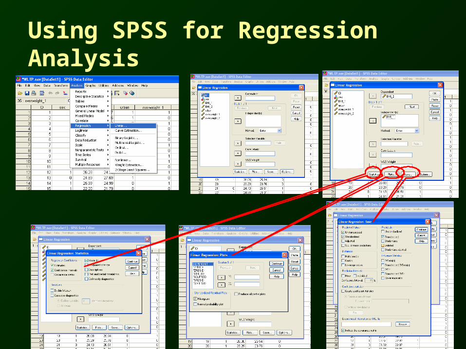
Using SPSS for Regression Analysis

SPSS Output
Model Summaryb
.657a .432 .431 1.47943Model1
R R SquareAdjustedR Square
Std. Error ofthe Estimate
Predictors: (Constant), BMI_1a.
Dependent Variable: BMI_2b.
ANOVAb
1660.355 1 1660.355 758.598 .000a
2184.337 998 2.189
3844.691 999
Regression
Residual
Total
Model1
Sum ofSquares df Mean Square F Sig.
Predictors: (Constant), BMI_1a.
Dependent Variable: BMI_2b.
Coefficientsa
-1.015 .893 -1.137 .256 -2.766 .737
1.024 .037 .657 27.543 .000 .951 1.097
(Constant)
BMI_1
Model1
B Std. Error
UnstandardizedCoefficients
Beta
StandardizedCoefficients
t Sig. Lower Bound Upper Bound
95% Confidence Interval for B
Dependent Variable: BMI_2a.
Residuals Statisticsa
19.3296 27.6322 23.5340 1.28919 1000
-4.23809 4.74759 .00000 1.47869 1000
-3.261 3.179 .000 1.000 1000
-2.865 3.209 .000 .999 1000
Predicted Value
Residual
Std. Predicted Value
Std. Residual
Minimum Maximum Mean Std. Deviation N
Dependent Variable: BMI_2a.

SPSS Output (cont.)

Using SPSS for OLS Test

SPSS Output (OLS Test)