using stressor-response relationships to derive … by... · 2018-04-18 · using stressor-response...
TRANSCRIPT

Office of Water EPA-820-S-10-001
Mail code 4304T November 2010
_____________________________________________________
Using Stressor-response Relationships to Derive Numeric Nutrient Criteria
Office of Science and Technology
Office of Water
U.S. Environmental Protection Agency
Washington, DC
Exhibit 11 (AR M.4)

ii
Disclaimer
This document provides technical guidance to States, authorized Tribes, and other authorized jurisdictions to develop water quality criteria and water quality standards under the Clean Water Act (CWA) to protect against the adverse effects of nutrient over-enrichment. Under the CWA, States and authorized Tribes are to establish water quality criteria to protect designated uses. State and Tribal decision-makers retain the discretion to adopt approaches on a case-by-case basis that differ from this guidance when appropriate. While this document presents methods to strengthen the scientific foundation for developing nutrient criteria, it does not substitute for the CWA or US EPA regulations; nor is it a regulation itself. Thus it cannot impose legally binding requirements on US EPA, States, authorized Tribes, or the regulated community, and it might not apply to a particular situation or circumstance. The US EPA may change this guidance in the future.
Exhibit 11 (AR M.4)

iii
Table of Contents
Table of Contents ................................................................................................................ iii
List of Figures ....................................................................................................................... v
Executive Summary ............................................................................................................. ix
Authors, Contributors, and Reviewers ............................................................................... xi
1 Introduction ................................................................................................................ 1
1.1 Overview of numeric criteria derivation approaches ......................................... 2
1.2 Relationship to other US EPA guidance .............................................................. 3
1.3 Document organization ...................................................................................... 4
2 Develop conceptual models ....................................................................................... 5
2.1 Lake conceptual models ..................................................................................... 6
2.2 Stream conceptual models ............................................................................... 10
3 Assemble and explore data ....................................................................................... 15
3.1 Select variables ................................................................................................. 15
3.2 Assemble the dataset ....................................................................................... 18
3.2.1 Data sources .............................................................................................. 18
3.2.2 Metadata ................................................................................................... 18
3.3 Summarize and visualize the dataset ............................................................... 19
3.3.1 Data distributions...................................................................................... 19
3.3.2 Bivariate summary and visualization methods ......................................... 23
3.3.3 Multivariate visualization methods .......................................................... 26
3.3.4 Mapping data ............................................................................................ 29
3.3.5 Data issues ................................................................................................ 30
4 Analyze data .............................................................................................................. 32
4.1 Simple linear regression .................................................................................... 32
4.1.1 Example data set ....................................................................................... 33
4.1.2 Simple linear regression assumptions ...................................................... 34
4.1.3 Deriving candidate criteria from stressor-response relationships ........... 37
4.1.4 Estimating prediction intervals by projection........................................... 46
4.2 Extensions of simple linear regression ............................................................. 49
Exhibit 11 (AR M.4)

iv
4.2.1 Multiple linear regression ......................................................................... 49
4.2.2 Quantile regression ................................................................................... 51
4.2.3 Nonparametric regression curves ............................................................. 52
4.2.4 Nonparametric changepoint analysis ....................................................... 53
4.3 Classifying data ................................................................................................. 55
4.3.1 Selecting classification variables ............................................................... 56
4.3.2 Statistical approaches for classification .................................................... 57
4.3.3 Finalizing a classification scheme ............................................................. 64
5 Evaluate and document analysis .............................................................................. 65
5.1 Evaluate model accuracy .................................................................................. 65
5.2 Evaluate model precision .................................................................................. 67
5.3 Consider implementation issues ....................................................................... 70
5.4 Document analyses ........................................................................................... 71
6 References ................................................................................................................ 72
Exhibit 11 (AR M.4)

v
List of Figures
Figure 2-1. Conceptual model diagram for lakes. See text for explanations for shapes and symbols. ..................................................................................................................... 10
Figure 2-2. Conceptual model diagram for streams. See text for explanation of shapes and symbols. ..................................................................................................................... 13
Figure 3-1. Example of variable selection to "block" an alternate pathway. Blocked pathway shown in as heavy arrows. Filled gray shapes show the stressor and response variables that are being modeled. Close up of lake conceptual model diagram shown in Figure 2-1. ......................................................................................................................... 15
Figure 3-2. Examples of histograms from EMAP-West Streams Survey for log-transformed TN and TP. Units in µg/L. ............................................................................ 20
Figure 3-3. Example boxplots from EMAP-West Streams Survey data for TN (left plot) and total taxon richness (right plot). Variable distributions within different ecoregions shown. MT : Mountains, PL: Plains, XE: Xeric. ................................................................. 21
Figure 3-4. Example cumulative distribution functions for TN across different ecoregions. Same data as shown in Figure 3-3. MT: Mountains, PL: Plains, XE: Xeric. ...................... 22
Figure 3-5. Quantile-quantile plots comparing TN (left plot) and log(TN) (right plot) values from EMAP-West to normal distributions. Solid line is drawn through the 1st and 3rd quartiles (shown as filled black circles) to help visualize the degree to which samples fall on a straight line. Units are µg/L (left plot) and log-transformed µg/L (right plot). .. 23
Figure 3-6. Scatter plot of TN versus a multimetric macroinvertebrate index of stream biological condition (MMI) from the EMAP-West Stream Survey in North and South Dakota, Wyoming, and Montana. ..................................................................................... 25
Figure 3-7. Scatter plot matrix of EMAP-West Streams Survey TN and TP (as log-transformed variables) against measures of grazing intensity in the watershed, and percent sand/fine substrates. Units are µg/L for TN and TP. Grazing intensity quantified as a unitless index score. .................................................................................................. 25
Figure 3-8. Example plots for conditional probability analysis for EMAP Northeast Lakes Survey data for chl a as response variable (threshold at 15 µg/L) and potential stressor variables TP and TN. .......................................................................................................... 26
Figure 3-9. Illustrative example of principle components analysis for two variables. Arrows labeled as PC1 and PC2 show the first and second principle components, respectively. ...................................................................................................................... 27
Figure 3-10. Example coplot showing the relationship between TN and MMI for different levels of bedded sediment. Dark orange bar at the top of each panel indicates the range of bedded sediment values included in that panel. Panels are numbered sequentially from low to high levels of bedded sediment. Bedded sediment quantified as percent sand/fines in the substrate. .............................................................................................. 29
Exhibit 11 (AR M.4)
vi
Figure 3-11. Map of TN data from EMAP-West Stream survey in North and South Dakota, Montana, and Wyoming. Symbol size is proportional to log TN concentration. 30
Figure 4-1. Total nitrogen (TN) versus chlorophyll a (chl a) in one lake collected during March-August over 10 years. Solid line: simple linear regression fit. ............................. 34
Figure 4-2. Quantile-quantile plot comparing residuals from the relationship shown in Figure 4-1 with a normal distribution. Solid line is drawn through the 1st and 3rd quartiles to help visualize the data. .................................................................................. 35
Figure 4-3. Residuals from regression fit shown in Figure 4-1 plotted versus predicted values. ............................................................................................................................... 36
Figure 4-4. Total nitrogen (TN) versus chl a in one lake collected during March-August over 10 years. Solid line: linear regression fit. Dashed lines: upper and lower 90th prediction intervals. Red horizontal line: chl a = 20 µg/L. Note that upper prediction interval has been extended beyond the range of the data to estimate the point at which it intersects the chl a threshold. Arrows indicate candidate criteria associated with different prediction intervals and the mean relationship. See text for details. .............. 39
Figure 4-5. Total nitrogen (TN) versus chl a in one lake collected during March-August over 10 years. Solid line: linear regression fit. Dashed lines: upper and lower 90th confidence intervals. ......................................................................................................... 40
Figure 4-6. Seasonally averaged TN versus chl a from March-August. Same data as shown in Figure 4-4. Solid line: linear regression fit. Dashed lines: upper and lower 90th prediction intervals. Red horizontal line: chl a = 20 µg/L. Arrows indicate candidate criterion values associated with different prediction intervals and the mean relationship (see text for details). Note that upper prediction interval has been extended beyond the range of the data to estimate the point at which it intersects the chl a threshold. ........ 41
Figure 4-7. Seasonally averaged TN versus chl a. Solid line: linear regression fit. Dashed lines: upper and lower 90th confidence intervals. ........................................................... 41
Figure 4-8. Annual average TN versus chl a in several similar lakes. Different symbols indicate different lakes. Lines indicate linear regression fits for TN-chl a relationship within each lake. Arrows indicate range of criteria associated with different lakes. ..... 42
Figure 4-9. Estimated slopes for TN versus chl a relationships in each of the five lakes shown in Figure 4-8. Vertical bars show 90% confidence intervals on estimated slopes............................................................................................................................................ 42
Figure 4-10. Upper prediction intervals for TN-chl a relationships in several similar lakes. Dashed lines show the upper 90% prediction intervals. Different symbols indicate different lakes. .................................................................................................................. 44
Figure 4-11. Synopic data set simulated by selecting 2 annual average values from each lake (shown as filled black circles). Open gray circles show all of the available seasonally averaged data to facilitate comparison with previous examples. Solid line shows linear
Exhibit 11 (AR M.4)

vii
regression fit to the synoptic data (filled black circles) and dashed lines show 90% prediction intervals. .......................................................................................................... 45
Figure 4-12. Projecting chl a values to a candidate criterion value. Arrows show the projection of sample values using estimated stressor-response relationship to a criterion value of TN = 1.1 mg/L. Projections are only calculated for samples in which TN concentration exceeds the candidate criterion value. ..................................................... 46
Figure 4-13. Example of using stressor-response relationship to predict chl a concentrations at a candidate criterion value. Arrows indicate the projection from current TN concentrations to the candidate criterion concentration. Two samples selected from each of five lakes (see Figure 4-11). Candidate criterion value of TN = 1.1 mg/L is shown as a vertical line. ....................................................................................... 48
Figure 4-14. Cumulative distribution frequencies of chl a values. Original distribution shown as open circles, and predicted distribution for a criterion value of TN = 1.1 mg/L shown as filled circles. ...................................................................................................... 49
Figure 4-15. Modeled relationship between TP, TN, and chl a. Plotted circles indicate combinations of TN and TP values observed in the data, and contour lines indicate modeled mean chl a concentrations (µg/L) associated with particular combinations of TN and TP. ......................................................................................................................... 50
Figure 4-16. Example of quantile regression. Same data as shown in Figure 4-1. Solid black lines are the 5th and 95th percentiles. Red horizontal line shows the response threshold of chl a = 20 µg/L. ............................................................................................. 51
Figure 4-17. Quantile regression with confidence limits. Solid black line is the estimated 95th percentile, dashed lines are the 95% confidence limits on position of the estimated quantile. ............................................................................................................................ 52
Figure 4-18. Example of nonparametric regression curve. TP versus chl a in one lake. Mean relationship estimated with a penalized regression spline. Solid line: estimated mean relationship. Dashed lines: 95% prediction intervals. ........................................... 53
Figure 4-19. Illustrative example of changepoint analysis for a stressor (X) and a response (Y). Solid line shows modeled response, with a step increase at X = 0.25. Vertical dashed lines show the 95% confidence intervals about the changepoint calculated from bootstrap resampling. ............................................................................ 55
Figure 4-20. Seasonally averaged TN versus chl a in example data. ................................ 58
Figure 4-21. Example of a simple classification by lake color. Black vertical lines indicate breakpoints between successive classes. Histogram indicates number of lakes observed at each color...................................................................................................................... 58
Figure 4-22. SLR estimates of relationship between TN and chl a in simple classes based on lake color. Classes are numbered sequentially from lowest to highest lake color. Dark orange bar at the top of each panel shows the range of color values included
Exhibit 11 (AR M.4)

viii
within each panel. Also see Figure 4-21 for ranges of lake colors included in each class............................................................................................................................................ 59
Figure 4-23. Simple classification approach for two variables. Black lines indicate possible thresholds between different classes. ................................................................ 60
Figure 4-24. Example of agglomerative clustering. Left plot: example of dendrogram using a small subset of the example lake data set. A horizontal line segment on the dendrogram indicates the Euclidean distance between the two branches below that segment. Right plot: Values of log color and log conductivity that correspond with sites shown in the dendrogram. Circles and squares around different letters indicate different classes. ............................................................................................................... 61
Figure 4-25. Classes specified with agglomerative clustering algorithm. Classes are numbered for later reference. Same data as shown in Figure 4-23. ............................... 62
Figure 4-26. Example of classification by propensity score. Same data as shown in Figure 4-23. Classes are numbered for later reference. .............................................................. 63
Figure 5-1. Stressor-response relationships computed within propensity score classes. Propensity score classes defined in Figure 4-26. Filled circles indicate samples from the single lake shown in Figure 4-6. Dashed lines indicate 90% prediction intervals. .......... 67
Figure 5-2. Illustration of range of chl a values associated with a selected criterion. Same data as Figure 4-8. Arrow B indicates TN criterion based on the least sensitive lake. Dashed arrow indicates prediction of mean chl a concentration at the most sensitive lake for this criterion value. ............................................................................... 68
Figure 5-3. Refinement of classification of sites for Class 1 (see Figure 5-1). Filled circles indicate sites that are excluded by classification refinement. Solid line and dashed lines indicate SLR fit and 90% prediction intervals for remaining sites in class. ....................... 69
Exhibit 11 (AR M.4)

ix
Executive Summary
For over a decade, the U.S. Environmental Protection Agency (EPA) has recognized the importance of developing numeric water quality criteria to protect the designated uses of waterbodies from nutrient enrichment that is associated with broadly occurring levels of nitrogen/phosphorus pollution. EPA recommends three types of scientifically defensible empirical approaches for setting numeric criteria to address nitrogen/phosphorus pollution (US EPA 2000a and 2000b): reference condition approaches, mechanistic modeling, and stressor-response analysis. This document elaborates on the third of these three approaches by providing a four-step process for estimating and interpreting stressor-response relationships for deriving numeric criteria to address nitrogen/phosphorus pollution.
In the first step, conceptual models representing known relationships between nitrogen (N) and phosphorus (P) concentrations, biological responses, and attainment of designated uses are developed for the study area. To facilitate developing these models, the guidance document provides detailed conceptual models for lakes and streams that can be modified according to the characteristics of the local study area.
In the second step, data are assembled and initial exploratory analyses are performed. Variables are selected during this step that represent different concepts shown on the conceptual model, including variables that represent N and P concentrations, variables that represent responses that can be directly linked with designated uses, and variables that can potentially confound estimates of stressor-response relationships. After selecting variables and assembling data, these data are explored to provide insights into how different variables are distributed and how groups of variables covary with one another. These exploratory analyses inform subsequent development of formal statistical models.
In the third step, stressor-response relationships are estimated between N and P concentrations and the selected response variables, and criteria are derived from these relationships. The guidance document presents an analysis approach that emphasizes classification, to maximize the accuracy and precision of estimated stressor-response relationships, and simple linear regression, to provide stressor-response relationships that can be most easily interpreted for criteria derivation. Methods for interpreting simple linear regression models in terms of predicting the probability of different outcomes are discussed in the context of criteria derivation.
In the final step, the accuracy and precision of estimated stressor-response relationships are evaluated and the analyses documented. The accuracy of estimated relationships is evaluated with regard to the possible influence of known confounding variables as identified by the conceptual model or by exploratory data analysis. The required precision of estimated relationships depends strongly on the relevant management decisions, and so, evaluating precision is discussed in this context.
Exhibit 11 (AR M.4)

x
Numeric criteria are important for protecting our nation’s waterbodies from the well-established negative effects of nitrogen/phosphorus pollution. These criteria can be developed using a variety of approaches, including stressor-response relationships, and this guidance describes a specific process for conducting such analyses. The process described will support states, territories, and authorized tribes in incorporating stressor-response relationships into their numeric criteria development programs and further the goal of reducing nitrogen/phosphorus pollution nationwide.
Exhibit 11 (AR M.4)

xi
Authors, Contributors, and Reviewers
AUTHORS
Lester L. Yuan, Dana A. Thomas Office of Science and Technology Office of Water U. S. Environmental Protection Agency Washington DC John F. Paul National Health and Environmental Effects Research Laboratory Office of Research and Development U. S. Environmental Protection Agency Research Triangle Park, NC Michael J. Paul, Melissa A. Kenney Center for Ecological Sciences, Tetra Tech, Inc. Owings Mills, MD
REVIEWERS
Internal EPA Reviewers
Mark Barath Region 3 Philadelphia, PA
Peter Leinenbach Region 10 Seattle, WA
Susan Cormier National Center for Environmental Assessment Office of Research and Development Cincinnati, OH
Dave Mount National Health and Environmental Effects Research Laboratory Office of Research and Development Duluth, MN
James Curtin Office of General Counsel Washington, DC
Susan B. Norton National Center for Environmental Assessment Office of Research and Development Washington, DC
Christopher Day Region 3 Philadelphia, PA
Barbara Pace Office of General Counsel Washington, DC
Exhibit 11 (AR M.4)

xii
David Farrar National Center for Environmental Assessment Office of Research and Development Cincinnati, OH
Margaret Passmore Region 3 Wheeling, WV
Terry Fleming Region 9 San Francisco, CA
Suesan Saucerman Region 9 San Francisco, CA
John Goodin Office of Wetlands, Oceans, and Watersheds Office of Water Washington, DC
Glenn Suter National Center for Environmental Assessment Office of Research and Development Cincinnati, OH
Treda Grayson Office of Wetlands, Oceans, and Watersheds Office of Water Washington, DC
Anett Trebitz National Health and Environmental Effects Research Laboratory Office of Research and Development Duluth, MN
Lareina Guenzel Region 8 Denver, CO
John Van Sickle National Health and Environmental Effects Research Laboratory Office of Research and Development Corvallis, OR
Michael Haire Office of Wetlands, Oceans, and Watersheds Office of Water Washington, DC
Danny Wiegand Office of Science Policy Office of Research and Development Washington, DC
Tina Laidlaw Region 8 Helena, MT
Izabela Wojtenko Region 2 New York, NY
Jim Latimer National Health and Environmental Effects Research Laboratory Office of Research and Development Narragansett, RI
Exhibit 11 (AR M.4)

xiii
External reviewers William H. Clements Dept. of Fish, Wildlife and Conservation Biology Colorado State University Fort Collins, CO Thomas J. Danielson Maine Department of Environmental Protection August, ME Charles P. Hawkins Dept. Watershed Sciences Utah State University Logan, UT Neil Kamman Vermont Department of Environmental Conservation Waterbury VT Ryan S. King Department of Biology Baylor University Waco, TX Song S. Qian Nicholas School Duke University Durham, NC Ecological Processes and Effects Committee EPA Science Advisory Board
Exhibit 11 (AR M.4)

1
1 Introduction
Under the Clean Water Act, states, territories, and authorized tribes are responsible for establishing water quality standards that specify designated uses for different waterbodies, establish criteria to protect those uses, and contain an anti-degradation provision to protect existing uses. Numeric criteria are an important element of water quality standards that provide a tool for managing the impacts of nitrogen/phosphorus pollution on waters of the United States. Natural background levels of nutrients, especially nitrogen (N) and phosphorus (P), are essential for balanced plant and microbial growth under natural concentrations; however, it is well-established that anthropogenic activities resulting in high concentrations of N and P in the water stimulates excessive plant and microbial growth. This excess growth produces deleterious physical, chemical, and biological responses in surface water and impairs designated uses in both receiving and downstream waterbodies (Vitousek et al. 1997, Carpenter et al. 1998, Smil 2000, Bennett et al. 2001, Reckhow et al. 2005). Nutrients are consistently among the top 3 causes of use impairment nationwide (see http://iaspub.epa.gov/waters10/attains_nation_cy.control#causes), and there is ongoing interest in numeric criteria to address these impairments.
Criteria derivation methods developed by the US EPA for the toxic effects of chemical pollutants (US EPA 1985) have limited applicability to nutrients because the effects of nitrogen/phosphorus pollution, while linked to widespread and significant aquatic degradation, occur through a series of intermediate steps that are difficult to replicate in simple laboratory studies (Odum et al. 1979). In some cases, N and P concentrations have been experimentally manipulated (e.g., Pan et al. 2000, Cross et al. 2006), but in general, numeric criteria derivation for N and P often relies on analyses of observational data collected in the field. To assist states and tribes with assembling and analyzing appropriate data, the US EPA has released a series of peer-reviewed technical guidance documents for developing nutrient criteria for different waterbodies (rivers and streams, US EPA 2000a; lakes and reservoirs, US EPA 2000b; estuarine and coastal waters, US EPA 2001; and wetlands, US EPA 2008). These documents describe three types of empirical analyses that can be used to derive numeric criteria: (1) the reference condition approach, (2) mechanistic modeling, and (3) stressor-response analysis (US EPA 2000a, 2000b).
This document supplements existing nutrient criteria guidance (USEPA 2000a, 2000b, 2001, and 2008) by providing detailed approaches for estimating and interpreting stressor-response relationships for developing numeric criteria to address nitrogen/phosphorus pollution. The intended audiences include state, tribal, local, and regional scientists who collect and analyze field data in support of criteria derivation. Other stakeholders may find this document useful as well. The guidance assumes readers have graduate-level training or experience in both aquatic sciences and statistics.
Exhibit 11 (AR M.4)

2
1.1 Overview of numeric criteria derivation approaches
The three types of empirical analyses provide distinctly different, independently and scientifically defensible, approaches for deriving numeric criteria from field data. Data requirements differ for each of these approaches. The reference condition approach derives candidate criteria from observations collected in reference waterbodies. Reference waterbodies represent least disturbed and/or minimally disturbed conditions within a region (Stoddard et al. 2006a) that support designated uses (US EPA 2000a). Therefore, the range of conditions observed within reference waterbodies provides appropriate values upon which criteria can be based. Criteria for a particular variable (e.g., total phosphorus or total nitrogen) are derived by compiling measurements of that variable from reference waterbodies and selecting a representative value from the resulting distribution. The reference condition approach requires the ability to define and identify reference waterbodies, and relies on the availability of sufficient data from these reference waterbodies to characterize the distributions of different nutrient variables.
The mechanistic modeling approach represents ecological systems using equations that represent ecological processes and parameters for these equations that can be calibrated empirically from site-specific data. These models can then be used to predict changes in the system, given changes in N and P concentrations. Mechanistic models have been developed for a wide range of water quality processes that are described in existing nutrient criteria guidance documents (e.g., US EPA 2000a, 2000b), and in greater detail in water quality modeling textbooks (e.g., Chapra 1997). Guidance on the development, evaluation, and application of mechanistic models is also available (US EPA 2009). Some of these models can be used to account for site-specific effects of N and P enrichment and can mechanistically link changes in concentration to impairment of designated uses. The mechanistic modeling approach requires sufficient data to identify the appropriate equations for characterizing a waterbody or group of waterbodies and sufficient data to calibrate parameters in these equations.
Empirical stressor-response modeling is used when data are available to accurately estimate a relationship between N and P concentrations and a response measure that is directly or indirectly related to a designated use of the waterbody (e.g., a biological index or recreational use measure). Then, N and P concentrations that are protective of designated uses can be derived from the estimated relationship (US EPA 2000a, 2000b, and 2008). These data requirements usually extend beyond measurements of concentrations and responses, and include measurements of other environmental factors that potentially can confound the estimated relationships (see Section 3.1). As noted earlier, the stressor-response approach is the focus of the current document.
Each of these three analytical approaches is appropriate for deriving scientifically defensible numeric criteria to address the effects of nitrogen/phosphorus pollution when applied with consideration of method-specific data needs and available data. In addition to these empirical approaches, consideration of established (e.g., published)
Exhibit 11 (AR M.4)

3
nutrient response thresholds is also an acceptable approach for deriving criteria (US EPA 2000a).
1.2 Relationship to other US EPA guidance
The US EPA has developed a number of guidance documents to support development of numeric criteria (US EPA 2000a, 2000b, 2001, 2008). While these documents provide detailed information pertaining to nutrient criteria derivation for different types of waterbodies, they vary in their coverage of stressor-response relationship modeling. The lake guidance, for example, provides detailed coverage of traditional nutrient-chlorophyll a models that have been a critical element of modern lake water quality management (US EPA 2000b). In contrast, the streams and rivers guidance provides an overall framework for nutrient criteria derivation and implementation and extensive detail regarding reference condition approaches, but provides less detail on estimating stressor-response relationship models (US EPA 2000a). This current document strengthens existing nutrient criteria guidance documents by providing greater detail on estimating stressor-response relationship models and on incorporating these models into the numeric criteria derivation process.
The information provided in this document has much in common with practices that are recommended in US EPA’s Ecological Risk Assessment Guidelines (US EPA 1998). More specifically, the current document describes activities that occur during the problem formulation and data analysis stages of an ecological risk assessment. During problem formulation, one develops a conceptual model that describes preliminary hypotheses regarding why ecological effects have occurred, or may occur, from human activities. Then, one selects assessment endpoints and develops an analysis plan. In previous nutrient guidance documents and in this document, conceptual models are provided that describe linkages between nitrogen/phosphorus pollution, biological effects, and designated uses (Section 2). Similarly, selection of assessment endpoints and measures of effects are discussed in Section 3.1. However, the majority of the material covered in this current document is comparable to the analysis phase of ecological risk assessment, in which stressor-response relationships are estimated.
This document also has much in common with existing guidance on the use of environmental models (US EPA 2009), as any stressor-response relationship can be regarded as one particular type of environmental model. However, the US EPA environmental modeling document (2009) primarily emphasizes mechanistic models as defined above, in contrast to the stressor-response models described in the current document.
Relationships with other related US EPA guidance covering topics such as data quality (US EPA 2006) and stressor identification (US EPA 2010) are addressed in the appropriate sections of this document (i.e., Section 3.2.2, where data quality is discussed, and Section 2, where stressor identification is discussed in the context of developing conceptual models).
Exhibit 11 (AR M.4)

4
1.3 Document organization
Four steps are involved when stressor-response relationships are used to derive numeric nutrient criteria. First, conceptual models are developed to represent known relationships between changes in N and P concentrations, biological effects, and attainment of designated uses (Section 2). These conceptual models not only provide a means of communicating the current state of knowledge regarding the effects of N and P in aquatic systems, but also provide an important tool for guiding subsequent analyses. Second, variables are selected for analysis, data are assembled, and characteristics of these data explored (Section 3). Third, data are analyzed to estimate stressor-response relationships depicted in the conceptual models (Section 4). In this guidance, a three-stage approach to analysis is recommended, in which waterbodies are first classified, stressor-response relationships are estimated within each class, and criteria are derived from the estimated relationships. Fourth, analyses are reviewed, evaluated and documented (Section 5). These steps are presented sequentially but substantial iteration within and across different steps is expected when deriving candidate criteria.
Throughout the document, examples are provided that have been selected specifically to illustrate different statistical analyses and to illustrate how to interpret the results of these analyses to derive candidate numeric criteria. These analyses can be applied to different types of waterbodies, including freshwater, wetlands, estuarine, and marine systems if sufficient data are available on causal variables, response variables, and confounding factors. The following sections are not intended to provide exhaustive coverage on how to complete individual analyses, and interested readers should consult qualified statisticians or appropriate literature for additional technical information.
Exhibit 11 (AR M.4)

5
2 Develop conceptual models
A conceptual model diagram is a visual representation of relationships among human activities, stressors such as nitrogen/phosphorus pollution, biotic responses, and designated uses in aquatic systems. Conceptual model diagrams and their accompanying narrative descriptions (together, referred to as conceptual models) are useful tools for stressor-response analysis for two reasons: they depict accepted scientific knowledge, and they help guide model development.
First, the diagrams depict accepted scientific knowledge regarding the effects of nitrogen/phosphorus pollution in surface waters. The causal pathways that lead from human activities to excess N and P to impacts on designated uses in lakes and streams are well established in the scientific literature (e.g., streams: Stockner and Shortreed 1976, Stockner and Shortreed 1978, Elwood et al. 1981, Horner et al. 1983, Bothwell 1985, Peterson et al. 1985, Moss et al. 1989, Dodds and Gudder 1992, Rosemond et al. 1993, Bowling and Baker 1996, Bourassa and Cattaneo 1998, Francoeur 2001, Biggs 2000, Rosemond et al. 2001, Rosemond et al. 2002, Slavik et al. 2004, Cross et al. 2006, Mulholland and Webster 2010; lakes: Vollenweider 1968, NAS 1969, Schindler et al. 1973, Schindler 1974, Vollenweider 1976, Carlson 1977, Paerl 1988, Elser et al. 1990, Smith et al. 1999, Downing et al. 2001, Smith et al. 2006, Elser et al. 2007). To assist the reader in developing their own models, conceptual models are provided in this section that describe the known causal pathways connecting nitrogen/phosphorus pollution to impacts on the designated use in lakes and streams.
Second, conceptual models help guide the development of stressor-response models. Conceptual models identify relationships that can be modeled with statistical analyses and help analysts identify variables, in addition to the main nutrient and response variables, that should be considered during analysis. More specifically, conceptual model diagrams provide a graphical means of identifying potentially confounding variables, which are defined as variables that can influence estimates of the stressor-response relationships (see Section 3.1). This emphasis on identifying potentially confounding variables dictates that the diagrams include other pathways linking human activities to biological responses and designated uses, which is a slightly different emphasis than conceptual models developed for other purposes. Hence, the model diagrams provided here more comprehensively describe both nutrient related and non-nutrient pathways linking human activities to designated uses. However, all relevant pathways cannot be included in the model diagrams provided here, and it is expected that analysts would modify these diagrams by adding or removing concepts and pathways based on the details of a particular location or system. More complete conceptual model diagrams can be found at http://www.epa.gov/caddis, where the development of conceptual models is presented as key step in stressor identification.
Each conceptual model diagram is presented as a series of linked shapes, each representing a distinct concept. Different shapes represent different types of concepts: octagons represent human activities, rectangles represent primary stressors and
Exhibit 11 (AR M.4)

6
responses, pentagons represent environmental factors that can modify relationships between primary stressors and responses, and ovals represent designated uses. Within each shape, an arrow pointed up (↑) indicates an increase, an arrow pointed down (↓) indicates a decrease, and a delta symbol (Δ) indicates a change in the given concept, either through time or when compared with a reference site. Arrows leading from one shape to another indicate known causal relationships, which can be interpreted as the originating shape causing the indicated change in the shape to which it points.
Separate conceptual model diagrams are provided for lakes and streams. A number of pathways are similar in both of these systems; however, there are some effects of nitrogen/phosphorus pollution that are unique to lake or stream systems. Also, the relative importance of pathways can differ between these two systems. To aid in comparison, the models are presented in a similar fashion. Each model diagram depicts anthropogenic activities that both generate and affect the transport of pollutants at the top of the diagram. It then indicates key intermediate steps linking anthropogenic activities to increased N and P concentrations and other stressors. These pathways then lead to the proximate stressors that ultimately affect designated use responses. Interacting or confounding factors that modify or influence the effect of stressors or steps along the stressor-response pathway are also depicted.
In the context of these models and in this document, the term “stressor” refers to any factor that causes adverse effects in organisms of interest. Stressors differ in the degree to which they directly affect organisms. For example, toxic chemicals such as pesticides can directly affect fish, whereas increased N and P concentrations may affect fish through several intermediate steps. The term stressor is used generically here to include factors at all steps along a particular pathway.
The models provided in this section provide a brief overview of the causal pathways linking different human activities to impairment of designated uses in streams and lakes. These models emphasize pathways leading to and from nitrogen/phosphorus pollution, but as noted earlier, other potential pathways are included to help identify variables that may confound estimated stressor-response relationships (see Section 3.1). Models provided in this section should be adapted to activities and pathways that are relevant to a particular study area.
2.1 Lake conceptual models
One of the most important processes in the lake conceptual model is eutrophication, the process whereby increased N and P concentrations cause increases in the system’s primary productivity (Novotny 2003). When this document refers to eutrophication, it refers specifically to cultural eutrophication, whereby human activities alter the rates of N and P input, export, and cycling, accelerating increases in productivity and causing a
Exhibit 11 (AR M.4)

7
range of water quality problems (Carlson 1977, Chapra 1997, Smith et al. 1999, Smith et al. 2006). The term “nutrient enrichment” is also used to differentiate pathways considered in these conceptual models from the toxic effects of some nutrient forms (e.g., ammonia and nitrate) that can occur at higher concentrations.
The lake conceptual model diagram presents pathways linking human activities to increased N and P loading, increased N and P concentrations, and other stressors that affect designated uses (Figure 2-1). For lakes, the most important pathway for deriving numeric criteria links increased N and P concentrations, coupled with light and temperature, to an increase in primary productivity (Lee et al. 1978, Smith 1998). This increased primary production increases organic carbon, which fuels increased respiration, which, in turn, reduces dissolved oxygen concentration. Decreased dissolved oxygen then influences the health and species composition of aquatic life. Although this primary eutrophication pathway is expected in most lake systems, its importance, magnitude, and effect can vary across regions and sites within a region.
Human activities that increase the loading and subsequent in-lake concentrations of N and P are categorized generally as point sources, urban nonpoint sources, and agricultural nonpoint sources. Point sources include any discharges that can be associated with discrete locations (e.g., publicly owned treatment works). Point sources of nutrients include municipal wastewater, industrial wastewater, and confined animal feeding operations. These wastewaters differ in their sources and level of treatment, and therefore differ in the magnitude and forms of N and P that they convey into lakes (Dunne and Leopold 1978). Point sources can also introduce toxic pollutants to lakes, but the specific characteristics of these toxicants also differ with the waste source and level of treatment.
Nonpoint sources are human activities on the landscape that cannot be associated with a single discharge location. Urban nonpoint source runoff includes fertilizers, animal feces, and other chemicals and causes elevated lake N and P concentrations (Carpenter et al. 1998). Erosion of nutrient-enriched soils is also common in urban areas and contributes to both elevated N and P concentrations and increased suspended sediment concentrations. Metals, pesticides, and other toxicants from a variety of different anthropogenic activities in urban areas are also observed in urban runoff.
Agricultural activities generally produce nonpoint source pollutants, with the exception of discrete discharges from confined animal feeding operations, which are included with point sources in this model. Relevant agricultural activities that increase N and P loading in lakes include fertilizer and manure applications. Erosion from land disturbance associated with agricultural activities can also cause increased nutrient loads when N and P, bound to watershed soils, are mobilized (Dunne and Leopold 1978, Carpenter et al. 1998). These activities can also increase suspended sediment, a stressor that frequently co-occurs with nutrients. Many of these same activities can also introduce toxicants (e.g., pesticides) that affect aquatic life.
In addition to these human influenced inputs, underlying geology and natural vegetation in some systems influences baseline N and P concentrations. For example, some soils
Exhibit 11 (AR M.4)

8
and bedrock have a naturally high N or P content, which contribute to nutrient loading (Omernik et al. 2000). Similarly, natural organic debris can contribute to nitrogen loading.
Regardless of their source, N and P are present in three main forms: dissolved organic N and P, dissolved inorganic N and P, and particulate N and P (Chapra 1997). These compounds frequently cycle between forms, transforming and reacting between dissolved and particulate fractions. Only dissolved organic and inorganic forms are taken up by microbes and primary producers, and this uptake capacity and rate varies among taxa and environmental conditions.
For P, soluble reactive phosphorus (e.g., PO4) is the form most readily available to plants and algae (Correll 1998). Although soluble PO4 concentration can be measured directly, it is taken up by plants or converted to other forms quickly in the environment, and measurements of soluble PO4 may not provide an accurate indication of available P. Therefore, total P (TP) is commonly measured and used as an indicator of the amount of P available to the system. Estimates of P loading have also been combined with lake retention time and P settling rates to model observed chl a concentrations (Vollenweider 1976).
For N, inorganic N in the forms of ammonia (NH3) and nitrate (NO3) are preferred by plants and algae. Like PO4, it is often difficult to measure NH3 and NO3 frequently enough in most state sampling programs to capture nutrient-plant dynamics. Thus, total N (TN) is commonly used to represent the amount of N in the system and its relationship to primary production.
In addition to N and P additions from point and nonpoint sources, concentrations can be affected by several lake characteristics including retention time, lake depth, and stratification (Vollenweider 1968, Dake and Harleman 1969, Gorham and Boyce 1989). Retention time, or residence time, is the amount of time that an average water molecule or substance particle would remain in the lake system. The smaller the residence time, the faster the flushing rate and the faster nutrients leave the system. Lake depth affects internal nutrient cycling, or internal nutrient load, in a lake. Shallower lakes have greater potential nutrient cycling because N and P released from bottom sediments or concentrated in lower depths are more easily mixed with the top of the water column. This process is exacerbated by anoxia at depth, which enhances phosphorus remineralization. Stratification is the physical process whereby a lake separates into distinct layers of different water densities. In a stratified lake, the top layer is known as the epilimnion; the middle layer, the metalimnion; and bottom layer, the hypolimnion. The thermocline is a layer where water temperature and density change most rapidly, separating the epilimnion from the hypolimnion. Cold, temperate lake systems are usually stratified except for turnover events in the spring and fall, when the system becomes completely mixed. In regions without winter ice cover, turnover may occur throughout the winter and only stratify in the summer. In the southern US, shallow lakes may alternately mix and stratify. While a lake is stratified, nutrients cycle within the epilimnion and exchange with other layers occurs through settling, internal
Exhibit 11 (AR M.4)

9
mixing, and diffusion (Chapra 1997). Also, under stratified conditions, dissolved oxygen in the hypolimnion can be depleted leading to anoxic conditions.
These lake characteristics are inter-related. Lake depth affects retention time and lake temperature. In general, a deeper lake has a longer retention time and a lower average temperature (as measured by a depth integrated sample). Stratification is also affected by lake depth, fetch, and temperature (Dake and Harleman 1969, Gorham and Boyce 1989). Stratification in deep lakes is predominantly affected by water temperature, which controls water density, the main factor in stratification. Fetch, the distance wind can travel unobstructed over the lake surface, affects 1) mixing within the epilimnion in stratified lakes, 2) timing of the fall or spring turnover (i.e., wind provides turbulence needed to initiate mixing of the layers), or 3) overall mixing in shallow, well-mixed systems.
One of the most important relationships in lakes with regard to nutrient criteria is the causal link among N and P, light, temperature, and primary productivity (Lee et al. 1978). Increased levels of N and P cause an increase in primary productivity (i.e., growth of phytoplankton and macrophytes). Both P and N can control phytoplankton growth in a lake. In many freshwater lake systems, P is recognized as the limiting nutrient (Vollenweider 1968, Vollenweider 1976, Reckhow 1979, Schindler et al. 2008, Correll 1998); however, research has demonstrated that N and co-limitation by N and P can be important in these systems (Smith 1982, Downing and McCauley 1992, Elser et al. 1990, Smith 1979). In addition to nutrients, light and temperature are essential to plant growth. Though the optimal light level or temperature varies for each species, in general, as light and temperature increases, phytoplankton growth also increases until some optimal level is reached.
Color and suspended sediments in a lake can change the light available for photosynthesis. In some systems, humic acids from dissolving plant matter or dissolved minerals change the water color from clear to tea colored, reducing available light. Similarly, increased suspended sediments, which can often co-occur with increased N and P, reduce light availability. Increased primary productivity itself increases organic and particulate matter and thus, also reduces light availability.
Increased primary productivity increased dissolved oxygen concentrations during daylight hours. However, increased primary productivity also increases respiration (i.e., consumption of O2) as increased abundances of macrophyte and phytoplankton themselves respire carbohydrates generated by photosynthesis to support growth and maintenance. The cycle of photosynthesis and respiration causes predictable diurnal cycles in dissolved oxygen concentrations. Increased primary production ultimately becomes detrital carbon, which increases the organic matter load and further fuels the respiration of microbial decomposers. Increased respiration consumes dissolved O2 in the water. Changes in primary productivity and decomposition rates also ultimately alter the food quantity in the system, by changing the amount of available detrital or primary production carbon available to consumers.
Exhibit 11 (AR M.4)
10
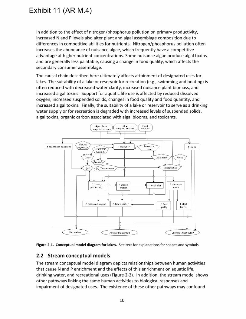
In addition to the effect of nitrogen/phosphorus pollution on primary productivity, increased N and P levels also alter plant and algal assemblage composition due to differences in competitive abilities for nutrients. Nitrogen/phosphorus pollution often increases the abundance of nuisance algae, which frequently have a competitive advantage at higher nutrient concentrations. Some nuisance algae produce algal toxins and are generally less palatable, causing a change in food quality, which affects the secondary consumer assemblage.
The causal chain described here ultimately affects attainment of designated uses for lakes. The suitability of a lake or reservoir for recreation (e.g., swimming and boating) is often reduced with decreased water clarity, increased nuisance plant biomass, and increased algal toxins. Support for aquatic life use is affected by reduced dissolved oxygen, increased suspended solids, changes in food quality and food quantity, and increased algal toxins. Finally, the suitability of a lake or reservoir to serve as a drinking water supply or for recreation is degraded with increased levels of suspended solids, algal toxins, organic carbon associated with algal blooms, and toxicants.
Figure 2-1. Conceptual model diagram for lakes. See text for explanations for shapes and symbols.
2.2 Stream conceptual models
The stream conceptual model diagram depicts relationships between human activities that cause N and P enrichment and the effects of this enrichment on aquatic life, drinking water, and recreational uses (Figure 2-2). In addition, the stream model shows other pathways linking the same human activities to biological responses and impairment of designated uses. The existence of these other pathways may confound
Exhibit 11 (AR M.4)

11
the relationships estimated among N and P concentrations, responses, and impairment of designated uses. Note also that the number of other pathways (and therefore, the number of possible confounding factors) increases with the number of steps between the causal and response variable. Therefore, many confounding variables must be considered when estimating the effects of nitrogen/phosphorus pollution on a measure of aquatic life in streams (e.g, a macroinvertebrate index). Conversely, relatively few confounding variables must be considered when estimating the effects of nitrogen/phosphorus pollution on primary productivity (see discussion regarding variable selection in Section 3.1). It is important to assess whether sufficient data are available to support the application of this particular methodology. If data are not available to control for the effects of stressors other than nitrogen and phosphorus in specific streams, it does not reduce the strength of the underlying well-established and documented cause-effect relationship referenced in this chapter. Because of the possible burden of acquiring the additional data that may be necessary to support this approach, readers may also want to consider relying on the additional approaches noted above, including the reference condition approach.
The sources of nitrogen/phosphorus pollution to streams (agricultural nonpoint sources, urban nonpoint sources, and point sources) are categorized in the same manner as for lakes. Similar to lakes, one of the more important pathways by which nutrient enrichment affects designated uses in streams is by increasing primary productivity. Increased N and P also alter the composition of the primary producer assemblage (Rosemond et al. 1993, Slavik et al 2004), including the amount and ratio of edible and non-edible forms, which alters herbivore assemblages (Feminella and Hawkins 1995, Hillebrand 2002). Food quantity may be increased by excess organic matter (from increased primary production), which also favors some consumers over others and changes the natural composition of taxa evolved to compete for natural amounts of different food types (Hawkins et al. 1982, Fuller et al. 1986, Wallace and Gurtz 1986). Excess primary production also alters physical habitat. For example, excess filamentous algae alters the normal physical habitat, interfering with movement, affecting visual predation, and blocking access to feeding and reproductive habitat for some organisms (Slavik et al 2004), while favoring others (Dudley et al. 1986).
The effect of nitrogen/phosphorus pollution on primary production is influenced by light availability and temperature. Light can limit primary production in flowing waters, especially in well-shaded headwater streams or large, turbid rivers (e.g., Fisher and Likens 1973, Vannote et al. 1980, Fuller et al. 1986). Terrestrial plants, stream color, suspended sediments, and morphological elements, such as stream incision and aspect, all influence light availability (Philips et al. 2000, Hill et al. 1995). Suspended sediments are composed of inorganic as well as organic material, including suspended algal material composed of either tychoplankton (detached benthic algae in the water column) or true phytoplankton. Therefore, excess primary production can also contribute to shading, but this phenomenon is limited to deeper rivers. Temperature is a main determinant of metabolic rates and influences rates of primary production and respiration.
Exhibit 11 (AR M.4)

12
Nitrogen/phosphorus pollution also increases microbial production (fungi and bacteria), increasing the rate at which these organisms decompose organic matter, an important food resource for other biota in streams (Gulis and Suberkropp 2003, Gulis et al. 2004). Increased decomposition rates alter the timing and the amount of organic matter available to higher trophic levels (Cross et al. 2006). It can also influence the availability and amount of coarse versus fine particulate organic matter, which influences aquatic consumer assemblages (Cummins and Klug 1979).
The combined effect of increased organic matter (from increased primary productivity) and increased microbial activity is an increase in heterotrophic respiration, which consumes dissolved oxygen (Allan and Castillo 2007). Dissolved oxygen availability is critical to invertebrate and vertebrate taxa, and different species vary in their requirements for dissolved oxygen. As a result, changes in oxygen concentrations alter aquatic communities (e.g., Miranda et al. 2000, Caraco et al. 2006). The magnitude of oxygen reduction and the duration of low oxygen conditions influence the extent of the impact. Anoxia and hypoxia vary across streams and even within streams, as some areas (e.g., back or slackwater areas) may become more stagnant and hypoxic than main channel flow (e.g., Miranda et al. 2000). In the main channel, slowly flowing waters may also not aerate quickly and dissolved oxygen concentrations may be low. Streams that are well aerated and shallow will generally experience less of an effect of reduced oxygen due to nutrient enrichment than poorly re-aerated, deeper streams (Allan and Castillo 2007).
Designated uses are affected by human activities via other pathways besides nitrogen/phosphorus pollution, and understanding these other pathways can help one design analyses to minimize the potential for other environmental factors to confound estimates of stressor-response relationships (see Section 3.1). For example, in addition to increasing N and P loads, urban nonpoint sources alter flow characteristics in streams. Increased amounts of impervious surfaces in urban areas reduce precipitation infiltration and increase surface runoff, which is manifested as increased flood frequencies and magnitudes. These altered flow characteristics increase stream scour, which reduces primary producer accrual, reduces carbon storage (food quantity), and degrades physical habitat quality by altering substrate stability and composition (Paul and Meyer 2001). Also, both urban and agricultural nonpoint sources often increase sediment and toxic loads to streams.
Recreational uses are principally affected when water clarity compromises swimming safety or when nuisance algal growth reduces desirability for swimming (Suplee et al. 2009). Water clarity is reduced when suspended material, including inorganic and organic sediments, are elevated. Inorganic sediments are another common stressor that co-occurs with nutrients, and suspended organic sediments can be caused by excess primary production. Reduced clarity affects light availability and the ability to identify submerged obstacles, affecting swimmer safety (WHO 2003). Reduced clarity also may influence fishing success for certain game species. Nuisance algal growth includes excess growth of periphyton, which can make stream substrates slippery and dangerous for wading and fishing. Nuisance growth also includes excess growth of
Exhibit 11 (AR M.4)

13
filamentous algae and macrophytes that entangle swimmers, reduce clarity for fishing, and reduce the general desirability for water contact.
Similarly, drinking water uses are also affected by nuisance algae and suspended sediments. Some nuisance algae produce compounds that produce toxins that pose direct health risks and affect taste and odor (WHO 2003). Increased suspended organic and inorganic sediments can increase treatment costs.
Nitrogen/phosphorus pollution generally does not typically exert direct adverse effects on higher trophic levels (e.g., fish and invertebrates). However, indirect effects of nutrient enrichment affects aquatic life at these higher trophic levels through a number of different pathways, including reduced physical habitat quality, decreased dissolved oxygen concentrations, alterations to food quantity and quality, and increased nuisance plant and algae growth that may increase algal toxins and reduce food quality.
Figure 2-2. Conceptual model diagram for streams. See text for explanation of shapes and symbols.
Other chemical pathways influenced by nitrogen/phosphorus pollution can affect aquatic life, but for simplicity, these pathways are not displayed in the conceptual model diagram. For example, in poorly buffered systems, high rates of metabolism during periods of excess respiration increase CO2 concentrations, which can reduce pH. Similarly, during periods of excess primary production, consumption of CO2 increases pH (Caraco et al. 2006). These fluctuations in pH can be stressful to aquatic organisms (Wetzel 2001). Fluctuations in dissolved oxygen concentration can also affect sediment
Exhibit 11 (AR M.4)

14
oxygen concentrations that influence redox potentials and, subsequently, biogeochemical reactions such as metal speciation, and therefore, the toxicity of different metals (Wetzel 2001).
Exhibit 11 (AR M.4)

15
3 Assemble and explore data
Exploratory data analysis (EDA) is an approach to examine and visualize data to understand likely relationships, indicate appropriate statistical modeling approaches, and assess the basis for statistical modeling assumptions (Tukey 1977). Prior to conducting EDA, one must select variables for analysis and assemble the data set. In this section, these three steps (select variables, assemble data, and explore data) are described sequentially, but in most cases, iteration among the steps will be required. For example, data exploration may prompt one to seek out additional data or to identify further variables for analysis.
3.1 Select variables
In general, while assembling data, one tries to identify variables that represent each of the concepts in the conceptual model diagram that has been modified to represent the region’s waterbodies (Table 3-1). Certain concepts shown on the diagram may not have available data, but the structure of the conceptual model diagram can help guide the selection of a subset of concepts that, if included in the analysis, will best improve the accuracy of the estimated stressor-response relationships. More specifically, the conceptual model diagram can be used to identify alternate pathways linking the nutrient variable and the response variable. Then, inclusion of a variable from each of these pathways in the analysis can help ensure that estimated stressor-response relationships are accurate (Morgan and Winship 2007, Pearl 2009). For example, in the lake diagram, one might choose to estimate the relationship between increased N and P and increased primary productivity. However, one alternate pathway linking nutrients to primary productivity can be traced through lake alkalinity (Figure 3-1). Including a variable that quantifies alkalinity in the analysis would “block” this alternate pathway by which nutrients can be associated with primary productivity and can help ensure that covariation between nutrient and alkalinity does not confound estimates of the stressor-response relationship. If possible, variables that block all possible alternate pathways linking the N and P and response variables should be included in the analysis.
Figure 3-1. Example of variable selection to "block" an alternate pathway. Blocked pathway shown in as heavy arrows. Filled gray shapes show the stressor and response variables that are being modeled. Close up of lake conceptual model diagram shown in Figure 2-1.
Exhibit 11 (AR M.4)

16
Other concepts may be associated with more than one measured variable (i.e., total N or inorganic N). In these cases, the analyst needs to decide whether both variables should be used because they provide unique information or whether the variables are redundant. If different variables provide unique information, one should consider whether the conceptual model should be modified to represent these different types of information and how each variable would be related to the final criterion. For example, direct measurements of N and P concentrations and estimates of N and P loading rates both quantify changes in the availability of nutrients in a waterbody. However, stressor-response relationships developed for these two variables would inform very different types of criterion values.
Selecting appropriate response variables requires further consideration. First, one should identify the designated use that is likely to be sensitive to increased N and P (e.g., aquatic life use support). Second, analysts should select an assessment endpoint that represents the designated use (e.g., health of the benthic macroinvertebrate community). Third, analysts should identify an appropriate measure of effect (US EPA 1998) for the selected assessment endpoint (e.g., a multimetric index value). In general, the most appropriate response variable both measures whether the designated use of the waterbody is supported and responds to changes in N and P concentration. Some response variables satisfy both of these considerations. For example, in lakes, chlorophyll a concentration has been shown to respond directly to changes in N and P concentrations (Vollenweider 1976, Carlson 1977, Wetzel 2001) and can be directly related to whether the lake supports aquatic life use (USEPA 2000a, 2000b, 2001, and 2008). In other systems, identifying a single response variable that fulfills both of these conditions is difficult, and analysts should consider the advantages and disadvantages of different candidate response variables. For example, in streams, a multimetric macroinvertebrate index may provide a direct measure of aquatic life use support, but such indices may respond to many other stressors besides Nitrogen/phosphorus pollution. Conversely, a diatom index may respond more specifically to nutrient enrichment, but may be less strongly associated with existing procedures for assessing aquatic life use support.
Other factors one might consider in selecting response variables include the inherent variability and signal-to-noise ratio of a particular measurement. An estimate of a stressor-response relationship for a highly variable measurement (e.g., abundance of a particular species) would be imprecise, which affects one’s ability to specify appropriate criteria (see Section 5.2). US EPA has historically recommended particular variables, where appropriate, for criteria (US EPA 2000a, 2000b, 2001). These variables include the “primary causal variables”, which are total nitrogen (TN) and total phosphorus (TP), and the “primary response variables”, which are chlorophyll a (chl a) and clarity. In some cases, selecting several different response variables and conducting stressor-response analyses for each of them may provide useful insights.
Exhibit 11 (AR M.4)

17
Table 3-1. Examples of measured variables for different concepts shown in conceptual models for lakes and streams. * lakes only; ** streams only. Variables in bold are those that are most often available for stressor-response analysis.
Concept Examples of measured variables
Point Sources Compositions and emission rates from National Pollutant Discharge and Elimination System (NPDES) Permits
Urban Nonpoint Sources
Summary statistics from land use / land cover maps
Agricultural Nonpoint Sources
Summary statistics from land use / land cover maps
Geology Alkalinity, conductivity
Nutrients Total N, total inorganic N, total organic N, total Kjeldahl N, NO2/NO3, NH4, total P, PO4, N and P loading estimates.
Suspended Sediments Total suspended solids, turbidity
Toxics Metals, PAHs, pesticides
Physical Habitat Quality
Qualitative or quantitative visual habitat measures, quantitative geomorphic measures, percent sand/fines.
Lake Depth* Total depth, epilimnion depth
Stratification* Temperature profile
Residence Time* Ratio of lake volume to outflow discharge
Fetch* Lake dimensions
Scour** Shear stress calculations, direct scour measures, stream discharge
Light Secchi depth, photsynthetically active radiation (PAR)
Color In situ measurements (Platinum Cobalt Units, PCU)
Temperature In situ measurements (degrees C)
Primary Production chl a, species, phytoplankton bloom frequency, ash free dry mass (AFDM), metabolism, cell counts, cell biovolume
Organic Matter Total organic carbon, dissolved organic carbon, particulate organic carbon, AFDM
Respiration Biochemical oxygen demand, chemical oxygen demand, metabolism
Nuisance Algae Cyanobacteria, abundance of nuisance algae or macrophytes
Dissolved Oxygen Dissolved oxygen concentration profile
Food Quantity Algal biomass (chl a, AFDM), zooplankton abundance, seston concentration, allochthonous organic matter standing stock (AFDM)
Food Quality Algal composition, C:N:P content, biochemical measures (e.g., protein content)
Algal Toxins Biochemical indicators (e.g., microcystins, anatoxins)
Recreation Clarity, use surveys, fishing permits
Aquatic Life Use Bioindicators (e.g., indices of biological integrity), chl a, fish kills
Drinking Water Supply Taste, odor, turbidity, biochemical measures (e.g., trihalomethane)
Exhibit 11 (AR M.4)

18
3.2 Assemble the dataset
This document focuses on analyzing data that have already been collected, usually for purposes other than estimating stressor-response relationships. For example, most states routinely monitor streams and rivers, collecting chemical and biological measurements. Relevant data are available in most cases, and this section describes some potential sources and how to evaluate different datasets prior to incorporating them into stressor-response analysis. In some situations resources may be available to conduct field studies specifically focused on quantifying the effects of nitrogen/phosphorus pollution to supplement existing data. However, guidance for designing such studies is beyond the scope of this document.
3.2.1 Data sources
The primary sources of data for most stressor-response analyses are routine monitoring programs conducted by city, county, state, tribal, and federal agencies. These data often include samples of biota, water chemistry, sediments, physical habitat condition, and other site attributes across a region. Catchment and riparian land use/land cover data are also valuable if available. Other data from national monitoring programs can often supplement data available from local sources. Some sources to consider include:
1. Environmental Monitoring and Assessment Program (EMAP) http://www.epa.gov/emap
2. Regional Environmental Monitoring and Assessment Program (REMAP) http://www.epa.gov/emap/remap/index.html
3. EPA STOrage and RETrieval database (STORET) http://www.epa.gov/storet/dbtop.html
4. National Aquatic Resource Surveys http://www.epa.gov/owow/monitoring/nationalsurveys.html
5. U.S. Geological Survey National Water-Quality Assessment Program (NAWQA) http://water.usgs.gov/nawqa/
6. U.S. Geological Survey National Water Information System http://waterdata.usgs.gov/nwis
3.2.2 Metadata
Metadata provide details about the sampling design, sampling protocols, laboratory procedures, and other relevant information, and review and evaluation of this information can influence subsequent analyses and model structure. For example, the sampling method can influence the utility of a particular variable (e.g., for lakes, depth integrated versus surface dissolved oxygen sample) and may prompt the analyst to modify the conceptual model or consider whether another variable may be a better indicator. Similarly, laboratory procedures may vary across sampling years, and the data generated from different laboratory procedures can influence the data values and
Exhibit 11 (AR M.4)

19
model results (e.g., laboratory procedures for measuring chl a concentration, Lamon and Qian, 2008). Finally, information included in metadata may place measured values into an unexpected context. For example, N and P concentrations collected immediately following a storm could differ from those collected during a drought.
One important characteristic of different datasets that one can evaluate with metadata is the sampling design used for collecting the data. Sampling design and the range of different conditions represented in a dataset influence the degree to which one can expect stressor-response relationships estimated from that dataset to be applicable to an area of interest. For example, one should evaluate whether nutrient stressor-response relationships estimated from a dataset collected only from shallow lakes could be used to derive criteria for deep lakes. The degree to which available data adequately represents a study area for criteria development is described in greater detail in Section 3.3.5.1.
Evaluating metadata is a key component of a broader effort to determine whether the quality of a particular data set is sufficient for the anticipated stressor-response analysis. Extensive guidance on evaluating data quality with respect to the intended use of is provided in separate guidance (US EPA 2006).
3.3 Summarize and visualize the dataset
Summarizing and visualizing available data provides initial insights that can guide subsequent analysis decisions. Here, summary and visualization techniques are presented with respect to single variables (i.e., data distributions), pairs of variables (i.e., bivariate methods), and groups of variables (i.e., multivariate methods).
3.3.1 Data distributions
Understanding the distribution of each individual variable is the first basic step of EDA. Some questions to consider while examining data distributions include whether detection limits exist for a particular measurement, whether a variable is bounded by a maximum or minimum value, and whether a variable can be modeled by a theoretical probability distribution, all of which are factors that can influence subsequent analysis decisions. Several methods are discussed for summarizing and visualizing data distributions, including histograms, box and whisker plots, cumulative distribution functions (CDFs), and quantile-quantile (Q-Q) plots. In this section, many examples consider data collected from streams by the EMAP-West Stream Survey. Measurements for many different variables were available in this dataset, which permitted a thorough examination of the degree to which different environmental factors covaried with N and P concentrations.
3.3.1.1 Numerical summary
A numerical summary of each variable is useful to gain a quantitative sense of the range of values spanned by the variable. The common statistics reported for numerical summaries are the mean, median, standard deviation, the 25th and 75th percentiles,
Exhibit 11 (AR M.4)

20
maximum and minimum values, the number of samples, and the number of missing values. Additionally, if the data are transformed, a numerical summary table can indicate the specific transformation applied to each variable. A numerical summary table provides the exact values of the summary information, which complement graphical depictions of variable distributions.
3.3.1.2 Histograms
Histograms are particularly useful for identifying extreme, outlier values, and for highlighting potential detection limit issues. A histogram summarizes the distribution of a variable by grouping (or binning) observations and displaying the number (or the proportion of the total number) of observations in each group. Variable values associated with each bin are plotted on the horizontal axis, and the number of observations or fraction of total observations is plotted on the vertical axis. The appearance of the histogram depends somewhat upon how one decides to bin the data. As more bins are specified, fewer observations will be contained in each bin, but the more precisely one can infer the values included in each bin. Examples of histograms are shown in Figure 3-2 for TP and TN from the EMAP-West Streams Survey dataset (Stoddard et al. 2006b). Distributions of log-transformed TP and TN both are unimodal and appear to be nearly normally distributed.
Insights gained from histograms, especially with regard to outliers, can be supplemented by information from numerical summaries that can provide the exact value of suspected outliers.
Figure 3-2. Examples of histograms from EMAP-West Streams Survey for log-transformed TN and TP. Units in µg/L.
3.3.1.3 Boxplots
A boxplot (also referred to as box and whisker plot) provides a more compact representation of the distribution of a variable than a histogram. Typically, a boxplot consists of a box defined by the hinges (the 25th and 75th percentiles), a line or point on the box at the mean or median value, and lines (or, whiskers) drawn from each hinge to
Exhibit 11 (AR M.4)

21
the minimum and maximum values (Tukey 1977). The compact forms of boxplots are most useful for comparing distributions of different variables or the distribution of a particular variable in different classes.
A slight variation on the standard boxplot is shown in Figure 3-3 for data collected from the EMAP-West Stream Survey, where the whiskers extend to a set distance from the hinge, and sample values beyond the specified span are shown as points. The span is typically defined as 1.5 × (upper hinge value – lower hinge value or inter-quartile range). In Figure 3-3, the difference in the distributions of TN and total richness across ecoregions is easily discerned. For example, streams in the Plains region generally have higher total nitrogen concentrations, and streams in the mountains generally have more distinct macroinvertebrate taxa and higher total richness.
Figure 3-3. Example boxplots from EMAP-West Streams Survey data for TN (left plot) and total taxon richness (right plot). Variable distributions within different ecoregions shown. MT : Mountains, PL: Plains, XE: Xeric.
3.3.1.4 Cumulative distribution functions
A cumulative distribution function (CDF) plots possible values of a variable versus the proportion of observations of that variable that are less than the value specified on the horizontal axis; a reverse CDF plots the proportion of observations that are greater than the specified value. By definition, a CDF is monotonically increasing with values between 0 and 1. The advantage of viewing a distribution with a CDF is that it clearly indicates the likelihood of having an observation that is equal to or less than a specified value of the variable. CDFs also provide the most precise graphical display of the distribution of a variable, as data are not binned and every sample is represented on the diagram (Figure 3-4). In this example, the shape of the CDFs for log(TN) are similar across the different ecoregions, but TN concentrations in the Mountain ecoregion are less than those in the Xeric ecoregion, which, in turn, are less than those observed in the Plains ecoregion.
Exhibit 11 (AR M.4)
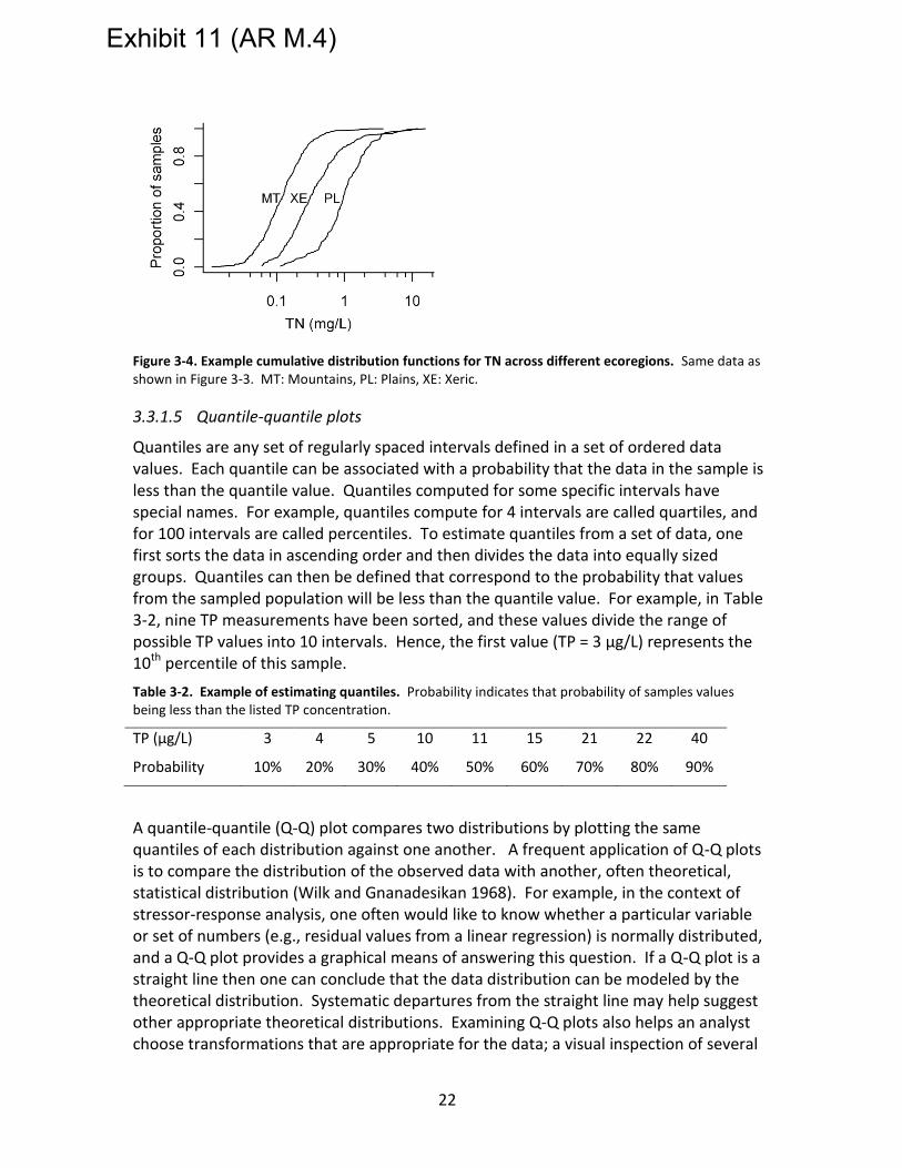
22
Figure 3-4. Example cumulative distribution functions for TN across different ecoregions. Same data as shown in Figure 3-3. MT: Mountains, PL: Plains, XE: Xeric.
3.3.1.5 Quantile-quantile plots
Quantiles are any set of regularly spaced intervals defined in a set of ordered data values. Each quantile can be associated with a probability that the data in the sample is less than the quantile value. Quantiles computed for some specific intervals have special names. For example, quantiles compute for 4 intervals are called quartiles, and for 100 intervals are called percentiles. To estimate quantiles from a set of data, one first sorts the data in ascending order and then divides the data into equally sized groups. Quantiles can then be defined that correspond to the probability that values from the sampled population will be less than the quantile value. For example, in Table 3-2, nine TP measurements have been sorted, and these values divide the range of possible TP values into 10 intervals. Hence, the first value (TP = 3 µg/L) represents the 10th percentile of this sample.
Table 3-2. Example of estimating quantiles. Probability indicates that probability of samples values being less than the listed TP concentration.
TP (µg/L) 3 4 5 10 11 15 21 22 40
Probability 10% 20% 30% 40% 50% 60% 70% 80% 90%
A quantile-quantile (Q-Q) plot compares two distributions by plotting the same quantiles of each distribution against one another. A frequent application of Q-Q plots is to compare the distribution of the observed data with another, often theoretical, statistical distribution (Wilk and Gnanadesikan 1968). For example, in the context of stressor-response analysis, one often would like to know whether a particular variable or set of numbers (e.g., residual values from a linear regression) is normally distributed, and a Q-Q plot provides a graphical means of answering this question. If a Q-Q plot is a straight line then one can conclude that the data distribution can be modeled by the theoretical distribution. Systematic departures from the straight line may help suggest other appropriate theoretical distributions. Examining Q-Q plots also helps an analyst choose transformations that are appropriate for the data; a visual inspection of several
Exhibit 11 (AR M.4)

23
candidate transformations can provide an indication of which transformation better conforms to a desired theoretical distribution. For example, Q-Q plots for TN values in EMAP-West indicate that log-transformed values are more normally distributed than measurements in their original units (Figure 3-5).
Figure 3-5. Quantile-quantile plots comparing TN (left plot) and log(TN) (right plot) values from EMAP-West to normal distributions. Solid line is drawn through the 1
st and 3
rd quartiles (shown as filled black
circles) to help visualize the degree to which samples fall on a straight line. Units are µg/L (left plot) and log-transformed µg/L (right plot).
3.3.2 Bivariate summary and visualization methods
Relationships between pairs of variables are the fundamental relationships that underlie stressor-response analyses. In addition to considering the structure of the conceptual model, a clear understanding of which pairs of variables are related also helps identify variables that may confound subsequent estimates of nutrient stressor-response relationships.
3.3.2.1 Correlation analysis
Correlation analysis is a method for measuring the degree to which the values of two variables change together across different samples. The correlation coefficient quantifies the strength of the relationship between two variables and is a unitless number that varies from -1 to +1. The magnitude of the correlation coefficient is the standardized degree of association between the two variables. The sign is the direction of the association, which can be positive or negative. A coefficient near 0 indicates that the two variables are not related. A negative coefficient indicates that as the value of one variable increases, the other decreases. A positive coefficient indicates that as the value of one variable increases the other also increases. Larger absolute values of coefficients indicate stronger associations; however, in some cases small coefficients may be due to a nonlinear relationship.
Two types of correlations are used most frequently. Pearson's product-moment correlation coefficient, r, measures the degree of linear association between two
Exhibit 11 (AR M.4)

24
variables. Spearman's rank-order correlation coefficient (ρ) uses the ranks of the data, relaxing the linearity assumption of r, and can provide a more robust estimate of the degree to which two variables are monotonically associated even if the relationship is non-linear.
Examining scatter plots (Section 3.3.2.2) supplements the insights provided by correlation coefficients.
3.3.2.2 Scatter plots
Scatter plots are used to visualize the relationship between two variables. In addition to indicating how strongly two variables are related, scatter plots can indicate whether a straight line or other functional form can reasonably represent an observed relationship.
An example scatter plot of TN versus a multimetric macroinvertebrate index of biological condition (MMI) is shown in Figure 3-6. Decreases in MMI are associated with increases in TN concentration, but the variability in sample values about the mean relationship is large.
A scatter plot matrix provides a means of simultaneously viewing all pairwise relationships within a set of several variables. Two variables, labeled along the main diagonal of the figure, are plotted against each other in each panel of the matrix. For example, in the panel in the lower left hand corner of Figure 3-7, log TN is plotted on the horizontal axis versus percent sand/fines on the vertical axis. This visualization of relationships among variables can assist in identifying variables from conceptual models that may confound estimates of stressor-response relationships. In this example, log TN and log TP covary strongly with one another, and with percent sand/fines and grazing. As different nutrients originate from similar sources, TN and TP are generally expected to covary. The covariation of substrate sand/fines and grazing with N and P concentrations indicates that these two variables are possible confounders of estimated nutrient stressor-response relationships.
Exhibit 11 (AR M.4)

25
Figure 3-6. Scatter plot of TN versus a multimetric macroinvertebrate index of stream biological condition (MMI) from the EMAP-West Stream Survey in North and South Dakota, Wyoming, and Montana.
Figure 3-7. Scatter plot matrix of EMAP-West Streams Survey TN and TP (as log-transformed variables) against measures of grazing intensity in the watershed, and percent sand/fine substrates. Units are µg/L for TN and TP. Grazing intensity quantified as a unitless index score.
Exhibit 11 (AR M.4)

26
3.3.2.3 Conditional probability
A conditional probability is the probability of an event Y occurring given that some other event X also has occurred. It is denoted as P (Y|X) and is read as the probability of Y given X. A conditional probability can be estimated as the probability of observing an event of interest in a subset of samples drawn from the original statistical population, in which the subset is defined by conditions when X has occurred. Conditional probability analysis describes the probability of environmental or ecological impairment (i.e., not meeting the designated use) given that a nutrient concentration is higher than some specified value (Paul and MacDonald 2005). For example, conditional probability analysis can quantify the probability of a benthic community impact given that TP concentrations in the water column exceed 0.1 mg/L. To use this visualization approach, a threshold in the response variable is required (e.g., it is assumed here that chl a exceeding 15 µg/L is associated with undesirable conditions).
In EDA, conditional probability analysis can screen variables for use in the development of stressor-response relationships. For example, Figure 3-8 shows conditional probability analysis plots for the EMAP Northeast Lakes Survey data with chl a as the response (using a threshold of 15 µg/L) and with TP and TN as potential predictors because each can potentially affect chl a. Each point on a plot displays the estimated probability of lakes exceeding the chl a threshold given that the indicated stressor level is exceeded. For example, chl a exceeded 15 µg/L in every lake with TP > 0.06 mg/L. This concentration, at which the estimated probability of exceeding the threshold is 100%, could provide an upper bound for candidate N and P criteria.
Figure 3-8. Example plots for conditional probability analysis for EMAP Northeast Lakes Survey data for chl a as response variable (threshold at 15 µg/L) and potential stressor variables TP and TN.
3.3.3 Multivariate visualization methods
Principle component analysis (PCA) is one of the most widely used methods for understanding relationships among many different values (Jolliffe 2002). The method can often represent several inter-correlated variables as a smaller set of principle components that account for the majority of the variability in the data. Each principle component is computed as a weighted sum of the original variables. The weights applied to each variable are known as “loadings”. By reducing the complexity of
Exhibit 11 (AR M.4)

27
multiple variables to a few components, an analyst can more easily visualize similarities and differences among sites and identify groups of variables that covary.
The method is best illustrated using just two variables. In Figure 3-9, principle components are shown for a dataset composed only of log TN and log TP. The first principle component (PC1) identifies the axis along which the majority of the variation in the two variables occurs. The second principle component (PC2) is uncorrelated with the first. The first axis accounts for over 86% of the variation in log TN and log TP values in the dataset, and positions along this axis might be used as an indicator of overall nutrient enrichment.
Figure 3-9. Illustrative example of principle components analysis for two variables. Arrows labeled as PC1 and PC2 show the first and second principle components, respectively.
PCA is usually applied to many more than 2 variables, but the algorithm for identifying principle components is the same: the first principle component identifies the axis along which the most variability in the data can be explained. Then, subsequent axes are identified that are uncorrelated with all previous components, accounting for as much of the remaining variability as possible. Ideally, a few principle components represent the majority of the variability in the set of original variables. Perhaps more importantly, the loadings that specify the degree to which different variables contribute to each principle component can be interpreted in terms of how different variables covary within the dataset.
When PCA is applied to an expanded set of variables from EMAP-West, including log TN, log TP, stream temperature, substrate sand/fines, log chloride ion concentration (Cl-), elevation and log catchment area, the first principle component is loaded on log TN, log TP, and log Cl-, and to a lesser degree on temperature, substrate composition, and catchment area (Table 3-3). The next two principle components identify variability in the dataset that is primarily associated with the elevation of the sampled site (PC2) and the catchment area of the site (PC3). These three components account for 78% of the
Exhibit 11 (AR M.4)

28
total variability in the original set of variables. The results indicate that several in-stream factors covary with N and P concentrations, whereas site elevation and area may covary less with N and P concentration.
Table 3-3. Loadings for first three principle components of EPA-West data.
PC1 PC2 PC3
log TN 0.44 -0.28 0.17
log TP 0.40 -0.28 0.38
Temperature 0.37 0.21 -0.41
Percent substrate sand/fines 0.39 -0.32 0.17
log Cl- 0.42 0.16 0.03
Elevation -0.23 -0.82 -0.41
log catchment area 0.37 0.07 -0.67
Coplots are another useful approach for exploring the effects of multiple variables on a particular response. Coplots classify the data set into different ranges of values for one or more covariates, and then display the relationship between the primary stressor variable of interest (e.g., N and P concentration) and the response within each of the classes. Hence, the effects of the covariates on the estimated relationship can be more easily discerned. The relationship between TN and MMI shown in Figure 3-6 exhibits different trends depending on the levels of bedded fine sediment in the streams (Figure 3-10). At low levels of sediment, MMI appears to decrease with increased TN (lower left panel), but at moderate levels of sediment this relationship weakens (lower middle and right panels). Then, at high levels of sediment, a relatively strong relationship between MMI and TN is observed.
Many other multivariate visualization techniques are available for exploratory data analysis, but are beyond the scope of this document. Interested readers should consult other resources (e.g., Venables and Ripley, 2002) for information regarding these other techniques.
Exhibit 11 (AR M.4)

29
Figure 3-10. Example coplot showing the relationship between TN and MMI for different levels of bedded sediment. Dark orange bar at the top of each panel indicates the range of bedded sediment values included in that panel. Panels are numbered sequentially from low to high levels of bedded sediment. Bedded sediment quantified as percent sand/fines in the substrate.
3.3.4 Mapping data
Mapping data can provide insights into whether factors vary systematically across a geographic area or region. The simplest method is to create a map indicating the locations where the data were collected. More sophisticated maps couple the sample locations with a variable value. Although geographic information systems (GIS) are most frequently used to generate maps, exploratory spatial analysis can be done with most graphics and spreadsheet software applications by simply plotting latitude and longitude values in a scatter plot. This visual presentation is particularly useful for presenting similarities and differences across ecoregions or other spatial classifications.
A map of the locations of sites that were sampled for the EMAP-West Stream Survey, with symbols sized according to TN concentration, shows a spatial trend of increased TN concentration in the eastern part of the mapped region (Figure 3-11). This spatial pattern can be incorporated in subsequent statistical analyses.
Exhibit 11 (AR M.4)

30
Figure 3-11. Map of TN data from EMAP-West Stream survey in North and South Dakota, Montana, and Wyoming. Symbol size is proportional to log TN concentration.
3.3.5 Data issues
3.3.5.1 Data representativeness
The degree to which available data represent the study area should be evaluated during data exploration. Representativeness can influence where and when inferences from a stressor-response relationship would be expected to be valid. For example, if a stressor-response relationship were estimated using data collected in the winter, then use of this relationship to derive criteria applicable in the summer should be considered carefully. Similarly, relationships estimated using data from deep lakes may not be applicable for deriving criteria for shallow lakes.
Mapping available data (Section 3.3.4) can provide insights into the degree to which the data represent the geographical area, while considering the sampling design used to collect the data (Section 3.2.2) can inform decisions regarding temporal representativeness. The degree to which available data represents other potential natural gradients (e.g., lake size, geology, elevation) can be evaluated using the numerical summaries, histograms, and other univariate visualization methods. Ultimately, one should compare the range of conditions in the available data with the range of conditions in which the criteria will apply to determine whether data are sufficiently representative.
3.3.5.2 Missing data
During the initial exploration of assembled data, analysts should consider the extent to which data are missing. Estimates of stressor-response relationships often rely on data collected at the same time and location; and thus, patterns in data that are missing must be considered prior to analysis. Data missing randomly generally have minimal effects on estimated stressor-response relationships, but data missing in a predictable pattern can bias estimated relationships and should be considered further. For example, data can often be missing due to systematic issues encountered during data
Exhibit 11 (AR M.4)

31
collection, such as instrument detection limits. Then, values of the measured variable below this detection limit are unresolved, and stressor-response relationships cannot be estimated for these low values.
A particular variable can be tested statistically for whether it is missing at random by splitting the dataset into one subset in which the variable has a value and one subset in which a value for the variable is missing. Then, other measured variables can be examined for significant differences across the two subsets. If data are missing at random, then samples with missing data can simply be excluded from the data set. If data are not missing at random, then analysts should consider the effect of the missing data. For example, in some cases, a lower detection limit does not influence the analysis because biological effects are not expected at those values of the variable below the detection limit. Alternatively, imputation methods (i.e., use of predicted values to complete the dataset) may be appropriate (Rubin and Little 2002). When a dataset includes a large amount of missing values, it may be necessary to consult a statistician regarding the most appropriate method to either develop a complete dataset or to apply appropriate modeling approaches that can use incomplete data.
3.3.5.3 Outliers
Outliers are data that are far outside of the central distribution. Outliers can strongly affect mean values and estimated stressor-response relationships, so analysts should evaluate outliers during data exploration. Outliers are often identified by visually inspecting the data in histograms and/or scatter plots. In general, outliers should not be excluded from the data set except in cases in which they can be shown to be a result of measurement errors, laboratory errors, or recording errors.
Exhibit 11 (AR M.4)

32
4 Analyze data
This section presents a three-step approach for using stressor-response relationships to derive numeric nutrient criteria, in which data are classified, stressor-response relationships are estimated from the data, and criteria are derived from the relationships.
When using stressor-response relationships to derive criteria, the estimated relationships should represent the relationships shown on the conceptual model as accurately as possible. However, in most cases other environmental variables may influence, or confound, bivariate relationships estimated between a nutrient and a response variable. Hence, in the first step of the analysis, classification, the analyst attempts to control for the possible effects of other environmental variables by identifying classes of waterbodies that have similar characteristics and are expected to have similar stressor-response relationships. Classifications for a stressor-response analysis are typically based on statistical analysis; however, existing classes can be used as a starting point. The most widely used existing classifications for analyses of nutrient data are the fourteen national nutrient ecoregions (Omernik et al. 2000, USEPA 2000a). These ecoregions were designated based on similar climate, topography, regional geology and soils, biogeography, and broad land use patterns. In addition to ecoregions, other qualitative groupings may be readily available (e.g., deep versus shallow lakes). Existing and qualitative classes provide a coarse starting point that should be refined as the analysis proceeds.
Statistical approaches to classification refine initial classes and improve estimates of stressor-response relationships. Because these approaches build upon some of the same regression methods used to estimate stressor-response relationships, they are considered in detail in Section 4.3, after the discussion of methods for estimating stressor-response relationships.
The second step, simple linear regression (SLR), estimates stressor-response relationships within each class. Simple linear regression provides estimates of nutrient stressor-response relationships that can be most easily interpreted for deriving criteria. In the third step, criteria are derived based on a probabilistic interpretation of the estimated stressor-response relationships. In some special cases, extensions of simple linear regression (e.g., multiple linear regression) may be necessary, but interpretation of the results of these more complex analyses are facilitated by a thorough understanding of simple linear regression.
In general, substantial iteration between classification, estimating stressor-response relationships, and deriving criteria is expected.
4.1 Simple linear regression
Simple linear regression (SLR) provides an estimate of the linear relationship between a response variable and an explanatory variable (e.g., a stressor such as the concentration
Exhibit 11 (AR M.4)

33
of N or P). The results of SLR are two coefficients specifying the intercept and slope of a straight line representing the modeled relationship between the two variables.
SLR requires a certain amount of data to provide reliable results. Harrell et al. (1996) suggests the use of a minimum of ten independent samples per degree of freedom in the model. Hence, the two coefficients estimated in SLR require the use of at least 20 independent samples when fitting the model.
SLR can estimate a relationship between any pair of variables. However, when used for criteria derivation, relationships estimated with SLR predict likely values of the dependent variable at a new value of the independent variable. For example, a regression relationship may predict the future concentration of chlorophyll-a (chl a) at a new N or P concentration. When used in this way, it is important to consider the theoretical assumptions underlying SLR inferences. More specifically, one must assess: (1) whether the assumed linear functional form is sufficiently representative of the actual relationship, (2) whether the sampling variability in the dependent variable is distributed as assumed, (3) whether the magnitude of the sampling variability in the dependent variable changes across the range of predictions, and (4) whether the samples used to fit the model are independent of one another.
Each of these assumptions is discussed in more detail, but first, a simple example is introduced to illustrate analytical techniques discussed in this section.
4.1.1 Example data set
As discussed earlier, monitoring data most frequently available for estimating stressor-response relationships consist of one or two measurements of different variables collected from locations distributed across a state or ecoregion (i.e., synoptic monitoring data). However, to better illustrate the use of SLR to estimate stressor-response relationships, it is useful to first consider the simplified case of data collected regularly from a single location over a long period of time. This initial example is expanded incrementally to address the use of synoptic monitoring data for stressor-response analysis.
In this example, the data used are TN and chl a measurements collected regularly from a single lake during spring and summer (March – August) over 10 years. A strong relationship exists between TN and chl a in this lake (Figure 4-1). Because these data were collected from a single lake, many environmental factors (e.g., lake depth) are assumed constant. The influence of some of the other factors that may covary with N or P concentrations within the same lake, such as temperature and light availability, can be partially controlled by considering only data collected at approximately the same time of the year, such as the same season. By definition, the remaining variability in observed values of chl a about the mean relationship with TN (appearing as the scatter of points about the solid line) can be attributed to variations in conditions within this particular lake. For example, slight differences among samples with respect to the time of day a sample was collected or the location on the lake at which the sample was collected can
Exhibit 11 (AR M.4)

34
affect the measured chl a concentration. Approaches for interpreting this within-lake variability when deriving criteria are discussed in Section 4.1.3.
Figure 4-1. Total nitrogen (TN) versus chlorophyll a (chl a) in one lake collected during March-August over 10 years. Solid line: simple linear regression fit.
4.1.2 Simple linear regression assumptions
4.1.2.1 Linear functional form
The first regression assumption to evaluate is whether a straight line provides an appropriate representation of the relationship that is modeled. A statistical approach for evaluating this assumption is to compare the degree to which a straight line accounts for observed variability in the dependent variable with a nonparametric regression curve that relaxes this requirement (see Section 4.2.3). Ecological knowledge or visual inspection of the data (e.g., Figure 4-1) often can provide sufficient insight into whether a linear approximation is appropriate.
4.1.2.2 Distribution of errors
To use regression to accurately predicting future conditions, the distribution of the error in observed values of the dependent variable about the estimated mean relationship must be similar to the assumed theoretical error distribution. In SLR, it is assumed that the errors in the dependent variable are normally distributed. That is, for each value of the independent variable, the distribution of the distances of the observed values from the mean relationship is assumed to follow a normal (Gaussian) distribution.
One way to assess whether this assumption holds true for a particular data set is to compare the distribution of residual values with a normal distribution. A residual value is defined as the difference between the modeled mean value and the observed value for a particular sample. In Figure 4-1, the residual value for each sample is the vertical distance between the sample and the mean regression line. Overall, the distribution of
Exhibit 11 (AR M.4)

35
residual values should be nearly normal for SLR. Quantile-quantile plots provide a robust, graphical approach for assessing whether residuals are normally distributed (see Section 3.3.1.5). In the example shown in Figure 4-2, most values cluster around the solid line, indicating a near-normal distribution. However, departures of samples at the upper and lower end from a straight line suggest that residuals extend to slightly more extreme values than predicted by a normal distribution. More severe departures from normality indicate that data cannot be modeled effectively with this assumption.
Figure 4-2. Quantile-quantile plot comparing residuals from the relationship shown in Figure 4-1 with a normal distribution. Solid line is drawn through the 1
st and 3
rd quartiles to help visualize the data.
In assessing the assumption of normal sampling variability, it is often useful to consider the known characteristics of the response, or dependent variable. Many typical response variables are not normally distributed. For example, variables that measure a count (e.g., total taxon richness) have a minimum value of 0, and those that measure a proportion (e.g., relative abundance) have a minimum value of 0 and a maximum value of 1. Normal distributions do not allow for such constraints, and therefore, may not be appropriate. However, some variables may appear to be constrained but are reasonably well approximated by a normal distribution (e.g., multimetric biological indices, total richness values that are much greater than zero). Other variables that have a minimum value of zero and are strongly skewed to the right (e.g., chemical concentrations, watershed area) can be normally distributed after a log transformation (see Section 3.3.1). Similarly, variables that quantify a proportion (e.g., relative abundance) often can be used in SLR after transforming with an arcsine-square root. Generalized linear models (McCullagh and Nelder 1991) allow one to directly model certain types of data with non-normal distributions, but use of these models is more complex and may require that one consult a professional statistician.
Exhibit 11 (AR M.4)

36
4.1.2.3 Magnitude of errors
Predicting future conditions using a regression relationship also assumes that the magnitude of the variance of errors about the mean line is constant for all predicted values. A straightforward method for testing this assumption is to plot residual values against predicted values and assess whether the scatter of the residual values is constant over the entire range of fitted values. For the relationship shown in Figure 4-1, this assumption seems reasonably well supported, although the magnitude of residual variability does seem slightly larger for low predicted chl a values (Figure 4-3). Other common phenomenon include residual variance that increases with increases in fitted values (e.g., trumpet-shaped plots), which would suggest that sampling variance is not constant, and certain inferences from the regression relationship may not be accurate.
When the magnitude of residual variability varies strongly across predicted values, quantile regression provides an alternate approach for estimating characteristics of the relationships for criteria derivation (see section 4.2.2).
Figure 4-3. Residuals from regression fit shown in Figure 4-1 plotted versus predicted values.
4.1.2.4 Sample independence
Regression models typically assume that samples are independent from one another, and when this assumption is violated, more confidence may be ascribed to results than is supported by the data. Statistical approaches for evaluating sample independence are beyond the scope of this guidance, but analysts should qualitatively consider whether samples in a dataset are potentially related. For example, samples collected from closely spaced locations along the same river might be related to one another, and should not be included in the same regression analysis.
4.1.2.5 Other diagnostic statistics
Several other diagnostic statistics are frequently reported with SLR results by statistical software, including standard errors on coefficient estimates, statistical significance of each model coefficient, and R2 values. Standard errors quantify the uncertainty in the estimates of each coefficient value, while statistical significance tests, such as the t-test,
Exhibit 11 (AR M.4)

37
provide an interpretation of these standard errors with respect to a null hypothesis. More specifically, the significance tests provide an estimate of the probability that the observed data would have occurred if some pre-specified null hypothesis were true. For example, the null hypothesis for the coefficient measuring the slope of the line is that the value of this coefficient is zero. Therefore, the “p-value” provided in typical regression output provides an estimate of the probability that the observed data would have occurred if the slope of the relationship were zero. The statistical significance of the slope of the estimated relationship between the nutrient variable and the response variable provides some indication of whether the relationship exists beyond what one would expect from chance alone.
The coefficient of determination (R2) measures the proportion of variance in the response that is explained by the regression model. R2 values near 1 indicate that the selected independent variable accounts for a large proportion of the observed variability in the dependent variable. R2 values must be interpreted in the context of a priori expectations for model performance. For example, the value of some response variables may change substantially in successive samples from the same location simply due to sampling variability. For these variables, one would expect the regression model to account for a smaller proportion of the observed variability compared with a situation in which the sampling variability of the response variable exhibits very low variability. No single R2 value can be pre-specified that indicates the differences between acceptable and unacceptable stressor-response models, and R2 is more effectively used to compare among different candidate models for the same response variable.
4.1.3 Deriving candidate criteria from stressor-response relationships
A stressor-response relationship estimated by SLR predicts the value of the response variable, given a particular nutrient concentration. Hence, if the value of the response variable that supports the designated uses is known for a waterbody, the stressor-response relationship can “translate” this response threshold to a numeric criterion value. In many cases, a threshold for the selected response variable is available that defines values of the response variable where designated uses are supported. For chemical acute water quality criteria, the US EPA has defined this threshold as the lower 5th percentile of the distribution of applicable acute values, a value that represents a low overall effect level to species in the broader ecosystem (US EPA 1985). A comparable approach is not applicable to deriving water quality criteria for nutrients because adverse effects to the designated use of a waterbody occur at concentrations of N and P below the level that is shown to be toxic to organisms (see, for example, toxic concentrations for nitrate in US EPA 1986). Alternative approaches for establishing thresholds for response variables are available, though. For example, a protective level may be pre-determined if criteria already exist in state standards to protect the designated use (e.g., biological criteria). Also, expert opinion regarding appropriate protective levels of variables can be formally elicited (Reckhow et al. 2005), and surveys can be conducted to identify conditions that conform with user expectations for
Exhibit 11 (AR M.4)

38
different waterbodies (Heiskary and Walker 1988). For the examples shown in this document, it is assumed for illustrative purposes that lake chl a concentrations exceeding 20 µg/L indicate impaired aquatic life use.
4.1.3.1 Prediction and confidence intervals
Prediction intervals provide useful information when deriving criteria from stressor-response relationships because they depict the uncertainty in predicting a single response value (e.g., chl a concentration) at a given value of the explanatory variable (TN concentration in this case). So, on average, 90% of future chl a values sampled at a particular value of TN would be located within the range defined by the 90% prediction intervals1. Similarly, on average, 95% of chl a values would be less than the value specified by the upper prediction interval for a particular value of TN. Criterion values can be based on the intersection of different prediction intervals with the selected biological threshold. For this lake, the upper 90% prediction interval intersects chl a = 20 μg/L at TN = 0.66 mg/L, the lower prediction interval intersects at TN = 1.56 mg/L, and the mean relationship intersects at TN = 1.02 mg/L (Arrows A, C, and B, respectively in Figure 4-4).
Selecting a particular criterion from this range of values depends in part on the tolerance for excursions above the threshold value for chl a. For example, the model predicts that on average 95% of future chl a measurements at TN = 0.66 mg/L will be less than 20 μg/L, and so an analyst might select 0.66 as a criterion value to assure that chl a rarely, if ever, exceeded the stated threshold in any single sample that met the TN criterion (i.e., TN ≤ 0.66 mg/L). Alternatively, an analyst might select 1.02 mg/L to maintain an average chl a concentration over all samples in the lake of 20 μg/L. That is, if TN concentrations were maintained at or below 1.02 mg/L, then average chl a concentrations should be less than or equal to 20 μg/L.
Criteria based on other prediction intervals can be interpreted in a similar manner. For example, a criterion based on the point at which the 75th percentile of the predicted distribution was equal to 20 μg/L would be interpreted as the TN concentration at which 75% of future chl a measurement would be less than or equal to 20 μg/L.
Selection of the appropriate criterion value within the range defined by the prediction intervals is ultimately a management decision; however, this decision can be informed by an assessment of the sources of the prediction uncertainty. For example, if the majority of within-lake variability can be attributed to measurement error (e.g., variations due to random errors in a measurement method), one could select the
1 Tolerance intervals specify a range of response values in which we expect a certain proportion of future
observations to fall, with some pre-specified probability. For example, with tolerance intervals, one can compute a range of values that will contain 90% of subsequent chl a values with a probability of 95%. Prediction intervals as described here are equivalent to specifying a tolerance interval with a 50% probability. That is, there is a 50% probability that 90% of future chl a value will fall within the 90% prediction intervals. See Proschan (1953) and Vardeman (1992) for more details.
Exhibit 11 (AR M.4)

39
criterion associated with the mean stressor-response relationship. Conversely, if within-lake variability was primarily associated with systematic, temporal changes in lake characteristics (e.g., changes in degree of stratification), then one defensible approach could be to select the criterion associated with the upper prediction interval, to maintain the desired chl a concentration in spite of the uncertainties in the stressor-response model.
Figure 4-4. Total nitrogen (TN) versus chl a in one lake collected during March-August over 10 years. Solid line: linear regression fit. Dashed lines: upper and lower 90th prediction intervals. Red horizontal line: chl a = 20 µg/L. Note that upper prediction interval has been extended beyond the range of the data to estimate the point at which it intersects the chl a threshold. Arrows indicate candidate criteria associated with different prediction intervals and the mean relationship. See text for details.
Note that the upper prediction interval in Figure 4-4 must be extended, or extrapolated, beyond the range of the data to identify an intersection point with the chl a threshold (Arrow A in Figure 4-4). Extrapolation introduces an additional source of uncertainty to the estimated criterion values, and the magnitude of this uncertainty increases with the distance between the observed data and the extrapolated point. In this case, the extrapolated criterion value is only 0.1 mg/L less than the minimum observed TN value in the data, and likely introduces a small amount of additional uncertainty. In addition to considering the distance one is extrapolating beyond observed data, other questions one might consider when evaluating the defensibility of extrapolation include the following: is the period of record particularly short for this lake, therefore limiting the range of sampled conditions, and would we expect this lake to behave differently at nutrient concentrations below those that are available in the data set?
Confidence intervals can also provide useful information when deriving criteria from stressor-response relationships. Confidence intervals depict the uncertainty inherent in estimating a mean response value, given the value of the explanatory variable (Figure 4-5). Hence, confidence intervals are narrower than prediction intervals. For example, if TN = 1.02 mg/L, the relationship indicates that the mean chl a concentration across
Exhibit 11 (AR M.4)

40
many samples is 20 µg/L. The number of samples used in this example is relatively large, and so, the mean value can be estimated with a high degree of confidence. Compared with using the mean chl a and prediction intervals to derive a range of possible criteria (see Figure 4-4), criterion values associated with maintaining mean chl a = 20 µg/L span a narrower range (0.96 to 1.08 mg/L TN around the mean criterion of 1.02 mg/L).
Figure 4-5. Total nitrogen (TN) versus chl a in one lake collected during March-August over 10 years. Solid line: linear regression fit. Dashed lines: upper and lower 90
th confidence intervals.
4.1.3.2 Averaging data
In some cases, averaging single samples over pre-defined time intervals may provide stressor-response relationships that more closely match the timescale for which criteria are desired. For example, if a criterion based on annual or seasonally averaged concentrations is desired, then stressor-response relationships should be estimated using similarly averaged data. Seasonally or annually averaged data can also more closely represent the concepts shown in the conceptual model. For example, seasonally averaged nutrient concentrations may be a more accurate quantification of the overall loading of nutrients into a particular waterbody (Dillon and Rigler 1974).
In general, averaging multiple measurements reduces the variability of both the stressor and response variables (e.g., TN and chl a), and thus, changes the estimated stressor-response relationship. The data shown in Figure 4-4 was averaged by year, giving annual average spring/summer chl a and TN concentrations (Figure 4-6). The mean line estimated for the annual averaged data in this case gives a criterion of 1.08 mg/L TN (arrow B in Figure 4-6) while the upper 90% prediction interval gives a criterion value of 0.79 mg/L (arrow A in Figure 4-6). Note again that the upper prediction interval must be extended beyond the limits of the data to estimate its intersection point with the biological threshold value.
Exhibit 11 (AR M.4)

41
Averaging data reduces the sample size, and hence, increases the width of the confidence intervals about the mean stressor-response relationship. Criterion values ranging from 0.92 to 1.17 mg/L TN are associated with maintaining seasonally averaged chl a at 20 µg/L (Figure 4-7).
Figure 4-6. Seasonally averaged TN versus chl a from March-August. Same data as shown in Figure 4-4. Solid line: linear regression fit. Dashed lines: upper and lower 90th prediction intervals. Red horizontal line: chl a = 20 µg/L. Arrows indicate candidate criterion values associated with different prediction intervals and the mean relationship (see text for details). Note that upper prediction interval has been extended beyond the range of the data to estimate the point at which it intersects the chl a threshold.
Figure 4-7. Seasonally averaged TN versus chl a. Solid line: linear regression fit. Dashed lines: upper and lower 90th confidence intervals.
Exhibit 11 (AR M.4)

42
4.1.3.3 Group of similar lakes
In most cases, a single criterion value is needed that applies to all waterbodies within a region. One way to better understand the uncertainties inherent in this approach is to consider data collected over time from several lakes that are assumed to be similar in terms of other environmental factors, such as color or depth. Within the lakes selected for this example, the annual-averaged chl a concentrations respond similarly to increases in annual-averaged TN (i.e., the slopes of the stressor-response relationships are nearly identical) (Figure 4-8).
Figure 4-8. Annual average TN versus chl a in several similar lakes. Different symbols indicate different lakes. Lines indicate linear regression fits for TN-chl a relationship within each lake. Arrows indicate range of criteria associated with different lakes.
Figure 4-9. Estimated slopes for TN versus chl a relationships in each of the five lakes shown in Figure 4-8. Vertical bars show 90% confidence intervals on estimated slopes.
Exhibit 11 (AR M.4)

43
90% confidence intervals on estimates of the slope of each line can be estimated by adding and subtracting 1.64 times the standard error on each slope.2 A plot of these confidence intervals provides further confirmation that the slopes are statistically indistinguishable from one another (Figure 4-9). Note that for this example, lakes were selected such that their stressor-response relationships were similar. In general, classifying different waterbodies with respect to appropriate environmental variables will increase the likelihood that stressor-response relationships are similar (see Section 4.3).
Even though the slopes of the stressor-response relationships are similar across different lakes, slight differences in the natural conditions (e.g., lake depth) give rise to differences in the position of the stressor-response relationship (i.e., the intercept of the stressor-response relationship). Thus, one might assign slightly different criteria for each lake, ranging from 0.98 to 1.57 mg/L, corresponding to the points at which each mean stressor-response relationship intersects the threshold value for chl a (arrows labeled A and B in Figure 4-8). Criteria for each lake can also be derived from the intersection of upper prediction intervals and the threshold chl a value, yielding values that range from 0.63 to 1.08 mg/L TN (Figure 4-10). Instead of assigning different criterion values to each lake, a more common approach would be to set one criterion value that would apply to this group of lakes. For example, selecting the minimum criterion value estimated across all lakes in Figure 4-8 would ensure that average chl a concentrations were maintained at 20 μg/L or lower for all lakes. However, this single criterion value is lower than is required to maintain chl a = 20 μg/L for certain lakes in the group.
In some lakes the range of available data may not include the chosen biological threshold, or the estimated stressor-response relationships may not intersect the biological threshold. Similar to previous examples, one must consider whether extrapolating beyond the available data is defensible.
2 Confidence limits on estimates of a mean value from a finite set of samples are derived from normal
probability theory. The interval bounded by (–1.64 × standard error, 1.64 × standard error) corresponds to a range of values in which there is a 90% chance that the true population mean value will be located.
Exhibit 11 (AR M.4)

44
Figure 4-10. Upper prediction intervals for TN-chl a relationships in several similar lakes. Dashed lines show the upper 90% prediction intervals. Different symbols indicate different lakes.
4.1.3.4 Synoptic monitoring data
As discussed earlier, data most frequently available for estimating stressor-response relationships are collected using synoptic sampling designs, in which one or two measurements are collected during the same time period from many different locations across the study area. For example, only two seasonally averaged values of TN and chl a might be collected from each of the lakes shown in Figure 4-8 under a synoptic sampling design (Figure 4-11). In this case, the slope of the stressor-response relationship estimated from the synoptic data is similar to that estimated for individual lakes (see Figure 4-8), and the criterion value associated with the mean relationship is 1.1 mg/L TN, which is within the range of values estimated for individual lakes.
Prediction intervals for this relationship now reflect both within-lake and across-lake variability, and interpretation of these prediction intervals with respect to setting a criterion should account for these two sources of variability. Several options for using these prediction intervals to set criteria are possible. First, one can set the criterion value at the point where the upper prediction interval intersects the biological threshold. Setting the TN criterion at this point assures that annual chl a concentration in any single lake rarely exceeds the threshold of 20 µg/L and that we are selecting the minimum TN criterion estimated from all lakes in the group. That is, this first option corresponds with selecting the minimum criterion value estimated from the upper prediction intervals of each individual lake (see Figure 4-10) 3.
3 This comparison holds true statistically when relatively large numbers of samples are available for each
individual lake. When sample sizes are small within individual lakes, prediction intervals for each lake model will also reflect the uncertainty in estimating a relationship from a small amount of data, and therefore prediction intervals may be broader than those estimated across a large synoptic data set.
Exhibit 11 (AR M.4)

45
Figure 4-11. Synopic data set simulated by selecting 2 annual average values from each lake (shown as filled black circles). Open gray circles show all of the available seasonally averaged data to facilitate comparison with previous examples. Solid line shows linear regression fit to the synoptic data (filled black circles) and dashed lines show 90% prediction intervals.
A second option is to explicitly estimate the magnitude of both within- and across-lake variability and to use these estimates to derive candidate criteria. That is, with sufficient data from within individual lakes and across different lakes, one can estimate contributions of each of these sources of variability to the observed relationships. Then, criteria can be specified that account for management decisions regarding both of these types of variability. For example, one might specify a criterion that allowed chl a concentrations to exceed a threshold in 20% of the samples from any single lake, but only exceeded the threshold in 5% of the lakes in the region. Hierarchical Bayesian models (Gelman et al. 2009) and linear mixed effects models (Pinheiro and Bates 2000) are two statistical approaches for estimating the magnitudes of different sources of variability in a single data set, but these methods are beyond the scope of this document. Consultation with a statistician is recommended.
A final option for using prediction intervals from synoptic data to specify criteria is to adjust the selection of the appropriate prediction interval based on a qualitative evaluation of within- and across-lake sources of variability. For example, knowing that the prediction intervals include both sources of variability, one might select a lower percentile of the predicted distribution (e.g., the 75th rather than the 90th percentile) to derive candidate criteria.
Differences between relationships estimated within a particular waterbody and relationships estimated across a set of similar waterbodies are often discussed in terms of a “space-for-time” substitution (Fukami and Wardle 2005). That is, a relationship estimated across different waterbodies in space is substituted for the relationship of interest, which is one estimated for each waterbody in time. The space-for-time substitution was appropriate in the preceding example because the stressor-response
Exhibit 11 (AR M.4)

46
relationship estimated from the composite, sampled data set was similar to relationships estimated from individual lakes. In general, though, defining conditions in which this substitution is valid is an important consideration when estimating stressor-response relationships. A group of waterbodies that are similar in all regards except with regard to their nutrient concentrations is likely to satisfy space-for-time assumptions, and identifying these groups is one of the primary goals of classification (see Section 4.3).
4.1.4 Estimating prediction intervals by projection
An alternate approach for estimating prediction intervals for a stressor-response relationship is to predict the distribution of the values of the response variable in a study area, given a candidate numeric criterion value. This approach is best described by considering an example from a single lake (see Figure 4-6) in which the distribution of chl a concentrations is predicted, given the assumption that a criterion value of TN = 1.1 mg/L is applied. (This criterion value corresponds with the intersection between the mean stressor-response relationship and the threshold chl a concentration of 20 µg/L. See Section 4.1.3). A new distribution of chl a concentrations is calculated by first assuming that any sample with TN concentration exceeding the candidate criterion value is managed such that TN concentration is reduced to the criterion value. Then, in each of these samples, a new chl a value is computed using the estimated stressor-response relationship. Examples of these projections are shown as arrows in Figure 4-12, where the slope of each arrow is identical to the slope estimated from SLR. The arrow extends from the observed values of TN and chl a to the candidate criterion value for TN and a predicted value of chl a. Only samples with TN concentrations that exceed the candidate criterion of TN = 1.1 mg/L are projected.
Figure 4-12. Projecting chl a values to a candidate criterion value. Arrows show the projection of sample values using estimated stressor-response relationship to a criterion value of TN = 1.1 mg/L. Projections are only calculated for samples in which TN concentration exceeds the candidate criterion value.
Exhibit 11 (AR M.4)

47
By computing a different prediction for each distinct sample, the inherent variability of observations about the mean regression line has been retained. Because a portion of this variability is caused by random factors, the model prediction for a single sample should not be interpreted as an accurate projection of conditions for that particular sample at a lower TN concentration. However, the overall distribution of predicted values is likely similar to the distribution of values one would observe at the new TN concentration.
Estimates of the slope of the stressor-response relationship are also uncertain (see Figure 4-7), and this uncertainty can affect the distribution of values one would expect to observe. One approach to account for this uncertainty is to repeat the projection using the values corresponding to the upper and lower ends of the confidence interval of the estimated slope of the regression line. The differences in the predicted distribution then would provide an estimate for the effects of uncertainty in the stressor-response relationship. However, when the number of samples used to estimate the stressor-response relationship is large, the uncertainty in estimates of the mean slope is likely small relative to the residual variability about the regression line, and this uncertainty can be ignored when computing projections.
Predicted response values at a new concentration provide information that is directly analogous to prediction intervals that are inferred from SLR. That is, the distribution of projected values should be nearly identical to the distribution that is inferred for a given concentration based on prediction intervals. For example, in Section 4.1.3, the TN = 1.1 mg/L criterion is interpreted as the value necessary to maintain average chl a concentrations at 20 µg/L, and the current predictions are consistent with this interpretation because projected values of chl a at TN = 1.1 mg/L are evenly distributed about 20 µg/L. The advantage of explicitly predicting the values of the response variable in different samples at a new nutrient concentration is that more complex models (e.g., different stressor-response relationships for different classes) can be incorporated into predicted distributions.
A useful extension of this approach is to predict conditions for different waterbodies in a study area. Consider, for example, synoptic data collected from five different lakes, with possible criteria ranging from 0.8 to 1.5 mg/L TN (see Figure 4-11). Suppose now that one sets a criterion value for TN = 1.1 mg/L, and suppose that lakes at which the candidate criterion was exceeded were managed such that TN was reduced to the criterion value. We again project conditions from TN and chl a values in two samples collected from each lake to a TN concentration equal to the candidate criterion value and a predicted value of chl a (Figure 4-13).
Exhibit 11 (AR M.4)
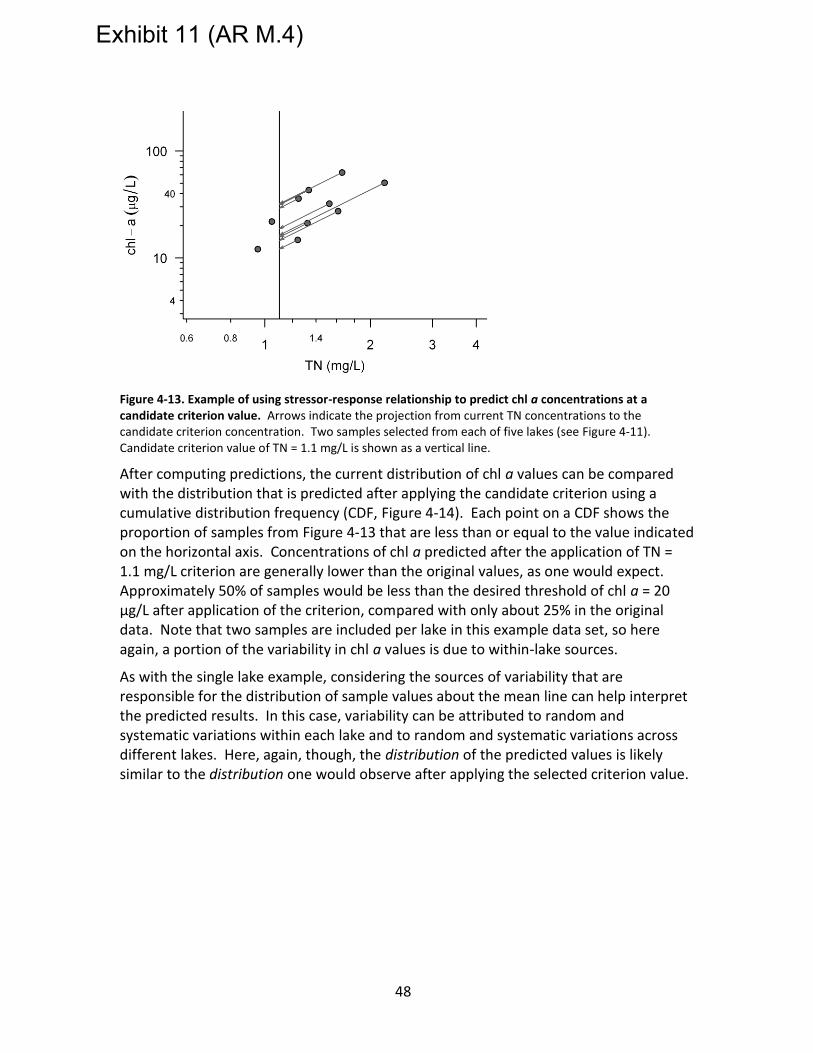
48
Figure 4-13. Example of using stressor-response relationship to predict chl a concentrations at a candidate criterion value. Arrows indicate the projection from current TN concentrations to the candidate criterion concentration. Two samples selected from each of five lakes (see Figure 4-11). Candidate criterion value of TN = 1.1 mg/L is shown as a vertical line.
After computing predictions, the current distribution of chl a values can be compared with the distribution that is predicted after applying the candidate criterion using a cumulative distribution frequency (CDF, Figure 4-14). Each point on a CDF shows the proportion of samples from Figure 4-13 that are less than or equal to the value indicated on the horizontal axis. Concentrations of chl a predicted after the application of TN = 1.1 mg/L criterion are generally lower than the original values, as one would expect. Approximately 50% of samples would be less than the desired threshold of chl a = 20 µg/L after application of the criterion, compared with only about 25% in the original data. Note that two samples are included per lake in this example data set, so here again, a portion of the variability in chl a values is due to within-lake sources.
As with the single lake example, considering the sources of variability that are responsible for the distribution of sample values about the mean line can help interpret the predicted results. In this case, variability can be attributed to random and systematic variations within each lake and to random and systematic variations across different lakes. Here, again, though, the distribution of the predicted values is likely similar to the distribution one would observe after applying the selected criterion value.
Exhibit 11 (AR M.4)

49
Figure 4-14. Cumulative distribution frequencies of chl a values. Original distribution shown as open circles, and predicted distribution for a criterion value of TN = 1.1 mg/L shown as filled circles.
4.2 Extensions of simple linear regression
In certain cases, the assumptions of SLR are too restrictive to accurately model observed data. In this section, different modeling approaches are presented that extend SLR by relaxing one or more of its assumptions. Multiple linear regression is used when the effects of several different factors must be modeled simultaneously, quantile regression is used when residuals are not normally distributed with constant variance, nonparametric regression curves are used when straight lines do not adequately represent the relationship between the stressor and the response, and nonparametric changepoint analysis provides a modeling approach that can represent a sharp change in response values at a particular stressor value.
4.2.1 Multiple linear regression
Multiple linear regression extends SLR to provide an estimate of the linear relationships between one dependent variable and two or more independent variables. In its simplest form, each explanatory variable is assumed to exert an effect on the response that is independent of the effects of the other variables. Multiple linear regression is useful in cases in which other environmental factors in addition to the nutrient variable influence the response, or in cases in which the effects of different nutrients must be modeled together. In general, a classification approach (see Section 4.3) for controlling for other factors coupled with SLR provides more easily interpreted results because the results from SLR can be easily displayed and interpreted graphically. However, in some cases after classifying, modeling different effects simultaneously is still necessary. One such situation is the case in which observed values of the response variable are influenced by both N and P.
Exhibit 11 (AR M.4)

50
Figure 4-15. Modeled relationship between TP, TN, and chl a. Plotted circles indicate combinations of TN and TP values observed in the data, and contour lines indicate modeled mean chl a concentrations (µg/L) associated with particular combinations of TN and TP.
In Figure 4-15, a multiple linear regression example is shown for one lake in which both TN and TP are statistically significant predictors of chl a. That is, chl a concentrations are predicted using the following model,
)log()log()log( 210 TNbTPbbachl
where b0, b1, and b2 are regression coefficients. Thus, both TN and TP criteria must be specified to achieve a desired chl a concentration. For example, to maintain an average chl a concentration of 40 µg/L, one might specify criterion for TN = 1.6 mg/L, which would then dictate a TP criterion of about 0.035 mg/L. A lower TN criterion would require a higher TP criterion to maintain the same average chl a concentration.
Multiple linear regression relies on the same assumptions as SLR, and so, before making predictions with a multiple regression model, analysts should consider whether a linear model form is appropriate, whether the distribution of residual values are normal, and whether the magnitude of residual variances is constant. Additionally, with multiple regression models analysts should evaluate whether different explanatory variables or whether linear combinations of explanatory variables are strongly correlated because including such variables in the model can greatly increase the uncertainty of estimates of regression coefficients. Examining variance inflation factors can provide insights into whether correlated explanatory variables are a problem (see Kutner et al. 2004 for more details).
As more explanatory variables are included, overfitting the model becomes a greater concern. When models are overfitted, they have poor predictive power outside the
Exhibit 11 (AR M.4)

51
calibration data. As discussed earlier, in general, 10 independent samples are usually required per degree of freedom in the model. For example, a model that is described by one intercept value and coefficients for each of three explanatory variables would require at least 40 independent samples (Harrell et al. 1996).
4.2.2 Quantile regression
Quantile regression is an approach for estimating relationships between pairs of variables that relaxes some of the distributional assumptions of SLR. More specifically, quantile regression directly estimates the relationship between a specified quantile (or, percentile) of the response variable with respect to one or more explanatory variables (Koenker and Bassett 1978, Koenker and Hallock 2001, Cade and Noon 2003, Koenker 2005). As with SLR, the relationship is often assumed to be a straight line.
Figure 4-16. Example of quantile regression. Same data as shown in Figure 4-1. Solid black lines are the 5th and 95th percentiles. Red horizontal line shows the response threshold of chl a = 20 µg/L.
Quantile regression provides an alternate approach for estimating prediction intervals that are not subject to the SLR assumptions that residuals are normally distributed and have a constant variance across the range of predictor variables. When applied to the same single lake data shown in Figure 4-1, quantile regression estimates of the 5th and the 95th percentiles include a broader range of chl a values at low TN concentrations (Figure 4-16). These quantiles are very similar to the 90% prediction intervals computed from SLR and can be interpreted in the same way for criterion derivation4. That is, the intersection of the 95th percentile line and the desired response value of chl
4 Regression quantiles only provide an estimate of prediction intervals because they do not include
uncertainty in the estimates of regression parameters (i.e., the slope and intercept of the mean relationship). The magnitude of this uncertainty decreases as the number of samples increases, and so regression quantiles provide better estimates of prediction intervals with larger datasets.
Exhibit 11 (AR M.4)
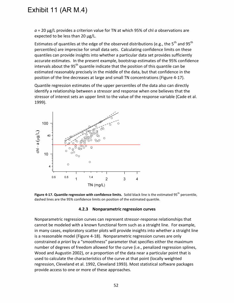
52
a = 20 µg/L provides a criterion value for TN at which 95% of chl a observations are expected to be less than 20 µg/L.
Estimates of quantiles at the edge of the observed distributions (e.g., the 5th and 95th percentiles) are imprecise for small data sets. Calculating confidence limits on these quantiles can provide insights into whether a particular data set provides sufficiently accurate estimates. In the present example, bootstrap estimates of the 95% confidence intervals about the 95th quantile indicate that the position of this quantile can be estimated reasonably precisely in the middle of the data, but that confidence in the position of the line decreases at large and small TN concentrations (Figure 4-17).
Quantile regression estimates of the upper percentiles of the data also can directly identify a relationship between a stressor and response when one believes that the stressor of interest sets an upper limit to the value of the response variable (Cade et al. 1999).
Figure 4-17. Quantile regression with confidence limits. Solid black line is the estimated 95th
percentile, dashed lines are the 95% confidence limits on position of the estimated quantile.
4.2.3 Nonparametric regression curves
Nonparametric regression curves can represent stressor-response relationships that cannot be modeled with a known functional form such as a straight line. For example, in many cases, exploratory scatter plots will provide insights into whether a straight line is a reasonable model (Figure 4-18). Nonparametric regression curves are only constrained a priori by a “smoothness” parameter that specifies either the maximum number of degrees of freedom allowed for the curve (i.e., penalized regression splines, Wood and Augustin 2002), or a proportion of the data near a particular point that is used to calculate the characteristics of the curve at that point (locally weighted regression, Cleveland et al. 1992, Cleveland 1993). Most statistical software packages provide access to one or more of these approaches.
Exhibit 11 (AR M.4)

53
Prediction intervals can be computed for nonparametric regression curves by making the same assumptions regarding residual distribution as made by SLR. Once prediction intervals are estimated, the approaches described in previous sections for interpreting stressor-response relationships for criteria derivation can be applied. Note though, that more data are generally required for nonparametric regression curves because both model parameters and structure are estimated from the data.
Visually comparing responses estimated by SLR and nonparametric regression curves provides insight into whether the linear relationships assumed in SLR provides a reasonable representation of the stressor-response relationship.
Figure 4-18. Example of nonparametric regression curve. TP versus chl a in one lake. Mean relationship estimated with a penalized regression spline. Solid line: estimated mean relationship. Dashed lines: 95% prediction intervals.
4.2.4 Nonparametric changepoint analysis
Non-parametric changepoint analysis (nCPA) is a method for estimating the position of thresholds or changepoints in bivariate relationships, which, in some cases, provide natural candidates for nutrient criterion. When scatter plots suggest that a threshold or sudden change in the statistical attributes of the dependent variable exist in the relationship between a stressor and a response, changepoint analysis can be used to identify the point at which the change occurs (Breiman et al. 1984, Pielou 1984, Qian et al. 2003). In addition to visual evidence of a changepoint (e.g., as observed in a scatter plot), an ecological understanding of the system may indicate that a changepoint exists, especially in systems that frequently exhibit non-linear responses (e.g., May 1977, Odum et al. 1979, Connell and Sousa 1983, Scheffer et al. 2001, Brenden et al. 2008). In streams, one response to long-term nitrogen/phosphorus pollution that has been observed was a non-linear shift in primary producers from microalgae to one dominant moss species (Slavik et al. 2004). nCPA has been used for identifying thresholds in plant
Exhibit 11 (AR M.4)

54
and invertebrate responses to nutrient stressors in freshwaters (King and Richardson 2003, Qian et al. 2003).
Operationally, changepoint analysis is conducted by ordering observations along a stressor gradient and identifying the point along that gradient that splits the response variable into the two groups with the greatest difference in some statistical attribute, such as mean value, deviance, or variance. Different methods for determining changepoints are available, depending on the statistical attribute that is evaluated. In this document, changepoint analysis refers to the deviance reduction method (King and Richardson 2003, Qian et al. 2003), an abbreviated version of the classification and regression tree methodology of Breiman et al. (1984). Deviance in a group of samples is defined as the sum of the squared differences between sample values and the group mean. So, nCPA splits the data set into two groups around each unique value of the stressor variable and calculates the difference between the deviance for the entire data set and the sum of the deviances of the two groups. The changepoint is defined as the point that maximizes this difference. An example changepoint analysis is shown in Figure 4-19, where are abrupt change in the response variables is observed at x = 0.25. Uncertainty in the changepoint location can be quantified with resampling techniques.
Because changepoint analysis is a nonparametric analysis, it is not subject to any of the same assumptions of SLR. However, as discussed earlier, preliminary visual inspection of scatter plots or ecological knowledge should indicate that a threshold exists prior to applying nCPA because nCPA will identify a change point regardless of whether or not one truly exists.
In contrast to the other methods described for estimating stressor-response relationships, nCPA does not require a threshold value for the response variable to identify a potential numeric criterion value because the estimated changepoint provides a potential criterion. However, additional analyses are required after estimating the changepoint to establish whether the characteristics of the selected value are consistent with a protective criterion. That is, one should establish that the values of the response variable at values below the changepoint support designated uses.
Exhibit 11 (AR M.4)

55
Figure 4-19. Illustrative example of changepoint analysis for a stressor (X) and a response (Y). Solid line shows modeled response, with a step increase at X = 0.25. Vertical dashed lines show the 95% confidence intervals about the changepoint calculated from bootstrap resampling.
4.3 Classifying data
Classifying data is a key step in analyses of stressor-response relationships because the expected responses of aquatic ecosystems to increased N and P can vary substantially across different sites. Classifying schemes can be based on different attributes such as expected trophic state or physical factors (US EPA 2000a), but this section focuses on classifying sites specifically to improve the precision and accuracy of estimates of stressor-response relationships. Precision of estimated relationships can be improved when classes of waterbodies are defined such that the range of environmental conditions spanned by the sites within each class is reduced, reducing the residual variability in estimated relationships. For example, chl a content per unit biomass of phytoplankton can vary with the phytoplankton species composition. Because lake water chemistry is one factor that influences algal species composition, defining classes of lakes with similar water chemistry can reduce differences in species composition within each class, and ultimately can reduce residual variability in estimates of relationships between N and P concentrations and chl a.
Appropriate classification5 can also improve the accuracy of estimated relationships. In this context, accuracy is defined as the degree to which a statistical estimate of a stressor-response relationship represents the known, underlying relationship between the stressor and response. Two types of uncertainty that affect model accuracy can be addressed by clustering: (1) space-for-time substitutions and (2) confounding factors. As discussed earlier, when a space-for-time substitution is performed, temporal changes due to nitrogen/phosphorus pollution are estimated in particular waterbodies by examining the effects of different nutrient concentrations across waterbodies at
5 Many statistical textbooks use the term “stratification” of data, rather than classification. See, for
example, Rothman et al. (2008).
Exhibit 11 (AR M.4)

56
different locations (Fukami and Wardle 2005). The degree to which this substitution is valid is improved if, prior to estimating the stressor-response relationships, classes of waterbodies are identified that are as similar as possible, except with regard to nutrient concentrations.
A second source of uncertainty in the accuracy of estimates of stressor-response relationships is the potential effect of environmental factors that covary with N and P concentrations. For example, increases in bedded sediment in streams are often strongly correlated with increases in nutrient concentrations because they both originate from similar human activities (Jones et al. 2001). Hence, in some cases the accuracy of an SLR estimate of the effects of nutrients can be influenced by the confounding effects of bedded sediment. Appropriate classification can address this issue. If bedded sediment was the only covariate of concern and data for bedded sediment were available, defining classes of streams that were similar with regard to bedded sediment could control for its confounding effects. Then, estimates of the effects of nitrogen/phosphorus pollution on the biological response within each class could be more confidently attributed to those compounds.
In this section several statistical approaches for classification are presented. As discussed earlier, one of the most common approaches is to use existing ecoregions to group data, but ecoregions provide a relatively coarse level of classification and may not control for some of the environmental variables in a particular study area. In most cases, analysts may want to refine ecoregion classes through the statistical approaches described here.
4.3.1 Selecting classification variables
The first step for classifying data is to identify variables to include in the analysis that will help improve the accuracy and precision of estimated stressor-response relationships. Two tools can help inform variable selection. First, as discussed in Section 3.1, conceptual model diagrams should be considered, as they provide an initial set of variables that, if included in the analysis, can help ensure that estimated stressor-response relationships accurately represent the relationship shown on the conceptual model. For example, in lakes, water color affects water clarity, which in turn, controls the amount of light available for phytoplankton photosynthesis, and ultimately, phytoplankton biomass. Thus, water color should be included in the initial variable list. Similarly, water temperature and alkalinity can affect the relationship between N and P concentrations and phytoplankton biomass. Ideally, variables blocking every alternate pathway between nutrient and response variables should be examined (see Section 3.1), but in many cases, data will not be available for every pathway. In these cases, the lack of data should be noted, and the potential effects of these variables on the final stressor-response relationships should be evaluated qualitatively (see Section 5).
Second, exploratory data analysis can indicate other variables that should be included in the classification analysis. In particular, other variables that are strongly correlated with
Exhibit 11 (AR M.4)
57
the stressor variable or with the response variable should be evaluated for inclusion in classification analysis.
Variables selected for use in classification can ultimately influence how numeric criteria are applied to a particular study area. For example, if lake color is included as a classification variable, then different criteria may apply to different colored lakes across the area. Hence, variables that vary naturally are good candidates for use in classification. Inclusion of variables that quantify other anthropogenic stressors (e.g., bedded sediment in streams) is often needed to improve the accuracy of estimated stressor-response relationships because these other stressors often covary with N and P concentrations. However, including other stressors as classification variables can potentially result in deriving different numeric criteria for waterbodies with different levels of anthropogenic stress. In most cases, linking nutrient criterion values to other anthropogenic stressor levels is not desirable, as the criterion value should specify an acceptable N or P concentration regardless of the influence of other pollutants. However at this stage of the analysis, it is recommended that analysts select variables based on maximizing the accuracy of estimated stressor-response relationships. Then, implementation issues can be addressed after the stressor-response relationships have been finalized (see Section 5.3).
4.3.2 Statistical approaches for classification
The choice of the classification approach depends strongly on the number of variables that have been selected. With one or two variables, one can use simple approaches to divide the data set into groups with similar values for each variable. These simple approaches have the added benefit of addressing issues associated with both the precision and accuracy of stressor-response estimates. As the number of variables increases, classifying the data necessarily requires more involved statistical calculations, and often, a single classification approach may not be able to address all sources of uncertainty. For example, one classification approach may be best for improving precision whereas a different approach may perform optimally for controlling the strength with which other variables covary with nutrient variables. In these cases, professional judgment and consideration of implementation issues associated with different classification schemes is required to select the final approach. These decisions are considered in more detail in Section 5.
4.3.2.1 Example data set
Methods are illustrated in this section using data collected from lakes in the same region as the within-lake data used in the previous section. Because this section focuses on approaches for classifying sites in a synoptic data set, only seasonally-averaged (spring and summer) values of TN and chl a are used. Classification examples will be illustrated using lake color and conductivity as covariates.
Exhibit 11 (AR M.4)

58
Figure 4-20. Seasonally averaged TN versus chl a in example data.
Seasonally averaged TN is strongly correlated with chl a in this example data set (Figure 4-20), but some increased variability about this relationship is evident at lower TN concentrations.
4.3.2.2 Splitting data
When classifying by only one or two variables, a straightforward approach for defining classes is to specify consecutive ranges for each variable. For example, to define classes based on lake color, one might initially specify four classes, each with approximately the same number of samples and corresponding to different ranges of lake color (Figure 4-21).
Figure 4-21. Example of a simple classification by lake color. Black vertical lines indicate breakpoints between successive classes. Histogram indicates number of lakes observed at each color.
By definition, within each class lake colors are more similar than across the entire data set, and thus, the effects of lake color on the mean stressor-response relationship
Exhibit 11 (AR M.4)

59
estimated within each class are reduced (Figure 4-22). Differences in lake color can also contribute to residual variance about the estimated mean relationship, and so, the precision of the estimated relationship may be improved. Slopes of the estimated relationships between log TN and log chl a for the first two classes were similar, but the slope in the third class was somewhat shallower, and the slope in the fourth class was steeper. Intercepts with the y-axis exhibited a similar pattern, with similar values only for the first two classes. Based on these estimated stressor-response relationships, one might decide to combine or split existing classes.
Figure 4-22. SLR estimates of relationship between TN and chl a in simple classes based on lake color. Classes are numbered sequentially from lowest to highest lake color. Dark orange bar at the top of each panel shows the range of color values included within each panel. Also see Figure 4-21 for ranges of lake colors included in each class.
When deciding on the number of classes, one should consider the trade-offs between sample size within each class and the degree to which the effects of other environmental variables are controlled. More specifically, as the number of classes increases, the number of samples within each class decreases, and therefore, confidence in statistical estimates of relationships within each class also decreases. This problem is frequently compounded by the fact that the range of the stressor variable is often reduced within each of the classes. Conversely, as the number of classes increases, the range of values spanned by the environmental covariate also decreases, increasing our confidence that the effects of the covariate have been controlled in this class. In the preceding example, the range of lake color values still spans nearly an order of magnitude in the last class, and so, the extent to which the effects of lake color are controlled may be somewhat compromised. More classes would reduce the range of lake color values and increase our confidence that the effects of lake color have been effectively controlled. However, more classes also would reduce the number of samples
Exhibit 11 (AR M.4)

60
within each class. Quantitative and qualitative approaches for evaluating the effects of the number of classes, and other classification decisions, are described in Section 5.
The same simple approach to classification can be applied to two variables (Figure 4-23). In this example, data are classified into three different ranges for lake color and two different ranges for conductivity, giving a total of six classes. The total number of classes is calculated as the product of the number of groups specified for each variable, and so the total number of classes increases substantially with each additional variable. As noted earlier, as the number of classes increase, the number of samples contained within each class decreases, and the uncertainty associated with estimating stressor-response relationships within each class increases. Hence, sample size constraints generally dictate that this simple approach to defining classes cannot be applied to more than two variables.
Figure 4-23. Simple classification approach for two variables. Black lines indicate possible thresholds between different classes.
4.3.2.3 Agglomerative cluster analysis
An alternate approach for specifying classes is based on the proximity of different samples in the space defined by the selected variables (Jongman et al. 1995). The first step in this approach is to define some measure of distance between pairs of samples. A simple distance measure might be the Euclidean distance (d) between pairs of
samples:
2
21
2
21 )()( yyxxd
Where x1 and x2 are the values of one variable in each of two samples, and y1 and y2 are values of a second variable. Euclidean distance, and most other distance measures, can be easily extended to more variables, and so, unlike the simple classification described
Exhibit 11 (AR M.4)

61
in the previous section, classes based on distance measures are somewhat less subject to limitations on the number of variables.
Once the distance measure is defined, agglomerative clustering algorithms use distances between pairs of points to identify samples that are similar to one another. Agglomerative clustering begins by considering each sample as an individual cluster and combining the two samples that are most similar to one another into a new cluster. On each successive iteration, the clustering algorithm identifies the two clusters that are closest to one another and combines them. The algorithm ends when all samples have been combined into a single cluster. Dendrograms provide a means of viewing the results of agglomerative clustering. Figure 4-24 shows clusters computed from a reduced set of lake conductivity and color measurements. In this example, sites J and N have conductivity and color values that are most similar to one another, and so the clustering algorithm matches these two sites first. Other pairs of clusters are identified as being similar on subsequent steps, as shown in the dendrogram on the left plot of Figure 4-24.
Figure 4-24. Example of agglomerative clustering. Left plot: example of dendrogram using a small subset of the example lake data set. A horizontal line segment on the dendrogram indicates the Euclidean distance between the two branches below that segment. Right plot: Values of log color and log conductivity that correspond with sites shown in the dendrogram. Circles and squares around different letters indicate different classes.
Two options must be specified to define discrete classes using agglomerative clustering algorithms. First, one must specify the approach used to combine sample-to-sample distances (or, dissimilarities). In Figure 4-24 cluster dissimilarities are calculated as the average of all pairwise dissimilarities in sample members of each cluster. For Euclidean distances, this approach is often effective. Second, one must specify a threshold dissimilarity or distance value above which discrete groups are defined. In Figure 4-24, the dashed line indicates the threshold value selected for this example, which delineates three distinct classes of sites. Selecting different threshold values would result in
Exhibit 11 (AR M.4)

62
different numbers of classes. For example, a threshold value of 1.2 would produce four distinct classes. When agglomerative clustering is applied to the full set example data of conductivity and lake color values, a threshold value was selected that defined seven distinct classes of lakes with similar values of both conductivity and lake color (Figure 4-25).
Figure 4-25. Classes specified with agglomerative clustering algorithm. Classes are numbered for later reference. Same data as shown in Figure 4-23.
Variable scaling should be considered when computing most distance measures, especially if different variables have vastly different ranges of values. For example, defining a Euclidean distance between samples based on unscaled values of elevation (~10 – 1000m) and latitude (~ 1-2 degrees) would overweight the influence of elevation and underweight the influence of latitude. Rescaling both of these variables by subtracting their mean values and dividing by their standard deviations helps ensure that both variables are accounted for equally in the distance measure. Other scaling approaches are possible as well, and the scaling approach might be specified for each variable to take into account a priori knowledge regarding their relative importance.
Agglomerative clustering provides an intuitively appealing approach to classifying data because the technique defines classes of waterbodies that have comparable values of different environmental variables. The approach is also readily applied to any number of variables. However, one disadvantage is that the method for assigning new sites to appropriate clusters is not clearly defined. Specialized statistical software (e.g., the cluster library in R or PC-ORD) is usually required to compute agglomerative clusters
4.3.2.4 Classification based on propensity scores
Propensity score analysis was developed specifically to more accurately estimate stressor-response relationships from observational data (Rosenbaum 2002). This approach provides a means of controlling for the effects of several different observed
Exhibit 11 (AR M.4)

63
covariates when estimating the effects of nutrients. The effects of covariates are reduced by minimizing the degree to which different covariates are correlated with N and P concentrations. As described earlier, if only a single factor co-varied with the concentration of interest, one could classify the data set by this one factor, splitting the data set into groups with similar values. However, this approach rapidly becomes impractical as the number of factors increases. Propensity scores (Rosenbaum and Rubin 1983, Rosenbaum 2002, Imai and Van Dyk 2004) summarize the contributions of several different covariates as a single, composite variable. Then, data are classified into discrete ranges of this new composite variable, and within each of the classes, the strengths of correlation between each of the covariates and N and P concentrations are reduced.
A propensity score is estimated by modeling the explanatory variable of interest (e.g., N or P concentrations) as a function of other covariate values using multiple linear regression analysis. In the lake example described previously, a multiple linear regression model predicting TN concentration as a function of conductivity and color has the following form:
)log(22.0)log(38.02.1)log( colorcondTN
The mean concentration at each site predicted by the regression model provides an estimate for the propensity score. The data set is then split into groups with similar values of the propensity score. In this example, four classes were defined with approximately the same number of samples, giving the following thresholds between each class: predicted mean log(TN) concentrations of -0.17, 0.035, 0.065, 0.12, and 0.49. The range of predicted mean log(TN) concentrations included within each class varied substantially because of differences in the density of the available data (Figure 4-26).
Figure 4-26. Example of classification by propensity score. Same data as shown in Figure 4-23. Classes are numbered for later reference.
Exhibit 11 (AR M.4)

64
Propensity score analysis explicitly takes into account the relationship between covariates and nutrient concentrations in weighting the contribution of different variables in the final class determination. As such, within classes defined by propensity scores, the strength with which other variables covary with N or P concentrations is generally weaker than across the entire data set. Hence, the potential for other variables to confound estimated stressor-response relationships is lessened. Assigning new sites to classes is also a straightforward calculation, based on the regression equation that defines the propensity score and the selected thresholds between different classes.
4.3.2.5 Other classification approaches
Recently, more sophisticated multilevel modeling approaches using Bayesian analysis have been used to refine nutrient-chlorophyll stressor-response models using multiple predictors (Lamon and Qian 2008). These models iteratively identify combinations of classification variables that, when applied to a national dataset, produced stressor-response models that best accounted for observed variability. Intensive computations are required and so, application of this approach likely requires consultation with professional statisticians.
4.3.3 Finalizing a classification scheme
Finalizing a classification scheme likely requires repeated iterations and adjustments based on an evaluation of the accuracy and precision of the resulting stressor-response relationships (Section 5). The two goals of maximizing precision and maximizing accuracy can also be in conflict with one another, and thus, slight adjustments of classification schemes may be necessary to accommodate attempts to satisfy both of these goals. Also, other factors are likely to influence selection of the final classification scheme. First, one may wish to combine classes to simplify implementation of new criteria and to simplify communication with stakeholders. Classes in which slopes and intercepts of stressor-response relationships are similar (e.g., Classes 1 and 2 in Figure 4-22) would be obvious candidates for combination. Conversely, one may wish to split classes and assign different threshold values for the response variable. For example, in Class 3 of Figure 4-22, the naturally expected chl a concentration may differ for different lakes within this class. Splitting the class would allow one to specify different thresholds and different associated criteria. Finally, class designation may be influenced by pre-existing classes that have already been codified. For example, a classification scheme for different waterbodies may have already been adopted formally in a rule, and must therefore be taken into account.
Exhibit 11 (AR M.4)

65
5 Evaluate and document analysis
Before finalizing candidate criteria based on stressor-response relationships, one should systematically evaluate the scientific defensibility of the estimated relationships and the criteria derived from those relationships. More specifically, one should consider whether estimated relationships accurately represent known relationships between stressors and responses and whether estimated relationships are precise enough to inform decisions.
5.1 Evaluate model accuracy
The possible influences of confounding factors are the main determinants of whether a statistical relationship estimated between two variables is a sufficiently accurate representation of the true underlying relationship between these two variables. Confounding factors are defined here as environmental variables that covary with the selected nutrient variable and that also can influence the selected response variable. Hence, when the effects of a possible confounder are not controlled, the relationship estimated between the nutrient variable and the response variable may partially reflect the unmodeled effect of the confounding variable. Environmental factors that can potentially confound the relationship of interest should be identified early in the analysis when conceptual models are developed (see Section 2). At this evaluation stage in the criteria development process, analysts should systematically consider and document the possible effects of these potential confounders.
The first step in evaluating model accuracy is to revisit the list of all possible confounding variables identified during the analysis. Then, the potential effect of each of these variables on the estimated stressor-response relationships should be evaluated. A priori (i.e., before estimating stressor-response relationships) and a posteriori (i.e., after estimating relationships) approaches for considering the effect of each possible confounding variable are possible.
Table 5-1. Absolute values of correlation coefficients between log(TN) and indicated environmental covariate across all data and within classes defined by propensity scores.
All data Within classes
Average Range
log(cond) 0.36 0.14 0.06 – 0.23
log(color) 0.26 0.15 0.01 – 0.35
A priori approaches evaluating possible confounding effects consist of quantifying the strength with which a particular confounding variable covaries with nutrient concentrations. In the lake example, classes defined by propensity scores effectively weakened the correlation between log(TN) and log(conductivity) and log(color) compared with correlations observed in the full data set (Table 5-1). Indeed, in many classes, the correlation between the other environment factors and log(TN) was nearly
Exhibit 11 (AR M.4)

66
zero. Thus, the possible confounding influences of these variables were reduced by classification.
When data for a particular covariate are not available, one may be able to qualitatively consider the range of values for that variable in the study area. If this range of values is small, the potential effects of the variable are limited. For example, lakes across a particular study area might be uniformly shallow, and one could thus argue that the possible confounding effects of depth are weak.
In some cases, data or qualitative insights for potentially important confounding variables will not be available, and these a priori approaches cannot be applied. Such variables should be noted and future data collection efforts may be able to address the information gaps.
A posteriori approaches for evaluating whether an estimated stressor-response relationship is sufficiently accurate compare the relationship with other independent estimates of the same relationship. One such approach would be to compare an estimated relationship with similar relationships documented in other studies. Observing a similar relationship in a different location and data set would lend support to the idea that the estimated relationship in the current study was accurate (see, for example, Jeppesen et al. 2005). Another approach consists of comparing a relationship estimated across different lakes with one estimated within a particular lake in the same study area. In this case, variables that may confound estimated relationships in the two different types of analyses would differ substantially. That is, one would expect that factors that vary across different waterbodies (e.g., lake depth) would differ from those that vary temporally within a particular waterbody. If relationships estimated across-lakes and within a single lake are similar despite different confounders, then we could interpret this similarity as support for the accuracy of the estimated relationship.
In the example lake data set, intensive data from selected lakes are available, and so relationships estimated across different lakes can be compared with a relationship estimated within a particular lake (Figure 5-1). Qualitatively, the relationship observed between TN and chl a in the single lake is similar to that estimated across many different lakes, lending support for the use of space-for-time substitution in this example and for the accuracy of the relationships between TN and chl a estimated across different lakes.
A posteriori analysis can also provide insights into whether the observed correlation strength between the nutrient variables and a covariate has been reduced sufficiently to control for the confounding effect of the covariate. For example, in Table 5-1, average correlation strength between TN, color, and conductivity are reduced by classification, but in some particular classes, correlation strength might be still high enough to be of concern. In these cases, one can test whether the covarying factor still exerts a significant influence on the estimated stressor-response relationship by including it in a multiple linear regression model. In Class 4, the correlation coefficient between log TN and log color is 0.35, and color is a statistically significant predictor of log chl a concentrations. However, inclusion of log color in the regression model only reduces
Exhibit 11 (AR M.4)
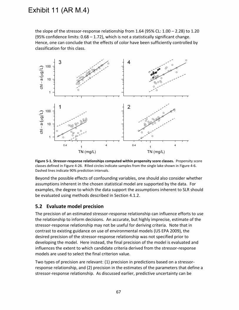
67
the slope of the stressor-response relationship from 1.64 (95% CL: 1.00 – 2.28) to 1.20 (95% confidence limits: 0.68 – 1.72), which is not a statistically significant change. Hence, one can conclude that the effects of color have been sufficiently controlled by classification for this class.
Figure 5-1. Stressor-response relationships computed within propensity score classes. Propensity score classes defined in Figure 4-26. Filled circles indicate samples from the single lake shown in Figure 4-6. Dashed lines indicate 90% prediction intervals.
Beyond the possible effects of confounding variables, one should also consider whether assumptions inherent in the chosen statistical model are supported by the data. For examples, the degree to which the data support the assumptions inherent to SLR should be evaluated using methods described in Section 4.1.2.
5.2 Evaluate model precision
The precision of an estimated stressor-response relationship can influence efforts to use the relationship to inform decisions. An accurate, but highly imprecise, estimate of the stressor-response relationship may not be useful for deriving criteria. Note that in contrast to existing guidance on use of environmental models (US EPA 2009), the desired precision of the stressor-response relationship was not specified prior to developing the model. Here instead, the final precision of the model is evaluated and influences the extent to which candidate criteria derived from the stressor-response models are used to select the final criterion value.
Two types of precision are relevant: (1) precision in predictions based on a stressor-response relationship, and (2) precision in the estimates of the parameters that define a stressor-response relationship. As discussed earlier, predictive uncertainty can be
Exhibit 11 (AR M.4)

68
quantified by examining the residual variance of an estimated regression relationship (i.e., the degree to which sample values are scattered around the mean relationship). When relationships are estimated across different waterbodies, this residual variance originates from both within- and across-site sources, and different interpretations of these two sources of uncertainty are appropriate. More specifically, within-site variability may not be relevant when deriving a candidate criterion because in many cases the goal is to maintain average conditions within a particular waterbody at a specified threshold. Conversely, uncertainty that can be attributed to across-site variability generally must be considered carefully to ensure that all waterbodies within a particular area support designated uses.
Large values of across-site variability can make it difficult to specify a single criterion because the criterion value may be too high for many waterbodies in the area to assure that it is appropriately protective for the most sensitive waterbodies. Consider, for example, the set of five lakes shown in Figure 4-8 (reproduced in Figure 5-2). For these lakes, a TN criterion value of 1.57 mg/L maintains an average chl a concentration of 20 μg/L or lower in the least sensitive lake (Arrow B). However, this TN criterion value is higher than is needed to protect the most sensitive lake. Indeed, setting the TN criterion value at 1.57 mg/L results in an average chl a concentration of 51 μg/L in the most sensitive lake (Figure 5-2). Average chl a concentrations in other lakes in the group would also exceed the desired threshold of 20 μg/L.
Figure 5-2. Illustration of range of chl a values associated with a selected criterion. Same data as Figure 4-8. Arrow B indicates TN criterion based on the least sensitive lake. Dashed arrow indicates prediction of mean chl a concentration at the most sensitive lake for this criterion value.
Conversely, a TN criterion value of 0.97 mg/L (Arrow A in Figure 4-8) would protect the most sensitive lake in the group, but would result in chl a concentrations that are substantially less than 20 μg/L in other lakes in the group.
Exhibit 11 (AR M.4)

69
The degree to which over- or under-protection of different waterbodies in a study area is acceptable, and by association, the acceptable precision of a stressor-response relationship, is ultimately a management decision. However, accurate estimates of within- and across-site variability for a particular stressor-response relationship are critical for informing this decision. In cases in which across-site variability is determined to be too large, further analysis and classification may be required to reduce this variability before a single criterion value can be determined.
In the example shown in Figure 5-1, the precision of the estimated stressor-response relationship varies across the different classes, and these differences in precision influence whether the estimated relationship can be usefully interpreted for deriving criteria. In Class 3, the width of the prediction intervals seems narrow enough such that a single criterion value could be applied to all lakes in this class. However, in other classes (e.g., Class 1) prediction intervals may be too wide to support a single criterion value. Data in these other classes are cases in which further classification and analyses may be useful. For example, the range of conductivity and color values associated with propensity score Class 1 is large (see Figure 4-26) and classes based on agglomerative clusters identify several different subclasses within Class 1 (compare Class 1 in Figure 4-26 with Classes 6 and 7 in Figure 4-25). If the classification scheme for Class 1 is refined and these subclasses are excluded, then the resulting precision of the stressor-response model improves substantially (Figure 5-3). Note that samples should not be excluded simply because they contribute to a large residual variability in the estimated stressor-response relationship. In the example shown here, values of covariates were evaluated separately from the estimate of the stressor-response relationship to identify subclasses.
Figure 5-3. Refinement of classification of sites for Class 1 (see Figure 5-1). Filled circles indicate sites that are excluded by classification refinement. Solid line and dashed lines indicate SLR fit and 90% prediction intervals for remaining sites in class.
Precision in the estimates of parameters that define the stressor-response relationship should also be evaluated with regard to informing decisions. This uncertainty can be evaluated by examining confidence intervals about estimated stressor-response
Exhibit 11 (AR M.4)

70
relationships (see for example, Figure 4-7). These confidence intervals indicate a range of values that the mean relationship could take, given the data. Broad confidence intervals indicate less certainty in predictions of average conditions. As discussed earlier, one appropriate interpretation of confidence intervals is to err toward a conservative, more protective criterion value.
5.3 Consider implementation issues
The primary implementation issue to consider at this stage is whether variables that are used to classify sites can also be used when developing water quality criteria. As discussed earlier, variables that quantify anthropogenic stressors or human activities, while particularly useful for helping to control for possible confounding effects, are generally not used to classify sites when developing criteria. Consequently, at this stage, the analyst must derive criteria that do not depend on anthropogenic stressors. Several solutions are possible.
First, if nutrient stressor-response relationships are similar across classes associated with different anthropogenic stressors, then one can combine these classes and eliminate the dependence on the anthropogenic stressor. For example, initial classification analysis might indicate that classifying by bedded sediment is necessary, but the slopes of the estimated stressor-response relationships are similar across all levels of bedded sediment. Thus, classes associated with different levels of bedded sediment can be combined and criteria derived that are independent of sediment.
Second, if nutrient stressor-response relationships differ across classes defined by anthropogenic stressors, one might estimate an average effect of nutrients across the entire data set by averaging the slopes of stressor-response relationships for the different classes. This average slope could then be used to derive criteria. Over the entire dataset, the average slope is a valid estimate of the overall effects of nutrients, but an obvious disadvantage of this approach is that differences in the effects of nutrients in different types of sites may not be accurately represented.
Third, it may be appropriate to specify different designated uses for different classes, and apply different stressor-response relationships for each class. For example, classification analyses may separate cold water from warm water streams in a particular region, and the designated uses for these two classes of streams may differ. Then, use of different stressor-response relationships and potentially different criteria for these two classes of streams may be appropriate.
Finally, in some cases one may be able to substitute a variable that quantifies a natural gradient for a variable that quantifies an anthropogenic stressor or human activity. For example, elevation is often strongly correlated with levels of bedded sediment and so, classifying sites by elevation may provide a similar degree of control for confounding as classifying by bedded sediment. Use of a natural gradient to classify sites eliminates the problem in which a nutrient criterion value would potentially depend upon the value of other stressors at a site.
Exhibit 11 (AR M.4)

71
5.4 Document analyses
Complete documentation of analyses is necessary so that others can evaluate the accuracy and precision of estimated stressor-response relationships and the defensibility of resulting criteria. The key elements of the analyses that should be documented are as follows: data, statistical analyses, and derived criteria.
The data on which the stressor-response analyses are built should be thoroughly documented. Information such as the sources of data, sampling design, sampling time, purposes of the data collection the collection methodologies, and the quality of data should be provided. Any relevant exploratory analyses that led to excluding particular samples or that informed subsequent formal statistical analysis should also be described.
Statistical analyses leading to the final estimated stressor-response relationships should be thoroughly documented. These analyses include the final classification approach, a priori and a posteriori evaluations of model accuracy, and final estimates of stressor-response relationships.
Finally, analysts should document the methods used to derive criteria from the estimated stressor-response relationships. The methods by which estimated stressor-response relationships are interpreted to yield numeric nutrient criteria should be thoroughly described.
If several different response variables have been analyzed, then the different candidate criteria derived for each variable should be compared and discussed. The relative precision and accuracy of stressor-response relationships used to derive different candidate criteria can be compared, and used qualitatively to weight different candidate criteria when selecting a final value. Also, candidate criteria derived using other methods (e.g., reference site distributions, literature values) can be compared qualitatively with criteria derived using stressor-response relationships.
Exhibit 11 (AR M.4)

72
6 References
Allan, J. D. and M. M. Castillo. 2007. Stream Ecology: Structure and Function of Running Waters. 2nd Edition. Springer.
Bennett, E. M., S. R. Carpenter, and N. F. Caraco. 2001. Human impact on erodable phosphorus and eutrophication: a global perspective. BioScience 51:227–234.
Biggs, B. J. F. 2000. Eutrophication of streams and rivers: dissolved nutrient–chlorophyll relationships for benthic algae. Journal of the North American Benthological Society 19:17–31.
Bothwell, M.L. 1985. Phosphorus limitation of lotic periphyton growth rates: an intersite comparison using continuous-flow troughs (Thompson River system, British Columbia). Limnology and Oceanography 30:527–542.
Bourassa, N., and A. Cattaneo. 1998. Control of periphyton biomass in Laurentian streams (Quebec). Journal of the North American Benthological Society 17:420–429.
Bowling, L.C., and P.D. Baker. 1996. Major cyanobacterial bloom in the Barwon-Darling River, Australia, in 1991, and underlying limnological conditions. Marine and Freshwater Research 47: 643–657.
Brenden, T.O., L. Wang, and Z. Su. 2008. Quantitative identification of disturbance thresholds in support of aquatic resource management. Environmental Management 42:821 – 832.
Breiman, L., J. H. Friedman, R. Olshen, and C. J. Stone. 1984. Classification and Regression Trees. Wadsworth International Group, Belmont, CA.
Cade, B.S. and B.R. Noon. 2003. A gentle introduction to quantile regression for ecologists. Frontiers in Ecology and the Environment 1:412 – 420.
Cade, B.S., J.W. Terrell, and R. L. Schroeder. 1999. Estimating effects of limiting factors with regression quantiles. Ecology 80:311–323.
Caraco N.F., J.J. Cole, S.F. Findlay, and K. Wigand. 2006. Vascular plants as engineers of oxygen in aquatic systems. Bioscience 56:221-225.
Carlson R.E. 1977. A trophic state index for lakes. Limnology and Oceanography 22:361 – 369.
Carpenter, S.R., N. F. Caraco, D. L. Correll, R. W. Howarth, A. N. Sharpley, and V. H. Smith. 1998. Nonpoint pollution of surface waters with phosphorus and nitrogen. Ecological Applications 8: 559–568.
Chapra, S.C. 1997. Surface Water-Quality Modeling, McGraw-Hill, New York, N.Y.
Cleveland, W. S. 1993. Visualizing Data. Summit, New Jersey, Hobart Press.
Exhibit 11 (AR M.4)

73
Cleveland, W. S., E. Grosse and W. M. Shyu. 1992. Local Regression Models. Statistical Models in S. J. H. Chambers and T. J. Hastie. Pacific Grove, CA, Wadsworth & Brook: 309 – 376.
Connell, J.H. and W.P. Sousa. 1983. On the evidence needed to judge ecological stability or persistence. American Naturalist 121: 789–824.
Correll, D. L. 1998. Role of phosphorus in the eutrophication of receiving waters: A review. Journal of Environmental Quality 27:261 – 266.
Cross, W. F., J. B. Wallace, A. D. Rosemond, and S. L. Eggert. 2006. Whole-system nutrient enrichment increases secondary production in a detritus-based ecoystem. Ecology 87: 1556–1565.
Cummins, K. W. and M. J. Klug. 1979. Feeding ecology of stream invertebrates. Annual Review of Ecology and Systematics 10:147–172.
Dake, J. M. and D. R. F. Harleman. 1969. Thermal stratification in lakes: analytical and laboratory studies. Water Resources Research 5:484 – 495.
Dillon, P. J. and F. H. Rigler. 1974. The phosphorus-chlorophyll relationship in lakes. Limnology and Oceanography 19: 767 – 773.
Dodds, W.K., and D.A. Gudder. 1992. The ecology of Cladophora. Journal of Phycology 28:415–427.
Downing, J. A. and E. McCauley. 1992. The nitrogen: phosphorus relationship in lakes. Limnology and Oceanography, 37:936 – 945.
Downing, J. A., S. B. Watson, and E. McCauley. 2001. Predicting cyanobacteria dominance in lakes. Canadian Journal of Fisheries and Aquatic Sciences 58: 1905–1908.
Dudley, T.L., S.D. Cooper, and N. Hemphill. 1982. Effects of macroalgae on a stream invertebrate community. Journal of the North American Benthological Society 5:93-106.
Dunne, T. and L.B. Leopold. 1978. Water in Environmental Planning. W.H. Freeman and Company. New York. pp. 818.
Elwood, J.W., J.D. Newbold, A.F. Trimble, AND R.W. Stark. 1981. The limiting role of phosphorus in a woodland stream ecosystem: effects of P enrichment on leaf decomposition and primary producers. Ecology 62:146–158.
Elser, J.J., M.E.S. Bracken, E.E. Cleland, D.S. Gruner, W.S. Harpole, H. Hillebrand, J.T. Ngai, E.W. Seabloom, J.B. Shurin, and J.E. Smith. 2007. Global analysis of nitrogen and phosphorus limitation of primary production in freshwater, marine, and terrestrial ecosystems. Ecology Letters 10: 1135-1142
Elser, J.J., E.R. Marzolf, and C.R. Goldman. 1990. Phosphorus and nitrogen limitation of phytoplankton growth in the freshwaters of North America: a review and
Exhibit 11 (AR M.4)

74
critique of experimental enrichments. Canadian Journal of Fisheries and Aquatic Science, 47, 1468–1477.
Feminella, J. W. and C. P. Hawkins. 1995. Interactions between stream herbivores and periphyton: A quantitative analysis of past experiments. Journal of the North American Benthological Society 14: 465–509.
Fisher, S. G. and G. E. Likens. 1973. Energy flow in Bear Brook, New Hampshire: an integrative approach to stream ecosystem metabolism. Ecological Monographs 43:421 – 439.
Francoeur, S.N. 2001. Meta-analysis of lotic nutrient amendment experiments: detecting and quantifying subtle responses. Journal of the North American Benthological Society 20: 358–368.
Fukami, T. and D. A. Wardle. 2005. Long-term ecological dynamics: reciprocal insights from natural and anthropogenic gradients. Proceedings of the Royal Society B: Biological Sciences 272: 2105 – 2115.
Fuller, R.L., J.L. Roelofs, and T.J. Fry. 1986. The importance of algae to stream invertebrates. Journal of North American Benthological Society 5: 290-296.
Gelman, A., J. B. Carlin, H. S. Stern, and D. R. Rubin. 2009. Bayesian Data Analysis 2nd Edition. Chapman & Hall/CRC, Boca Raton FL.
Gorham, E. and F. M. Boyce. 1989. Influence of lake surface area and depth upon thermal stratification and the depth of the summer thermocline Journal of Great Lakes Research, 15:233 – 245.
Gulis, V., A. D. Rosemond, K. Suberkropp, H. S. Weyers, and J. P. Benstead. 2004. Effects of nutrient enrichment on the decomposition of wood and associated microbial activity in streams. Freshwater Biology 49: 1437– 447.
Gulis, V., and K. Suberkropp. 2003. Leaf litter decomposition and microbial activity in nutrient-enriched and unaltered reaches of a headwater stream. Freshwater Biology 48:123 – 134.
Harrell Jr, F.E., K.L. Lee, and D.B. Mark. 1996. Multivariable prognostic models: issues in developing models, evaluating assumptions and adequacy, and measuring and reducing errors. Statistics in Medicine 28:361 – 387.
Hawkins, C. P., M. L. Murphy, and N. H. Anderson. 1982. Effects of canopy, substrate composition, and gradient on the structure of macro-invertebrate communities in Cascade Range streams of Oregon. Ecology 63:1840-1856.
Heiskary, S. and William W. Walker. 1988. Developing phosphorus criteria for Minnesota lakes. Lake and Reservoir Management 4:1 – 9.
Herlihy, A. T., S. G. Paulsen, J. Van Sickle, J. L. Stoddard, C. P. Hawkins, and L. L. Yuan. 2008. Striving for consistency in a national assessment: the challenges of
Exhibit 11 (AR M.4)

75
applying a reference-condition approach at a continental scale. Journal of the North American Benthological Society 27: 860 – 877.
Hill, W. R., M. G. Ryon, and E. M. Schilling. 1995. Light limitation in a stream ecosystem: responses by primary producers and consumers. Ecology 76: 1297 – 1309.
Hillebrand, H. 2002. Top-down versus bottom-up control of autotrophic biomass- A meta-analysis of experiments with periphyton. Journal of the North American Benthological Society 21: 349–369.
Horner, R.R., E.B. Welch, and R.B. Veenstra. 1983. Development of nuisance periphytic algae in laboratory streams in relation to enrichment and velocity. Pages 121–134 in R. G. Wetzel (editor). Periphyton of freshwater ecosystems. Dr. W. Junk Publishers, The Hague, The Netherlands.
Imai, K. and D. A. Van Dyk. 2004. Causal inference with general treatment regimes: Generalizing the propensity score. Journal of the American Statistical Association 99: 854–866.
Jeppesen, E., M. Søndergaard, J. P. Jensen, K. E. Havens, O. Anneville, L. Carvalho, E. F. Coveney, R. Deneke, M. T. Dokulil, B. Foy, D. Gerdeaux, S. E. Hampton, S. Hilt, K. Kangur, J. Köhler, E. H. H. R. Lammens, T. L. Lauridsen, M. Manca, M. R. Miracle, B. Moss, P. Nõges, G. Persson, G. Phillips, R. Portielje, S. Romo, C. L. Schelske, D. Straile, I. Tatrai, E. Willen, and M. Winder. 2005. Lake response to reduced nutrient loading – an analysis of contemporary long-term data from 35 case studies. Freshwater Biology 50: 1747 – 1771.
Jolliffe, I.T. 2002. Principal Components Analysis, 2nd edition. Springer, New York NY.
Jones, K. B., A. C. Neale, M. S. Nash, R. D. Van Remortel, J. D. Wickham, K. H. Riiters, and R. V. O’Neill. 2001. Predicting nutrient and sediment loadings to streams from landscape metrics: A multiple watershed study from the United States Mid-Atlantic Region. Landscape Ecology 16: 301 – 312.
Jongman, R. H., C. J. F. ter Braak, and O. F. R. Van Tongeren. 1995. Data Analysis in Community and Landscape Ecology. Cambridge University Press.
King, R.S. and C. J. Richardson. 2003. Integrating bioassessment and ecological risk assessment: an approach to developing numerical water-quality criteria. Environmental Management 31: 795 – 809.
Koenker, R. 2005. Quantile Regression. Cambridge University Press, Cambridge, UK.
Koenker, R. and G. Bassett, Jr. 1978. Regression Quantiles. Econometrica 46:33 – 50.
Koenker, R. and K.F. Hallock, 2001. Quantile Regression. Journal of Economic Perspectives 15:43 – 156.
Kutner, M. H., C. J. Nachtsheim, and J. Neter. 2004. Applied Linear Regression Models. McGraw-Hill/Irwin, Chicago, IL.
Exhibit 11 (AR M.4)

76
Lamon III, E.C. and S.S. Qian. 2008. Regional scale stressor-response models in aquatic ecosystems. Journal of the American Water Resources Association 44: 771–781.
Lee, G. F., W. Rast, R. A. Jones. 1978. Eutrophication of water bodies: Insights for an age-old problem. Environmental Science and Technology 12: 900 – 908.
May, R.M. 1977. Thresholds and breakpoints in ecosystems with a multiplicity of stable states. Nature 269: 471–77.
McCullagh, P. and J.A. Nelder. 1991. Generalized Linear Models, 2nd Edition. Monographs on Statistics and Applied Probability 37. CRC Press, Boca Raton, FL.
Miranda L. E., Driscoll M. P., Allen M. S. 2000. Transient physiochemical microhabitats facilitate fish survival in inhospitable aquatic plant stands. Freshwater Biology 44: 617–628.
Morgan, S. L. and C. Winship. 2007. Counterfactuals and Causal Inference. Cambridge University Press.
Moss, B., I. Hooker, H. Balls, and K. Manson. 1989. Phytoplankton distribution in a temperate floodplain lake and river system. I. Hydrology, nutrient sources and phytoplankton biomass. Journal of Plankton Research 11: 813–835.
Mulholland, P.J. and J.R. Webster. 2010. Nutrient dynamics in streams and the role of J-NABS. Journal of the North American Benthological Society 29: 100-117.
National Academy of Science. 1969. Eutrophication: Causes, Consequences, Correctives. National Academy of Science, Washington, DC.
Novotny, V. 2003. Water quality: Diffuse pollution and watershed management. 2nd edition. John Wiley & Sons, Inc. New York. pp. 864.
Odum, E.P., J.T. Finn, and E.H. Franz. 1979. Perturbation theory and the subsidy-stress gradient. Bioscience 29:344 – 352.
Omernik, J.M., S.S. Chapman, R.A. Lillie, and R.T. Dumke. 2000. Ecoregions of Wisconsin. Transactions of the Wisconsin Academy of Sciences, Arts and Letters 88:77 – 103.
Paerl, H.W. 1988. Nuisance phytoplankton blooms in coastal, estuarine, and inland waters. Limnology and Oceanography 33:823-847.
Pan, Y., R. J. Stevenson, P. Vaithiyanathan, J. Slate, and C. J. Richardson. 2000. Changes in algal assemblages along observed and experimental phosphorus gradients in a subtropical wetland, U.S.A. Freshwater Biology 44:339-353.
Paul, J. F. and M. E. McDonald. 2005. Development of empirical, geographically specific water quality criteria: A conditional probability analysis approach. Journal of the American Water Resources Association 41: 1211 – 1223.
Paul, M. J., and J. L. Meyer. 2001. Streams in the urban landscape. Annual Review of Ecology and Systematics 32: 333 – 365.
Exhibit 11 (AR M.4)

77
Pearl, J. 2009. Causality: Models, Reasoning, and Inference. Cambridge University Press, New York.
Peterson, B.J., J.E. Hobbie, A.E. Hershey, M.A. Lock, T.E. Ford, J.R. Vestal, V.L. McKinley, M.A.J. Hullar, M.C. Miller, R.M. Ventullo, and G. S. Volk. 1985. Transformation of a tundra river from heterotrophy to autotrophy by addition of phosphorus. Science 229:1383–1386.
Philips, E. J., M. Cichra, F. J. Aldridge, J. Jembeck, J. Hendrickson, and R. Brody. 2000. Light availability and variations in phytoplankton standing crops in a nutrient-rich blackwater river. Limnology and Oceanography 45: 916 – 929.
Pielou, E. C. 1984. The interpretation of ecological data: A primer on classification and ordination. John Wiley and Sons, New York.
Pinheiro, J. C. and D. M. Bates. 2000. Mixed-Effects Models in S and S-Plus. Springer. New York, NY.
Proschan, F. 1953. Confidence and tolerance intervals for the normal distribution. Journal of the American Statistical Association 48:550 – 564.
Qian, S.S., R. S. King, and C.J. Richardson. 2003. Two statistical methods for the detection of environmental thresholds. Ecological Modeling 166: 87–97.
Reckhow, K.H. 1979. Uncertainty analysis applied to Vollenweider phosphorus loading criterion. Journal of the Water Pollution Control Federation 51: 2123-2128.
Reckhow, K.H., G.B. Arhonditsis, M.A. Kenney, L. Hauser, J. Tribo, C. Wu, L.J. Steinberg, C. A. Stow, and S. J. McBride. 2005. A Predictive Approach to Nutrient Criteria. Environmental Science and Technology. 39: 2913 – 2919.
Rosemond, A. D., P. J. Mulholland, and J. W. Elwood. 1993. Top-down and bottom-up control of stream periphyton: Effects of nutrients and herbivores. Ecology 74: 1264–1280.
Rosemond, A. D., C. M. Pringle, A. Ramirez, and M.J. Paul. 2001. A test of top-down and bottom-up control in a detritus-based food web. Ecology 82: 2279–2293.
Rosemond, A. D., C. M. Pringle, A. Ramirez, M.J. Paul, and J. L. Meyer. 2002. Landscape variation in phosphorus concentration and effects on detritus-based tropical streams. Limnology and Oceanography 47: 278–289.
Rosenbaum, P.R. 2002. Observational Studies, 2nd Edition. Springer, New York.
Rosenbaum, P.R. and D. B. Rubin. 1983. The central role of the propensity score in observational studies for causal effects. Biometrika 70: 41–55.
Rothman, K.J., S. Greenland, and T. L. Roth. 2008. Modern Epidemiology. Lippincott Williams & Wilkins. Philadelphia, PA.
Rubin, D. B. and R. J. A. Little. 2002. Statistical analysis with missing data, 2nd edition. Wiley, New York, NY.
Exhibit 11 (AR M.4)

78
Scheffer, M., D. Straile, E.H. van Nes, and H. Hosper. 2001. Climatic warming causes regime shifts in lake food webs. Limnology and Oceanography 46: 1780–83.
Schindler D.W. 1974. Eutrophication and recovery in experimental lakes: Implications for lake management. Science 184:897–899.
Schindler D.W., H. Kling, R.V. Schmidt, J. Prokopowich, V.E. Frost, R. A. Reid, and M. Capel. 1973. Eutrophication of Lake 227 by addition of phosphate and nitrate: The second, third, and fourth years of enrichment 1970, 1971, and 1972. Journal of the Fishery Research Board of Canada 30:1415–1440.
Schindler, D.W., R.E. Hecky, D.L. Findlay, M.P. Stainton, B.R., Parker, M.J. Paterson, K.G. Beaty, M. Lyng, and S.E.M. Kasian. 2008. Eutrophication of lakes cannot be controlled by reducing nitrogen input: Results of a 37-year whole-ecosystem experiment. Proceedings of the National Academy of Sciences 105:11254-11258.
Slavik, K., B. J. Peterson, L. A. Deegan, W. B. Bowden, A. E. Hershey, and J. E. Hobbie. 2004. Long-term responses of the Kuparuk River ecosystem to phosphorus fertilization. Ecology 85: 939 – 954.
Smil, V. 2000. Phosphorus in the environment: natural flows and human interferences. Annual Review of Energy and the Environment 25:53–88.
Smith, V.H. 1979. Nutrient dependence of primary productivity in lakes. Limnology and Oceanography, 24: 1051 – 1064.
Smith, V.H. 1982. The nitrogen and phosphorus dependence of algal biomass in lakes: An empirical and theoretical analysis. Limnology and Oceanography, 27: 1101 – 1112.
Smith, V.H. 1998. Cultural eutrophication of inland, estuarine, and coastal waters. In: Pace, M.L., Groffman, P.M. (eds) Successes, Limitations and Frontiers in Ecosystem Sciences. Springer, New York. pp. 7-49.
Smith, V.H. 2003. Eutrophication of freshwater and coastal marine ecosystems: A global problem. Environmental Science and Pollution Research 10: 126 – 139.
Smith, V.H., S.B. Joye, and R.W. Howarth. 2006. Eutrophication of freshwater and marine ecosystems. Limnology and Oceanography 51: 351-355.
Smith, V.H., G.D. Tilman, and J.C. Nekola. 1999. Eutrophication: impacts of excess nutrient inputs on freshwater, marine, and terrestrial ecosystems. Environmental Pollution 100, 179–196.
Stockner, J.G., and K.R.S. Shortreed. 1976. Autotrophic production in Carnation Creek, a coastal rainforest stream on Vancouver Island, British Columbia. Journal of the Fisheries Research Board of Canada 33:1553–1563.
Stockner, J.G., and K.R.S. Shortreed. 1978. Enhancement of autotrophic production by nutrient addition in a coastal rainforest stream on Vancouver Island. Journal of the Fisheries Research Board of Canada 35:28–34.
Exhibit 11 (AR M.4)

79
Stoddard, J. L., D. P. Larsen, C. P. Hawkins, R. K. Johnson, and R. H. Norris. 2006a. Setting expectations for the ecological condition of streams: the concept of reference condition. Ecological Applications 16:1267 – 1276.
Stoddard, J. L., D. V. Peck, A. R. Olsen, D. P. Larsen, J. Van Sickle, C. P. Hawkins, R. M. Hughes, T. R. Whittier, G. Lomnicky, A. T. Herlihy, P. R. Kaufmann, S. A. Peterson, P. L. Ringold, S. G. Paulsen, and R. Blair. 2006b. Environmental Monitoring and Assessment (EMAP) western streams and rivers statistical summary. EPA/620/R-05/006. Office of Research and Development, US Environmental Protection Agency, Washington, DC.
Stoddard, J.L, A.T. Herlihy, D.V. Peck, R.M. Hughes, T.R. Whittier, and E. Tarquinio. 2008. A process for creating multimetric indices for large-scale aquatic surveys. Journal of the North American Benthological Society 27:878 – 891.
Suplee, M.W., V. Watson, M. Tepley, and H. McKee. 2009. How Green is Too Green? Public Opinion of What Constitutes Undesirable Algae Levels in Streams. Journal of the American Water Resources Association 45: 123–140
Tukey, J. W. 1977. Exploratory Data Analysis. Reading, Massachusetts, Addison-Wesley Publishing Co.
US EPA. 1985. Guidelines for Deriving Numerical National Water Quality Criteria for the Protection of Aquatic Organisms and their Uses. PB85-227049. National Technical Information Service. Springfield, VA.
US EPA. 1986. Quality Criteria for Water 1986. EPA 440/5-86-001. U.S. Environmental Protection Agency, Office of Water, Washington, D.C.
US EPA. 1998. Guidelines for Ecological Risk Assessment. Risk Assessment Forum. Washington DC. EPA/630/R-95/002F.
US EPA. 2000a. Nutrient Criteria Technical Guidance Manual: Rivers and Streams. EPA-822-B-00-002. U.S. Environmental Protection Agency, Office of Water, Washington, D.C.
US EPA. 2000b. Nutrient Criteria Technical Guidance Manual. Lakes and Reservoirs. EPA-822-B-00-001. U.S. Environmental Protection Agency, Office of Water, Washington, DC.
US EPA. 2001. Nutrient Criteria Technical Guidance Manual. Estuarine and Coastal Marine Waters. EPA-822-B-01-003. U.S. Environmental Protection Agency, Office of Water, Washington, DC.
US EPA. 2006. Data Quality Assessment: A Reviewer’s Guide. Office of Environmental Information. Washington, DC. EPA/240/B-06/002.
US EPA. 2008. Nutrient Criteria Technical Guidance Manual. Wetlands. EPA-822-B-08-001. U.S. Environmental Protection Agency, Office of Water, Washington, DC.
Exhibit 11 (AR M.4)

80
US EPA. 2009. Guidance on the Development, Evaluation, and Application of Environmental Models. Office of the Science Advisor, Council for Regulatory Environmental Modeling. Washington, DC. EPA/100/K-09/003.
US EPA. 2010. Causal Analysis Decision Diagnosis Information System (CADDIS). Office of Research and Development, Washington DC. http://www.epa.gov/caddis/.
Vannote, R. L., G. W. Minshall, K. W. Cummins, J. R. Sedell, and C. E. Cushing. 1980. The river continuum concept. Canadian Journal of Fisheries and Aquatic Sciences 37:130 – 137.
Vardeman, S. B. 1992. What about other intervals? The American Statistician 46:193 – 197.
Venables, W. N. and B. D. Ripley. 2002. Modern Applied Statistics with S, 4th Edition. Springer.
Vitousek, P. M., J. D. Aber, R. W. Howarth, G. E. Likens, P. A. Matson, D. W. Schindler, W. H. Schlesinger, and D. G. Tilman. 1997. Human alteration of the global nitrogen cycle: sources and consequences. Ecological Applications 7:737–750.
Vollenweider, R.A. 1968. Scientific Fundamentals of the Eutrophication of Lakes and Flowing Waters, with Particular Reference to Nitrogen and Phosphorus as Factors in Eutrophication (Tech Rep DAS/CS/68.27, OECD, Paris).
Vollenweider, R.A. 1976. Advances in Defining Critical Loading Levels for Phosphorus in Lake Eutrophication. Memorie dell'Istituto Italiano di Idrobiologia 33:53 – 83.
Wallace, J.B. and M. E. Gurtz. 1986. Response of Baetis mayflies (Ephemeroptera) to catchment logging. American Midlands Naturalist 115:25-41.
Wetzel, R.G. 2001. Limnology—Lake and River Ecosystems, 3rd Edition. Academic Press. New York, N.Y.
Wilk, M. B. and R. Gnanadesikan. 1968. Probability Plotting Methods for the Analysis of Data. Biometrika 55: 1 – 17.
Wood, S. N. and N. H. Augustin. 2002. GAMs with integrated model selection using penalized regression splines and applications to environmental modelling. Ecological Modelling 157: 157– 77.
World Health Organization (WHO). 2003. Guidelines for Safe Recreational Water Environments, Volume 1: Coastal and Fresh Waters. World Health Organization, Geneva, Switzerland.
Exhibit 11 (AR M.4)