using svd for improved interferometric green™s function...

Using SVD for improved interferometric Green’s function recovery.Gabriela Melo∗1, Alison Malcolm1, Dylan Mikessel2, and Kasper van Wijk2

1Earth Resources Laboratory - Earth, Atmospheric, and Planetary Sciences Department - Massachusetts Institute of Technology2Physical Acoustic Lab - Department of Geosciences - Boise State University

SUMMARY

Seismic interferometry is a technique used to estimate theGreen’s function (GF) between two receiver locations, as ifthere were a source at one of the locations. By crosscorrelatingthe recorded seismic signals at the two locations we generate acrosscorrelogram. Stacking the crosscorrelogram over sourcesgenerates an estimate of the inter-receiver GF. However, inmost applications, the requirements to recover the exact GFare not satisfied and stacking the crosscorrelograms yields apoor estimate of the GF. For these non-ideal cases, we enhancethe real events in the virtual shot gathers by applying Singu-lar Value Decomposition (SVD) to the crosscorelograms be-fore stacking. The SVD approach preserves energy that is sta-tionary in the crosscorrelogram, thus enhancing energy fromsources in stationary positions, which interfere constructively,and attenuating energy from non-stationary sources that inter-fere distructively. We apply this method to virtual gathers con-taining the virtual refraction artifact and find that using SVDenhances physical arrivals. We also find that SVD is quite ro-bust in recovering physical arrivals from noisy data when thesearrivals are obscured by or even lost in the noise in the standardseismic interferometry technique.

INTRODUCTION

Seismic Interferometry (SI), first envisioned by Claerbout (1968),estimates the Green’s function (GF) between two receivers.This technique, often referred to as the virtual source methodin exploration seismology (Bakulin and Calvert, 2006), requiresthat the sources completely surround the receivers (Wapenaarand Fokkema, 2006). This assumption is rarely met in practiceand results in a degradation in the quality of the recovered GF.To overcome this problem, we study the collection of cross-correlated traces from many sources for a pair of receivers,referred to as a crosscorrelogram. Crosscorrelograms containpre-stack information, e.g., high frequency data that is oftenlost during stacking. Therefore, it is natural to expect that wecan extract parameters of interest from the crosscorrelogram.

We filter the crosscorrelograms using the singular value de-composition (SVD) (see e.g. Hansen (1999)), a numericaltechnique commonly used in seismic data processing (Ulrychet al., 1988; Sacchi et al., 1998), with the goal of enhancingevents that are coherent across multiple sources, i.e. stationaryenergy. Hansen et al. (2006) showed the relationship betweensingular values and frequency – larger singular values corre-spond to lower frequencies and smaller singular values corre-spond to higher frequencies. We apply SVD to crosscorrelo-grams, relying on the fact that signal due to stationary sources

occurs at low spatial frequency (in the source coordinate) andsignal from non-stationary sources (and random noise) gener-ally occurs at higher spatial frequencies. After decomposingthe crosscorrelogram into components that depend on spatialfrequency, we expect the signal from stationary sources to cor-respond to large singular values (i.e., low spatial frequency).Thus, we decompose the crosscorrelogram using SVD, con-struct a lower-rank approximation of the crosscorrelograms,using only the largest singular values, and stack the lower-rankcrosscorrelogram to estimate the GF. This approach recoversthe correct GF using fewer sources than required in the stan-dard SI technique.

Mikesell et al. (2009) showed that in shot gathers estimatedusing SI (i.e., virtual shot gathers) in a two-layered model withhead waves, an artifact arises from the crosscorrelation of headwaves recorded at the two receivers. They call this artifact thevirtual refraction. Rather than trying to suppress this artifact,they showed that it can be used to estimate the depth to theinterface and the velocity in the model layers. The real headwave, also present in the virtual shot gather, contains this in-formation as well. However, they showed that its amplitude isconsiderably weaker than the virtual refraction, making the lat-ter easier to interpret. We apply the SVD technique describedabove to the same synthetic data set used by Mikesell et al.(2009) in an attempt to further enhance the virtual refraction.We find instead that SVD enhances the real head wave. Wealso find that applying SVD to a noisy version of this data setenhances the reflected wave, even when it is almost completelyobscured by noise in the standard virtual shot gather.

THEORY

Wapenaar and Fokkema (2006) showed that the exact Green’sfunction between two receivers at locations xA and xB can berepresented by the integral over sources distributed throughouta closed surface surrounding the two receivers,

G(xA, xB , ω) + G∗(xA, xB , ω)

=

IS

−1

iωρ(x)(∂iG(xB , x, ω)G∗(xA, x, ω)

− G(xB , x, ω)∂iG∗(xA, x, ω))nidS , (1)

where G(xA, xB , ω) is the frequency domain GF for a re-ceiver at xA and a source at xB corresponding the to causalGF in the time domain, G∗(xA, xB , ω) is the complex conju-gate GF corresponding to the anti-causal GF in the time do-main, ρ(x) is the density, ω is the angular frequency, i =p

(−1), and S is the closed surface of sources surrounding thereceivers. We recall that the physical interpretation of ∂iG(xA, x, ω)is as the GF from a dipole source at x recorded at xA andG(xA, x, ω) is the GF from a monopole source at x recorded

3986SEG Denver 2010 Annual Meeting© 2010 SEG

Downloaded 05 Nov 2011 to 72.93.188.223. Redistribution subject to SEG license or copyright; see Terms of Use at http://segdl.org/

Improving interferometric GF using SVD.

at xA. Wapenaar and Fokkema (2006) simplify equation 1 bymaking the following assumptions: 1) all sources lie in thefar-field (i.e., the distance from the source to the receivers andscatterers is large compared to the wavelength); 2) rays takeoff approximately normal from the integration surface S; 3)the medium outside the integration surface S is homogeneous,such that no energy going outward from the surface is scat-tered back into the system; 4) the medium around the sourceis locally smooth (the high frequency approximation). Withthese assumptions, the spatial derivative is approximated asni∂iG ≈ (iωG)/c(x) in equation 1, which simplifies to

G(xA, xB , ω) + G∗(xA, xB , ω)

≈I

S

−2iωG(xB , x, ω)G∗(xA, x, ω)

ρ(x)c(x)dS . (2)

We now have an equation for crosscorrelation SI that requiresonly monopoles sources. In general, we only have monopoleseismic sources; therefore, equation 2 is used in the SI methodand the amplitudes of the GF are lost.

We now explore decomposing the crosscorrelogram using SVD.Consider a matrix A such that each column of A correspondsto a crosscorrelated trace for one source. Then A = A(t, s)is the crosscorrelogram. Suppose ns is the number of sources,nt is the number of time samples, t is time, s is the source,e = (1, ..., 1) is the ns × 1 vector with of ones, b = b(t)is the GF (i.e., the stack of the crosscorrelogram A along thesource dimension).

Using this notation, the stack of the crosscorrelogram is

Ae = b . (3)

Consider the SVD decomposition of the crosscorrelogram ma-trix A

A = UΣV t , (4)

where U is the orthonormal nt × nt matrix of left singularvectors (a basis for the columns of A), Σ is the nt×ns diagonalmatrix whose elements are the singular values of A, and V isthe orthonormal ns × ns right singular vector matrix (a basisfor the rows of A).

We can use the SVD decomposition to express the GF. Stack-ing A over the source dimension we get

Ae = UΣV te = b . (5)

We call Σ′ the reduced Σ matrix, containing only the largestsingular values. Then we construct a lower-rank approxima-tion of the crosscorrelogram

A′e = UΣ′V te = b′, (6)

where b′ is the approximate GF.

To illustrate this idea, consider the source-receiver geometry ina constant velocity/density medium, figure 1. The sources di-rectly to the left and right of the receivers are in the stationaryregion, and the sources above and below are in non-stationaryregions (Snieder, 2004). The gaps in sources break the require-ment of a closed surface S in equation 2, i.e. that the receivers

are completely surrounded by sources. In our numerical mod-eling we use 13 sources in each of the stationary zones and ninesources in each of the non-stationay zones. We used a Rickerwavelet as our source function and all receiver data are mod-eled analytically. Figure 2(a) shows the standard crosscorrel-ogram as well as the standard stack, figure 2(c), estimated bystacking the crosscorrelogram over source azimuth. The stan-dard crosscorrelogram contains energy from stationary sourcesthat contribute to the real GF and residual energy from non-stationary sources that causes artifacts due to incomplete can-cellation. The rank-2 crosscorrelogram, figure 2(b), and cor-responding GF, figure 2(d), are free from the non-stationaryenergy and fluctuations. We thus conclude that in this exam-ple, using SVD leads to a more accurate estimate of the GF.Next we show a more realistic 2D acquisition and discuss theapplication of SVD to a situation with multiple wave modes.

Figure 1: Source-receiver geometry for homogeneous model.

Figure 2: Standard (a) and rank-2 crosscorrelograms (b) andcorresponding GFs (c, d) for the source-receiver geometryshown in figure 1. The blue lines are the recovered GFs andthe red lines are the causal part of exact GFs for comparison.

EXAMPLES

We now apply the SVD technique discussed above to the samesynthetic data set used by Mikesell et al. (2009). Considerthe 2-layer acoustic model shown in figure 3. The top layerhas velocity V0 = 1250m/s, the bottom layer has velocityV1 = 1750m/s, and density is constant throughout the model.We attempt to create a virtual shot gather as if there were asource at receiver r1 using SI. Figure 4 shows the real shotgather for comparison. Note the direct, reflected, and refractedwaves present in the ‘real’ shot gather.

A 2D array of 110 sources is placed to the left of the receiverline (figure 3), resembling a standard 2D off-end seismic sur-vey. The wavefield generated by each source is recorded at




Figure 3: Virtual refraction source-receiver geometry.

Figure 4: Modeled shot gather with a source placed at the lo-cation of receiver r1. We have convolved the real shot gatherwith the 40 Hz Ricker wavelet used as a source.

each receiver. The GF between r1 and each of the other re-ceivers is obtained using crosscorrelation SI.

Figure 5(a)-(b) shows the standard and the rank-1 crosscorrel-ograms for receivers r1 and r18. Figure 5(c)-(d) shows thecausal part of the corresponding GF estimates in blue and theexact GF in red. The phase difference between the estimateand the exact GF’s is caused by the approximation to the closedsurface integral over S. The amplitude of the reflected arrival,relative to that of the direct arrival is more accurately recoveredusing the rank-1 approximate crosscorrelogram.

Figure 5: Standard (a) and rank-1 (b) crosscorrelograms andcorresponding GFs (c, d) for receivers r1 and r18.

Repeating this procedure for all receivers, we create a standardvirtual shot gather, figure 6, and a rank-1 shot gather, figure 7,for a virtual source at r1. As is expected from the results infigure 5, the rank–1 approximation has better recovered the re-

flected wave than in the standard virtual shot record. In addi-tion, the real refracted wave is clearer in the rank-1 approxima-tion than in the standard virtual shot gather. Each trace in theshot records (real and virtual) are normalized individually suchthat all direct arrivals have a peak amplitude of 1. All gathersare displayed with the same clipping; they are clipped to showthe weaker arrivals we are attempting to enhance. However,this means that geometrical spreading, or any other offset de-pendent amplitudes in general, will be lost. Also, as is standardin SI, we do not recover the exact amplitudes due to the lackof dipole sources in the approximate equation 1.

Figure 6: Interferometric virtual shot record for virtual sourceat r1. See Mikesell et al. (2009) figure 4(a). We recover all theevents in figure 4, plus the virtual refraction.

Figure 7: Rank-1 virtual shot gather. The real events are en-hanced when this shot gather is compared to figure 6.

We now add pseudo-random noise to the data before crosscor-relation to test the SVD method’s robustness in the presenceof noise. Figure 8 shows the real shot gather plus noise. Fig-ures 9(a)-(b) show again the standard and rank-1 crosssorrelo-grams for r1 and r18. Figures 9(c)-(d) show the respective GFestimates in blue and the exact GFs in red. We again see thatthe reflected wave GF amplitude is more accurately recoveredusing the rank-1 crosscorrelogram.

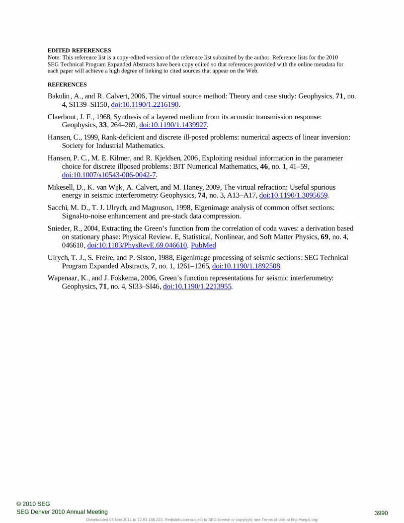
In the standard , figure 10, and in the rank-1 virtual shot gather,figure 11, we see that the rank-1 shot gather has recovered thereflected wave even though it is nearly obscured by noise in




the standard shot record. We also see some energy from thereal refracted wave in the rank-1 shot gather, whereas in thestandard shot gather this arrival is completely lost in the noise.

Figure 8: Modeled shot gather, similar to figure 4, but withadded noise.

Figure 9: Standard and rank-1 crosscorrelograms and GFs,similar to figure 5. Noise has been added to the synthetic dataso that the reflection and refraction are difficult to see in thestandard virtual shot gather.

CONCLUSIONS

An outstanding problem in seismic interferometry remains theaccurate estimation of the GF when the source coverage is notideal. We have shown theoretically why using SVD to ap-proximate crosscorrelograms before stacking is a promisingapproach to alleviate this problem. From the examples shown,we conclude that the rank-1 approximation of the correlogramhighlights reflected and refracted arrivals that are not properlyrecovered using the standard crosscorrelogram. In addition,we find that SVD is able to enhance arrivals that would oth-erwise be obscured by noise. Future directions include us-ing SVD on real data and to separate multiply-scattered signalfrom singly scattered signal in the crosscorrelogram as wellas using the covariance of the correlogram to locate stationarypoints necessary, for example, to estimate the depth of a layerfrom the virtual refraction.

Figure 10: Standard virtual shot gather, similar to figure 6, butwith added noise.

Figure 11: Rank-1 virtual shot gather with added noise. Notethe enhanced reflected wave compared to the reflected wavein the standard virtual shot gather in figure 10. Some of thephysical refraction energy is recovered here while it is lost instandard virtual gather.



EDITED REFERENCES Note: This reference list is a copy-edited version of the reference list submitted by the author. Reference lists for the 2010 SEG Technical Program Expanded Abstracts have been copy edited so that references provided with the online metadata for each paper will achieve a high degree of linking to cited sources that appear on the Web. REFERENCES

Bakulin, A., and R. Calvert, 2006, The virtual source method: Theory and case study: Geophysics, 71, no. 4, SI139–SI150, doi:10.1190/1.2216190.

Claerbout, J. F., 1968, Synthesis of a layered medium from its acoustic transmission response: Geophysics, 33, 264–269, doi:10.1190/1.1439927.

Hansen, C., 1999, Rank-deficient and discrete ill-posed problems: numerical aspects of linear inversion: Society for Industrial Mathematics.

Hansen, P. C., M. E. Kilmer, and R. Kjeldsen, 2006, Exploiting residual information in the parameter choice for discrete illposed problems: BIT Numerical Mathematics, 46, no. 1, 41–59, doi:10.1007/s10543-006-0042-7.

Mikesell, D., K. van Wijk, A. Calvert, and M. Haney, 2009, The virtual refraction: Useful spurious energy in seismic interferometry: Geophysics, 74, no. 3, A13–A17, doi:10.1190/1.3095659.

Sacchi, M. D., T. J. Ulrych, and Magnuson, 1998, Eigenimage analysis of common offset sections: Signal-to-noise enhancement and pre-stack data compression.

Snieder, R., 2004, Extracting the Green’s function from the correlation of coda waves: a derivation based on stationary phase: Physical Review. E, Statistical, Nonlinear, and Soft Matter Physics, 69, no. 4, 046610, doi:10.1103/PhysRevE.69.046610. PubMed

Ulrych, T. J., S. Freire, and P. Siston, 1988, Eigenimage processing of seismic sections: SEG Technical Program Expanded Abstracts, 7, no. 1, 1261–1265, doi:10.1190/1.1892508.

Wapenaar, K., and J. Fokkema, 2006, Green’s function representations for seismic interferometry: Geophysics, 71, no. 4, SI33–SI46, doi:10.1190/1.2213955.



using svd for improved interferometric green™s function...

Documents