using synthetic data to test downscaling methods john lanzante (gfdl/noaa)
TRANSCRIPT

Using Synthetic Data to Test Downscaling Methods
John Lanzante (GFDL/NOAA)

CONCEPTS
Testing Downscaling:
Like Product Testing
My Product

STEP1: Recruit Test Subjects (Gather Data)CONCEPTS
STEP2: Feed Cereal For Several Decades (Apply Downscaling Method)

CONCEPTS
STEP3: How are subjects affected? How well did downscaling do?
Not so clear – Need more subjects?
Need more data?
Real-world data may be limited?
Can we generate synthetic data to fill the void?

CONCEPTS
STEP 4a: Snowmen most affected? Generate a new sample.

CONCEPTS
STEP 4b: Snow-women affected differently? Generate a new sample.
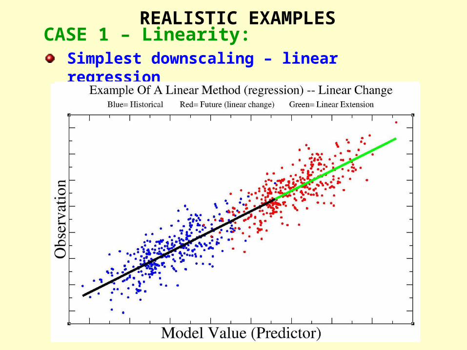
REALISTIC EXAMPLES
CASE 1 – Linearity:Simplest downscaling – linear regression

REALISTIC EXAMPLES
CASE 1 – Strong Nonlinearity:Simplest downscaling – linear regression

REALISTIC EXAMPLESSUMMARY CASE 1 – Nonlinearity:
Hard to test nonlinearity in real-world data ? (if we are just entering “non-linear regime”)
Simulate various degrees of nonlinearity
Compare linear & nonlinear downscaling methods
Determine amount of degradation
Determine time in future when degradation becomes “too large”

REALISTIC EXAMPLES
CASE 2 – Coastal Error:Downscaling error maximizes along coastline

REALISTIC EXAMPLESCASE 2 – Coastal Error:
Obs gridpoint Entirely land
Model gridpoint Partly land, partly ocean

REALISTIC EXAMPLESCASE 2 – Coastal Error:
Land more detail (extremes) than Ocean (damped)
Missing peaks & troughs unrecoverable

REALISTIC EXAMPLES
SUMMARY CASE 2 – Costal Error:
Simulate land & ocean points
Downscale land from mixture (land + sea)
Vary the proportions of the mixtureIs coastal effect due to mixture/mismatch?

SYNTHETIC DATA MODELOne Particular Synthetic Data Model: O= Observations M= Model y= year d= day Red = free parameter (user selects the value)
Oy d = Ōy + O’y d Yearly mean + AR1
O’y d = rlag1 * O’
y d-1 + ay d AR1
fvar = varŌ / varO [ varO = varŌ + varO]
My d = Oy d + by d corr = correlation(O,M)
a ~ N(0,vara) Proper choice of a & b b ~ N(0,varb) yields desired rlag1 & corr

SYNTHETIC DATA MODEL
STEP 1: Generate Base Time Series rlag1 day-to-day persistence fvar interannual vs. day-to-day variability corr strength of relation: model vs. obs
STEP 2: Historical Adjustment meanOBS characteristics of the distribution
meanMODEL
varOBS
varMODEL
STEP 3: Future Adjustment meanOBS characteristics of the distribution meanMODEL
varOBS
varMODEL

SYNTHETIC DATA MODEL
OUR APPLICATIONS OF THIS MODEL:
Downscaling (just getting started)
No results yet
Applied successfully to several related
issues (cross-validation, exceedance
statistics, testing two distributions)

SUMMARY
REAL-WORLD COMPLICATIONS:Results may not be clear-cut:
Sample size too small?
Multiple factors may contribute?
Some conditions more interesting?
SOLUTION – GENERATE SYNTHETIC DATA:
Advantages of Synthetic Data:Unlimited sample size (enhance signal/noise)
Change one factor at a time
Prescribe exact conditions
Vary factor over a wide range (“turn the knob”)
Can extend outside the range of historical data
Turn knob “all the way” for unambiguous results
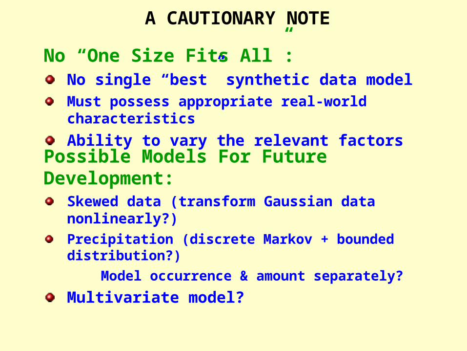
A CAUTIONARY NOTE
No “One Size Fits All”:No single “best” synthetic data modelMust possess appropriate real-world characteristics
Ability to vary the relevant factors
Possible Models For Future Development:Skewed data (transform Gaussian data nonlinearly?)
Precipitation (discrete Markov + bounded distribution?)
Model occurrence & amount separately?
Multivariate model?

THE END

REALISTIC EXAMPLES
CASE 1 – Weak Nonlinearity:Simplest downscaling – linear regression

SUPPLEMENTAL
Causes of Nonlinearity?
At highest T – model soil becomes excessively dry – T becomes excessiveOther possibilities: Water Vapor, Clouds, Sea-Ice, etc.

REALISTIC EXAMPLESCASE 2 – Coastal Error:
Land More extremes
Ocean Damped

REALISTIC EXAMPLES
CASE 2 – Coastal Error:X/Y Plot: Land (model) vs. Land (obs)

REALISTIC EXAMPLES
CASE 2 – Coastal Error:X/Y Plot: Ocean (model) vs. Land (obs)

SYNTHETIC DATA MODEL
STEP 4:Fit downscaling model to historical sample
STEP 5:Test downscaling in historical & future samples
OUR APPLICATIONS OF THIS MODEL:No results to show today
Downscaling (just getting started)
Guidance in the use of cross-validation
Biases in exceedance statistics
Testing difference between 2 distributions