using temporal variability to improve spatial mapping with application to satellite data

The Canadian Journal of StatisticsVol. 38, No. 2, 2010, Pages 271–289La revue canadienne de statistique

271

Using temporal variability to improve spatialmapping with application to satellite dataEmily L. KANG, Noel CRESSIE* and Tao SHI

Department of Statistics, The Ohio State University, Columbus, OH 43210-1247, USA

Key words and phrases: Aerosol Optical Depth (AOD); fine-scale variability; Fixed Rank Filtering (FRF);Fixed Rank Kriging (FRK); Multi-angle Imaging SpectroRadiometer (MISR) instrument; Spatial RandomEffects (SRE)model; Spatio-TemporalRandomEffects (STRE)model; vector autoregressive (VAR) process.

MSC 2000: Primary 62P12; secondary 62M30.

Abstract: The National Aeronautics and Space Administration (NASA) has a remote-sensing program witha large array of satellites whose mission is earth-system science. To carry out this mission, NASA producesdata at various levels; level-2 data have been calibrated to the satellite’s footprint at high temporal resolution,although there is often a lot of missing data. Level-3 data are produced on a regular latitude–longitude gridover the whole globe at a coarser spatial and temporal resolution (such as a day, a month, or a repeat-cycle ofthe satellite), and there are still missing data. This article demonstrates that spatio-temporal statistical modelscan be made operational and provide a way to estimate level-3 values over the whole grid and attach to eachvalue a measure of its uncertainty. Specifically, a hierarchical statistical model is presented that includesa spatio-temporal random effects (STRE) model as a dynamical component and a temporally independentspatial component for the fine-scale variation. Optimal spatio-temporal predictions and their mean squaredprediction errors are derived in terms of a fixed-dimensional Kalman filter. The predictions provide estimatesof missing values and filter out unwanted noise. The resulting fixed-rank filter is scalable, in that it can handlevery large data sets. Its functionality relies on estimation of the model’s parameters, which is presented in de-tail. It is demonstrated howboth past and current remote-sensing observations on aerosol optical depth (AOD)can be combined, yielding an optimal statistical predictor of AOD on the log scale along with its predictionstandard error. The Canadian Journal of Statistics 38: 271–289; 2010 © 2010 Statistical Society of Canada

Resume: LaNASAa un programme de teledetection avec un grand ensemble de satellites dedies aux sciencesdu systeme terrestre. Pour mener a bien sa mission, la NASA fournit des donnees a differents niveaux; lesdonnees du niveau 2 sont etalonnees par rapport a la zone de couverture du satellite a une haute resolutiontemporelle quoiqu’il y ait souvent beaucoup de donnees manquantes. Les donnees du niveau 3 sont produitessur une grille reguliere de latitude-longitude repartie sur l’ensemble de la planete et elles ont une resolutiontemporelle et spatiale plus grossiere (tels une journee, un mois ou la duree du cycle du satellite), et il y auraencore des donnees manquantes. Cet article montre qu’un modele statistique spatio-temporel peut etre renduoperationnel et qu’il peut procurer une facon d’estimer les valeurs de niveau 3 sur l’ensemble de la grille etd’attacher une mesure d’incertitude a chaque valeur. En particulier, un modele statistique hierarchique estpresente incluant un modele a effets aleatoires spatio-temporels (STRE) comme une composante dynamiqueet une composante spatiale temporellement independante pour les variations a petite echelle. Des previsionsspatio-temporelles optimales et leur erreur quadratique moyenne de prevision sont obtenues en terme d’unfiltre de Kalman a dimension fixe. Les previsions procurent des estimations pour les valeurs manquanteset elles filtrent le bruit excedentaire. Le filtre a rangs fixes obtenu est extensible afin de pouvoir travailleravec de tres grandes bases de donnees. Sa fonctionnalite reside dans l’estimation des parametres du modelequi est presente en detail. Nous demontrons comment les donnees presentes et passees de teledetectionsur la profondeur optique des aerosols (AOD) peuvent etre combinees ce qui entraine en une previsionstatistique optimale de l’AOD sur une echelle logarithmique et a une prevision de son erreur standard. Larevue canadienne de statistique 38: 271–289; 2010 © 2010 Société statistique du Canada

*Author to whom correspondence may be addressed.E-mail: [email protected]

© 2010 Statistical Society of Canada / Société statistique du Canada

272 KANG, CRESSIE AND SHI Vol. 38, No. 2

1. INTRODUCTION

Many physical/biological processes involve variability over space and time. The relevant datasets are often spatial, temporal, and very large; the variability involved in the processes can becomplicated, including nonstationary spatial covariance structure, or nonseparable space–timeinteractions. Traditional statistical approaches to deal with spatio-temporal data sets have focusedon two paradigms. The first is to think of time as an extra dimension beyond the spatial dimensions(d, say) and analyze (d + 1)-dimensional space. However, this can result in difficulties in thespecification and implementation of the joint space–time covariance structure (e.g., Bilonick,1983; Rouhani & Wackernagel, 1990). In contrast, the dynamical-statistical approach considersthe spatio-temporal processes through a mechanistic or probabilistic formulation. It models aspatial state at a given time in terms of (dynamical) relationships with the spatial states at previoustimes.

In this article, we take a dynamical-statistical approach to model spatio-temporal data sets,which guarantees the spatio-temporal covariance structure to be valid. Furthermore, as shown inthe signal-processing and time-series literatures (e.g., Kalman, 1960; Anderson, 1984; Shumway&Stoffer, 2006), the dynamical structure allows rapid sequential updating for smoothing, filtering,and forecasting from noisy and missing data.

It has been realized that processing massive amounts of noisy, incomplete data, to providecurrent estimates of the hidden process, is challenging. Faced with large spatial data sets, applyingthe classical kriging methodology (e.g., Cressie, 1993, Chapter 3) directly is difficult, since thecomputation involves inverting n × n (covariance) matrices, and the computation is not possiblefor a large data set of size n. Several approaches to solve the problem include approximating then × n covariance matrices or approximating the kriging equations, including covariance taperingor using approximate iterative methods (e.g., Nychka et al., 1996; Nychka, Wikle & Royle,2002; Kammann & Wand, 2003; Banerjee et al., 2008). Cressie & Johannesson (2006, 2008)proposed another solution, by defining a Spatial Random Effects (SRE) model that allows for ahighly flexible class of spatial covariance functions and exact computation of the inverse of thedata’s covariance matrix and, hence, exact computation of the kriging equations. Cressie, Shi&Kang (2009) generalize the SRE model into the spatio-temporal framework and develop a spatio-temporal random effects (STRE)model that allows both dimension reduction (spatially) and rapidsmoothing, filtering, or forecasting (temporally). A detailed discussion of how the STRE modelcompares to other spatio-temporal models can be found there.

In this article, we analyze a very large remote-sensing data set of aerosol optical depth (AOD)from the Multi-angle Imaging SpectroRadiometer (MISR) instrument on NASA’s Terra satellite.The data are noisy and incomplete due to alignment of the satellite’s orbit and failure to retrieve(e.g., presence of clouds, hardware or software failure, and so forth). We explicitly model themeasurement error, the nondynamical fine-scale variation, and the dynamical spatial variation;then we give the optimal predictor based on current and past data in an empirical-Bayesianframework. The STRE model allows efficient computation because of fixed rank in the spatio-temporalmodel and a rapid recursive updating procedure through theKalman filter. Cressie, Shi&Kang (2010) call the methodology Fixed Rank Filtering (FRF), and they study the computationalcomplexity of FRF and compare it to a spatial-only version called Fixed Rank Kriging (FRK).A careful demonstration of how to implement FRF, especially the parameter estimation, isone of the goals of this paper. We generalize the estimation methodology proposed by Shi &Cressie (2007) and Cressie & Johannesson (2008) to STRE models, based on minimizing theFrobenius norm between an empirical covariance (or cross-covariance) matrix and a theoreticalcovariance (or cross-covariance) matrix. Novel methods for adjusting the empirical covariancematrices are suggested to ensure positive-definite covariance matrices and to preserve totalvariance.

The Canadian Journal of Statistics / La revue canadienne de statistique DOI: 10.1002/cjs

2010 SPATIO-TEMPORAL STATISTICAL MODELS 273

In Section 2, we describe the hierarchical spatio-temporal statistical model, including theSTRE model and empirical-Bayesian prediction. Details of the estimation of the parametersused in the optimal (empirical-Bayesian) prediction equations are given in Section 3. In Section4, the model is applied to a large, spatio-temporal, remote-sensing data set of AOD from theMISR instrument, over a region where considerable aerosol activity is expected. Discussion andconclusions are given in Section 5.

2. SPATIO-TEMPORAL-PREDICTION METHODOLOGY

We present our spatio-temporal statistical methodology in general terms and use a hierarchicalstatistical approach based on two levels: a data model and a process model. We describe ourmodel in Section 2.1 and empirical-Bayesian inferences are introduced in Section 2.2.

2.1. Hierarchical Statistical ModelThe statistical model given below is hierarchical and is split into two levels; Cressie, Shi & Kang(2010) can be consulted for more details.

2.1.1. Data-Model LevelAssume that data are collected from an observable spatio-temporal process {Z(s; t)}, where s ∈D ⊂ Rd and t ∈ {1, 2, . . .}. The process is assumed to have a component of measurement error:

Z(s; t) = Y (s; t)+ ε(s; t), (1)

where Y (s; t) is the “hidden” spatio-temporal process that will be modeled at the process levelin Section 2.1.2, and inferences will be made on Y (s; t) in Section 2.2; {ε(s; t)} is a white-noiseGaussian (Gau) process in space and time, with mean zero and var(ε(s; t)) = σ2ε vt(s) > 0; andσ2ε is a parameter to be estimated (vt(s) is known). The white-noise assumption implies thatcov(ε(s; t), ε(r; u)) = 0, unless s = r and t = u.

In reality, we only observe the data process Z(·; ·) at a finite number of spatial locations{s1,t , . . . , snt,t} at time t. Define the nt-dimensional vector of data to be

Z(t) ≡ (Z(s1,t ; t), . . . , Z(snt,t ; t))′,

for t = 1, 2, . . . Similar to Z(t), we define

Y(t) ≡ (Y (s1,t ; t), . . . , Y (snt,t ; t))′, (2)

and

ε(t) ≡ (ε(s1,t ; t), . . . , ε(snt,t ; t))′, t = 1, 2, . . . (3)

Then var(ε(t)) ≡ σ2ε Vt , where Vt is the known nt × nt diagonal matrix, diag({vt(si,t)}).Equivalently, we have that Z(·; ·), conditioned on Y (·; ·), is Gaussian. Specifically, by

defining

Z∗t ≡ (Z(1)′, . . . ,Z(t)′)′, (4)

Y∗t ≡ (Y(1)′, . . . ,Y(t)′)′, (5)

DOI: 10.1002/cjs The Canadian Journal of Statistics / La revue canadienne de statistique


we have

Z∗t |Y∗

t ∼ Gau(Y∗t , σ

2ε V

∗t ), (6)

where V ∗t ≡ block diag (V1, . . . , Vt).

2.1.2. Process-Model LevelAssume that the unobservable spatio-temporal process {Y (s; t)} has the following linear structure:

Y (s; t) = µ(s; t)+ ν(s; t)+ ξ(s; t), (7)

where µ(s; t), ν(s; t), and ξ(s; t) represent the large-scale, small-scale, and fine-scale variability,respectively.Large-scale variation (trend)

The quantityµ(s; t) describes the trend, and in Section 4 wemodelµ(s; t) with a linear model.In general, µ(s; t) ≡ Xt(s)′βt , where Xt(·) ≡ (X1,t(·), . . . , Xp,t(·))′ represents a vector processof known covariates. In what follows, we assume that µ(s; t) is known; in practice, this amountsto having a stable estimator of trend and working with detrended data.Small-scale variation

The spatio-temporal random process ν(s; t) is assumed to follow a STRE model (Cressie, Shi& Kang, 2010). Specifically, at any fixed time t, ν(·; t) has zero mean and follows a SRE model(Cressie & Johannesson, 2008):

ν(s; t) = St(s)′ηt , (8)

where St(·) ≡ (S1,t(·), . . . , Sr,t(·))′ is a vector of r deterministic known spatial basis functionsthat are not necessarily orthogonal. In (8), ηt ≡ (η1,t , . . . , ηr,t)′ is a zero-mean Gaussian randomvector with r × r covariance matrix given by Kt . If the fixed ranks {rt} depend on t, then definer ≡ max{rt}. Notice that St(·) is an r-dimensional vector of functions of location for each time t;in our analysis in Sections 3 and 4, we have chosen them to be time invariant, which correspondsto ν(·; t) = S(·)′ηt . That is, ν(·; ·) has scales of spatial variation that are relatively stable over time.

As time t progresses, we assume that {ηt : t = 1, 2, . . .} evolves as a vector autoregressive(VAR) process of order 1:

ηt+1 = Ht+1ηt + ζt+1, t = 1, 2, . . . (9)

where Ht+1 is an r × r first-order autoregressive (or propagator) matrix, and the r-dimensionalGaussian innovation vector ζt+1, which is independent of ηt , has mean zero and innovationvariancematrix var(ζt+1) ≡ Ut+1. Thesemodels of temporal dependence also arise in longitudinalanalysis (e.g., Sneddon & Sutradhar, 2004, present a univariate autoregressive process to modelfamilial-longitudinal dependence). Define the cross-covariances,

Kt1,t2 ≡ cov(ηt1, ηt2

), t1, t2 = 1, 2, . . . , (10)

where we have already notated Kt,t as simply Kt . From (9), for t1 < t2,

Kt1,t2 = Kt1 (Ht2Ht2−1 · · ·Ht1+1)′, (11)



and

Kt+1 = Ht+1KtH′t+1 + Ut+1. (12)

As a special case of (11), we have

Lt+1 ≡ Kt,t+1 = KtH′t+1, t = 1, 2, . . . , (13)

where the r × r matrix Lt+1 captures the lag-1 cross-covariances in the STRE components {ηt :t = 1, 2, . . .}.Fine-scale variation

The second random component in (7), ξ(s; t), is assumed to be independent of {ηt}, to havemean zero and not to have temporally dynamical structure, as {ν(s; t)} does. Its role is to capturethe fine-scale spatial structure, which is a pixel-scale variability in the application toMISR data inSection 4. Hence we assume further that it is a mean-zero Gaussian white-noise process in space.That is, ξ(·; ·) satisfies E(ξ(s; r)) = 0 and

E(ξ(s; t)ξ(r; u)) ={

σ2ξ if s = r and t = u

0 otherwise.(14)

A similar term has been considered in the spatial-only model by Cressie & Kang (2010).Cressie & Johannesson (2008) pointed out that σ2ξ could be nonidentifiable if the variance ofthe measurement-error term is proportional to that of the fine-scale variation term. Estimation ofσ2ε and σ2ξ is discussed in Section 3.1.

The process model {Y (s; t)} given by (7) is Gaussian and can be written hierarchically asfollows. First,

η1 ∼ Gau(0,K1),ηt+1|η1, . . . , ηt ∼ Gau(Ht+1ηt , Ut+1), t = 1, 2, . . . (15)

Second,

Y (s; t)|η1, . . . , ηt ∼ Gau(µ(s; t)+ St(s)′ηt , σ2ξ ), t = 1, 2, . . . (16)

Then the marginal distribution of Y (s; t) is

Y (s; t) ∼ Gau(µ(s; t),St(s)′KtSt(s)+ σ2ξ ), (17)

and the covariance structure of the spatio-temporal process {Y (s; t)} is

cov(Y (s; t), Y (r; u)) = St(s)′Kt,uSu(r)+ σ2ξ I(s = r and t = u), (18)

where I (.) is the indicator function. Further, it is straightforward to see that the covariancesbetween the process and the data are given by

cov(Y (s; t), Z(ru)) = cov(Y (s; t), Y (r; u)), (19)

which is given by (18).



2.2. The Optimal Predictors: FRF and FRKOur principal interest is in inference on the process {Y (s; t)} given the data. In the empirical-Bayesian setting, the unknown parameters in our model,

� ≡ {σ2ε , σ2ξ } ∪ {Kt : t = 1, 2, . . .} ∪ {Ht+1, Ut+1 : t = 1, 2, . . .},will be estimated, and then the estimates will be substituted into optimal-prediction formulasgiven below in this section. We describe briefly the optimal predictor of Y (s0; t) given data Z(t)collected at the specific time point t, referred to as FRK, and we describe briefly the optimalpredictor of Y (s0; t) given data Z∗

t ≡ (Z(1)′, . . . ,Z(t)′)′, up to and including time t, referred toas FRF. The details for estimation of the parameters � are discussed in Section 3.

Before we describe the FRK and FRF methodologies, we specify certain matrices used in therest of the article: St is an nt × r matrix whose (i, j) element is Sj,t(si,t); t = 1, 2, . . . Similar toZ(t), we define

ξ(t) ≡ (ξ(s1,t ; t), . . . , ξ(snt,t ; t))′, (20)

and var(ξ(t)) = σ2ξ Int , where Int denotes the nt × nt identity matrix.We first obtain the marginal distribution of Z(s; t). Combining Equations (1), (7), and (8), the

data process Z(s; t) follows the model:

Z(s; t) = µ(s; t)+ St(s)′ηt + ξ(s; t)+ ε(s; t); s ∈ D, t = 1, 2, . . . (21)

Thus,

Z(s; t) ∼ Gau(µ(s; t),St(s)′KtSt(s)+ σ2ξ + σ2ε vt(s)). (22)

Then, we define

!t ≡ var(Z(t)) = StKtS′t + σ2ξ Int + σ2ε Vt, (23)

which is an nt × nt positive-definite matrix.We next define

ct(s0) ≡ cov(Z(t), ξ(s0; t))

= σ2ξ (I(s0 = s1,t), . . . , I(s0 = snt,t))′, (24)

and then

kt(s0) ≡ cov(Z(t), Y (s0; t))

= StKtSt(s0)+ ct(s0). (25)

Notice that the sizes of those vectors and matrices above depend on t. In the remote-sensingapplication given in Section 4, the data have been detrended first, and our analysis proceeds withthe detrended data (assumed to have mean zero).

2.2.1. Fixed Rank Kriging (FRK)To predict Y (s0; t) given only the current data Z(t), we consider the SRE model (8) without thetemporal dynamical model (9). It is easily seen that Y (s0; t) and Z(t) have a joint multivariateGaussian distribution, and we have kt(s0) ≡ cov(Z(t), Y (s0; t)) in (25).



The FRK predictor for the random variable Y (s0; t) is (Cressie & Johannesson, 2006)

Y (s0; t)FRK = E(Y (s0; t)|Z(t))= µ(s0; t)+ kt(s0)′!−1

t (Z(t)− µ(t)), (26)

for!t given by (23), andµ(t) ≡ E(Z(t)); t = 1, 2, . . . The FRK standard error (i.e., the root meansquared prediction error) is

σt(s0)FRK ≡ {E(Y (s0; t)− Y (s0; t)FRK)2}1/2

= {St(s0)′KtSt(s0)+ σ2ξ − kt(s0)′!−1t kt(s0)}1/2. (27)

As discussed in Cressie & Johannesson (2006, 2008) and Shi & Cressie (2007), due to the fixedrank r (r � nt), the nt × nt covariance matrix !t in (26) and (27) can be inverted efficiently byusing a Sherman–Morrison–Woodbury formula (e.g., Henderson & Searle, 1981):

!−1t = D−1

t − D−1t St(K−1

t + S′tD

−1t St)−1S′

tD−1t , (28)

where Dt ≡ σ2ξ Int + σ2ε Vt . In practice, estimates of unknown parameters are substituted into(26) and (27); this will generally cause (27) to be an underestimate, although the large data setresults in a very small effect.

2.2.2. Fixed Rank Filtering (FRF)To obtain the optimal predictor of Y (s; t) given Z∗

t ≡ (Z(1)′, . . . ,Z(t)′)′, the direct way is toconsider the joint distribution of (Y (s0; t),Z∗

t ), and then obtain the conditional mean:

E(Y (s0; t)|Z∗t ) = µ(s0; t)+ cov(Y (s0; t),Z∗

t )!∗−1

t (Z∗t − µ∗

t ), (29)

where!∗−1

t is the∑t

i=1 ni

∑ti=1 ni × covariancematrix ofZ∗

t andµ∗t ≡ E(Z∗

t ) = E(Y∗t ). Notice

that µ∗t can be written as (µ(1)

′, . . . ,µ(t)′)′. It is infeasible to calculate (29) directly, due to thepresence of the

∑ti=1 ni ×∑t

i=1 ni covariance matrix !∗t with large

∑ti=1 ni.

Cressie, Shi & Kang (2009) studied the optimal predictor for Y (s0; t) given all observationsup to and including t, namely Z∗

t ≡ (Z(1)′, . . . ,Z(t)′)′, and expressed it recursively in terms of aKalman filter (e.g., Kalman, 1960; Shumway & Stoffer, 2006, Section 6.2). This resulted in theFRF predictor, for which we now give a formula.

Part of the filtering procedure is carried out in the fixed-rank space of dimension r. It includestwo steps, forecasting and updating. The one-step-ahead forecasts are given by (e.g., Shumway& Stoffer, 2006, Section 6.2),

ηt|t−1 ≡ (ηt |Z∗t−1) = Ht ηt−1|t−1, (30)

Pt|t−1 ≡ E[(ηt|t−1 − ηt)(ηt|t−1 − ηt)

′] = HtPt−1|t−1H′t + Ut, (31)

where recall that the r × r matrix Ut ≡ var(ζt) in (9).With the addition of current data Z(t), the prediction is updated as follows:

ηt|t ≡ E(ηt |Z∗t )

= ηt|t−1 + Gt{Z(t)− µ(t)− St ηt|t−1}, t = 1, 2, . . . (32)



with r × r mean-squared-prediction-error matrix,

Pt|t ≡ E[(ηt|t − ηt)(ηt|t − ηt)′] = Pt|t−1 − GtStPt|t−1. (33)

In (32) and (33), the definition of the r × r Kalman gain matrix Gt is given by

Gt = Pt|t−1S′t(StPt|t−1S

′t + Dt)−1

= Pt|t−1S′t{D−1

t − D−1t St(P−1

t|t−1 + S′tD

−1t St)−1S′

tD−1t }, (34)

and recall thatDt ≡ σ2ξ Int + σ2ε Vt andVt ≡ diag(vt(s1,t), . . . , vt(snt,t)). As for FRK, computationof the optimal predictor requires inversion of an nt × nt matrix, here (StPt|t−1S

′t + Dt). Upon

application of a Sherman–Morrison–Woodbury formula, we obtain (34), which involves onlyinversion of r × r matrices and of diagonal nt × nt matrices.

The final part of the filtering procedure is on {ξ(s; t)}. Cressie, Shi & Kang (2010) show that

ξt|t(s0) = ct(s0)′(StPt|t−1S′t + Dt)−1(Z(t)− µ(t)− St ηt|t−1), (35)

where recall that ct(s0) is given by (24).Then the optimal predictor of Y (s0; t) based on the dataZ∗

t , namely the FRF predictor, followsstraightforwardly as

Y (s0; t)FRF ≡ Y (s0; t|t) = µ(s0; t)+ St(s0)′ηt|t + ξt|t(s0), (36)

where ηt|t is given by (32), and ξt|t(s0) is given by (35). Wikle & Cressie (1999) derived a similarpredictor, but theirs did not filter ξ(s0; ·); rather they used a sub-optimal simple-kriging predictionof ξ(s0; t) from data Z(t) at time t.

The root mean squared prediction error, or FRF standard error (to be compared to the FRKstandard error (27)), is (Cressie, Shi & Kang, 2010)

σ(s0; t)FRF ≡ {E(Y (s0; t)− YFRF(s0; t))2}1/2

= {St(s0)′Pt|tSt(s0)+ σ2ξ − ct(s0)′(StPt|t−1S′t + Dt)−1ct(s0)

−2St(s0)′KtS′t!

−1t ct(s0)}1/2. (37)

As well as formulas (36) and (37), Cressie, Shi & Kang (2010) gave fixed rank smoothing andfixed rank forecasting formulas. In practice, estimates of unknown parameters are substituted into(36) and (37); this will generally cause (37) to be an underestimate, although the size of the dataset means that the estimation effect is very small.

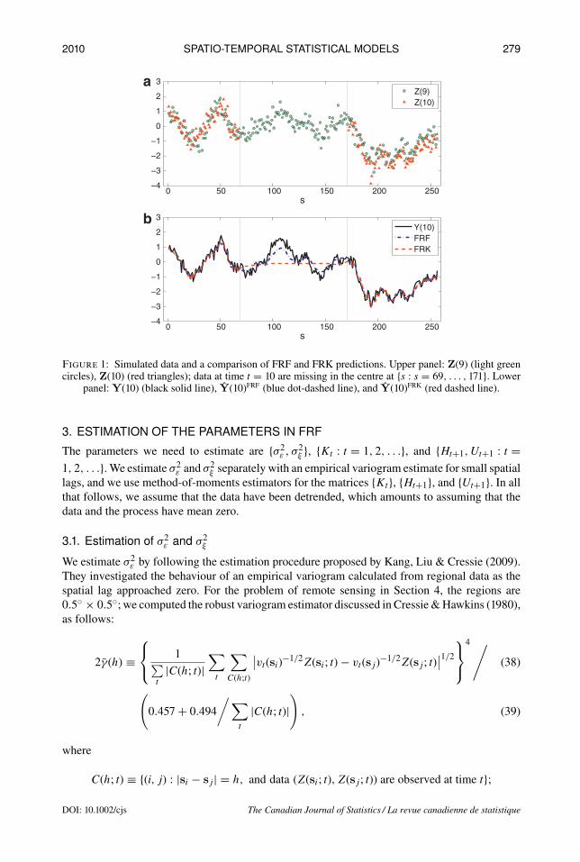
To see the difference between FRF and FRK, we simulated spatio-temporal data {Z(t) : t =1, 2, . . .} on a one-dimensional spatial domain {s : s = 1, . . . , 256}. We used the STRE model(7), (8), and (9), choosing strong temporal dependence. At time point t, we deleted the middle103 observations and computed FRK based on those incomplete current data. We also computedFRF based on the same incomplete current data and complete past data. The result is shown inFigure 1; in the region where data are missing, FRF does a much better job than FRK of trackingthe true process Y (s; t). More detailed discussion of the value of using past data in a dynamicalspatio-temporal model is given by Cressie, Shi & Kang (2010).



0 50 100 150 200 250−4

−3

−2

−1

0

1

2

3

s

Y(10)FRFFRK

0 50 100 150 200 250−4

−3

−2

−1

0

1

2

3a

bs

Z(9)Z(10)

Figure 1: Simulated data and a comparison of FRF and FRK predictions. Upper panel: Z(9) (light greencircles), Z(10) (red triangles); data at time t = 10 are missing in the centre at {s : s = 69, . . . , 171}. Lower

panel: Y(10) (black solid line), Y(10)FRF (blue dot-dashed line), and Y(10)FRK (red dashed line).

3. ESTIMATION OF THE PARAMETERS IN FRF

The parameters we need to estimate are {σ2ε , σ2ξ }, {Kt : t = 1, 2, . . .}, and {Ht+1, Ut+1 : t =1, 2, . . .}. We estimate σ2ε and σ2ξ separately with an empirical variogram estimate for small spatiallags, and we use method-of-moments estimators for the matrices {Kt}, {Ht+1}, and {Ut+1}. In allthat follows, we assume that the data have been detrended, which amounts to assuming that thedata and the process have mean zero.

3.1. Estimation of σ2ε and σ2ξ

We estimate σ2ε by following the estimation procedure proposed by Kang, Liu & Cressie (2009).They investigated the behaviour of an empirical variogram calculated from regional data as thespatial lag approached zero. For the problem of remote sensing in Section 4, the regions are0.5◦ × 0.5◦; we computed the robust variogram estimator discussed in Cressie &Hawkins (1980),as follows:

2γ(h) ≡ 1∑

t

|C(h; t)|∑t

∑C(h;t)

∣∣vt(si)−1/2Z(si; t)− vt(sj)−1/2Z(sj; t)∣∣1/2

4/(38)

(0.457+ 0.494

/∑t

|C(h; t)|)

, (39)

where

C(h; t) ≡ {(i, j) : |si − sj| = h, and data (Z(si; t), Z(sj; t)) are observed at time t};



|C(h; t)| denotes the number of distinct elements of C(h; t), and h is the spatial lag. For example,h is defined in units determined by the pixel size in the application reported in Section 4. If thepixels are square, the spatial lag for two neighbouring pixels is 1, and that between two diagonalpixels in a 2 × 2 block of pixels is

√2.

We plotted the semivariogram against h, for h near the origin. A straight line based on theestimated semivariogram with h close to zero is fitted; for regional data, Kang, Liu & Cressie(2009) show that σ2ε is estimated unbiasedly from the fitted line’s intercept:

σ2ε = γ(0+). (40)

And σ2ξ is estimated from lag-1 squared differences after appropriate adjustment of coefficients:

σ2ξ ≡ 12∑t

|C(1; t)|∑t

∑C(1;t)

{(Z(si; t)− Z(sj; t))2 − σ2ε (vt(si)+ vt(sj))}. (41)

For a detailed definition, estimation, modeling, and a discussion of semivariograms, readers arereferred to Cressie (1993, Section 2.4).

3.2. Estimation of Matrix ParametersWe followed the binning procedure proposed by Cressie & Johannesson (2008) to obtain themethod-of-moments estimators of {Kt}, {Ht+1}, and {Ut+1}.

We chose a set ofM (r < M < n) time-invariant bin centres {uj : j = 1, . . . ,M}, for example,based on25 = 5× 5pixels; in Section 4, the bins are 2.5◦ × 2.5◦. The bins define a neighbourhoodN(uj) of uj , from which we define the 0–1 weights,

wji,t ≡{1 if si,t ∈ N(uj)0 otherwise, (42)

for i = 1, . . . , nt , j = 1, . . . ,M, and t = 1, 2, . . . Denote wj,t ≡ (wj1,t , . . . , wjnt,t)′, and define

the M × M empirical covariance matrices, !M,t ≡ (!M,t(uj,uk)), for t = 1, 2, . . .

!M,t(uj,uk) ≡{∑nt

i=1 wji,tZ(si,t ; t)2/w′j,t1nt , j = k,

Zt(uj)Zt(uk), j �= k,(43)

where Zt(uj) ≡∑nt

i=1 wji,tZ(si,t ; t)/w′j,t1nt , and 1nt is an nt-dimensional vector of 1s. Notice

that there is no mean-correction in (43), since the data are assumed detrended and hence to havemean zero. If the data had trend, we would have to subtract (an estimate of) µ(s; t) in appropriateplaces in (43) and elsewhere.

In a similar way, theM × M empirical lag-1 cross-covariancematrix, !(1)M,t ≡ (!(1)

M,t(uj,uk)),is obtained

!(1)M,t+1(uj,uk) ≡ Zt+1(uj)Zt(uk), (44)

for t = 1, 2, . . .We also define the binned version of St and Vt as St ≡ (S∼t(u∼1), . . . , S∼t(u∼M))′ andVt ≡ diag(v(u1; t), . . . , v(uM ; t))′, whose components are

S∼(u∼j) ≡nt∑i=1

wji,tSt(si,t)/w′j,t1nt , (45)



and

v(uj; t) ≡nt∑i=1

wji,tvt(si,t)/w′j,t1nt , (46)

for j = 1, . . . ,M and t = 1, 2, . . . The same averages were carried out on the nt × nt identitymatrix Int as well, which resulted in an M × M identity matrix IM . Then we can write thetheoretical binned covariance matrix as

!M,t ≡ StKtS′t + σ2ξ IM + σ2ε Vt, (47)

which is an M × M positive-definite matrix.Wewould like to choose positive-definite {Kt} such that !M,t is as “close” to !M,t as possible.

The Frobenius norm is chosen to measure the closeness of the empirical matrix !M,t to thetheoretical matrix !M,t (e.g., Shi & Cressie, 2007; Cressie & Johannesson, 2008):

‖ !M,t − !M,t ‖2≡ tr((!M,t − !M,t)′(!M,t − !M,t)

), (48)

and the estimator of Kt is obtained from minimizing the squared Frobenius norm in (48):

Kt = R−1t Q′

t(!M,t − Dt)Qt(R−1t )′, (49)

where St = QtRt is the Q–R decomposition of St , and Dt ≡ σ2ξ IM + σ2ε Vt .It can be noticed from (49), that !M,t − Dt should be positive-definite to ensure that Kt is

positive-definite. However, the empirical method-of-moments estimates, !M,t , cannot guaranteethat. We propose here a method to adjust !M,t , that not only ensures the positive-definiteness ofKt , but also preserves the total variability of the original estimates !M,t after the adjustment.

To adjust !M,t , we first define

At ≡ D−1/2t (!M,t − Dt)D

−1/2t = D

−1/2t !M,tD

−1/2t − IM. (50)

Notice that Kt is positive-definite if At is. Hence, our aim is to adjust any negative eigenvaluesof At to be positive. Our approach is to “lift” the eigenvalues as follows:

λ∗ ={

λ0 exp{a(λ − λ0)}, λ < λ0

λ, λ ≥ λ0,(51)

where a, λ0 > 0; λ denotes an original eigenvalue of At ; and λ∗ denotes its lifted version. Afterthe lifting algorithm has been applied, the large positive eigenvalues (λ ≥ λ0) will not be changed,the small positive ones will be decreased, and the negative ones will be increased to be positive.In the end, all the lifted eigenvalues will be positive and the original order of eigenvalues will bepreserved.

In (51), we choose λ0 to be the (M − r)/M quantile of all the original eigenvalues, whichleaves the top r eigenvalues unaffected. Further, we choose a ∈ (0,∞) to be that value that leavesthe total variability of the adjusted matrix the same as the original one. That is, let A∗

t denote thematrix corresponding to the lifted eigenvalues and choose a so that,

tr(!∗M,t) = tr(!M,t),



where

!∗M,t ≡ D

1/2t A∗

t D1/2t + Dt,

and from (50),

!M,t = D1/2t AtD

1/2t + Dt.

Finally, the estimator of Kt is obtained from minimizing the Frobenius norm between !∗M,t and

!M,t :

Kt ≡ R−1t Q′

t(!∗M,t − Dt)Qt(R−1

t )′. (52)

The propagator matrix Ht is estimated using a similar binning procedure for the lag-1 cross-covariances. Recall the definition ofLt+1 in (13).Wefit StL

′t S

′t−1 to the empirical binned estimator

of the cross-covariance of Z(t),Z(t − 1), namely, !(1)M,t . From Cressie and Johannesson (2008,

Appendix),

Lt ≡ R−1t−1Q

′t−1(!

(1)M,t)

′Qt(R−1t )′, (53)

where St−1 = Qt−1Rt−1 and St = QtRt are Q–R decompositions, for t = 2, 3, . . .. Bysubstituting Kt−1, Kt , and Lt , given by (52) and (53), into (12) and (13), we obtain

Ht ≡ L′tK

−1t−1 and Ut ≡ Kt − HtLt, (54)

where positive-definiteness of the latter quantity in (54) must be checked.

4. ANALYSIS OF AEROSOL OPTICAL DEPTH (AOD) DATA FROM THE MISRINSTRUMENT

In this section, we illustrate how to apply FRF to a large spatio-temporal data set obtained fromthe MISR instrument, one of NASA’s key instruments measuring and monitoring global aerosoldistributions. The MISR instrument is one of several on NASA’s Terra satellite.

4.1. The MISR Data and its Exploratory Data AnalysisNASA’s Terra satellite was launched onDecember 18, 1999, as part of the Earth Observing System(EOS), and theMISR instruments on board collects global aerosol information, such as AOD, andaerosol shape and size (Diner et al., 1999; Kaufman et al., 2000). Since aerosol forcing contains themajor source of uncertainty in climate forcings in climate models, accurate global aerosol recordsbased on EOS satellites play a vital role in calibrating the climate models, and complete preciseaerosol values are needed. MISR is one key instrument in the EOS for long-term global aerosolmonitoring. The cameras on the instrument cover 233 geographically distinct, but overlappingN–S swaths from the Arctic down to Antarctica, on a repeat cycle of 16 days.

Level-2 aerosol data are collected at a high spatial resolution, 17.6 km × 17.6 km. Thesatellite’s orbit is repeated exactly every 16 days. Level-3 data products are generated from level-2data at a much lower spatial resolution (0.5◦ × 0.5◦), by averaging level-2 observations fallingin the level-3 pixels in a given time period. In this section, we analyze all level-3 data in a studyregion with 128 × 256 =32,768 pixels (0.5◦ × 0.5◦), during the period, July 1, 2001 throughAugust 9, 2001. While the data set is not massive, it involves about 100,000 observations andis large enough to demonstrate our methodology. Cressie, Shi & Kang (2010) considered twotime points of this data set to illustrate the improvement obtained by FRF compared to FRK. Our



0 1 2 30

500

1000

1500

2000

2500

3000

3500

4000

AOD−6 −4 −2 0 20

500

1000

1500

log(AOD)

Figure 2: Left panel: Histogram of the n1=20,970 observations of aerosol optical depth (AOD) at timeunit t = 1. Right panel: Histogram of log(AOD) at time unit t = 1.

purpose in this section is to demonstrate the implementation of FRF over many time points andshow the results on this large spatio-temporal data set.

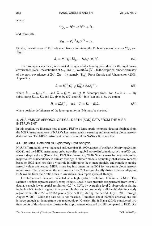
The study region D we chose is the rectangular area between longitudes −125◦ and +3◦ andbetween latitudes −20◦ and +44◦, which covers North and South America, the western part ofthe Sahara desert in Africa, the Iberian Peninsula in Europe, and parts of the Atlantic and PacificOceans, a map of which is given below (in Figure 3). Recall that the data set consists of the MISRlevel-3 AOD data collected between July 1 and August 9, and we chose 8 days as the time unit;that is, time unit 1 corresponds to July 1–8, time unit 2 corresponds to July 9–16, . . ., and timeunit 5 corresponds to August 2–9. The number of data in each of these time units is, respectively,n1 =20,970, n2 =19,398, n3 =20,819, n4=20,167, and n5 =21,759. The choice of 8 days allowedenough spatial coverage to estimate the parameters of the STRE model, but did not compromisethe strength of temporal dependence (Section 4.3).

Shi & Cressie (2007) showed that level-3 AOD data are highly right-skewed, and hence weused the logarithmic transformation as they suggested. Then an individual datum is obtained bytaking a weighted average of daily level-3 log(AOD) values in a given 8-day period with thenumber of level-2 observations Nd(s) in level-3 pixel s on day d as the corresponding weight.Figure 2 shows a histogram of the n1 =20,970 AOD data on the original scale and on the logscale. Henceforth, all analyses are done on log(AOD) data.

After considerable exploratory data analysis, we divided the study region D into three areas:the oceans, the Americas, and the rest (land in the eastern part ofD, namely the Sahara Desert andthe south-western tip of Europe). These are shown in Figure 3. Then, using indicator functions ofthese regions as explanatory variables, we detrended the original data set with a spatial-only linearmodel andordinary least-squares (OL’s) estimation of regression parameters. This created a spatio-temporal data set,Z(1), . . . ,Z(5), uponwhichwe implemented ourmethodology (assumingmeanzero). The trend and the detrended spatio-temporal data set are shown in Figure 3.

We fitted the detrended spatio-temporal log(AOD) data set with the STRE model given by(21) and µ(s; t) equal to 0. We chose time-invariant S(·) from multi-resolution W-wavelet basisfunctions using the strategy given by Shi & Cressie (2007). All the 32 W-wavelets from thefirst scale and the 62 W-wavelets from the second scale with “large” absolute coefficients were



Figure 3: Data are log(AOD). The (OLS estimated) trend is shown in the upper-left panel. The otherpanels show the detrended data, Z(1), . . . ,Z(5), for which the number of data are n1=20,970, n2 =19,398,

n3=20,819, n4=20,167, and n5=21,759, respectively.

chosen, which resulted in r = 32 + 62 = 94, for all t. Recall that the level-3 data were generatedby averaging (over days) the level-2 MISR data. Hence, we assume in (1) that vt(s) = 1/Nt(s),where {Nt(s) : s ∈ D} is the number of level-2 observations obtained during time unit t in therespective pixels of D.

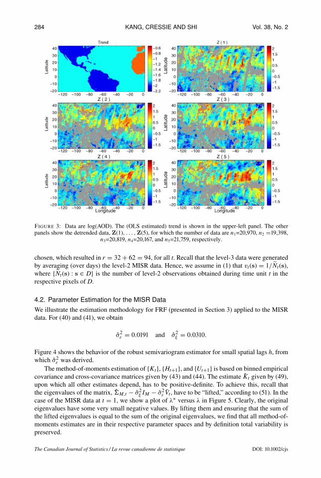
4.2. Parameter Estimation for the MISR DataWe illustrate the estimation methodology for FRF (presented in Section 3) applied to the MISRdata. For (40) and (41), we obtain

σ2ε = 0.0191 and σ2ξ = 0.0310.

Figure 4 shows the behavior of the robust semivariogram estimator for small spatial lags h, fromwhich σ2ε was derived.

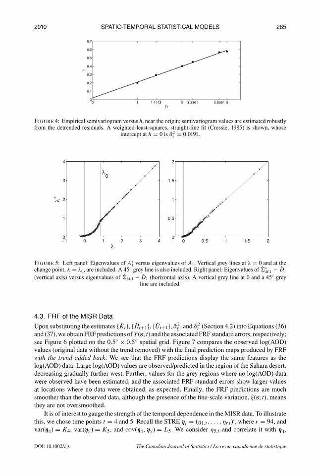
The method-of-moments estimation of {Kt}, {Ht+1}, and {Ut+1} is based on binned empiricalcovariance and cross-covariance matrices given by (43) and (44). The estimate Kt given by (49),upon which all other estimates depend, has to be positive-definite. To achieve this, recall thatthe eigenvalues of the matrix, !M,t − σ2ξ IM − σ2ε Vt , have to be “lifted,” according to (51). In thecase of the MISR data at t = 1, we show a plot of λ∗ versus λ in Figure 5. Clearly, the originaleigenvalues have some very small negative values. By lifting them and ensuring that the sum ofthe lifted eigenvalues is equal to the sum of the original eigenvalues, we find that all method-of-moments estimates are in their respective parameter spaces and by definition total variability ispreserved.



Figure 4: Empirical semivariogram versus h, near the origin; semivariogram values are estimated robustlyfrom the detrended residuals. A weighted-least-squares, straight-line fit (Cressie, 1985) is shown, whose

intercept at h = 0 is σ2ε = 0.0191.

−1 0 1 2 3 40

1

2

3

4

λ

λ∗

λ0

0 0.5 1 1.5 20

0.5

1

1.5

2

Figure 5: Left panel: Eigenvalues of A∗1 versus eigenvalues of A1. Vertical grey lines at λ = 0 and at the

change point, λ = λ0, are included. A 45◦ grey line is also included. Right panel: Eigenvalues of !∗M,1 − D1

(vertical axis) versus eigenvalues of !M,1 − D1 (horizontal axis). A vertical grey line at 0 and a 45◦ greyline are included.

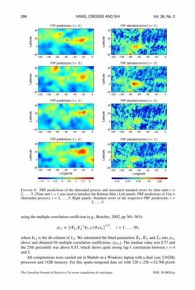
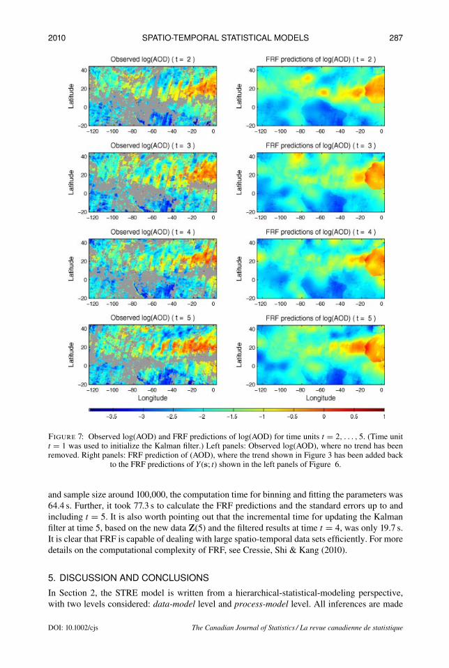
4.3. FRF of the MISR DataUpon substituting the estimates {Kt}, {Ht+1}, {Ut+1}, σ2ξ , and σ2ε (Section 4.2) into Equations (36)and (37),we obtain FRFpredictions ofY (s; t) and the associated FRF standard errors, respectively;see Figure 6 plotted on the 0.5◦ × 0.5◦ spatial grid. Figure 7 compares the observed log(AOD)values (original data without the trend removed) with the final prediction maps produced by FRFwith the trend added back. We see that the FRF predictions display the same features as thelog(AOD) data: Large log(AOD) values are observed/predicted in the region of the Sahara desert,decreasing gradually further west. Further, values for the grey regions where no log(AOD) datawere observed have been estimated, and the associated FRF standard errors show larger valuesat locations where no data were obtained, as expected. Finally, the FRF predictions are muchsmoother than the observed data, although the presence of the fine-scale variation, ξ(s; t), meansthey are not oversmoothed.

It is of interest to gauge the strength of the temporal dependence in theMISR data. To illustratethis, we chose time points t = 4 and 5. Recall the STRE ηt = (η1,t , . . . , ηr,t)′, where r = 94, andvar(η4) = K4, var(η5) = K5, and cov(η4, η5) = L5. We consider η5,i and correlate it with η4,



Figure 6: FRF predictions of the detrended process and associated standard errors for time units t =2, . . . , 5. (Time unit t = 1 was used to initialize the Kalman filter.) Left panels: FRF predictions of Y (s; t)(detrended process); t = 2, . . . , 5. Right panels: Standard errors of the respective FRF predictions; t =

2, . . . , 5.

using the multiple correlation coefficient (e.g., Rencher, 2002, pp 361–363):

ρ5,i ≡ {(�′5,iK

−14 �5,i)/(K5)ii

}1/2, i = 1, . . . , 94,

where �5,i is the ith column of L5. We substituted the fitted parameters K4, K5, and L5 into ρ5,iabove and obtained 94 multiple correlation coefficients, {ρ5,i}. The median value was 0.77 andthe 25th percentile was above 0.53, which shows quite strong lag-1 correlation between t = 4and 5.

All computations were carried out in Matlab on a Windows laptop with a dual core 2.0GHzprocessor and 3GB memory. For this spatio-temporal data set with 128 × 256 =32,768 pixels



Figure 7: Observed log(AOD) and FRF predictions of log(AOD) for time units t = 2, . . . , 5. (Time unitt = 1 was used to initialize the Kalman filter.) Left panels: Observed log(AOD), where no trend has beenremoved. Right panels: FRF prediction of (AOD), where the trend shown in Figure 3 has been added back

to the FRF predictions of Y (s; t) shown in the left panels of Figure 6.

and sample size around 100,000, the computation time for binning and fitting the parameters was64.4 s. Further, it took 77.3 s to calculate the FRF predictions and the standard errors up to andincluding t = 5. It is also worth pointing out that the incremental time for updating the Kalmanfilter at time 5, based on the new data Z(5) and the filtered results at time t = 4, was only 19.7 s.It is clear that FRF is capable of dealing with large spatio-temporal data sets efficiently. For moredetails on the computational complexity of FRF, see Cressie, Shi & Kang (2010).

5. DISCUSSION AND CONCLUSIONS

In Section 2, the STRE model is written from a hierarchical-statistical-modeling perspective,with two levels considered: data-model level and process-model level. All inferences are made



according to an empirical-Bayesian framework. That is, estimates of parameters are substitutedinto the FRF equations (without accounting for their sampling variances). By adding a third level,that is, a parameter-model level (i.e., prior model), a fully Bayesian framework can be derived inprinciple. Choice of priors and speed of convergence of anyMarkov chainMonte Carlo algorithminvolved in fullyBayesian inference are important issues thatwill be addressed elsewhere.Anotheradvantage of a fully Bayesian approach is that it has more flexibility in dealing with non-Gaussiandata and a nonlinear process model.

The covariance structure of the fine-scale variation referred to above is modeled as a multipleof the identity matrix. Generalizations to other structures include a diagonal matrix or a finer-scale variation modeled by spatial basis functions at finer resolutions, namely SξKξS

′ξ . Then a

similar estimation procedure would proceed as demonstrated in Section 3. Associated with thespecification of the covariance structure to describe the spatial variation is the choice of numberof basis functions applied in the STRE model (i.e., the choice of r). This and the type of basisfunctions chosen is a problem that will be addressed elsewhere.

FRF is an optimal spatio-temporal predictor that is able to incorporate both current and pastinformation efficiently for processing large spatio-temporal data sets. Through the applicationof our method to a data set from NASA’s MISR instrument on the Terra satellite, we havedemonstrated in detail how the parameters in the model are estimated and how FRF is ableto combine current and past data optimally, to provide a complete map of estimated (log)aerosol optical depth values. Importantly, the FRF predictions are accompanied by their respectiveprediction standard errors.

ACKNOWLEDGEMENTSThe authors would like to thank an anonymous referee and the editor of the special issue, Prof.Brajendra Sutradhar, for their helpful comments. This research was supported by the NationalScience Foundation under award DMS-0707009 (Kang), the Office of Naval Research underGrant N00014-08-1-0464 (Cressie), the National Aeronautics and Space Administration (NASA)under grant NNX08AJ92G issued through the ROSES Carbon Cycle Science Program and GrantNNH08ZDA001N issued through the Advanced Information Systems Technology ROSES 2008Solicitation (Cressie), and NASA grant NNG06GD31G (Shi). MISR data were obtained bycourtesy of the NASA Langley Research Atmospheric Science Data Center.

BIBLIOGRAPHYB. D. O. Anderson (1984). “Adaptive Control,” Pergamon Press, Oxford.S. Banerjee, A. E. Gelfand, A. O. Finley & H. Sang (2008). Gaussian predictive process models for large

spatial data sets. Journal of the Royal Statistical Society, Series B, 70, 825–848.R. A. Bilonick (1983). Risk qualified maps of hydrogen ion concentration for the New York state area for

1966–1978. Atmospheric Environment, 17, 2513–2524.N. Cressie (1985). Fitting variogram models by weighted least squares. Journal of the International

Association for Mathematical Geology, 17, 563–586.N. Cressie (1993). “Statistics for Spatial Data,” revised edition, Wiley, New York.N. Cressie & D. M. Hawkins (1980). Robust estimation of the variogram, I. Journal of the International

Association of Mathematical Geology, 12, 115–125.N. Cressie & G. Johannesson (2006). Spatial prediction of massive datasets. Proceedings of the Australian

Academy of Science Elizabeth and Frederick White Conference. Australian Academy of Science,Canberra, pp 1–11.

N. Cressie & G. Johannesson (2008). Fixed rank kriging for very large spatial data sets. Journal of the RoyalStatistical Society, Series B, 70, 209–226.



N. Cressie & E. L. Kang (2010). “High-resolution digital soil mapping: Kriging for very large datasets,”in “Proximal Soil Sensing,” R. Viscarra-Rossel, A. B. McBratney and B. Minasny, editors. Elsevier,Amsterdam (in press).

N.Cressie, T. Shi&E.L.Kang (2010). Fixed rankfiltering for spatio-temporal data. Journal ofComputationaland Graphical Statistics, forthcoming.

D. J. Diner, G. P. Asner, R. Davies, Y. Knyazikhin, J. Muller, A. W. Nolin, B. Pinty, C. B. Schaaf & J.Stroeve (1999). New directions in earth observing scientific applications of multiangle remote sensing.Bulletin of the American Meteorological Society, 80, 2209–2228.

H. V. Henderson & S. R. Searle (1981). On deriving the inverse of a sum of matrices. SIAM Review, 23,53–60.

R. E. Kalman (1960). A new approach to linear filtering and prediction problems. Journal of BasicEngineering, Series D, 82, 35–45.

E. E. Kammann & M. P. Wand (2003). Geoadditive models. Applied Statistics, 52, 1–18.E. L. Kang (2009). Reduced-dimension hierarchical statistical models for spatial and spatio-temporal data.

Ph.D. Dissertation, Department of Statistics, The Ohio State University, Columbus.E. L. Kang, D. Liu&N. Cressie (2009). Statistical analysis of small-area data based on independence, spatial,

non-hierarchical, and hierarchical models. Computational Statistics and Data Analysis, 53, 3016–3032.Y. J. Kaufman, B. N. Holben, D. Tanre, I. Slutsker & A. Smirnov (2000). Will aerosol measurements

from Terra and Aqua polar orbiting satellites represent the daily aerosol abundance and properties?Geophysical Research Letters, 27, 3861–3864.

D. Nychka, B. Bailey, S. Ellner, P. Haaland&M.O’Connell (1996).FUNFITS: Data Analysis and StatisticalTools for Estimating Functions. North Carolina Institute of Statistics Mimeo Series No. 2289

D. Nychka, C. K. Wikle & J. A. Royle (2002). Multiresolution models for nonstationary spatial covariancefunctions. Statistical Modeling, 2, 315–331.

A. C. Rencher (2002). “Methods of Multivariate Analysis,” 2nd ed., Wiley, New York.S. Rouhani &H.Wackernagel (1990).Multivariate geostatistical approach to space-time data analysis.Water

Resources Research, 26, 585–591.T. Shi & N. Cressie (2007). Global statistical analysis of MISR aerosol data: A massive data product from

NASA’s Terra satellite. Environmetrics, 18, 665–680.R. H. Shumway & D. S. Stoffer (2006). “Time Series Analysis and Its Applications, With R Examples,” 2nd

ed., Springer, New York.G. Sneddon & B. C. Sutradhar (2004). On semiparametric familial-longitudinal models. Statistics &

Probability Letters, 69, 369–379.C. K.Wikle&N. Cressie (1999). A dimension-reduced approach to space-timeKalman filtering.Biometrika,

86, 815–829.

Received 7 May 2009Accepted 30 November 2009


using temporal variability to improve spatial mapping with application to satellite data

Documents