using the transferable belief model and a qualitative possibility theory approach on an illustrative...

Using the Transferable Belief Modeland a Qualitative Possibility TheoryApproach on an Illustrative Example:The Assessment of the Value of aCandidate*

Didier Dubois,1 Michel Grabisch,2 Henri Prade,1 Philippe Smets,3,†1Institut de Recherche en Informatique de Toulouse (IRIT)–CNRS,Université Paul Sabatier, 118 route de Narbonne, 31062Toulouse Cedex 4, France2Thomson-CSF, Corporate Research Laboratory, Domaine de Corbeville,91404 Orsay, France3IRIDIA, Université Libre de Bruxelles, 50 av. Roosevelt, CP 194-6,1050 Bruxelles, Belgium

The problem of assessing the value of a candidate is viewed here as a multiple combinationproblem. On the one hand, a candidate can be evaluated according to different criteria,and on the other hand, several experts are supposed to assess the value of candidatesaccording to each criterion. Criteria are not equally important, experts are not equallycompetent or reliable. Moreover, levels of satisfaction of criteria, or levels of confidenceare only assumed to take their values in linearly ordered scales, whose nature is ratherqualitative. The problem is discussed within two frameworks, the transferable belief model(TBM) and the qualitative possibility theory (QPT). They respectively offer a quantitativeand a qualitative setting for handling the problem, thus providing a way to emphasizewhat are the underlying assumptions in each approach. © 2001 John Wiley & Sons, Inc.

*This paper is a revised, unified and extended version of two conference papers[Refs. 7 and 8], the second being only devoted to the possibility approach.

†Author to whom correspondence should be addressed; e-mail: [email protected] grant sponsor: European working group FUSION (Esprit Project 20001:

Fusion of Uncertain Data from Sensors, Information Systems and Expert Opinions).

INTERNATIONAL JOURNAL OF INTELLIGENT SYSTEMS, VOL. 16, 1245–1272 (2001)© 2001 John Wiley & Sons, Inc.

1246 DUBOIS ET AL.

1. INTRODUCTION

1.1. Preamble

The purpose of this paper is essentially to show how to apply two uncertaintymodeling frameworks, the transferable belief model (TBM) and the qualitativepossibility theory (QPT) approaches, to a complex problem that combines, vol-untarily, many difficulties. The problem concerns the assessment of the value ofa candidate evaluated by several experts using several criteria. Thus it exhibitsboth a multiple-criteria decision making and a data fusion facet. Moreover it isassumed that for each criteria, there exists a unique value, usually pervaded withuncertainty, which represents the true value of the candidate w.r.t. the criterion.The example is only illustrative, and we do not claim the techniques exemplifiedhere are the best methods to solve the problem. Other approaches more dedi-cated to multiple criteria or group decision could be defended as well. In fact, theexample is envisaged mainly as a multiple-sensor problem in the TBM approach,while the QPT-based method distinguishes the fusion of expert opinions fromthe multiple criteria aggregation. The paper shows how the two representationframeworks can be used in practice, rather than discussing the appropriatenessof the solutions proposed w.r.t. the value assessment problem.

1.2. Introducing the Example

The problem of assessing the value of a candidate (it may be a person, anobject, or any abstract entity for instance) is often encountered in practice. It isusually a preliminary step before making a choice. Such a problem can be han-dled in different manners depending on what kind of information the evaluationis based. One may have expert generic rules which aim at classifying candidatesin different categories (e.g., “excellent,” “good,” � � � , “very bad”). One may havea base of examples made of previous evaluations from which a similarity-basedevaluation of the new candidate can be performed. This corresponds to two pop-ular approaches in Artificial Intelligence (namely, expert systems and case-basedreasoning), that one might also like to combine.

In the following, the value assessment problem is posed rather in terms ofmultiple-criteria evaluation, whose value for a given candidate can be more orless precisely assessed with some level of confidence by various experts (whoseopinions are also to be fused). This problem is sometimes referred to as a subjec-tive evaluation process.4 For a discussion of the relation between the rule-, case-and criteria-based approaches, the reader is referred to Refs. 11 and 13. Notethat the problem considered in the following is not simply to rank-order candi-dates on the basis of a set of criteria; pairwise comparisons could then lead toa simple outranking solution. The problem here is to design a procedure wheremultiple expert assessments are faithfully represented and fused. As we shall seedifferent families of solutions are possible according to the way the criteria areinteracting.

An important issue in such a problem is that the assessment of the valuesof the criteria for a candidate by an expert and their relevance for the selection

TRANSFERABLE BELIEF AND QUALITATIVE POSSIBILITY THEORY 1247

itself are often pervaded with uncertainty and imprecision. Numerical or quali-tative modeling of the data can be considered. In this paper, we show how theTBM,24 and QPT can be applied to the value assessment problem, thus illustrat-ing the two types of approaches, and showing how the methods can be applied.Moreover their underlying assumptions are laid bare.

The paper is organized into four main parts. The problem is first preciselystated and the questions that it raises are pointed out. Then the two proposedapproaches are presented and illustrated on the same example. Finally, a com-parative discussion of the two approaches is given.

2. THE MULTIPLE-EXPERT MULTIPLE-CRITERIAASSESSMENT PROBLEM

The value of a candidate for a given position has to be assessed by a decisionmaker (DM). For this evaluation, m criteria are used. For each criterion, thevalue of the candidate is assessed (maybe imprecisely) by n experts (or sources).Criteria can be rank-ordered according to their importance for the position. Theirrelation to the global “goodness” score of the candidate for the position mayalso be available. Each expert provides a precise or imprecise evaluation for eachcriterion and a level of confidence is attached to each evaluation by the expertwho is responsible for it. The general reliability of each expert is also qualitativelyassessed by DM.

Some general comments about the problem which so far is informally stated,have to be made. With a set of candidates, one may want to (i) choose thebest one(s); (ii) rank all candidates from best to worst; (iii) give a partial orderbetween them, with possibly some incomparabilities; (iv) cluster the candidatesin several groups (e.g., good ones, bad ones, those with a weak point w.r.t. onecriterion, etc.). In fact, many methods in decision analysis proceed by a pairwisecomparison of candidates which supposes all of them are known from the begin-ning. In this paper, we look for the global evaluation of a candidate which maybe unique. If the problem were to rank-order candidates only, a lexicographicapproach (based on the comparison of vectors made of scores of each candi-date w.r.t. all criteria ordered according to their importance) might be sufficient.However, such an approach assumes that a complete order exists between scores(which is not in agreement with the fact that the scores may be imprecise andpervaded with uncertainty).

The overall assumption of the model underlying our example is that thereexist true scores for each individual criterion and for a global goodness, allattached to the candidate, the last being a function of the first ones. The problemis that these true values are unknown to the DM and must be estimated fromthe expert opinions.

This approach is thus an estimation problem where the experts are consid-ered as measurement tools or sensors that determine some kind of “objective”parameters. Other approaches based on classical multiple-criteria decision mak-ing could of course have been defended. As already said, comparing the merits

1248 DUBOIS ET AL.

of other such methods is not the purpose of this paper. We focus on how to applytwo particular methods, not on deciding which is good or bad.

2.1. Notations

Now we introduce some notation. The candidate is denoted K, when nec-essary. Criteria are numbered by i: i = 1� � � � �m. The true (unknown) valueof the level of satisfaction of criterion i for the candidate K is denoted ciK,with ciK ∈ Ls, where Ls is the ordinal scale of levels of satisfaction, e.g., Ls =�1� 2� 3� 4� 5 with 1=very bad, � � � , 5=very good. An element of Ls is denotedby s.

Experts are numbered by j: j = 1� � � � � n. The function �ji is a mapping

from Ls to L� . In the example we shall use L� = �� a� b� � which is anordinal scale, where � corresponds to impossibility, and � to total possibility.The true (unknown) global score of K is denoted cK ∈ Ls. The confidenceof the decision maker in expert j when judging criterion i is denoted �ij , andthese levels are defined on an ordinal scale L� which can be related to L� as weshall see. The confidence of the decision maker in expert j ’s opinions is denoted�j� j = 1� � � � � n, and the �j ’s are defined on an ordinal scale L�. For instance,L� = �� u� v� � with � = not confident at all, u = not very confident, � � � , � =very confident. The levels of importance of criteria are denoted �i� i = 1� � � � �m,and the �i also belong to an ordinal scale L�. For instance L� = �� e� f � g� � with � = not important at all, e = not very important, � � � , � = veryimportant.

2.2. Data for the Example

For illustrative purpose we use the following example with m = 6 criteriaand n = 4 experts. Imagine that in some company, a new collaborator K hasto be hired for the marketing department. Six criteria are used for assessing hisqualifications: analysis capacities (Ana), learning capacities (Lear), past experi-ence (Exp), communication skills (Com), decision-making capacities (Dec) andcreativity (Crea). The four experts are the directors of Marketing (Mkt), Finan-cial (Fin), Production (Prod), and Human Resources (HR) departments. Thedata are summarized in Table I. Blanks correspond to missing values, i.e., thedirector did not provide an evaluation for the considered criteria. In fact all miss-ing values correspond here to the criteria i for which the expert j is consideredby DM as not competent (�ij = �). They may be assimilated to a �0� 5� assess-ment as we equate “no opinion” to “opinion not provided,” a natural assumptionhere.

On the one hand this example is intentionally complex as we want to illus-trate the power and flexibility of the two approaches. On the other hand, theway the criteria should be aggregated is unspecified. In real life, some of thesubtleties introduced here will be irrelevant, simplifying the computation of thesolution.


Table I. Assessment by each director on each criteria of candidate Kusing Ls = 1� 2� 3� 4� 5, and confidence of directors w.r.t. each criteria.

Mkt D Fin D Prod D HR D

(a) Collected data (Cij)Ana 4 2Lear [2,3] [1,5] 4 [2,4]Exp 4Com 4 4Dec [1,5] [1,5] [1,2] 3Crea 5 1

(b) Confidence given by DM (�ij) �i

Ana � � � � gLear b a b � eExp � � � � eCom � � � � �Dec a a a a gCrea � � � � �

�j � u u v

3. THE TBM APPROACH

To represent belief functions, we use the next notational convention: bel�Y[PEV] 0 ∈ A denotes the strength of the weighted opinion (called belief) heldby the agent Y about the fact that the actual world 0 belongs to A, a subset ofthe frame of discernment �, given the piece of evidence PEV. Thanks to the factwe use the same indexing for the basic belief assignments, the belief functionsand the plausibility functions induced by each other, we can just use the notationsm�Y �PEV �, bel

�Y �PEV� and pl�Y �PEV�, the indexing indicating their mutual links.

Many beliefs are used in this example. They are analogous to subjectiveprobabilities, except that they do not satisfy the additivity rule of probabilitytheory. Their operational meaning and their assessment are obtained by methodssimilar to those used by the Bayesians.23

3.1. DM’s Beliefs on the Real Value of Each Criteria

In this section, we consider only candidate K and all beliefs are held by oneDM, so we can avoid mentioning them. Let ci be the actual (but unknown) valueof the level of satisfaction of criterion i. Let Cij denote the data collected fromdirector j on criteria i (for K), Cij being the intervals given in Table I. Missingdata are equated to the whole interval [1, 5].

Let %Cij = a � ci = x be the degree of (quantitative) possibility‡ thatDirector j states Cij = �a� a� with a ∈ �1� � � � � 5 given ci = x with x ∈ �1� � � � � 5 .

‡Here we use quantitative possibilities ranging in [0,1], whereas in the QPT approach,only qualitative possibilities are considered. The link between plausibilities and possibili-ties (pl = %) requires that possibilities be somehow quantified.

1250 DUBOIS ET AL.

It represents the link between what the director will say and the actual valueci. For simplicity’s sake, we use the same possibility function for every criteriaand every director. For each criteria, we assume that the possibility is 1 whena = x� 0'5 when �a− x� = 1, and 0 otherwise. More complex possibility functionscould be used, the proposed one being only “reasonable.” It reflects the idea thatit is (fully) possible that the director states the actual value, “quite possible” thathe states a value at one level deviation from the actual value, and impossible attwo level deviations (director can be wrong, but the error will be small).

A few classical relations are needed. We have:

if %A = p then plA = p� (1)

%X � Y%Y = %Y � X%X� (2)

%X = maxx∈X

%x (3)

We also assume a total a priori ignorance on Cij and ci, i.e.,

%Cij = 1 ∀Cij and %ci = 1 ∀ci' (4)

Using these relations, the degree of plausibility held by DM (before consid-ering DM’s opinions about Director j ’s opinions) that the actual value of ci is inA ⊆ Lsi where Lsi is the domain of ci (equal to Ls in this example), given whatthe Director j states about criteria i, is given by:

plLsi �Cij �ci ∈ A = %ci ∈ A � Cij by 1

= maxx∈A

%ci = x � Cij by 3

= maxx∈A

%Cij � ci = x by 2 and 4

= maxx∈A�a∈Cij

%�a� a� � ci = x by 3

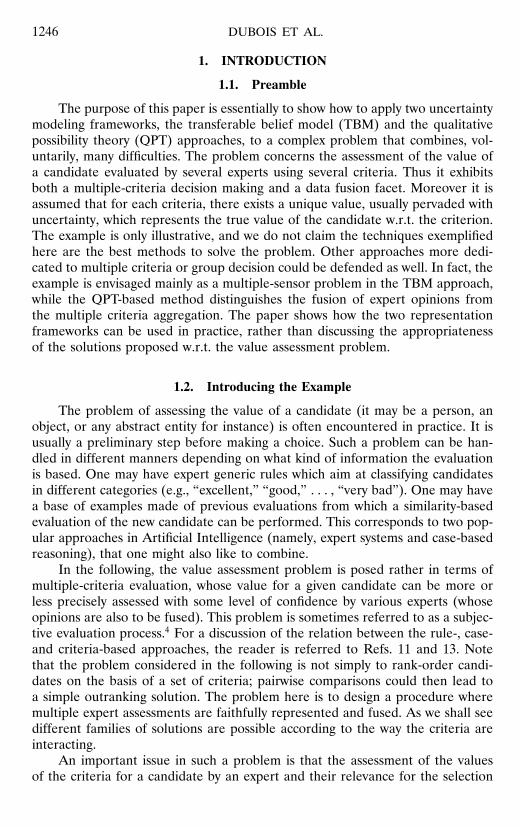
Table II presents the focal elements of the basic belief assignments derivedfrom each informative Cij .

The DM has some weighted opinions about the reliability of the assessmentprovided by Director j on criteria i, represented by the coefficients �ij (numeri-cally rescaled into gij = 0� 1� 2� 3 for �ij = �� a� b� �, respectively). DM also hassome prior opinions about the importance that he should give to Director j ’sopinions when it comes to evaluating a candidate for a position like the openone, opinions that were coded by �j (numerically rescaled into sj = 1� 2� 3 for�j = r� s� �, respectively). All these opinions are transformed into discountingfactors that express how much belief DM should give to the beliefs induced bythe data produced by Director j on criteria i. The discounting factors dij aredecreasing when the � and � values increase.

Discounting factors are meta-beliefs, i.e., beliefs over beliefs. They wereintroduced in Ref. 20, and their formal nature explained in Ref. 21. Their real


Table II. List of the individual informative Cij and the non-zero basicbelief masses of mLsi �Cij � induced on the space Ls = �1� 2� 3� 4� 5 'a

Director Criteria Cij Focus :m Focus : m

Mkt Lear [2,3] 1234 , 0'5 23 , 0'5Mkt Exp 4 345 , 0'5 4 , 0'5Mkt Com 4 345 , 0'5 4 , 0'5Mkt Crea 5 45 , 0'5 5 , 0'5Fin D Ana 4 345 , 0'5 4 , 0'5Prod D Ana 2 123 , 0'5 2 , 0'5Prod D Lea 4 345 , 0'5 4 , 0'5Prod D Dec [1,2] 123 , 0'5 12 , 0'5HR D Lear [2,4] 12345 , 0'5 234 , 0'5HR D Com 4 345 , 0'5 4 , 0'5HR D Dec 3 234 , 0'5 3 , 0'5HR D Crea 1 12 , 0'5 1 , 0'5

aThe basic belief masses are presented as a pair where the first term isthe list of the elements of Ls that belong to the focal element and the secondterm is the value of the mass itself.

assessment is done as for any belief. For the purpose of the example, we use thevalues obtained from the relation:

dij = 1 − 0'95 × gij/3× 0'75 + 0'25 × sj − 1/2'

So dij = 1 in the worst case where gij = 0� and 0.05 in the best case wheregij = 3 and sj = 3. The dij used here are of course arbitrary. In real application,their evaluation would be part of the whole assessment procedure.

Given the coefficients dij , DM discounts mLsi �Cij � obtained from plLsi �Cij �derived just above into mLsi �Eij � where:

mLsi �Eij �A = 1 − dij×mLsi �Cij �A if A = �1� 5��

mLsi �Eij ��1� 5� = 1 − dij×mLsi �Cij ��1� 5�+ dij

The basic belief assignmentmLsi �Eij �, presented in Table III represents DM’sbeliefs about the actual value of ci given the piece of evidence Eij that is equalto what Director j has stated and DM’s opinions about j ’s opinions (the �’s andthe �’s).

Then DM combines the Directors’ opinions over Criteria i by applying the(unnormalized) Dempster’s rule of combination to the discounted basic beliefassignments. The resulting basic belief assignment mLsi �&jEij �, presented inTable IV, represents DM’s beliefs about the actual value of ci.

mLsi �&jEij � =⊕j

mLsi �Eij �

1252 DUBOIS ET AL.

Table III. List of discounting factors dij for the individual informative Cij and the non-zero basic belief masses of mLsi �Eij � induced on the space Ls = �1� 2� 3� 4� 5 'a

Director Criteria dij Focus :m Focus :m Focus :m

Mkt Lear 0.367 1234 , 0'317 23 , 0'317 12345 , 0'367Mkt Exp 0.050 345 , 0'475 4 , 0'475 12345 , 0'050Mkt Com 0.050 345 , 0'475 4 , 0'475 12345 , 0'050Mkt Crea 0.050 45 , 0'475 5 , 0'475 12345 , 0'050Fin D Ana 0.287 345 , 0'356 4 , 0'356 12345 , 0'288Prod D Ana 0.287 123 , 0'356 2 , 0'356 12345 , 0'288Prod D Lea 0.525 345 , 0'238 4 , 0'238 12345 , 0'525Prod D Dec 0.762 123 , 0'119 12 , 0'119 12345 , 0'763HR D Lear 0.169 234 , 0'416 12345 , 0'584HR D Com 0.169 345 , 0'416 4 , 0'416 12345 , 0'169HR D Dec 0.723 234 , 0'139 3 , 0'139 12345 , 0'723HR D Crea 0.169 12 , 0'416 1 , 0'416 12345 , 0'169

aThe basic belief masses are presented as a pair where the first term is the list of the elementsof Ls that belong to the focal element and the second term is the value of the mass itself.

3.2. DM’s Beliefs on the Real Value of the Goodness Score

The real problem for DM is not to assess the actual value of each criterion,but to assess if candidate K is “good” for the position to be filled. So we introducea “goodness score,” that will vary from 1 to 5, 1 for “very bad,” 5 for “very good.”The relation between the goodness score (G. Sc) and the value xi of criterion idepends only on �i, the level of importance of criterion i. The values of fixi aretabulated in Table V. For example, when �i = g, DM accepts as “good” (score 5)a candidate for whom the criterion value xi is 4 or 5. In practice, these valuesmust be assessed through an analysis of the compensatory relation between thescores. For example, it is as “good” to have a score 3 for a criterion which hasimportance � than to have a score 3 when the importance is g and to have ascore 2 when the importance is e.

Table IV. For each criteria, list of non-zero basic belief masses of mLsi �&jEij � obtainedby combining the discounted basic belief assignments obtained from each director.a

Ana Lear Exp Com Dec CreaFocus, m Focus :m Focus :m Focus :m Focus :m Focus :m

� , 0'381 � , 0'075 4 , 0'475 4 , 0'475 � , 0'016 � , 0'7902 , 0'102 3 , 0'075 345 , 0'475 345 , 0'475 2 , 0'016 1 , 0'0213 , 0'127 23 , 0'166 12345 , 0'050 12345 , 0'050 12 , 0'086 12 , 0'021

123 , 0'102 4 , 0'162 3 , 0'122 5 , 0'0804 , 0'102 34 , 0'111 23 , 0'016 45 , 0'080

345 , 0'102 234 , 0'149 123 , 0'086 12345 , 0'00812345 , 0'083 1234 , 0'097 234 , 0'106

345 , 0'051 12345 , 0'55112345 , 0'112

aThe basic belief masses are presented as a pair where the first term is the list of the elementsof Ls that belongs to the focal element and the second term is the value of the mass itself.


Table V. Values of the goodness score fixgiven the score x of criteria i (from 1 to 5) andits level of importance �i.

�i 1 2 3 4 5

e 1 3 4 5 5f 1 2 4 5 5g 1 2 3 5 5� 1 2 3 4 5

Let fix be the value of the G. Sc when the score for criteria i is x andlet fiA = �fix , x ∈ A . Then the belief over the value of the criterion i istransformed into a belief mG�Ci� over the G. Sc by

mG�Ci�B =∑

A,fiA=BmLsi �&jEij �A for B ⊆ �1� 2� 3� 4� 5�

This just means that the basic belief mass mLsi �&jEij �A given to A istransferred to the image of A under the transformation fi that holds betweenthe criterion value and the G. Sc.

The basic belief assignment mG�Ci� derived from the basic belief assignmentmG�Ci� represents DM’s beliefs about the value of the G. Sc of the candidategiven what DM collected about the criteria i. These basic belief assignments arethen combined on i by Dempster’s rule of combination.

mG�&iCi� =⊕i

mG�Ci�

The resulting basic belief assignment mG�&iCi� represents DM’s beliefs overthe value of the goodness score of candidate K given the collected informationand all DM’s a priori about the various criteria importance and the directorscompetence.

Table VI. For each criteria, list of non-zero basic belief masses of mG�Ci� obtained onthe G. Sc using the appropriate fi functions.a

Ana Lear Exp Com Dec CreaFocus :m Focus :m Focus :m Focus :m Focus :m Focus :m

� , 0'381 � , 0'075 4 , 0'475 4 , 0'475 � , 0'016 � , 0'7902 , 0'102 4 , 0'075 345 , 0'475 345 , 0'475 2 , 0'016 1 , 0'0213 , 0'127 34 , 0'166 12345 , 0'050 12345 , 0'050 12 , 0'086 12 , 0'021

123 , 0'102 5 , 0'162 3 , 0'122 5 , 0'0804 , 0'102 45 , 0'162 23 , 0'016 45 , 0'080

345 , 0'102 345 , 0'149 123 , 0'086 12345 , 0'00812345 , 0'083 12345 , 0'210 234 , 0'106

12345 , 0'551aThe basic belief masses are presented as a pair where the first term is the list of the elements

of Ls that belong to the focal element and the second term is the value of the mass itself.

1254 DUBOIS ET AL.

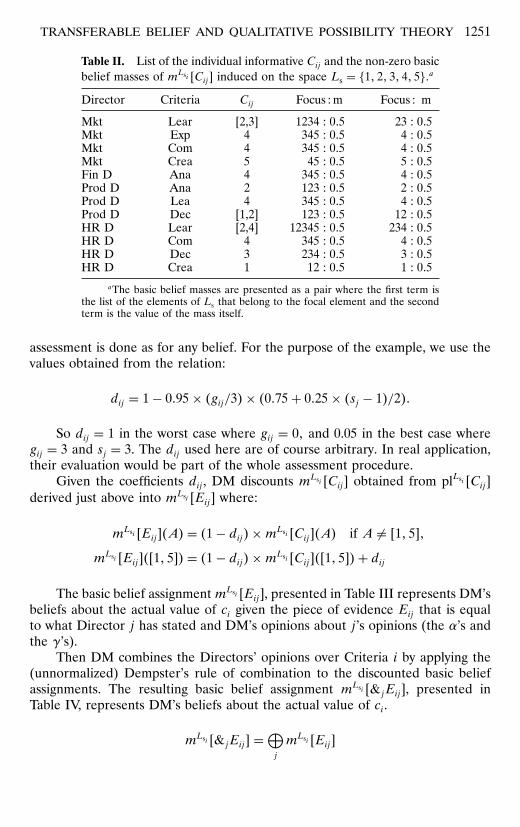
Table VII. Focal sets of mG�&iCi� and their masses on the G.Sc, and non-zero values of BetPG on the singletons of G.

Focal sets � 4 5 {4,5}

mG�&iCi� 0'9858 0'00276 0'00988 0'001537mG�&iCi� Normalized 0 0'34 0'58 0'08BetPG 0 0'38 0'62

3.3. Selecting a Candidate

When it comes to decide which candidate to select, this last belief functionis then transformed into a (pignistic) probability, denoted BetPG, by the pignis-tic transformation (the meaning and the justification of this transformation aredetailed in Ref. 23). We have

BetPGA = ∑B⊆�1�2�3�4�5�

�A ∩ B��B�

mG�&iCi�B

1 −mG�&iCi��

This probability function BetPG over the actual value of the G. Sc can thenbe used to order various candidates, using the classical methods developed inprobability theory for such an ordering.

For the example under analysis, the non-zero basic belief masses ofmG�&iCi� and of the pignistic probabilities BetPG are given in Table VII. Inconclusion, there is strong support that this candidate is good (score 5). Anexpected G. Sc can be computed, which value here is 4.61, and it could be usedto compare K with other candidates.

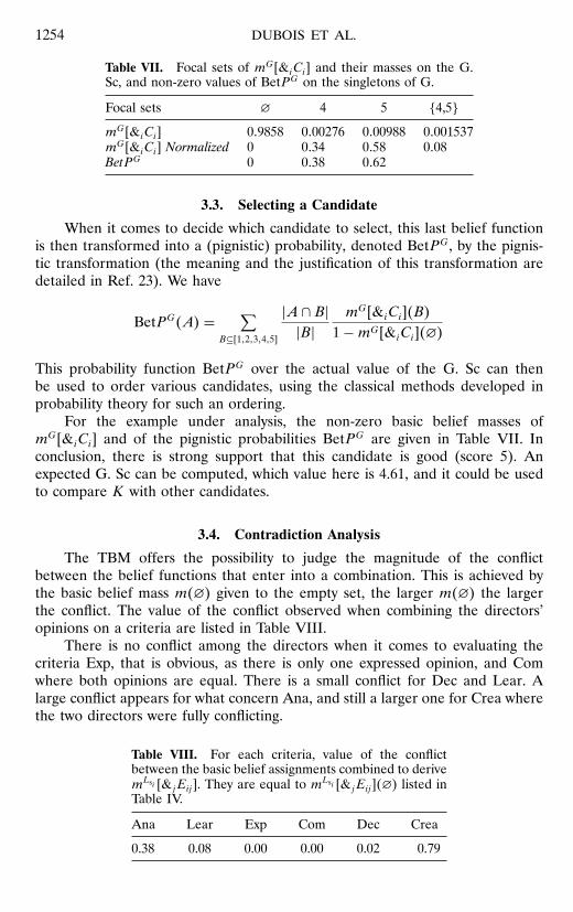
3.4. Contradiction Analysis

The TBM offers the possibility to judge the magnitude of the conflictbetween the belief functions that enter into a combination. This is achieved bythe basic belief mass m� given to the empty set, the larger m� the largerthe conflict. The value of the conflict observed when combining the directors’opinions on a criteria are listed in Table VIII.

There is no conflict among the directors when it comes to evaluating thecriteria Exp, that is obvious, as there is only one expressed opinion, and Comwhere both opinions are equal. There is a small conflict for Dec and Lear. Alarge conflict appears for what concern Ana, and still a larger one for Crea wherethe two directors were fully conflicting.

Table VIII. For each criteria, value of the conflictbetween the basic belief assignments combined to derivemLsi �&jEij �. They are equal to mLsi �&jEij �� listed inTable IV.

Ana Lear Exp Com Dec Crea

0.38 0.08 0.00 0.00 0.02 0.79


Table IX. For each ij , value of the mean G. Sc and their differ-ence with the observed score, when the imprecise Cij ’s take oneof the compatible precise values.a

Criteria Director Opinion Mean Score Difference

Lear Mkt 2 4'55 0'07Lear Mkt 3 4'62 0'00Lear Fin 1 4'61 0'00Lear Fin 2 4'57 0'04Lear Fin 3 4'58 0'03Lear Fin 4 4'65 0'03Lear Fin 5 4'66 0'04Lear HR 2 4'29 0'32Lear HR 3 4'47 0'14Lear HR 4 4'74 0'13Dec Mkt 1 4'61 0'00Dec Mkt 2 4'61 0'00Dec Mkt 3 4'61 0'00Dec Mkt 4 4'66 0'04Dec Mkt 5 4'70 0'08Dec Fin 1 4'61 0'00Dec Fin 2 4'61 0'00Dec Fin 3 4'61 0'00Dec Fin 4 4'65 0'03Dec Fin 5 4'68 0'06Dec Prd 1 4'61 0'00Dec Prd 2 4'61 0'00

aThe score are recomputed while keeping all Cij ’s unchanged exceptthe one considered.

The overall conflict computed when combining the basic belief assignmentson the G. Sc is 0.9858 (see Table VII). This conflict should convince the DMthat the opinions expressed by the directors are strongly conflicting and anyconclusion should be taken very cautiously as probably something went wrongsomewhere (as just happens to be the case when looking to the data for the Anaand Crea criteria).

3.5. Sensitivity Analysis

The TBM also allows us to perform a sensitivity analysis. We can considerwhat would be the final pignistic probabilities and the mean G. Sc if we hadobtained more precise assessments for each director and each criteria. Table IXlists the mean goodness scores one would have obtained if the various impreciseassessments had been precise, one by one. The considered values are consistentwith the collected intervals Cij . The largest difference, hence the largest sensitiv-ity, is observed for the data collected from the HR Director for the Lear criteria.So this is the first criteria that deserves to be assessed more precisely.

It is also possible to determine which data should be reconsidered in orderto reduce the conflicts. In the present example, it is obvious (see Table VIII) that

1256 DUBOIS ET AL.

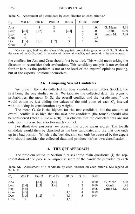
Table X. Assessment of a candidate by each director on each criteria.a

Cij Mkt D Fin D Prod D HR D G. Sc BetP

Ana 4 2 1 '00 G. Mean 4'61Lear [2,3] [1,5] 4 [2,4] 2 '00 Confl. 0'99Exp 4 3 '00 crude M. 3'08Com 4 4 4 '38Dec [1,5] [1,5] [1,2] 3 5 '62Crea 5 1

aOn the right, BetP are the values of the pignistic probabilities given to the G. Sc, G. Mean isthe mean of the G. Sc, confl. is the value of the overall conflict, and crude M. is the crude mean.

the conflicts for Ana and Crea should first be settled. This would mean asking thedirectors to reconsider their evaluations. This sensitivity analysis is not exploredfurther here as the problem is not at the level of the experts’ opinions pooling,but at the experts’ opinions themselves.

3.6. Comparing Several Candidates

We present the data collected for four candidates in Tables X–XIII, thefirst being the one studied so far. We tabulate the collected data, the pignisticprobabilities, the mean G. Sc, the overall conflict, and the “crude mean” onewould obtain by just adding the values of the mid point of each Cij intervalwithout taking in consideration any weight.

The mean G. Sc is the highest for the first candidate, but the amount ofoverall conflict is so high that the next best candidate (the fourth) should alsobe considered (mean G. Sc = 4.50). It is obvious that the collected data are notonly too imprecise but also too much conflict.

For illustrative purposes, we present the crude mean scores. The fourthcandidate would then be classified as the best candidate, and the first one endsup in a bad position. Which is the best decision can only be assessed by the expertwho should consider the collected data and produce his/her own classification.

4. THE QPT APPROACH

The problem stated in Section 2 raises three main questions: (i) the rep-resentation of the precise or imprecise score of the candidate provided by each

Table XI. Assessment of a candidate by each director on each criteria. See legend ofTable X.


Ana [2,4] [1,4] 1 0'00 G. Mean 3'98Lear [2,4] [1,3] [1,4] 2 2 0'00 Confl. '91Exp [4,5] 3 0'06 Crude M. 3'13Com [4,5] [4,5] 4 0'89Dec [1,3] [1,2] 4 [4,5] 5 0'04Crea 3 [4,5]


Table XII. Assessment of a candidate by each director on each criteria. See legend ofTable X.


Ana 4 [2,3] 1 '00 G. Mean 3'44Lear [2,3] [2,4] 5 [2,4] 2 '00 Confl. '82Exp [3,4] 3 '61 Crude M. 3'08Com [2,4] [1,4] 4 '33Dec [3,5] 1 3 [2,4] 5 '05Crea [3,5] 3

expert for each criterion, including the expert’s confidence in his assessment; (ii)the fusion of expert opinions; (iii) the multiple criteria aggregation. The first stepis easily handled in qualitative possibility theory14 which offers a representationframework for handling imprecise values pervaded with qualitative uncertainty.This might be related to the processing of fuzzy marks for students’ evaluationfor which an (ad hoc) treatment was proposed recently.2 An alternative wouldhave been to map the ordinal scale on a suitable cardinal scale by a method suchas “Macbeth.”3 However this approach requires additional information.

In the following, ∨ and ∧ denote max and min on a given ordinal scale.¬x for any x in a given ordinal scale L = �� s1� � � � � sk� � denotes the valuecorresponding to the reversed scale (i.e., ¬� = ��¬si = sk−i+1). It is the counter-part to 1− x on the �0� 1� interval scale. To simplify the notation we have denotedthe top and bottom elements of each scale by the same symbols; however thisdoes not mean that they are the same.

4.1. Representing Imprecise and Uncertain Scores

The evaluation of each criterion for candidate K and a given expert j maybe imprecise (either due to the fact that it is unclear to what precise extentK satisfies criterion i� or due to the possible lack of competence in i of theexpert j assessing the value). Each evaluation will be represented by a possibilitydistribution (discounted in case of limited expertise) restricting the more or lesspossible values of this evaluation. Let �j

ciK(�j

i for short) denote the possibilitydistribution restricting the possible values of ciK according to expert j .

Table XIII. Assessment of a candidate by each director on each criteria. See legend ofTable X.


Ana [4,5] [1,5] 1 '00 G. Mean 4'50Lear [1,3] [4,5] 4 [2,3] 2 '00 Confl. '75Exp [4,5] 3 '03 Crude M. 3'21Com [3,5] [2,4] 4 '44Dec [1,3] [4,5] 3 [2,3] 5 '53Crea [1,5] [1,5]

1258 DUBOIS ET AL.

Table XIV. Opinions of directors on each criterion after fuzzifi-cation and discounting.

Mkt D Fin D Prod D HR D

Ana �� a�a a�a�� Lear a��aa �� aaa�a a��aExp ��a�a �� Com ��a�a �� a�aDec �� bbb bb�bbCrea ��a� �� a��

The possibility distribution (�.d.f. for short) of the true value of each scoreon criterion i according to expert j , taking into account his competence, is com-puted in the following way. Interval-valued scores (including single values) aremodeled by a possibility distribution taking the value � in the interval and �outside. Blanks (absence of answers) are interpreted as a possibility distributionbeing � everywhere (modeling “unknown”). The confidence level �ij is taken intoaccount by a discounting process, defined as (�̃ denotes the original possibilitydistribution function)

�ji s = �̃

ji s ∨ ¬�ij ∀s ∈ Ls (5)

Note that the certainty level �ij ∈ L� is turned into a possibility level ¬�ijover the scores not compatible with �̃j

i . Thus L� is L� reversed (this is the usualequivalence between certainty of A and impossibility of not A).

Moreover, as in the TBM approach (Section 3.1), it is admissible here tofuzzify the measurements of each director, because the score scale {1,2,3,4,5}may be thought of as a discretized continuum, which means, e.g., that 3 is closeto 4 in some sense, as when a director says “4” we cannot fully exclude neither3 nor 5. We use the same fuzzification as in Section 3.1, except that the valuesimmediately close to the assessments receive the possibility “a” (instead of 0.5 asin Section 3.1, values which are further away remain with a zero possibility. Thisfuzzification takes place before applying expression (5). Thus �̃j

i should be thefuzzified original possibility distribution in expression (5). This fuzzification andthe discounting lead to Table XIV. In each cell the �.d.f. is enumerated on Ls.

4.2. Merging Expert Opinions

As already stated, the global assessment requires two types of combination:a multiple-criteria aggregation problem, and the fusion of expert evaluations. So,depending on the way the problem is presented, we may either think of (i) firstcomputing the global evaluation of K according to each expert and then to fusethese evaluations into a unique one, or (ii) on the contrary, first fuse the expertevaluations for each criterion, and then aggregate the “global” results pertainingto each criterion. In general, the two procedures are not equivalent (i.e., expertopinion fusion and multiple-criteria aggregation do not commute, and the same


holds for the TBM analysis). So it is important to understand what is the mean-ingful order between the fusion and aggregation operations, or if this remainsunclear, to choose fusion and aggregation modes which commute.

At this point, it is worth emphasizing that expert opinion fusion and multiplecriteria aggregation are two operations which do not convey the same intendedsemantics. The fusion of expert opinions aims at finding out what are the possiblevalues of the genuine score of K for a given criterion, and possibly to detectconflicts between experts. Hopefully, some consensus should be reached at leaston values which are excluded as possible values of the score. The aggregation ofmultiple-criteria evaluations aims at assessing the global worth of the candidatefrom his scores on the different criteria; then different aggregation attitudesmay be considered, e.g., conjunctive ones where each criterion is viewed as aconstraint to satisfy to some extent, or compensatory ones where trade-offs areallowed.

In the following, we choose to merge expert’s opinions on each criterionfirst, and then to perform a multiple-criteria aggregation, since it might seemmore natural to use the experts first to properly assess the score according toeach criterion. Proceeding in the other way would assume that each expert islooking for a global evaluation of the candidate (may be using his own criteriaaggregation attitude) and the decision maker is only there for combining andweighting expert’s evaluations.

Let us first merge the distributions pertaining to a single criterion. Whenthere is no major conflict between the assessments to be merged, a conjunctivecombination can be performed which singles out values of common agreement.In QPT, possibility distributions are then combined by the min operation (heredenoted ∧), after having been discounted if necessary. When there is a strongconflict, i.e., here when

for some i� conflicti =∨s

∧j

�ji s = 0� (6)

disjunctive combination is advisable in such a case§ (see Ref. 10). Conjunctivefusion can be applied only if there is no conflict in the above sense. A disjunctivecombination means that the opinion of an important expert will not be forgot-ten, even if it conflicts with another important one. See Ref. 10 for a generalintroduction to the logical view of information fusion and its encoding in thepossibilistic framework by weighted conjunctions and disjunctions.

However, unreliable estimates should be discounted both in the conjunc-tive and in the disjunctive merging. The reliability wij attached to �j

i should beboth upper bounded by the confidence �j of DM in the expert j and the self-confidence �ij of the expert. This leads to take the weight wij as the conjunctive-like combination of �j and �ij ∀i = 1� � � � � 6.

§Here we assume that a conflict occurs when the intersection of �.d.f.’s is empty.Note that since the underlying space is ordered, and a fuzzification has been performedat the previous step, conflicts are less often present (however one still occurs for criteriai = 6 (Crea)).

1260 DUBOIS ET AL.

Table XV. Definition of ⊗.

⊗ � u v �

� � � � �a � a a ab � a b b� � a b �

The weighted conjunction, applied to i without conflict, will be

� ′i s =

∧j

[¬wij ∨ �j

i s]

∀s ∈ Ls' (7)

while the weighted disjunction is defined as

� ′i s =

∨j

[wij ∧ �j

i s]

∀s ∈ Ls� (8)

As said above, wij = �ij ⊗ �j , where ⊗ is a conjunction operator from L� ×L� to L� . Table XV defines ⊗ on the basis of an implicit commensuratenesshypothesis of L� and L�. Due to the idempotency of ∧ and ∨, the apparentlyredundant treatment of the information encoded by the �ij which are taken intoaccount both in expression (5), and in Eqs. 7 and 8 is innocuous for building thewij . Table XVI gives the weights for all criteria and experts.

In fact, it is not clear if the weights are absolute or relative. Here we haveassumed they are absolute. In case they are relative, we could use a “non-monotonic” conjunction or disjunction for discounting the part of the informationprovided by less important experts which is in conflict with what is provided bythe more important ones; see Ref. 10 for details.

We apply formula (7) to �.d.f.’s of Table XIV (or Eq. 8 if Eq. 6 holds).We obtain the �.d.f.’s of Table XVII (left). Moreover, in case of disjunctivecombination, translating the lack of answer of a director (here due to a total lackof competence) by the �.d.f. expressing total ignorance (possibility = 1 on eachscore) is not innocuous. Indeed, in case of disjunctive combination, assertingthe whole set {1� � � � � 5} amounts to state that the expert considers for some

Table XVI. Weights wij for all criteria anddirectors.

wij Mkt D Fin D Prod D HR D

Ana � a a �Lear b a a bExp � � � �Com � � � bDec a a a aCrea � � � b


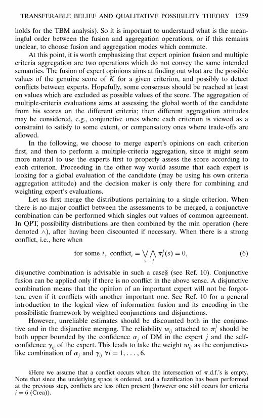
Table XVII. Merged opinions of directors on criteria; Merged opinions afternormalization.

Opinions on Criteria Opinions after Normalization

Ana aaaaa ��Lear abbaa b��bbExp ��a�a ��a�aCom ��a�a ��a�aDec bbbbb ��Crea ba�a� ba�a�

reason that the score can take any value in the set and that all of them areplausible: namely, the candidate is capable of the best as well as the worst w.r.t.the criterion. This is not the same as being fully ignorant about the candidate.So in Eq. 8, the scope of ∨ should be limited to the j ’s for which we have ananswer.

We notice that some distributions are no longer normalized (i.e., no score isfully possible at level �). In the case of the disjunctive combination, this is onlybecause the weights are not normalized, i.e., ∨jwij < � for some i’s, which meansthat the DM cannot be fully confident in any director for assessing some criteria(namely Ana, Lear and Dec). This is a little paradoxical, since it would be naturalthat the DM employs at least one fully reliable expert per criterion. In the caseof the conjunctive combination, resulting distributions are unnormalized in caseof partial conflicts. Thus, we should either use the unnormalized distributions tofully keep track of the problem, or normalize them in a suitable way. Here, wechoose the second solution, and propose the following approach. We considerthat the maximum of the distribution, denoted h, reflects the uncertainty level,considered to be ¬h in the information. This means that the amount of conflictis changed into a level of uncertainty and the minimum level of the modifieddistributions will be ¬h. Then, we make an additional hypothesis that the scaleis an interval scale (which is questionable) so that the profile of the distributionis not changed. Specifically

�is = � ′i s+¬

(∨s

� ′i s

)(9)

It means that + in Eq. 9 is defined by si + sj = smink+1� i+j on a scale �s0 =�� s1� � � � � sk� sk+1 = 1 . The result is shown in Table XVII. A slightly differentmethod would be to keep possibility degrees equal to � at �, since � ′

i s = �means that all experts agree on the fact that the value s is impossible.

Normalization has some advantage for the next step of the procedure. Due to theuse of the extension principle in the final step (see Eq. 12), we need to normalize, other-wise the resulting �.d.f. will be truncated by the height of the smallest distribution, andthus would continue to keep track of the lack of reliability of a part of the information,but would have its profile modified, since the nuances between more or less high degreesof possibility are lost.

1262 DUBOIS ET AL.

4.3. Criteria Aggregation

The way of aggregating the criteria evaluations is not at all specified in thestatement of the problem. The aggregation of preferences expressed by the crite-ria and their levels of importance is not viewed here as another multiple sourceinformation fusion problem as in Section 3 where the “goodness” of the candi-date was estimated by the conjunctive combination of the basic belief assignmentsmodeling the goodness of the candidate according to each criterion. In the fol-lowing the aggregation of criteria is viewed as a problem different from datafusion, where we are not trying to estimate the true value of a parameter, butrather to express how the levels of satisfaction of each criterion contribute to theglobal level of satisfaction, just allowing for trade-offs. However the aggregationfunction (which is not at all part of the QPT model) is almost unspecified here.Moreover, the evaluations attached to each criterion are not pointwise here, butrather imprecise and pervaded with uncertainty.

Only qualitative levels of importance �i are provided for each criterion i.Even with ordinal scales, different attitudes can be thought of. The aggregationmay be purely conjunctive (based on weighted “min” operation), or somewhatcompensatory (using a median operation for instance). It might be also disjunc-tive if at least one important criterion has to be satisfied, then it is modeled bya weighted maximum. More general aggregation attitudes can be captured bySugeno’s integral.17�25 Let us assume that the DM has somehow a compensatoryattitude.

Here we use the only associative qualitative compensatory aggregation oper-ator, namely the median. Indeed, minx� y ≤ medianx� y� � ≤ maxx� y forany � belonging to the domain of x and y. Thus we shall take � to be the middlepoint of the scale, i.e., 3, since it will be applied to Ls = �1� 2� 3� 4� 5 ; Due to itsassociativity, the median operation can be easily generalized to the aggregationof n terms, namely median (x1� x2� �) becomes median (

∧k xk�

∨k xk� �). How-

ever we have still to take into account the importance levels of the criterion. Sothe global score s after aggregation will be taken to be equal to median c� d� �)where c (resp. d) is a weighted conjunction (resp. disjunction) computed as fol-lows.

With our notations, in the case of precise scores, the global score combina-tion with the weighted minimum method is obtained by:

c =6∧i=1

�¬�i∨̃ci� (10)

where ∨̃ is a disjunctive operator from L� ×Ls to Ls. Table XVIII, part(a), givesthe definition of this operator.

Computed with the weighted maximum, the global score would be:

d =6∨i=1

��i∧̃ci� (11)

where ∧̃ is given in part(b) of Table XVIII.


Table XVIII. Definition of ∨̃ and ∧̃.

� e f g 1

(a) Disjunctive Operator ∨̃1 1 2 3 4 52 2 2 3 4 53 3 3 3 4 54 4 4 4 4 55 5 5 5 5 5

(b) Conjunctive Operator ∧̃1 1 1 1 1 12 1 2 2 2 23 1 2 3 3 34 1 2 3 4 45 1 2 3 4 5

The “fuzzy” evaluations provided by the �.d.f.’s should now be aggregated.A natural manner to proceed is to extend multiple-criteria aggregation tech-niques to such non-scalar evaluations (this can be done both if this step is donebefore or after the fusion step). At the technical level, this is done using anextension principle27 which makes it possible to extend any function/operation fto any fuzzy arguments. Namely,

f �1� � � � � �ms =∨

s=f s1� � � � �sm�1s

1 ∧ � � � ∧ �msm

where �isi is the possibility degree of score si according to �.d.f. �i.Here f is the aggregation function f c1� � � � � c6� �1� � � � � �6 = median

c� d� 3. We have for any s ∈ Ls and candidate K,

�Ks =∨

s=median3�∧6i=1�¬�i∨̃ci��

∨6i=1��i∧̃ci�

�1c1 ∧ · · · ∧ �6c6 (12)

Applying this formula to our data, we finally obtain the distribution given inTable XIX.

The result can be interpreted by saying that the candidate K is certainlynot a very good candidate nor a bad or average one, and K is between mediumand good. Let us briefly comment the result. The most important criteria areCom and Crea, where the scores are, respectively, 4 and 1 or 5 (with possibility�). This explains why the global value 5 is impossible, since it is not reached byone important criterion. Moreover the score on criterion Dec which is rather

Table XIX. Possibility distribution �K of thefinal score.

Score 1 2 3 4 5

Possibility degree � � � � �

1264 DUBOIS ET AL.

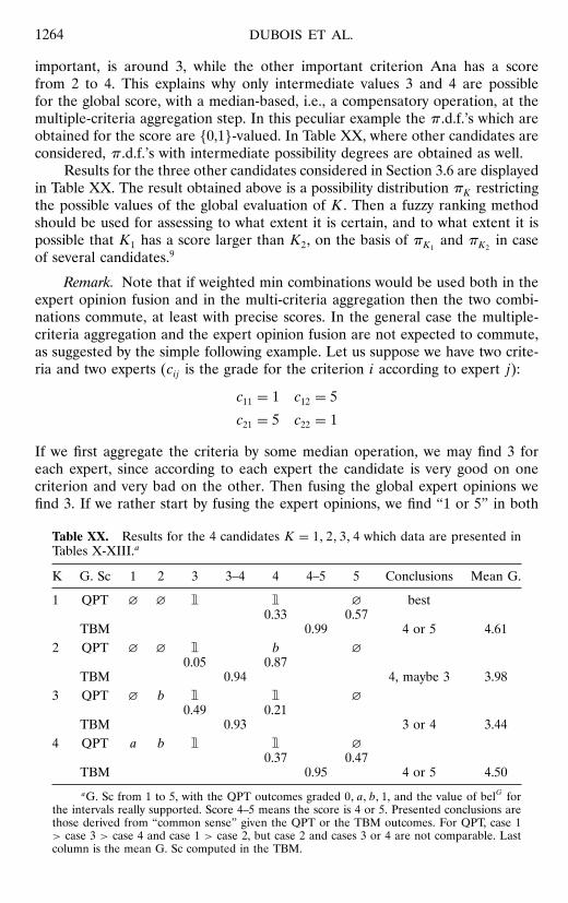
important, is around 3, while the other important criterion Ana has a scorefrom 2 to 4. This explains why only intermediate values 3 and 4 are possiblefor the global score, with a median-based, i.e., a compensatory operation, at themultiple-criteria aggregation step. In this peculiar example the �.d.f.’s which areobtained for the score are {0,1}-valued. In Table XX, where other candidates areconsidered, �.d.f.’s with intermediate possibility degrees are obtained as well.

Results for the three other candidates considered in Section 3.6 are displayedin Table XX. The result obtained above is a possibility distribution �K restrictingthe possible values of the global evaluation of K. Then a fuzzy ranking methodshould be used for assessing to what extent it is certain, and to what extent it ispossible that K1 has a score larger than K2, on the basis of �K1

and �K2in case

of several candidates.9

Remark. Note that if weighted min combinations would be used both in theexpert opinion fusion and in the multi-criteria aggregation then the two combi-nations commute, at least with precise scores. In the general case the multiple-criteria aggregation and the expert opinion fusion are not expected to commute,as suggested by the simple following example. Let us suppose we have two crite-ria and two experts (cij is the grade for the criterion i according to expert j):

c11 = 1 c12 = 5

c21 = 5 c22 = 1

If we first aggregate the criteria by some median operation, we may find 3 foreach expert, since according to each expert the candidate is very good on onecriterion and very bad on the other. Then fusing the global expert opinions wefind 3. If we rather start by fusing the expert opinions, we find “1 or 5” in both

Table XX. Results for the 4 candidates K = 1� 2� 3� 4 which data are presented inTables X-XIII.a

K G. Sc 1 2 3 3–4 4 4–5 5 Conclusions Mean G.

1 QPT � � � � � best0.33 0.57

TBM 0.99 4 or 5 4.612 QPT � � � b �

0.05 0.87TBM 0.94 4, maybe 3 3.98

3 QPT � b � � �0.49 0.21

TBM 0.93 3 or 4 3.444 QPT a b � � �

0.37 0.47TBM 0.95 4 or 5 4.50aG. Sc from 1 to 5, with the QPT outcomes graded 0� a� b� 1, and the value of belG for

the intervals really supported. Score 4–5 means the score is 4 or 5. Presented conclusions arethose derived from “common sense” given the QPT or the TBM outcomes. For QPT, case 1> case 3 > case 4 and case 1 > case 2, but case 2 and cases 3 or 4 are not comparable. Lastcolumn is the mean G. Sc computed in the TBM.


cases, since they are conflicting. Note that the result will be the same at this stepfor the following very different data set:

c11 = 16 c12 = 5'

c21 = 16 c22 = 5'

We have just forgotten, when we will apply some extended aggregation operationto “1 or 5” and “1 or 5” that the pairs (1, 1) and (5, 5) are impossible (with thefirst set of data).

4.4. Qualitative Expected Values

The assessment problem can be viewed as a decision to be made underuncertainty. Namely, the relevance of the criteria defines a candidate profile, i.e.,a kind of utility function, while the value of the candidate K is ill-known withrespect to each criterion (once expert opinions have been fused). Viewing theproblem in this way, it is natural to compute to what extent it is certain (or itis possible) that the candidate K (whose level assessment may be pervaded withimprecision and uncertainty for each criteria) satisfies the criteria at the requiredlevel; see Ref. 12 for an axiomatic view of the corresponding qualitative decisionprocedure. In practice, it corresponds to a fuzzy pattern matching problem.6

For each criterion i, we build a satisfaction profile 7i, e.g., 7is = ¬�i ∨s. 7i means that the greater the score, the better the candidate, and that thesatisfaction degree is lower bounded by ¬�i which is all the greater as i is lessimportant. Then the certainty that K satisfies the profile is given by

∧i

∧s

7is ∨ ¬�ciKs (13)

where �ciK is supposed to be normalized. The possibility that K satisfies theprofile is

∧i

∨s

7is ∧ �ciKs (14)

where �ciK has been obtained by fusing the expert opinions first, at the level ofeach criterion. The possibility degree (very optimistic) should be only used forbreaking ties in case of equality of the certainty degrees for different candidates.The aggregation by

∧i of the elementary certainty and possibility degrees can be

justified in the possibility framework (definition of a join possibility distribution ofnon-interactive variables,27 when the global requirement is interpreted in terms ofa weighted conjunction of elementary requirements pertaining to each criterion).The expressions (13) and (14) can be viewed as possibilistic “lower and upperexpectations.”

When a median-based aggregation is used, the possibility and the necessitymeasures are no longer

∧i-decomposable as in expressions (13) and (14) and we

1266 DUBOIS ET AL.

would have to compute directly the possibility and the necessity that the globalsatisfaction profile (again computed from the 7i by application of the extensionprinciple) is satisfied giving the joint �.d.f.

∧i �CiK.

What is computed remains in the spirit of the approach detailed before.Instead of obtaining a possibility distribution we obtain two scalar evaluationsfor which it should be possible to show that they summarize this possibility dis-tribution (in a sense to be made precise at the theoretical level). Anyway bothapproaches first compute the �ciK’s and are based on the choice of an aggrega-tion function.

Note also that we are not obliged to combine the different evaluations �ciKpertaining to each criterion (once we have fused the expert grades). We maysummarize each possibility distribution by a “lower expected value,” and thencompare lexicographically tuples made of the scalar evaluations thus obtainedfor each criterion (the scalar evaluations being ordered in the tuple according tothe importance of the criteria), for different candidates.

5. GENERAL DISCUSSION

The use of the two approaches for dealing with the same (class of) prob-lems has raised two types of issues which are now briefly considered; namelyfirst a comparison of the approaches, and second how each approach could bevalidated.

5.1. Outline of a Comparison

The reader may observe some agreement between the results obtained bythe belief function approach and by the possibilistic approach, when consid-ering the possibility distributions and the mass functions which are obtained,before computing the expected values (see Table XX). This is not too surprisingif we consider the two flowcharts summarizing the two approaches, which arerather similar (see Tables XXI and XXII). However the remaining discrepanciesbetween results are largely due to the different views which are chosen at themultiple-criteria aggregation step.

In QPT-based approach, merging opinions and aggregating criteria are envis-aged as two different problems. Merging opinions is performed by min-basedcombination of the �.d.f.’s, as prescribed by QPT, when there is no conflict. Whena conflict exists, it means that at least one of the opinions is totally wrong, anda max-based disjunction is performed in order to save the provided information.Then the weighting of the conjunction or of the disjunction amounts to a prelim-inary discounting or truncation of the �.d.f.’s according to the confidence in thesources. Aggregating criteria supposes to know if trade-offs exist or not. Thereexists a large panoply of different possible aggregation attitudes, even when deal-ing with qualitative scales. This contrasts with the view used in the TBM-basedapproach where only Dempster rule of combination, which is conjunctive, is usedhere. However, belief functions viewed as set functions could have been usedfor describing multiple-criteria aggregations based on Choquet integrals, where


sets of criteria can be weighted.18 In case other aggregation operations would bechosen at the multiple criteria aggregation step, with the QPT approach, resultswhich are rather different could be obtained. For instance, choosing a weightedmin-combination at the aggregation step, would lead to results where low scoreswould not be excluded (see Table XXIII for the results which would be obtainedfor the first candidate).

The other discrepancies between the results obtained in Sections 3 and 4with the two approaches may have several reasons.

• The QPT approach using a qualitative possibility scale cannot use any direct coun-terpart of the product used in the TBM approach. Moreover using the possibilitytheory approach with a [0,1] scale will open the door to the use of adaptativemerging operators11 which provide a softer adaptation between the conjunctiveand the disjunctive attitudes (using the degree of conflict as a weighting factor).

• Moreover, when introducing the G. Sc in the belief function approach, the under-lying idea is that we are all the less demanding for reaching the maximum level ofsatisfaction as the criterion is less important. This is not the understanding cho-sen in the possibilistic approach (remember that the problem is not completelyspecified). Rather, the unimportant criteria were considered as somewhat satisfiedeven if they were not at all satisfied. In fact there are different possible ways ofunderstanding the weighting of the criteria, in a qualitative conjunctive setting.

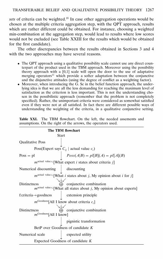
Table XXI. The TBM flowchart. On the left, the needed assements andassumptions. On the right of the arrows, the operators used.

The TBM flowchartStart

Qualitative Poss�

Poss(Expert says Cij � actual value ci)

Poss = pl� PossA�B = pl�B�A = pl�A�B

mactual value ci [What expert i states about criteria j]

Numerical discounting� discounting

mactual value ci [What i states about j , My opinion about i for j]↘↓↙

Distinctness⊕

conjunctive combinationmactual value ci [What all states about j , My opinion about experts]

f:criteria→goodness� extension principle

mGoodness[All I know about criteria ci]↘↓↙Distinctness

⊕conjunctive combination

mGoodness[All I know]� pignistic transformation

BetP over Goodness of candidate K

Numerical scale� expected utility

Expected Goodness of candidate K

1268 DUBOIS ET AL.

Table XXII. The QPT flowchart. On the left, the needed assessments andassumptions. On the right of the arrows, the operators used.

The QPT flowchartStart

Qualitative Possibilities� representation of fuzzified data

Poss(actual value ci � Expert says Cij)

Qual. opinion on i for j� discounting

Poss(actual ci � Expert says Cij , My opinion about i for j)↘↓↙

Merging expert opinions: weighted min (max if conflict)

Disj. combi. if conflict�

Normalization of merged opinions

Define aggregation rule� extension principle on median-based aggregation.

Satisfaction pattern : Poss (score � All I know & aggregation rule)�Optimistic and pessimistic expectations about global value of K.

Let ciK be the supposedly precise value of score of K, according to criterion i.Indeed, we can (i) modify ciK into ¬�i∨̃ciK as we did, or (ii) modify ciKinto

{5 if ciK ≥ �i

ciK if ciK < �i

(�i is interpreted as a threshold level to reach in order to be fully satisfied, takingadvantage of the commensurateness hypothesis underlying Table XVIII), (iii) orwe may even think of ¬�i as a “bonus” to be added to ciK. Once the type ofweighted conjunction has been chosen, it has to be extended to the �.d.f.’s �i,since the precise value of ciK is not available. Choosing the option (ii) above inthe QPT approach instead of (i) would be similar to the idea of G. Sc as definedin the TBM approach.

• The value assessment problem considered here is probably not the best type ofexample for exhibiting the benefit of one of the specificities of the TBM approach,namely the capability of putting masses on subsets of values which are not single-tons. More generally, this capability might be of interest both at the merging stepand at the aggregation step (then leading to a Choquet integral-based evaluationas already mentioned).

The example also raises the issue of the difference between a value assertedby the expert as “unknown” (interval [1, 5] in the example), and the absence

Table XXIII. Possibility distribution � of the final score.

Score 1 2 3 4 5

Possibility degree b � � � 0


of answer by the expert for a criterion evaluation. Even if in both cases, theresult is that the evaluation is actually unknown, the reason for the absence ofan answer may be either that the director feels himself totally incompetent anddoes not answer (as already discussed), or that the criterion does not really applyto Mr. K (according to the expert). This will call for a richer evaluation frame-work where the evaluation assessment can take its value in an extended domain�1� 2� 3� 4� 5 ∪ �does_not_apply . Then it creates further difficulties, especiallywhen comparing candidates.

For summarizing the main differences between the belief function (TBM)and the possibility-based approaches (QPT) on the value assessment problem,it is clear that the possibilistic method can handle poor data expressed in aqualitative, non-numerical, way whereas the belief function framework may moreeasily capture reinforcements and compensatory effects. In the QPT approach,the propagation of imprecision and uncertainty in the combination process hasbeen emphasized, while the TBM approach has privileged the decision step bycomputing expected values.

5.2. Brief Discussion on the Validation Issues

The validation of an approach used in practice involves several aspectsaccording to which an approach may be judged and compared to others.

A first type of validation is the practical one (not always easy to perform).It consists in checking the “correctness” of the results provided by the systemby comparing them to those produced by a panel of experts (w.r.t. to the infor-mation actually provided to the system). One must nevertheless be careful thatthe experts might not provide a golden standard. This approach produces ameasure of concordance between two systems, not always a measure of quality.Furthermore a system may provide correct results without being considered asgenuinely “useful” by the experts. Anyway this type of validation is usually doneon systems which are already developed at an operational level. The real prag-matic validation should be carried on as it is done in medicine, through a clinicaltrial where several methods are compared on many real examples and their val-ues assessed by comparing the final results.

But other aspects should also be considered first. In the following we dis-tinguish between those pertaining to normative, empirical, computational andexplanatory issues.

From a normative validation point of view, we can see our problem asmade of two main steps: (i) the combination of pieces of information com-ing from different experts, (ii) then a decision step made on the basis of theimprecise/uncertain information obtained at the end of step i with respect to a(multiple criteria) value function, as pointed out at the end of Section 4. “Nor-mative” refers to the existence of postulates which, once accepted, necessarilylead to a specific method. Regarding the combination of uncertain information,there are no genuine normative approaches available although there exist char-acterization theorems in various frameworks. Thus the min-based combination

1270 DUBOIS ET AL.

is the only conjunctive idempotent attitude, whereas Dempster’s rule of combi-nation is not idempotent (even though there exist other combination rules thatare more cautious and idempotent). Concerning the decision step, the situa-tion is a bit different since there exist well-established normative frameworks.Regarding decision under uncertainty, one has been recently proposed for vonNeumann–Morgensten and Savage-like justifications of the possibility theory-based approach.12�15 For the TBM, the pignistic transformation produces a prob-ability used for decision making; its justification is detailed in Ref. 23 and theavoidance of any Dutch-book is explained in Ref. 22.

Regarding empirical validation, we face a cognitive problem. Is the repre-sentation framework used cognitively meaningful? Are the operations performedon the representation meaningful? Preliminary (positive) elements of answersconcerning the possibility theory framework can be found in Ref. 19.

Concerning the computational issue, the two methods presented are clearlycomputationally manageable in practice (even if one is simpler). The fact thatDempster’s rule of combination is NP complex is not a real issue here as thekind of data expected are simple and the involved belief functions have fewcomponents, making the computation tractable in practice.

Finally, it is also important to judge the (potential) explanation capabilities.Are the results provided by the system easy to explain to the user if necessary?For example, why the value of the candidate is finally assessed as such? Suchexplanation capabilities are presented in Ref. 16 and in Ref. 26 for the QPT andthe TBM, respectively. Generally, the qualitative framework of possibility theoryallows for a logical reading and processing of the evaluations.1�5

6. CONCLUDING REMARKS

In this paper, we have taken advantage of a generic value assessment prob-lem for discussing the different facets of the problem and raising the variousdifficulties and hypotheses which should be made at each step for computing ameaningful evaluation through two models, the QPT and the TBM.

The purpose of the paper was twofold: first identifying and discussing variousfacets of a value assessment problem, and second showing how two differentapproaches (which have in common the capability of modeling imprecision) canhandle the problem in ways which are in fact quite parallel.

The statement of the problem contains no numerical data, but only ordi-nal assessments. Owing to the qualitative framework of possibility theory, theQPT provides a natural approach. However note that it is important to considerthe nature of the scales which are used in order to know what operations aremeaningful on them. Moreover commensurateness hypotheses are necessary.

With the TBM, numbers (the beliefs) are needed. They are in fact analogousto those for which a probability approach would ask. The difference betweenthe TBM and a probability approach is that the TBM accepts and uses the datajust as they are, without introducing extraneous data. For example, a probabilityapproach would allocate (equal) probabilities to each of the individual values ofthe scores when the score is only known as a non-degenerate interval.


Sensitivity analysis can be performed, where either the values of the param-eters (TBM) or the aggregation operators (QPT) are slightly modified and therobustness of the conclusions can be assessed. Furthermore the DM can alsodetermine the sensitivity of the results if more precise data were collected. Giventhis information, the DM could efficiently ask a specific expert to provide a betterestimate of the candidate score for a specific criterion, avoiding getting “useless”data.

Special thanks are due to Simon Golstein who helped in stating the candidate valueassessment problem considered in this paper. The authors are indebted to Patrice Pernyfor valuable comments on the meaning of the absence of commutation of the multiplecriteria aggregation and the expert opinion fusion operations.

References

1. Benferhat S, Dubois D, Prade H. From semantic to syntactic approaches to informa-tion combination in possibilistic logic. In: Bouchon-Meunier B, editor. Aggregationand fusion of imperfect information. Heidelberg: Physica-Verlag; 1997, p 141–161.

2. Biswas R, An application of fuzzy sets in student’s evaluation. Fuzzy Sets Syst1995;74:187–194.

3. Bana e Costa CA, Vansnick J-C. A theoretical framework for measuring attractivenessby a categorical based evaluation technique (MACBETH). In: Proceedings of theXIth Int. Conf. on MCDM, Coimbra, Portugal, 1994, p 15–24.

4. Club CRIN Logique Floue. Evaluation subjective—Méthodes, applications et enjeux.Association ECRIN, 32 bd de Vaugirard, 75015 Paris.

5. Dubois D, Prade H, Sabbadin R. A possibilistic logic machinery for qualitative deci-sion. In: Proceedings of the AAAI’97 Spring Symposium Series on Qualitative Pref-erences in Deliberation and Practical Reasoning, Stanford, CA, 1997, p 47–54.

6. Dubois D, Prade H, Testemale C. Weighted fuzzy pattern matching. Fuzzy Sets Syst1988;28(3):313–331.

7. Dubois D, Grabisch M, Prade H. Assessing the value of a candidate. A qualita-tive possibilistic approach. In: Symbolic and Quantitative Approaches to Reasoningand Uncertainty Proc. (ECSQARU 99), LNAI 1638, Berlin: Springer Verlag, 1999,p 137–147.

8. Dubois D, Grabisch M, Prade H, Smets P. Assessing the value of a candidate. Com-paring belief functions and possibility theories. In: Proceedings of the XVth Confer-ence, Uncertainty in Artificial Intelligence, San Francisco: Morgan Kaufmann; 1999,p 170–177.

9. Dubois D, Prade H. Ranking fuzzy numbers in the setting of possibility theory, InformSci 1983;30.

10. Dubois D, Prade H. Possibility theory and data fusion in poorly informed environ-ments. Contr Eng Prac 1994;2(5):811–823.

11. Dubois D, Prade H, Decision making under fuzzy constraints and fuzzy criteria–mathematical programming versus rulebased approach. In: Delgado M, KacprzykJ, Verdegay JL, Vila MA, editors. Fuzzy optimization–recent advances. Heidelberg:Physica-Verlag; 1994, p 21–32.

12. Dubois D, Prade H. Possibility theory as a basis for qualitative decision theory. In:Proc. of the 14th Int. Joint Conf. on Artificial Intelligence (IJCAI’95), Montréal,Canada, 1995, p 1924–1930.

13. Dubois D, Prade H. Fuzzy criteria and fuzzy rules in subjective evaluations—A generaldiscussion. In: Proceedings of the 5th European Congress on Intelligent Technologiesand Soft Computing (EUFIT 97), Aachen, Germany, 1997, p 975–978.

1272 DUBOIS ET AL.

14. Dubois D, Prade H. Possibility theory: Qualitative and quantitative aspects. In: SmetsPh, editor. Quantified representation of uncertainty and imprecision. Handbook ofdefeasible reasoning and uncertainty management systems. Gabbay DM, Smets Ph,series editors. Dordrecht: Kluwer Academic Publishers; Vol. 1, 1998, p 169–226.

15. Dubois D, Prade H, Sabbadin R. Qualitative decision theory with Sugeno integrals.In: Proc. of the 14th Conf. Uncertainty in Artificial Intelligence (UAI’98), Madison,USA, 24–26 July 1998, Morgan Kaufmann, Los Altos, CA, p 121–128.

16. Farreny H. Prade H. Positive and negative explanations of uncertain reasoning in theframework of possibility theory. In: Zadeh LA, Kacpryk J, editors. Fuzzy logic for themanagement of uncertainty. New York: Wiley; 1992, p 319–333.

17. Grabisch M, Nguyen HT, Walker EA. Fundamentals of uncertainty calculi with appli-cations to fuzzy inference. Dordrecht: Kluwer Academic Publishers; 1995.

18. Grabisch M, Roubens M. Application of the Choquet integral in multiattribute deci-sion making. In: Fuzzy measures and integrals. Theory and applications. Heidelberg:Physica-Verlag; 2000, p 348–374.

19. Raufaste E, Rui Da Silva Neves. Empirical evaluation of possibility theory in humanradiological diagnosis. In: Proc. of the 13th Eur. Conf. on Artificial Intelligence(ECAI’98), Brighton, UK, New York: Wiley, 1998, p 124–128.

20. Shafer G. A mathematical theory of evidence. Princeton, NJ: Princeton UniversityPress; 1976.

21. Smets P. Belief functions: The disjunctive rule of combination and the generalizedBayesian theorem. Int J Approx Reason 1993;9:1–35.

22. Smets P. No Dutch Book can be built against the TBM even though update is notobtained by Bayes rule of conditioning. In: Scozzafava R, editor. SIS, Workshop onProbabilistic Expert Systems, Roma, 1993, p 181–204.

23. Smets P, Kennes R. The transferable belief model. Artificial Intell 1994;66:191–234.24. Smets P. The transferable belief model for quantified belief representation. In: Gabbay

DM, Smets Ph, editors. Handbook of defeasible reasoning and uncertainty manage-ment systems. Vol. 1, Dordrecht: Kluwer Academic Publishers; 1998, p 267–301.

25. Sugeno M. Fuzzy measures and fuzzy integrals: A survey. In: Fuzzy automata anddecision process. Amsterdam: North-Holland; 1977, p 89–102.

26. Xu H, Smets P. Some strategies for explanations in evidential reasoning explainingthe origin of a computed belief and finding which pieces of evidence are influencingthe results. IEEE Trans Syst Man and Cybernet 1996;26A:599–607.

27. Zadeh LA, The concept of a linguistic variable and its application to approxi-mate reasoning, Inform. Sci. Part 1, 1975;8:199–249; Part 2, 1975;8:301–375; Part 3,1975;1975:43–80.

using the transferable belief model and a qualitative possibility theory approach on an illustrative...

Documents