utilization of machine learning for flow assurance in …

1 | P a g e

UTILIZATION OF MACHINE LEARNING FOR FLOW ASSURANCE IN THE OIL

AND GAS SECTOR: A FOCUS ON ANNULAR FLOW PREDICTION

A thesis presented to the Department of Petroleum Engineering

African University of Science and Technology

In partial fulfilment of the requirements for the degree of

MASTER OF SCIENCE IN PETROLEUM ENGINEERING

By

Idris-Idah, Kawu Musa

Supervised by

Prof. Mukhtar Abdulkadir

African University of Science and Technology

www.aust.edu.ng

P.M.B 681, Garki, Abuja

F.C.T Nigeria

July, 2021

http://www.aust.edu.ng/

2 | P a g e

CERTIFICATION

This is to certify that the thesis titled “UTILIZATION OF MACHINE LEARNING FOR

FLOW ASSURANCE IN THE OIL AND GAS SECTOR: A FOCUS ON ANNULAR

FLOW PREDICTION” submitted to the school of postgraduate studies, African University

of Science and Technology (AUST), Abuja, Nigeria for the award of the Master's degree is a

record of original research carried out by IDRIS-IDAH KAWU MUSA in the Department of

Petroleum Engineering.

3 | P a g e

UTILIZATION OF MACHINE LEARNING FOR FLOW ASSURANCE IN THE OIL

AND GAS SECTOR: A FOCUS ON ANNULAR FLOW PREDICTION

By

Idris-Idah, Kawu Musa Idris-Idah

A THESIS APPROVED BY THE PETROLEUM ENGINEERING DEPARTMENT

RECOMMENDED: …… ……………

Supervisor, Prof. Mukhtar Abdulkadir

………………………………………………

Co-Supervisor,

………………………………………………

Co-Supervisor,

………………………………………………

Head, Department of Petroleum Engineering

APPROVED: ………………………………………………

Chief Academic Officer

……………………

Date

Alpheus

Stamp

4 | P a g e

© 2021

Idris-Idah, Kawu Musa

5 | P a g e

ALL RIGHTS RESERVED

6 | P a g e

ABSTRACT

There is insufficient literature for annular flow and applications of Machine Learning in the

petroleum industry; thus, this thesis is centred on annular flow prediction.

Liquid holdup and flow behaviour during annular flow was accurately predicted using the

Neural Network toolbox on MATLAB (Machine Learning). The experimental data contained

measurements of liquid holdup at three different probes across an air – water system, over a

period of 15 seconds. Measurements were noted at intervals of 0.001s; thus, a total number of

15,000 time steps. The superficial gas velocity within the system was changed 17 times

(ranging from 6.17 ms-1 to 16.05 ms-1), while the liquid superficial velocity was constant in all

cases (0.02 ms-1); data exists for 17 different velocities, for the 3 different probes.

Effective neural networks that yielded >90% validation accuracy were noted to occur when the

architecture was designed to have 10 hidden neurons and greater than 50 delays. An efficient

architecture was further solidified by analysis of the “Autocorrelation error” chart; all non-zero

lags should be within the confidence limit. This exceptional performance was ascertained via

the calculation of average liquid holdup values. The average liquid holdup of experimental and

simulated values was noted to be the same or greatly similar, proving accuracy of the

implemented neural network design.

This research has proved that the trend in annular flow time series data can be identified by a

neural network; further research could be carried out to determine the relevant variables that

are needed for accurate liquid holdup computations with time.

Keyword: Neural network, Flow Assurance, Liquid holdup.

7 | P a g e

ACKNOWLEDGEMENT

Written words will not do justice to my family’s sacrifice and support. I am forever grateful for

everything since “Day 1”, 29th of February 1996. It took a family, not a village, to deliver this

research. I especially can’t appreciate my father and mother’s contributions enough; I am

grateful.

My supervisor, Professor Mukhtar Abdulkadir, has been a blessing. Beyond your technical

contributions, your character is exemplary. I am grateful and extremely privileged to have been

supervised by the “King of Flow Assurance”.

I cannot say “Thank you” enough to my family in Maitama. I learnt a lot from you, and this

helped during this research work.

To my brothers in the United Kingdom and Kaduna; Adham El-Hossary, Hassan Abdi, Naveed

Hussain, Rayeed Anwar, Mukhtar Maigari, Mohammed Kalejaiye. We will meet again, some

day; In Shaa Allah.

Magnanimous appreciation for “The Francophonies” at AUST; every moment of joy and pain

with you has contributed towards the delivery of this research work. A team is better than an

individual.

Excessive gratitude to “Leeds Brothers”; you made the stressful moments seem less stressful.

It’s been more than seven years of exchanging ideas and dreams; we are forever strong.

Excessive gratitude to each and every person I met during my “French journey”; you improved

my competence and made me better. I am grateful.

I also acknowledge AUST for its scholarship; I am extremely grateful. The Head of

Department, Alpheus Igbokoyi, has been of monumental impact throughout my time at AUST.

To The Creator, I have reached this moment solely because of you. It is not by my

efforts, but by your mercy.

8 | P a g e

DEDICATION

This work is dedicated to everybody I have met, I will meet and those who I might not meet. I

hope this research further contributes towards the betterment of the world.

9 | P a g e

TABLE OF CONTENTS

CHAPTER ONE .................................................................................................................... 14

INTRODUCTION .............................................................................................................. 14

1.1. Preamble ............................................................................................................... 14

1.2. Problem Statement .............................................................................................. 16

1.3. Aims and Objectives ............................................................................................ 17

1.4. Research Justification ......................................................................................... 17

1.5. Scope ..................................................................................................................... 17

1.6. Organisation of Thesis......................................................................................... 18

CHAPTER TWO ................................................................................................................... 19

REVIEW OF MACHINE LEARNING LITERATURE ................................................ 19

2.1. Definition of Machine Learning ......................................................................... 19

2.2. Types of Machine Learning ................................................................................ 20

2.3. Machine Learning Algorithms ........................................................................... 21

CHAPTER THREE ............................................................................................................... 33

REVIEW OF FLOW ASSURANCE LITERATURE .................................................... 33

3.1. Definition of Multiphase Flow ............................................................................ 33

3.2. Important Concepts in Multiphase Flow........................................................... 33

CHAPTER FOUR .................................................................................................................. 48

METHODOLOGY ............................................................................................................. 48

4.1. Guo’s (2017) Method ........................................................................................... 48

4.2. Chollet’s (2017) Method ...................................................................................... 49

10 | P a g e

4.3. Developed method for Annular Flow. ................................................................ 50

CHAPTER FIVE .................................................................................................................... 58

RESULTS & DISCUSSION .............................................................................................. 58

5.1. Individual basis .................................................................................................... 66

5.2. Comparison basis ................................................................................................. 68

5.3. Average liquid holdup value basis ..................................................................... 70

5.4. Frequency basis.................................................................................................... 74

5.5. Structure velocity basis ....................................................................................... 75

CHAPTER SIX ...................................................................................................................... 76

CONCLUSION & RECOMMENDATIONS .................................................................. 76

6.1. Summary and Conclusions ................................................................................. 76

6.2. Recommendations ................................................................................................ 76

REFERENCES ....................................................................................................................... 78

11 | P a g e

LIST OF FIGURES

Figure 1 – Line of best fit ......................................................................................................... 22

Figure 2 – Decision Tree .......................................................................................................... 25

Figure 3 – ANN Architecture ................................................................................................... 30

Figure 4 – Annular Flow PDF .................................................................................................. 38

Figure 5 – Hewitt and Roberts Flow Pattern Map ................................................................... 39

Figure 6 – Taitel and Dicker Flow Pattern map ....................................................................... 40

Figure 7 – Griffith and Wallis Flow pattern map ..................................................................... 41

Figure 8 – Golan and Stenning’s Down-flow pattern map ...................................................... 42

Figure 9 - Golan and Stenning’s Up-flow pattern map ............................................................ 43

Figure 10 – Baker’s original flow pattern map ........................................................................ 45

Figure 11 - Baker’s modified flow pattern map ....................................................................... 45

Figure 12 – Whalley - Baker’s modified flow pattern map ..................................................... 46

Figure 13 – Developed method for Annular Flow prediction .................................................. 50

Figure 14 – Selection of NARX Solution ................................................................................ 53

Figure 15 – Importing Time Series Data ................................................................................. 54

Figure 16 – Neural network Architecture (1) ........................................................................... 54

Figure 17 – Splitting Time series dataset ................................................................................. 55

Figure 18 - Neural network Architecture (2) ........................................................................... 55

Figure 19 – Training Algorithm Selection ............................................................................... 56

Figure 20 – Plots Selection ...................................................................................................... 57

Figure 21 - Ug = 8.56 m/s, 9.42 m/s ........................................................................................ 60

Figure 22 - Ug = 13.25 m/s, 13.97 m/s .................................................................................... 60

Figure 23 - Ug = 8.56 m/s, 9.42 m/s ........................................................................................ 61

Figure 24 - Ug = 13.25 m/s, 13.97 m/s .................................................................................... 61

Figure 25 - Ug = 8.56 m/s, 9.42 m/s ....................................................................................... 62

12 | P a g e

Figure 26 - Ug = 13.25 m/s, 13.97 m/s .................................................................................... 62

Figure 27 - Ug = 14.63 m/s, 15.31 m/s .................................................................................... 63

Figure 28 - Ug = 14.63 m/s, 15.31 m/s .................................................................................... 63

Figure 29 - Ug = 14.63 m/s, 15.31 m/s .................................................................................... 64

Figure 30 - Ug = 13.97 m/s, 16.05 m/s .................................................................................... 64

Figure 31 - Ug = 13.97 m/s, 16.05 m/s .................................................................................... 65

Figure 32 - Ug = 13.97 m/s, 16.05 m/s .................................................................................... 65

Figure 33 – Time series (x = 8.1 m, Gas superficial velocity = 6.17ms-1)............................... 66

Figure 34 – Autocorrelation of Error 1 (x = 8.1 m, Gas superficial velocity = 6.17ms-1) ....... 67

Figure 35 – Best Validation performance (x = 8.1 m, Gas superficial velocity = 6.17ms-1) ... 67

Figure 36 – Liquid holdup against Gas superficial velocity .................................................... 73

Figure 37 – Crossplot of Experimental and Simulated frequencies ......................................... 74

Figure 38 - Crossplot of Experimental and Simulated Structure velocity ............................... 75

13 | P a g e

LIST OF TABLES

Table 1 – System Characteristics ............................................................................................. 39





Table 6 – Neural Network specifications for each gas superficial velocity ............................. 56

Table 7 – MSE and Epoch for each superficial velocity, at the first probe (x = 8.1 m) .......... 68

Table 8 - MSE and Epoch for each superficial velocity, at the second probe (x = 8.3 m) ...... 69

Table 9 - MSE and Epoch for each superficial velocity, at the first probe (x = 8.5 m) ........... 69

Table 10 – Average liquid holdup at the first probe (x = 8.1 m) for each gas superficial velocity

.................................................................................................................................................. 70

Table 11 - Average liquid holdup at the second probe (x = 8.3 m) for each gas superficial

velocity ..................................................................................................................................... 71

Table 12 - Average liquid holdup at the third probe (x = 8.5 m) for each gas superficial velocity

.................................................................................................................................................. 72

14 | P a g e

CHAPTER ONE

INTRODUCTION

1.1. Preamble

The term, “Flow assurance”, originated from the Portuguese word; Garantia do Escoamento. It

has a literal translation of “guarantee of flow”; the guarantee that petroleum would flow

efficiently (Total, 2020).

Although Flow Assurance had originally focused on problems associated with solids formation

in pipelines, numerous existing literatures now portray Flow Assurance as anticipating and

providing or planning for solutions in advance, to any possible problem that could prevent the

successful flow of petroleum or its associated forms to a desired point. This subject has gained

traction since the 1990s, due to the profitability of petroleum projects being centred on the

ability of the desired product to reach a point (Oil & Gas IQ Editor, 2018). Research efforts

have intensified as signified by the increasing partnerships between the industry and academia.

“Cold-flow technology could save the offshore energy industry billions of

dollars by preventing flowline blockages that holdup production and

prolong the economic life of many field” (Petroleum Economist, 2006)

“Companies spend billions of dollars each year to rectify corrosion on

offshore platforms, pipelines, and processing facilities” (Jacobs, 2020)

“To any possible problem” commences from the onset of production from a well, in the

Petroleum Industry. As production commences, there thus exists various times where produced

fluids are of different states; appropriate management of such times is critical to recovery from

reservoirs and thus, profitability of projects. Literatures has thus strongly associated

“multiphase flow” to flow assurance. The different phases translate into a flow having different

geometric configurations over the period of flow. Such configurations are known as “flow

patterns”; annular flow is a type of flow pattern (Oil & Gas IQ Editor, 2018).

The common negative occurrences that occur from the onset of petroleum production include

formation of hydrates, formation of asphaltenes, formation of scale, emulsions, wax, sand

production, erosion, corrosion.

15 | P a g e

Various strategies have been developed to guarantee flow. An efficient strategy would include

a risk assessment plan as its first step, where the aforementioned possible negative occurrences

are tested for. Such a concept is similar to most problem solving methods. Other steps for such

a detailed risk assessment plan would include; Sampling, Analysis, Scenario modelling.

Sampling involves fluid data collection. Fluid data is collected from the reservoir and other

depths via different methods like logging, coring. Important properties of fluid would include;

Pressure, Volume, Temperature, Viscosity, Density (Oil & Gas IQ Editor, 2018).

Analysis involves comprehending the fluid data collected. The company analyses the data for

details like water composition, impurities present, salinity levels etc. A PVT (Pressure, Volume

and Temperature) test is carried out to enable the observation of the fluid’s behaviour under

different conditions. Such information would aid the scenario modelling process.

The final step of scenario modelling involves utilisation of the processes data to model possible

flow assurance scenarios. The fluid’s existing behaviour is obtained and the established

parameters are then used to predict the fluid’s behaviour at different conditions. The predictions

enable anticipating negative situations that could happen and how they would be minimised or

avoided (Oil & Gas IQ Editor, 2018).

Sequel to completing a risk assessment plan; developing prevention, remediation and

optimisation strategies are the next steps.

Prevention strategies are ideal solutions, as they totally avoid the technical problem (wax,

hydrates, scale etc.) and other financial problems could further emanate. An example of such a

strategy is the utilisation of chemicals in pipelines. Specific anti-corrosion chemicals have been

known to contribute towards sustainable production from oilfields (Oil & Gas IQ Editor, 2018).

Remediation strategies are utilized upon occurrence of the problem. They are designed into an

operation from the onset of planning. An example: if this problem happens, a chemical should

be released in the pipeline system.

Optimisation strategies involve optimising flow via technologies or processes. Such include

the utilisation of automation technologies, engineering simulations, control systems.

All solutions to ensuring flow in the petroleum industry can thus be classified underneath one

of the above strategies (Oil & Gas IQ Editor, 2018).

16 | P a g e

The concept of technological disruption is one that extends to Flow Assurance. Technological

disruptions promise increased efficiency and reduced costs. A major technological subject

being discussed nowadays is “Machine Learning”.

Machine Learning (ML) is a section of Artificial Intelligence that involves the utilization of a

system to implement algorithms in finding trends in data and then automatically making

predictions in the future, using that trend obtained. The more training data fed into the

algorithm, the more accurate the predictive model could be. A ML model is the result generated

when the ML algorithm has been trained (Theobald, 2017).

A rather simple example of ML application is an e-commerce site. Upon viewing a product or

reading reviews, other similar products are thus recommended in form of promotions or

advertisements. An existing ML model consumes one’s browsing activity and then predicts

what the individual could also like (Theobald, 2017).

ML has been generally split into two categories; supervised and unsupervised learning. The

difference being that the former involves the training machine via the use of an expected

answer, while the later allows for the machine to find some form answer by itself (Theobald,

2017).

A combination of ML and Flow Assurance would enrich the existing literature on all forms of

Flow Assurance strategies. ML could be used to accurately predict formation of hydrates,

scales, emulsion, multiphase flow behaviour etc.

1.2. Problem Statement

There exists substantial literature on most flow patterns, but not annular flow. Specific research

on annular flow and its impact is limited. Utilizing the Neural Network Toolbox in MATLAB

to accurately predict liquid holdup and flow behaviour during annular flow would increase

available annular flow literature and thus, understanding. In addition, it would provide a

foundation for more extensive research to be carried out.

The utilized framework can also be modified as appropriate to fit prediction for other flow

patterns.

17 | P a g e

1.3. Aims and Objectives

Aim

The research work aims to utilise MATLAB to predict liquid holdup and flow behaviour during

annular flow, subsequent to feeding existing multiphase flow data and implementing the design

of a neural network system.

Objectives

The aforementioned aim will be achieved via the below objectives;

i. Training a neural network via MATLAB using multiphase flow data, to predict liquid

holdupholdup during annular flow.

ii. Validation of outputs against targets to establish accuracy.

iii. Calculation of frequencies and structure velocities.

1.4. Research Justification

i. Billions of dollars being expended in the flow assurance due to the uncertainties in

anticipating flow patterns. There is thus a need for accurate predictions during the risk

assessment planning.

ii. The ability of MATLAB to predict liquid holdup and flow behaviour during annular

flow would be a great positive, as the annular flow pattern could then be forecasted and

researched further. This thus enables strategic investments to ensure the relevant data

concerning these features are collected and processed appropriately.

iii. Absence of substantial research on annular flow prediction.

1.5. Scope

The scope of this research entails the utilization of annular flow time series data for algorithm

training and then subsequently predicting the liquid holdup and flow behaviour across different

time points. The data includes liquid holdup at different times, from fluid flow experiments at

the laboratory. MATLAB is utilized as the software for training due to its efficiency and

dynamism. Also, liquid holdup is measured by three different probes placed at different points

across the conduit.

18 | P a g e

1.6. Organisation of Thesis

The entails the below chapters;

• Chapter 1 represents the introduction of the Thesis. It answers why this research is being

carried out, what will be carried out and the scope of the research.

• Chapter 2 represents a review of existing literature of Machine Learning. Reviews

ensure the research gains the best lessons from previous research and attempts to solve

actual gaps.

• Chapter 3 represents a review of existing literature on Flow Assurance. Reviews ensure

the research gains the best lessons from previous research and attempts to solve actual

gaps.

• Chapter 4 represents the methodology utilized in training the MATLAB algorithm to

understand the trend in the provided data and thus predict for other different time points.

• Chapter 5 represents the results and discussion of the results obtained from the

prediction procedure.

• Other chapters contain conclusion and recommendations.

19 | P a g e

CHAPTER TWO

REVIEW OF MACHINE LEARNING LITERATURE

2.1. Definition of Machine Learning

Machine learning is defined as the process whereby algorithms are utilized to learn from

existing data. The ultimate goal of such a process is that a model be developed to accurately

understand and eventually predict the data’s trends (Theobald, 2017).

The data is popularly known as a “dataset”, containing rows and columns. The columns

represent features of the data, while the rows represent each data point or observation. Data

sets are usually split into three sub-sets; Training set, Test set, validation set. The algorithm is

trained on the Training set, its efficiency is tested on the “Test set” and then its accuracy further

tested and validated using the “Validation set” (Theobald, 2017).

Algorithms already exist that seek trends in data, subsequently predicting trends from related

data. These algorithms have been developed from the knowledge of statistics and mathematics

(Theobald, 2017).

Ben-David et al. (2014) referred to ML as “Automated Learning”; programming a machine so

that it learns from input data. They also described “learning” as the conversion of experience

into knowledge. The learning algorithm is trained by feeding it data; the experience process.

The output is “knowledge”, which is a program that can carry out the desired task:

Another contributor to existing literature is Nilsson (1998). Nilsson describes ML as a

terminology that is difficult to be precisely defined, like “learning”. According to him, ML is

said to occur when a machine changes its structure in an attempt to improve its performance in

the future. A given example is speech recognition device which improves in its function after

being fed speech samples: ML is important for the following reasons (Nilsson 1998);

• The inability of humans to define exact relationships between inputs and outputs. It

would thus be advantageous if Machines could continuously adapt to determining

outputs, when fed inputs.

• It is also possible that relationships observed within datasets, are not the only existing

relationships. ML methods are capable of mining such relationships.

20 | P a g e

• Certain features of the working environment might not be inculcated during the design

stage. ML methods enable a machine to adapt to the conditions of its working

environment.

• There is a constant update in knowledge concerning tasks and is thus not feasible to

constantly redesign machines. ML enables machines to adapt at a faster rate.

2.2. Types of Machine Learning

Ben-David et al. (2014) classified ML into two groups; Supervised Learning, Unsupervised

Learning. Their classification systems stem from the concept of the usual learning, which

comprises of a learner and the environment.

Supervised learning occurs when the training data contains relevant information, from which

new information could also be found for “test examples”. In this case, the environment is the

teacher that guides the learner towards the required information (labels) (Ben-David et al.,

2014). Unsupervised learning, on the other hand, does not require a difference between the

training data and test data. The learner is fed the entire dataset and it then clusters the various

groups of data, based on similarities between them (Ben-David et al., 2014). Extra description

of unsupervised learning is also provided by Marsland (2015); the algorithms learn from

unclassified or unlabelled data. The algorithm goes into a mirage of data without structure; thus

being trained by such structure-less data. It then infers a function that could be used to make

predictions. Ben-David et al. (2014) also highlighted another type of learning; Reinforcement

learning. This involves feeding training data which have a lot of information into algorithms

and then extracting a lot more information than originally provided for test examples.

Supervised learning has been further classed into two types; regression and classification.

Classification

In classification, a new dataset is labelled according to the learnings of past datasets. The

algorithm learns to recognize certain correlations and is thus able to classify constituents of a

data set as appropriate. Examples include; animal detection, fruit classification (Alpaydin,

2010).

21 | P a g e

Regression

In regression, the algorithm is trained to identify correlations from previous data sets and then

then make predictions of numerical results. Examples include; height prediction, real estate

price prediction (Alpaydin, 2010).

2.3. Machine Learning Algorithms

Ali et al. (2019) defines algorithms as the step-by-step procedure followed to solve a problem.

It involves executing actions in an organized manner, to attain a solution. Computer programs

are algorithms. The word “Algorithm” itself is derived from the name of the Arab

mathematician, Mohammed Ibn-Musa al-Khwarizmi, who was a major contributor to the field

of Algebra.

“To solve a problem on a computer, we need an algorithm.” (Alpaydin, 2010)

Alpaydin (2010) defines algorithms in a similar light; steps carried out to process the input to

output.

ML Algorithms are procedures that are used to solve ML problems. Some of the algorithms

described in this thesis include Linear Regression, Logistical Regression, Random Forest;

Gradient Boosted Trees, Support Vector Machines (SVM), Neural Networks, Decision Trees,

Naive Bayes.

Linear Regression

Linear Regression is a form of supervised learning. The Linear Regression algorithm predicts

an output (dependent variable) from a set of independent features and their outputs. It obtains

a linear relationship between the dependent variable and independent features.

In training a Linear Regression model, univariate input training data and their corresponding

outputs (labels) are fed into the algorithm. The algorithm then obtains the best fit regression

line, which provides the best intercept and coefficient values for the equation below:

y = Ɵ1 + x.Ɵ2 (2.1)

x = univariate input training data

22 | P a g e

y = outputs

Ɵ1 = intercept, Ɵ2 = coefficient

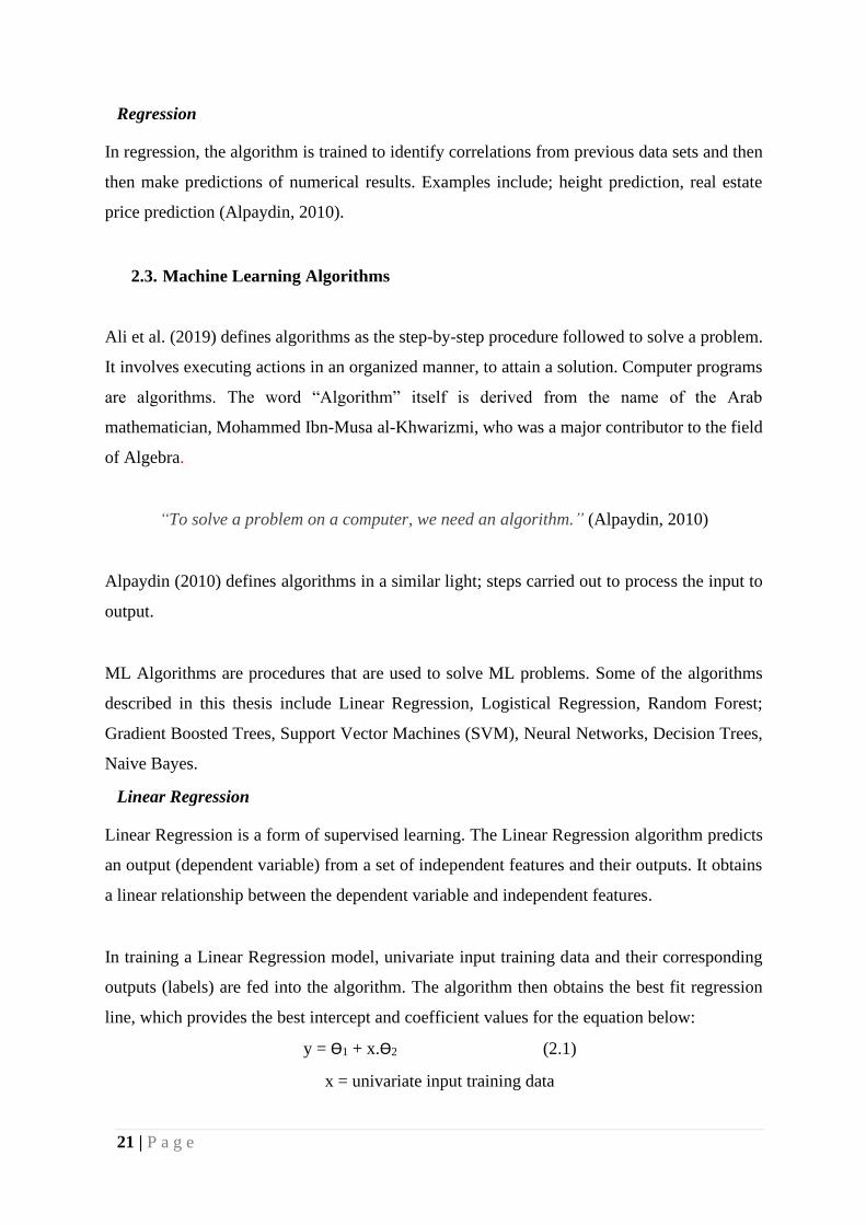
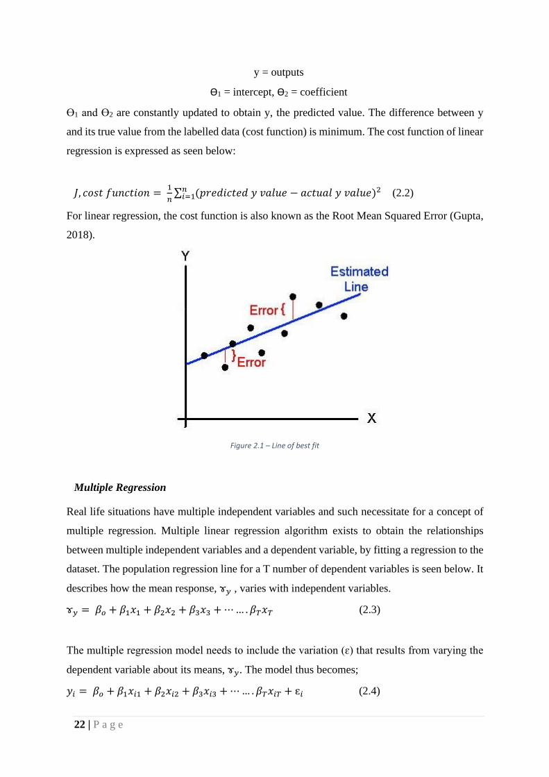
Ɵ1 and Ɵ2 are constantly updated to obtain y, the predicted value. The difference between y

and its true value from the labelled data (cost function) is minimum. The cost function of linear

regression is expressed as seen below:

𝐽, 𝑐𝑜𝑠𝑡 𝑓𝑢𝑛𝑐𝑡𝑖𝑜𝑛 = 1

𝑛∑ (𝑝𝑟𝑒𝑑𝑖𝑐𝑡𝑒𝑑 𝑦 𝑣𝑎𝑙𝑢𝑒 − 𝑎𝑐𝑡𝑢𝑎𝑙 𝑦 𝑣𝑎𝑙𝑢𝑒)2𝑛

𝑖=1 (2.2)

For linear regression, the cost function is also known as the Root Mean Squared Error (Gupta,

2018).

Figure 2.1 – Line of best fit

Multiple Regression

Real life situations have multiple independent variables and such necessitate for a concept of

multiple regression. Multiple linear regression algorithm exists to obtain the relationships

between multiple independent variables and a dependent variable, by fitting a regression to the

dataset. The population regression line for a T number of dependent variables is seen below. It

describes how the mean response, ɤ𝑦 , varies with independent variables.

ɤ𝑦 = 𝛽𝑜 + 𝛽1𝑥1 + 𝛽2𝑥2 + 𝛽3𝑥3 + ⋯ … . 𝛽𝑇𝑥𝑇 (2.3)

The multiple regression model needs to include the variation (ɛ) that results from varying the

dependent variable about its means, ɤ𝑦. The model thus becomes;

𝑦𝑖 = 𝛽𝑜 + 𝛽1𝑥𝑖1 + 𝛽2𝑥𝑖2 + 𝛽3𝑥𝑖3 + ⋯ … . 𝛽𝑇𝑥𝑖𝑇 + ɛ𝑖 (2.4)

23 | P a g e

A similar concept of minimizing the error, as in simple linear regression, is then employed

(Yale University, 1998).

Naïve Bayes Classifier

This is an algorithm that is based on the Bayes Theorem. It assumes independence amongst the

features of a dataset. The presence of a feature has no effect on the presence of another feature;

although both contribute towards the result.

The common use of the Naïve Bayes Classifier include; text classification, sentiment analysis,

face recognition, weather forecast, text and news classification, google search classification,

email spam filtering (Wasserman, 2004).

The Bayes Theorem is described mathematically as;

𝑃(𝐴|𝐵) = 𝑃(𝐵|𝐴)×𝑃(𝐴)

𝑃(𝐵) (2.5)

𝑃(𝐴|𝐵) is the probability of event A occurring, given event B has happened. Some underlying

concepts of the Bayes theorem according to Wasserman (2004) are;

• Probability of an event occurring stems from a belief and is not limited by frequency of

occurrence of an event. Therefore, an infinite number of events could be described via

probability. The probability of a flow being annular at some point, is determined by the

belief that it could be true; not by how many times it has occurred.

• Although fixed, parameters / attributes / features, could also be described using

probabilistic statements.

• From a probability distribution, point and interval estimates can be extracted.

In carrying out interference via the utilization of the Bayesian concept, a probability density

of a desired attribute is first chosen. This is called the prior distribution. A model that

describes the parameter, given the occurrence of another parameter is then chosen. The initial

prior distribution is then updated, after other parameters have also been observed. The

Bayesian concept thus has a strength of being relevant, with prior information, but its

subjective notion of probabilities slightly weakens it (Wasserman, 2004).

24 | P a g e

Advantages

• It is relatively easy to implement and has high performance when used for multi-class

prediction.

• In comparison to other classification algorithms, it requires lesser training data.

• It also performs highly according to Wasserman (2004) when categorical input

variables are compared to numerical variables.

Disadvantages

• Underlying assumption of independency amongst parameters or features (Wasserman,

2004).

Support Vector Machine (SVM)

The SVM is a supervised machine learning algorithm that is used for classification. Subsequent

to providing the SVM model with training data, it is able to appropriately categorise the data

as appropriate. It was developed in 1992 by Vapnik and has gained traction in modern machine

learning, due its high classification performance on moderately sized datasets. The computation

of a SVM becomes inefficient, when provided with large training examples.

An SVM, when provided with an appropriately sized dataset, develops a hyperplane that

separates the dataset. The hyperplane is a line that optimally separates data points and is also

popularly referred to as; the decision boundary. An optimal hyperplane minimises the margins

from the different categories. Scattered data points could be linearly inseparable; a new

dimension is added, creating a three-dimensional space. The prior mentioned concept could get

completed, thus the introduction of “kernels”. The SVM avoids employing the actual vectors

but uses the dot products between them, ensuring efficient computations. This concept

according, to Marsland (2015), is also used with other classifiers.

Decision Tree

The Decision tree algorithm is known to uniquely solve regression and classification problems.

The basic concept entails an algorithm that predicts a continuous or discrete class or value via

learning from decision rules, extracted from training data. Decision trees have been thus

grouped into; Categorical Variable Decision Tree and Continuous Variable Decision Tree. The

earlier mentioned system of classification is based on the goal or target of prediction. A

categorical variable decision tree aims to predict a categorical variable (Yes or No, Annular

25 | P a g e

Flow or Slug Flow etc.), while the continuous variable decision tree aims to predict a

continuous variable (Chauchan, 2020).

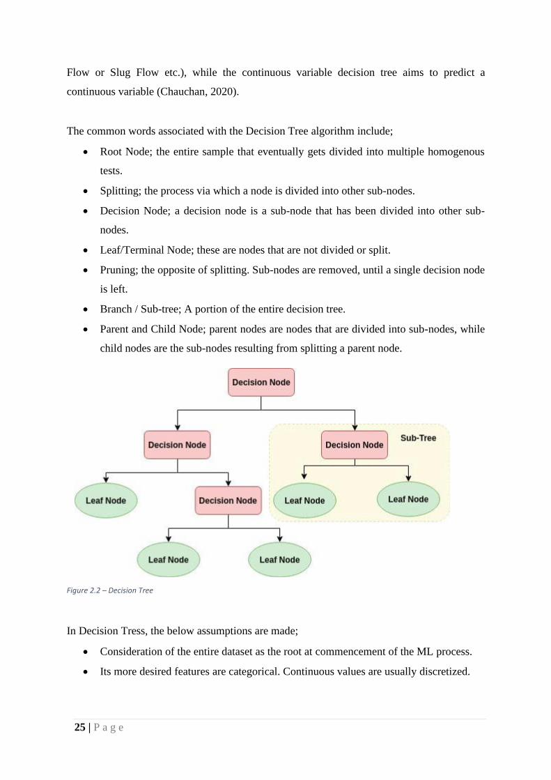
The common words associated with the Decision Tree algorithm include;

• Root Node; the entire sample that eventually gets divided into multiple homogenous

tests.

• Splitting; the process via which a node is divided into other sub-nodes.

• Decision Node; a decision node is a sub-node that has been divided into other sub-

nodes.

• Leaf/Terminal Node; these are nodes that are not divided or split.

• Pruning; the opposite of splitting. Sub-nodes are removed, until a single decision node

is left.

• Branch / Sub-tree; A portion of the entire decision tree.

• Parent and Child Node; parent nodes are nodes that are divided into sub-nodes, while

child nodes are the sub-nodes resulting from splitting a parent node.

Figure 2.2 – Decision Tree

In Decision Tress, the below assumptions are made;

• Consideration of the entire dataset as the root at commencement of the ML process.

• Its more desired features are categorical. Continuous values are usually discretized.

26 | P a g e

• Statistical approaches are the mechanisms via which features or attributes are placed as

root or internal nodes of the decision tree.

• Recursion is imperative for the distribution of records.

Decision Trees utilise the Sum of Product (SOP) representation, also known as Disjunctive

Normal Form. At a leaf node, all branches of the same class are a product of values. A sum

results when different branches end in that class (Chauchan, 2020).

Attributes selection is the process via which the appropriate features or attributes are selected

as root nodes, at each level. Several measures exist to facilitate such a process. Multiple

algorithms exist, that are used to develop sub-nodes. As more child nodes are created, the

homogeneity of resulting child nodes increase. The decision trees selects the split of nodes that

creates the most homogeneous child nodes. Beyond the need for homogeneity, algorithms are

also selected according to the type of target variables. An example is the ID3 algorithm

(Chauchan 2020).

ID3 algorithm

The ID3 algorithm develops a decision tree, via a one-way top-down search approach. It takes

the best decision at that point in time, without extensive consideration of past decisions. It

commences with the development of a root node, which is the original set. It then iterates

through each feature of the set, calculating entropy and information gain of the feature. The

feature with the highest information gain or lowest entropy is selected. The original set is then

split, to produce subsets via the feature selected in the first step. Recursion is then used by the

algorithm on each subset, not taking into consideration previously selected features (Chauchan,

2020).

Attribute Selection

Selecting an attribute is a complicated process. Researchers have recommended the certain

criteria discussed.

27 | P a g e

• Entropy

Entropy refers to the degree of randomness within data. The ease of analysis of data increases

with decreasing entropy. The ID3 algorithm operates based on the entropy notion; a branch

having an entropy of zero is considered as the “leaf node” and splits branches with entropies

of more than zero (Chauchan, 2020).

𝐸(𝑆) = ∑ −𝑐𝑖=1 𝑝𝑖𝑙𝑜𝑔2𝑝𝑖 (2.6)

S = current state

pi = Probability of an event i of state S or Percentage of class i in a node of state S.

For multiple features,

𝐸(𝑇, 𝑋) = ∑ 𝑃(𝑐)𝐸(𝑐)𝑐𝜖𝑋 (2.7)

• Information Gain

The Information Gain is a statistical tool used to measure how effective a specific feature splits

the training examples, based on the goal. Information gain according, to Chauchan (2020)

corresponds to a reduction in entropy. The ID3 algorithm also uses Information gain.

Mathematically,

𝐼𝐺 = E (Before splitting) + ∑ 𝐸(𝑗, 𝑎𝑓𝑡𝑒𝑟)𝑘𝑗=1 (2.8)

• Gini Index

The Gini Index is a cost function utilised for evaluation of a dataset after it has been split.

𝐺𝑖𝑛𝑖 = 1 − ∑ (𝑝𝑖)2𝑐

𝑖=1 (2.9)

From the mathematic function above, the Gini function will be biased towards classes with

higher probabilities. Homogeneity is directly proportional to the Gini Index.

The Gini function is the primary tool utilised by another Decision Tree algorithm, CART

(Classification and Regression Tree), in splitting nodes (Chauchan 2020).

• Gain Ratio

The Gain Ratio is an advancement over Information gain. It corrects for its tendency to be

biased towards features having distinctly large values. It considers the branches that would

result from splitting, before splitting (Chauchan, 2020).

28 | P a g e

𝐺𝑅 =𝐼𝐺

𝑆𝑝𝑙𝑖𝑡 𝑖𝑛𝑓𝑜𝑟𝑚𝑎𝑡𝑖𝑜𝑛 =

E (Before splitting)−∑ 𝐸(𝑗,𝑎𝑓𝑡𝑒𝑟)𝑘𝑗=1

∑ 𝑤𝑖(𝑙𝑜𝑔2𝑤𝑖)𝑘

𝑗=1

(2.10)

• Variance Reduction

Reduction in variance algorithm is usually used for regression. The best split of a dataset is

chosen, by reducing the variance to minimum (Chauchan, 2020).

𝑉𝑎𝑟𝑖𝑎𝑛𝑐𝑒 =∑(𝑋−𝑋)̅̅̅̅ 2

𝑛 (2.11)

• Chi-square

CHAID is the abbreviation for Chi-squared Automatic Interaction Detector. It represents the

statistical significance between the differences in the parent node and child node. The

significance is equal to the sum of squares of the differences between the actual target features

and forecasted. This is usually applied for categorisation problems (Chauchan, 2020).

Mathematically,

ɤ2 =∑(𝑂−𝐸)2

𝐸 (2.12)

A common problem with Decision Tress is over fitting. This results in inaccuracies when

attempting to predict from unknown datasets, not originally part of the training dataset.

Solutions include; Pruning and utilization of an advanced algorithm called “Random Forest”

(Chauchan, 2020).

Random Forest

The Random Forest is an algorithm that could be used for both regression and classification,

although it is mostly used for classification. Bremian is reported to have created this algorithm.

The Random Forest algorithm creates multiple decision trees from a dataset, then makes a

prediction based on the most responses provided by the decision trees. As earlier stated, it

solves the problem of over-fitting in decision trees. Another accurate definition of random

forest is; a classifier “consisting of a collection of decision trees, where each tree is constructed

by applying an algorithm A on the training set S and an additional random vector where the

29 | P a g e

vector is sampled from some distribution”. The prediction of the random forest is obtained by

a majority vote over the predictions of the individual trees.

The motivation for such a concept is that a decision tree would create good predictions, but

multiple decision trees would create better. If one decision tree produces errors in prediction,

the predictions of other decision trees would eventually eliminate the error of that tree. The

name “Random” results from the random nature in which trees are built and the randomness of

subsets when nodes are split. The randomness with which trees are created, sparks the

continuous interest in this algorithm. There exist two methods via which the randomness is

ensured: Bagging (also known as Bootstrap Aggregation) and Random feature selection (Yiu,

2019).

• Bagging

This is the process where every individual decision tree would develop trees based on random

sampling from the original dataset while, on the other hand, also taking replacements. The

original dataset does not break up into smaller subsets, and each tree is developed from each

sub-set. All decision trees created, on the contrary, are fed, according to Yiu (2019), a training

sample from the original dataset with a replacement.

• Random Feature Selection

Different decision trees by this method are created from an original dataset after randomly

testing its sub-features; this thus results in increased diversity between decision trees. There is

an increase in randomness via this method, as the trees can only select from the subsets. It is

also quicker, as there are lesser attributes to iterate over (Yiu 2019). Both earlier mentioned

methods intend to minimize variance, while also evading overfitting. Furthermore, shortening

is circumvented. More trees can be formed till the decrease in prediction error is minimal (Yiu,

2019).

Deep Learning (DL)

Deep Learning is perhaps the most stimulating branch of Machine Learning. It is implemented

in numerous technologies, like self-driving cars, software translators. Via DL, extreme

accuracy in predictions is possible. Several Deep Learning models include; Artificial Neural

30 | P a g e

Networks, Convolutional Neural Networks, Recurrent Neural Networks (RNN), Deep

Boltzmann machines, Auto Encoders.

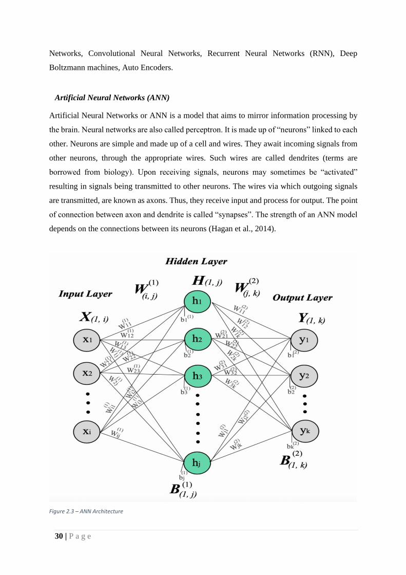
Artificial Neural Networks (ANN)

Artificial Neural Networks or ANN is a model that aims to mirror information processing by

the brain. Neural networks are also called perceptron. It is made up of “neurons” linked to each

other. Neurons are simple and made up of a cell and wires. They await incoming signals from

other neurons, through the appropriate wires. Such wires are called dendrites (terms are

borrowed from biology). Upon receiving signals, neurons may sometimes be “activated”

resulting in signals being transmitted to other neurons. The wires via which outgoing signals

are transmitted, are known as axons. Thus, they receive input and process for output. The point

of connection between axon and dendrite is called “synapses”. The strength of an ANN model

depends on the connections between its neurons (Hagan et al., 2014).

Figure 2.3 – ANN Architecture

31 | P a g e

Activation Function

The Activation Function of a neuron determines if the neuron will be “fired” or not. In detailed

terms; if the neuron would pass on a signal. This occurs via a calculation of the weighted sum

and adding some bias to the result. The bias is added, to introduce non-linearity into the signal

that is transmitted. Without the bias, a linear function would result from the neuron and would

not be able to model complex data. Rather, the one-dimensionality would restrict it to simple

or easy data (Izaugarat, 2018).

• Threshold activation function

For this type of activation function, a decision on transmitting a signal is dependent on a certain

threshold. If the input signal is above the threshold, the neuron is “fired” and outputs the exact

signal to the next layer (Luhaniwal, 2019).

• Sigmoid Activation function

The Sigmoid Activation function is a mathematical function used for problems that require its

solutions, in forms of probabilities. The Sigmoid function itself is S-shaped, having a maximum

of 1 and minimum of 0 (Luhaniwal, 2019).

• Hyperbolic Tangent function

The Hyperbolic Tangent function is also a mathematical function like the sigmoid function but

ranges from 1 to -1 (Luhaniwal, 2019).

• Rectified Linear Units

This is the most efficient activation function, ranging from 0 to infinity. This function is only

applied to hidden layers, while outputs could utilize other functions (Luhaniwal, 2019).

Methods of Adjusting Weights

• Brute-force Method

It is optimal when used in a single-layer feed-forward network. The optimal weight is selected,

after elimination of all other weights; the most minimal weight (the weight situated at the

32 | P a g e

bottom of the curve) is the optimal weight. This method is easily affected by Dimensionality

(Mayo, 2017).

• Batch-Gradient Descent

The Batch-Gradient Descent is a first-order algorithm that iterates through the data using

various angles of the function line. For a negative slope, it goes down the curve and for a

positive slope, it goes upwards. It is only effective, for a convex-shaped curve (Mayo, 2017).

• Stochastic Gradient Descent

For non-convex shaped curves, the Stochastic Gradient is used instead. Rather than iterating

through the entire data as in the Batch-gradient Descent, a portion of the original sample is

selected based on random probability. It is faster than the Batch-Gradient Descent (Mayo,

2017).

33 | P a g e

CHAPTER THREE

REVIEW OF FLOW ASSURANCE LITERATURE

This research work focuses on the “Multiphase Flow” aspect of Flow Assurance.

3.1. Definition of Multiphase Flow

There exist various definitions across literature, albeit similar. Michaelides et al. (2017) defined

multiphase flow as the simultaneous flow of more than one fluid phase through porous media.

Karen Tay defines multiphase flow as the simultaneous flow of materials with very distinct

velocity fields in each phase (Tay, 2017).

An analysis of the various definitions from existing literature insinuates the constant presence

of terminologies like “distinct phases”, “simultaneous flow”. In this thesis, multiphase flow is

simply defined as flow consisting of different phases. Such a scenario would intuitively be

difficult to predict or model, due to the different characteristics of various phases. Moreover,

occurrences below the surface have always been characterised by a huge degree of uncertainty.

An example is a flow consisting of gas, crude oil (liquid), water (liquid) and sand particles

(solid); it thus becomes important to understand the various characteristics of the phases, at

various operating conditions. The solid phase is usually transported by other phases of the

flow, in form of lumps and particles. Its flow is thus dependent on the size of the solids and the

motion of other phases. The liquid phase could either be a continuous or discontinuous phase,

depending on velocity. As a continuous phase, other elements are dispersed in it. The liquid is

suspended in other phases, if it’s the discontinuous phase. The gas phase is also similar to the

liquid phase, with the distinct difference being the high compressibility of gas (Sun, 2017).

3.2. Important Concepts in Multiphase Flow

Superficial Velocity

Superficial Velocity of a fluid is defined as the volumetric flow rate of the fluid divided by the

cross-sectional area in which the fluid is contained. The term “superficial” is similar to

34 | P a g e

“hypothetical”; it assumes the fluid being described is the only fluid in discussion. This term

was invented due to the difficulty in calculating velocities of multiphase flows across different

points. Superficial velocity is simpler to calculate and assumed to be constant over a distance

(Sun, 2017).

Liquid Holdup

Geocities (2015) defined liquid holdup as the percentage or fraction of a pipe occupied by the

liquid phase, at the same instant. Liquid holdup is an essential calculation, due to it being

required for other calculations; heat transfer, mixture density, effective viscosity. The value

thus ranges from 0% or 0 (in single-phase gas flows) to 100% or 1 (in single-phase liquid

flows). Liquid holdup is measured via several experimental methods; resistivity probes,

capacitance probes, trapping a segment of the flow stream between quick closing valves and

measuring the volume of liquid trapped (Geocities, 2015).

“Void fraction” is a term that is used instead of “Liquid Holdup”, usually. It represents the

fraction of pipe occupied by gas. It is thus the “Liquid Holdup” subtracted from 1.

Geocities (2015) further explicitly states that liquid holdup cannot be determined analytically.

Liquid holdup is a function of the following variables; flow pattern / regime, pipe

characteristics (roughness, diameter), fluid properties (gas & liquid).

Flow Patterns

Flow patterns refer to the geometric distribution of individual phases in a multiphase flow.

Various flow patterns have been identified via different methods, visual inspection, advanced

technologies. The differences in the geometric distributions of the individual phases result in

differences in properties like velocity, void fraction, holdup. Numerous attempts have been

made to classify the different flow patterns.

The determination of flow patterns in the Oil and Gas Industry is of utmost importance. Flow

patterns are used to determine the pressure drops for flows from the reservoir through the

wellbore, to the surface and beyond. Numerous efforts have thus been made to identify such

patterns (Azzopardi, 2010).

35 | P a g e

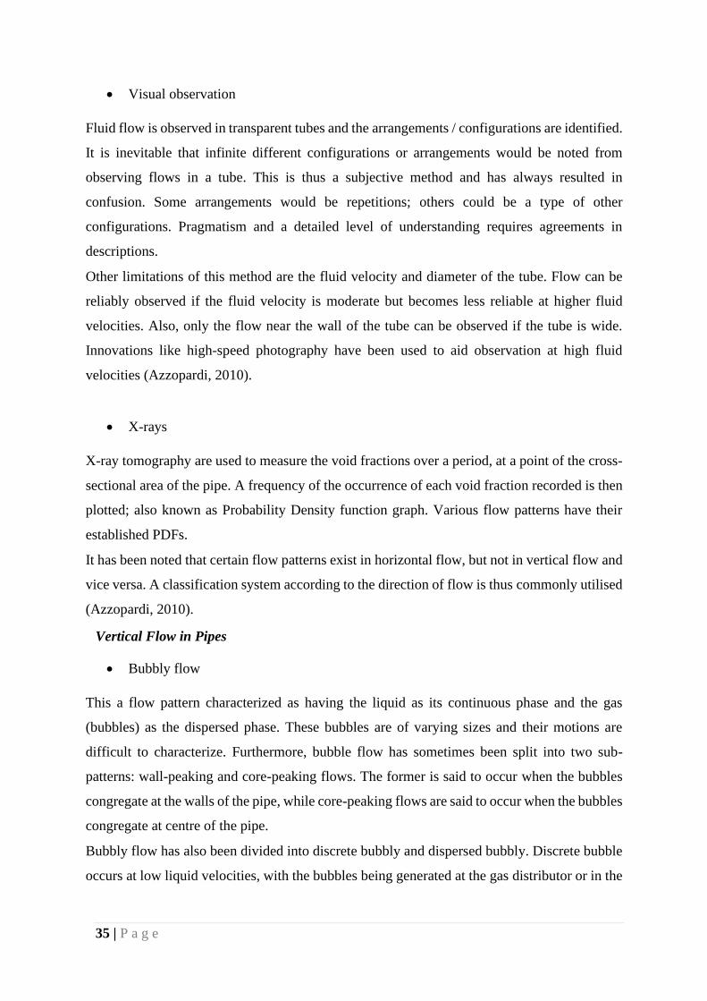
• Visual observation

Fluid flow is observed in transparent tubes and the arrangements / configurations are identified.

It is inevitable that infinite different configurations or arrangements would be noted from

observing flows in a tube. This is thus a subjective method and has always resulted in

confusion. Some arrangements would be repetitions; others could be a type of other

configurations. Pragmatism and a detailed level of understanding requires agreements in

descriptions.

Other limitations of this method are the fluid velocity and diameter of the tube. Flow can be

reliably observed if the fluid velocity is moderate but becomes less reliable at higher fluid

velocities. Also, only the flow near the wall of the tube can be observed if the tube is wide.

Innovations like high-speed photography have been used to aid observation at high fluid

velocities (Azzopardi, 2010).

• X-rays

X-ray tomography are used to measure the void fractions over a period, at a point of the cross-

sectional area of the pipe. A frequency of the occurrence of each void fraction recorded is then

plotted; also known as Probability Density function graph. Various flow patterns have their

established PDFs.

It has been noted that certain flow patterns exist in horizontal flow, but not in vertical flow and

vice versa. A classification system according to the direction of flow is thus commonly utilised

(Azzopardi, 2010).

Vertical Flow in Pipes

• Bubbly flow

This a flow pattern characterized as having the liquid as its continuous phase and the gas

(bubbles) as the dispersed phase. These bubbles are of varying sizes and their motions are

difficult to characterize. Furthermore, bubble flow has sometimes been split into two sub-

patterns: wall-peaking and core-peaking flows. The former is said to occur when the bubbles

congregate at the walls of the pipe, while core-peaking flows are said to occur when the bubbles

congregate at centre of the pipe.

Bubbly flow has also been divided into discrete bubbly and dispersed bubbly. Discrete bubble

occurs at low liquid velocities, with the bubbles being generated at the gas distributor or in the

36 | P a g e

process of nucleate boiling. Dispersed bubbly occurs at high liquid velocities, with large

bubbles breaking down into smaller bubbles (Azzopardi, 2010).

• Plug flow

Plug glow is also known as slug flow. It occurs when bubbles coalescence and thus, result in

an increase in the size of the bubbles. The resulting bubbles are shaped like bullets. These

bubbles are called Taylor bubbles. The Taylor bubbles occupy most of the pipe and are

surrounded by films of liquids. Smaller bubbles are also located in the liquid slug between the

huge Taylor bubbles. Recent literature shows that plug flow is limited to relatively small

diameter pipes (< 150 mm), rather flow transitions from bubble to churn flow (Azzopardi,

2010).

• Churn flow

A churning flow pattern is noted at higher velocities. It is usually characterized by oscillatory

fluid motion resulting from breakdown of Taylor bubbles. It is sometimes referred to as semi-

annular flow when it occurs at higher gas velocities. Plug and churn flow patterns are often

collectively referred to as intermittent flow (Azzopardi, 2010).

• Annular flow

Azzopardi (2010) described annular flow as the flow pattern where liquid travels as a film on

the walls of the pipe. In some cases, the liquid also exists as drops in the central gas core. Such

a pattern is also referred to as mist flow. “Wispy annular flow” is also used in certain cases; at

high liquid flow rates, the concentration of liquid droplets in the central gas core is extremely

high resulting in tendrils of the liquid being evident.

Another description of annular flow is provided below.

Annular flow, also known as channel flow, is a type of multiphase flow that is said to occur in

a pipe when the lighter fluid occupies the centre of the pipe and the denser fluid flows occupies

the walls of the pipe as thin film. In the context of oil and gas, gas would be at the centre while

water or oil flows as a thin film over the walls of the pipe. In a scenario where flow core

37 | P a g e

contains entrained liquid droplets, the flow is usually referred to as “annular-dispersed” flow,

while it is called “pure annular” flow in the absence of entrained liquid droplets. Also, both

flows of the near-wall liquid film and gas core are characterized as concurrent and

countercurrent. The void fraction of annular flow has been known to be greater than 75-80%

(Azzopardi, 2010).

Horizontal Flow in Pipes

The flow patterns noted in vertical flows, in addition to stratified flow patterns, are the flow

patterns noted in horizontal flows.

• Stratified flow

In the Stratified flow pattern, the densities of the phases is at the bottom of the pipe; density of

the phases is the property that determines how the phases are configured. The stratified-flow

pattern is further divided into two sub-patterns; stratified-smooth and stratified-wavy.

Stratified-smooth is characterized by a gas-liquid interface that is smooth. It occurs at lower

gas rates than the stratified-wavy pattern. In the stratified-wavy flow pattern, the interface is

wavy due to the higher gas rates (Azzopardi, 2010).

• Intermittent flow

In horizontal flow, intermittent flow is made up of two categories: slug and elongated bubble

patterns. The elongated bubble pattern is known to contain large sized bubbles in the upper

zone of the liquid phase, while the slug flow pattern is characterized by having both large and

small bubbles of gas (Azzopardi, 2010).

Costigan and Whalley (1997) combined the PDF concept and segmented impedance electrodes

to establish six flow patterns: discrete bubble, spherical cap bubble, stable slug, unstable slug,

churn and annular flow. The descriptions of the flow patterns are stated below;

• The discrete flow is portrayed by a PDF having single peak at low void fraction.

• The spherical cap bubble is portrayed by a PDF that has a single peak at low void

fraction and then a tail that extends.

38 | P a g e

• The slug flow is portrayed by a PDF that has two peaks. One peak is at a low void

fraction and the other is at a higher void fraction.

• The churn flow is portrayed by a PDF that has a single peak at high void fraction and

then a tail that extends.

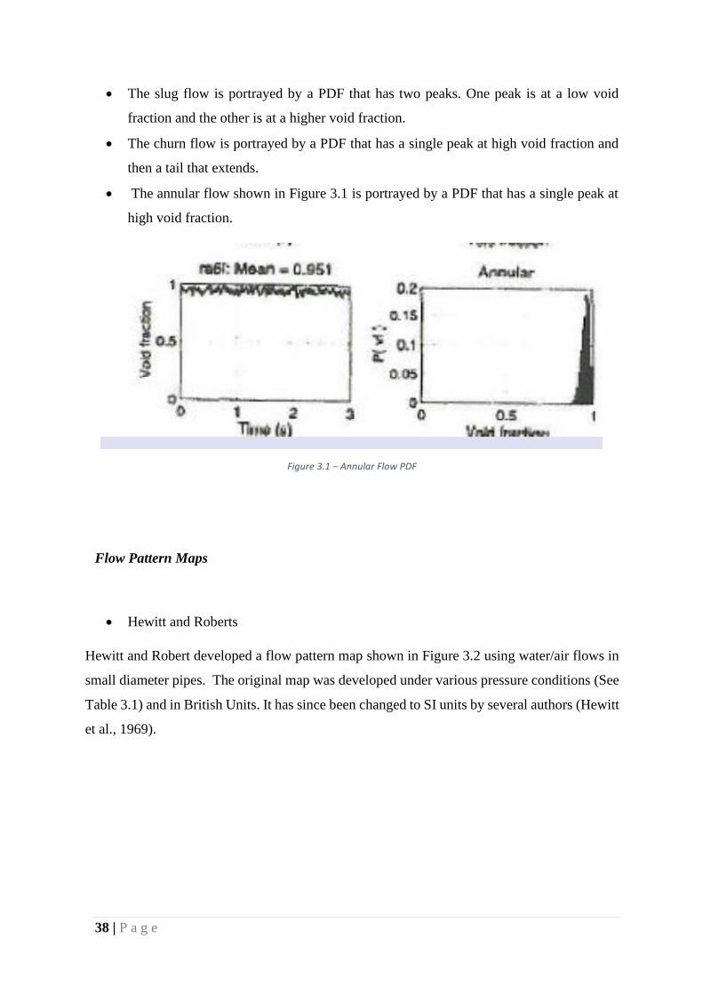
• The annular flow shown in Figure 3.1 is portrayed by a PDF that has a single peak at

high void fraction.

Figure 3.1 – Annular Flow PDF

Flow Pattern Maps

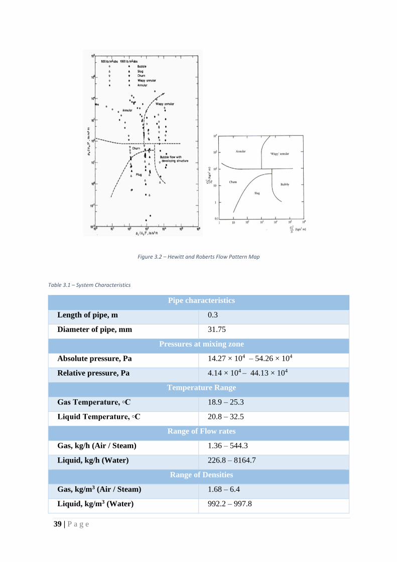
• Hewitt and Roberts

Hewitt and Robert developed a flow pattern map shown in Figure 3.2 using water/air flows in

small diameter pipes. The original map was developed under various pressure conditions (See

Table 3.1) and in British Units. It has since been changed to SI units by several authors (Hewitt

et al., 1969).

39 | P a g e

Figure 3.2 – Hewitt and Roberts Flow Pattern Map

Table 3.1 – System Characteristics

Pipe characteristics

Length of pipe, m 0.3

Diameter of pipe, mm 31.75

Pressures at mixing zone

Absolute pressure, Pa 14.27 × 104 – 54.26 × 104

Relative pressure, Pa 4.14 × 104 – 44.13 × 104

Temperature Range

Gas Temperature, ◦C 18.9 – 25.3

Liquid Temperature, ◦C 20.8 – 32.5

Range of Flow rates

Gas, kg/h (Air / Steam) 1.36 – 544.3

Liquid, kg/h (Water) 226.8 – 8164.7

Range of Densities

Gas, kg/m3 (Air / Steam) 1.68 – 6.4

Liquid, kg/m3 (Water) 992.2 – 997.8

40 | P a g e

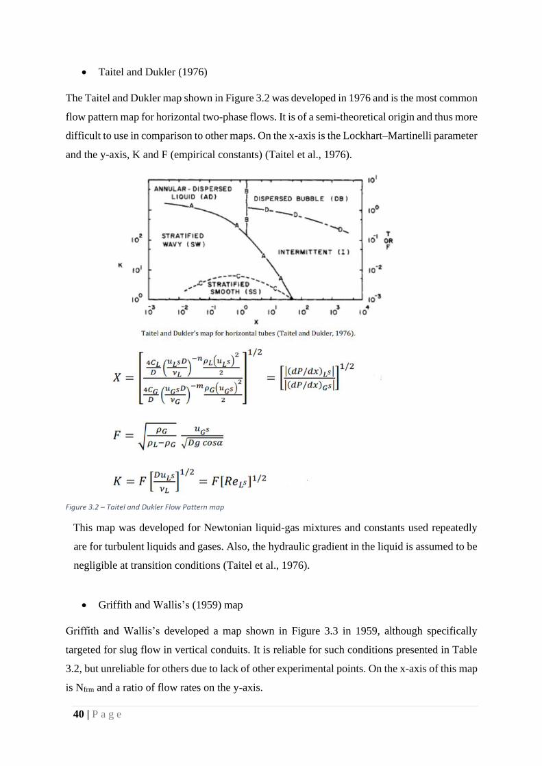
• Taitel and Dukler (1976)

The Taitel and Dukler map shown in Figure 3.2 was developed in 1976 and is the most common

flow pattern map for horizontal two-phase flows. It is of a semi-theoretical origin and thus more

difficult to use in comparison to other maps. On the x-axis is the Lockhart–Martinelli parameter

and the y-axis, K and F (empirical constants) (Taitel et al., 1976).

Figure 3.2 – Taitel and Dukler Flow Pattern map

This map was developed for Newtonian liquid-gas mixtures and constants used repeatedly

are for turbulent liquids and gases. Also, the hydraulic gradient in the liquid is assumed to be

negligible at transition conditions (Taitel et al., 1976).

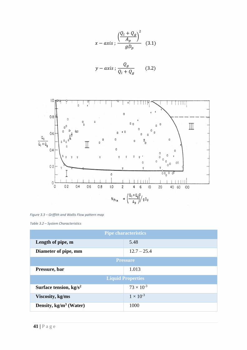
• Griffith and Wallis’s (1959) map

Griffith and Wallis’s developed a map shown in Figure 3.3 in 1959, although specifically

targeted for slug flow in vertical conduits. It is reliable for such conditions presented in Table

3.2, but unreliable for others due to lack of other experimental points. On the x-axis of this map

is Nfrm and a ratio of flow rates on the y-axis.

41 | P a g e

𝑥 − 𝑎𝑥𝑖𝑠 ;

(𝑄𝑙 + 𝑄𝑔

𝐴𝑝)

2

𝑔𝐷𝑝 (3.1)

𝑦 − 𝑎𝑥𝑖𝑠 ; 𝑄𝑔

𝑄𝑙 + 𝑄𝑔 (3.2)

Figure 3.3 – Griffith and Wallis Flow pattern map



Length of pipe, m 5.48

Diameter of pipe, mm 12.7 – 25.4

Pressure

Pressure, bar 1.013

Liquid Properties

Surface tension, kg/s2 73 × 10-3

Viscosity, kg/ms 1 × 10-3

Density, kg/m3 (Water) 1000

42 | P a g e

• Golan and Stenning’s (1969) map

Sequel to noting disagreements between maps of vertical flows, Golan and Stenning developed

two new maps shown in Figures 3.4 and 3.5 in 1969. The two maps were for vertical upward

and downward flows.

Figure 3.4 – Golan and Stenning’s Down-flow pattern map

43 | P a g e

Figure 3.5 - Golan and Stenning’s (1969) Up-flow pattern map



Length of pipe, m 3

Diameter of pipe, mm 38.1

Pressure

Pressure, bar 3.12

Liquid Properties

Surface tension, kg/s2 72 × 10-3

Viscosity, kg/ms 1 × 10-3

Density, kg/m3 (Water) 1000

Liquid Temperature, ◦C 20

Range of Flow rates

Gas, kg/h (Air) 10.77 – 3067.5

Liquid, kg/h (Water) 1000 - 10000

44 | P a g e

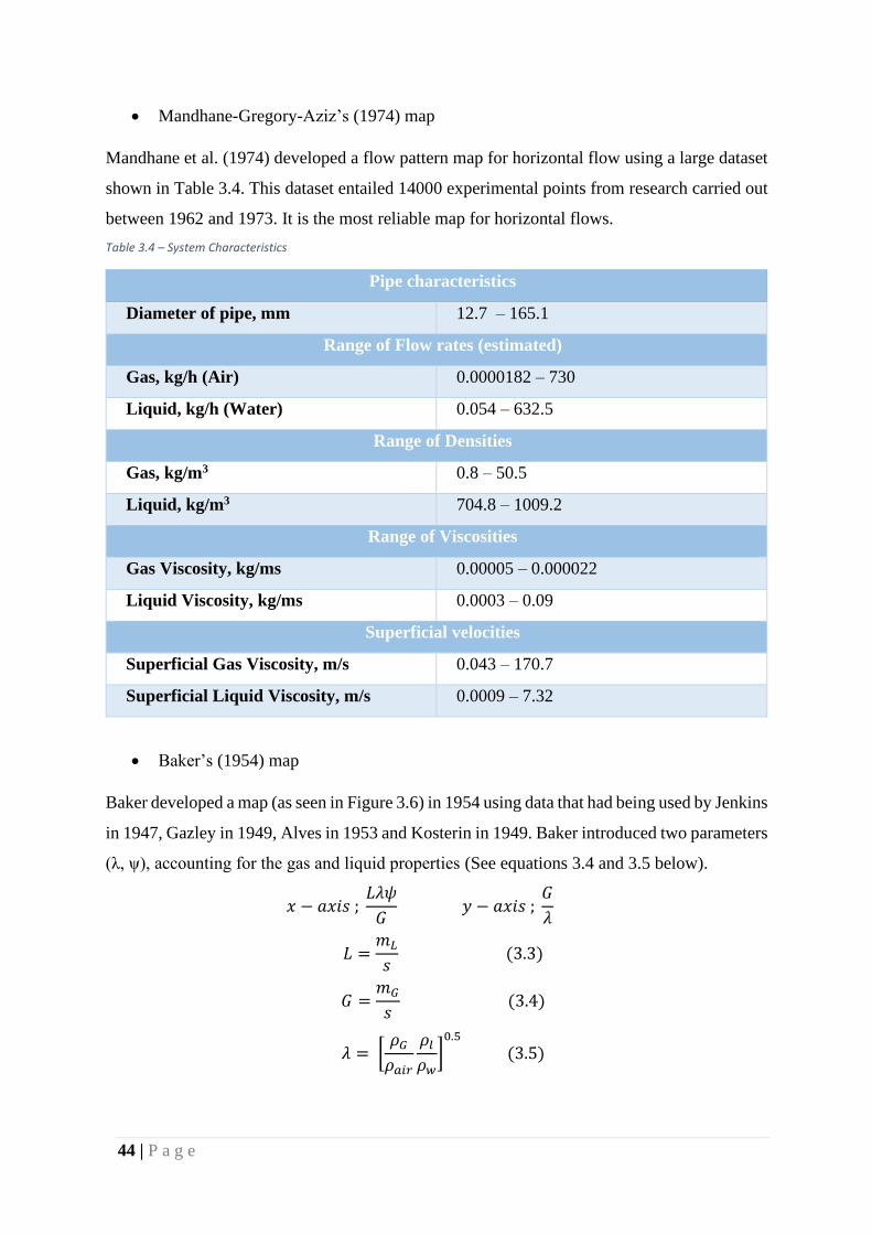
• Mandhane-Gregory-Aziz’s (1974) map

Mandhane et al. (1974) developed a flow pattern map for horizontal flow using a large dataset

shown in Table 3.4. This dataset entailed 14000 experimental points from research carried out

between 1962 and 1973. It is the most reliable map for horizontal flows.




Range of Flow rates (estimated)

Gas, kg/h (Air) 0.0000182 – 730

Liquid, kg/h (Water) 0.054 – 632.5

Range of Densities

Gas, kg/m3 0.8 – 50.5

Liquid, kg/m3 704.8 – 1009.2

Range of Viscosities

Gas Viscosity, kg/ms 0.00005 – 0.000022

Liquid Viscosity, kg/ms 0.0003 – 0.09

Superficial velocities

Superficial Gas Viscosity, m/s 0.043 – 170.7

Superficial Liquid Viscosity, m/s 0.0009 – 7.32

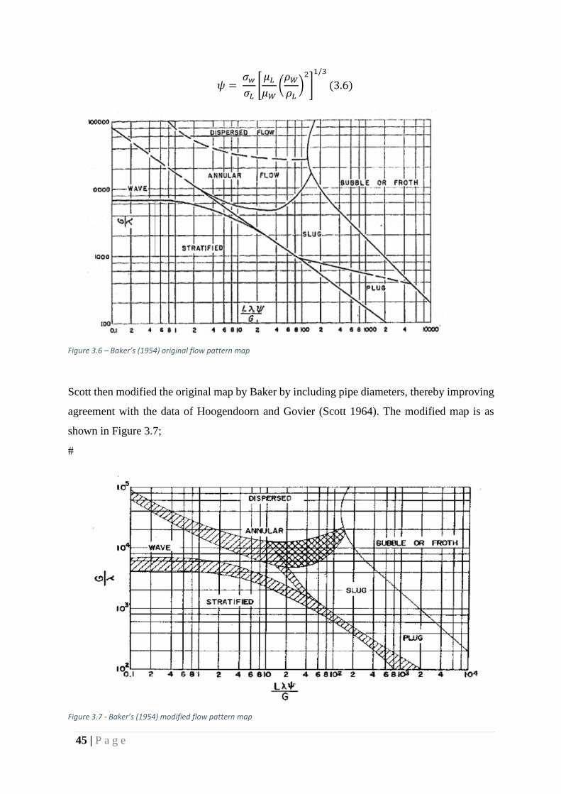
• Baker’s (1954) map

Baker developed a map (as seen in Figure 3.6) in 1954 using data that had being used by Jenkins

in 1947, Gazley in 1949, Alves in 1953 and Kosterin in 1949. Baker introduced two parameters

(λ, ψ), accounting for the gas and liquid properties (See equations 3.4 and 3.5 below).

𝑥 − 𝑎𝑥𝑖𝑠 ; 𝐿𝜆𝜓

𝐺 𝑦 − 𝑎𝑥𝑖𝑠 ;

𝐺

𝜆

𝐿 =𝑚𝐿

𝑠 (3.3)

𝐺 =𝑚𝐺

𝑠 (3.4)

𝜆 = [𝜌𝐺

𝜌𝑎𝑖𝑟

𝜌𝑙

𝜌𝑤]

0.5

(3.5)

45 | P a g e

𝜓 = 𝜎𝑤

𝜎𝐿[

𝜇𝐿

𝜇𝑊(

𝜌𝑊

𝜌𝐿)

2

]

1/3

(3.6)

Figure 3.6 – Baker’s (1954) original flow pattern map

Scott then modified the original map by Baker by including pipe diameters, thereby improving

agreement with the data of Hoogendoorn and Govier (Scott 1964). The modified map is as

shown in Figure 3.7;

#

Figure 3.7 - Baker’s (1954) modified flow pattern map

46 | P a g e

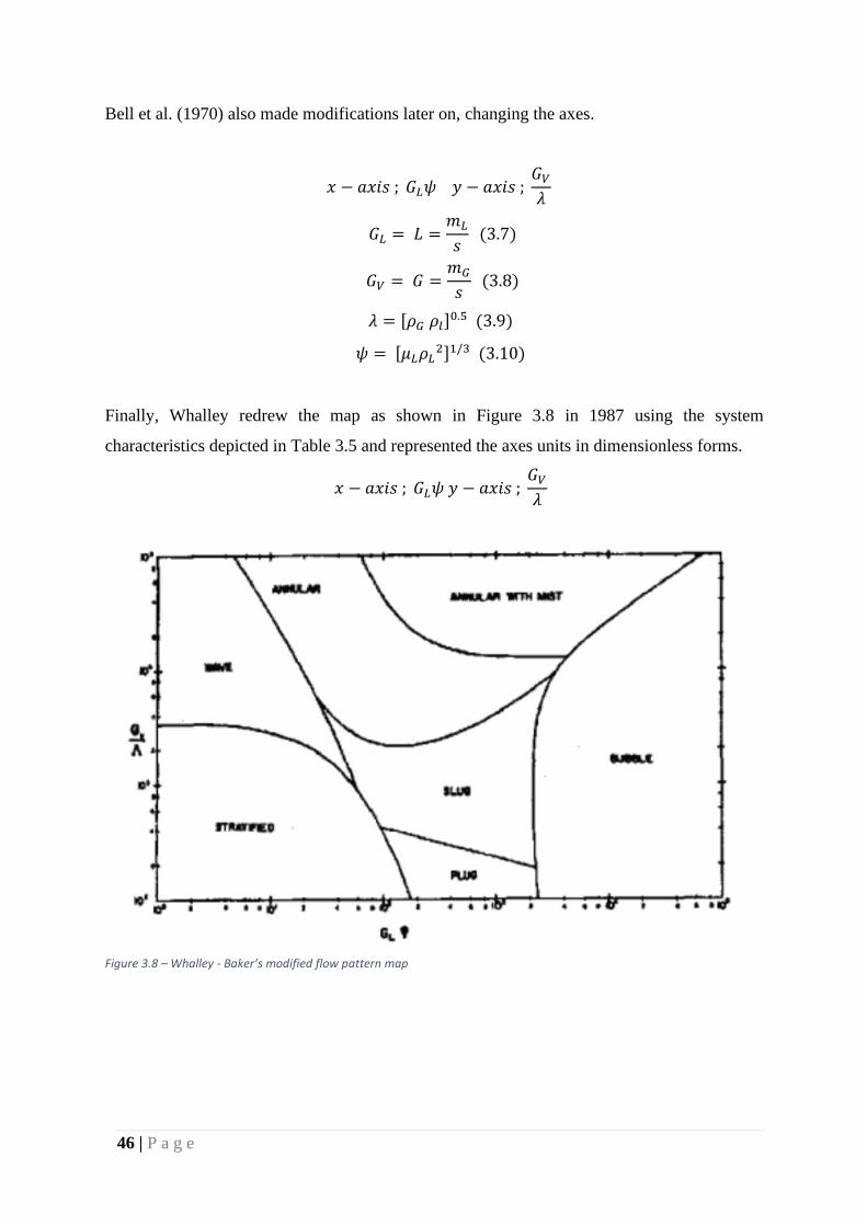
Bell et al. (1970) also made modifications later on, changing the axes.

𝑥 − 𝑎𝑥𝑖𝑠 ; 𝐺𝐿𝜓 𝑦 − 𝑎𝑥𝑖𝑠 ; 𝐺𝑉

𝜆

𝐺𝐿 = 𝐿 =𝑚𝐿

𝑠 (3.7)

𝐺𝑉 = 𝐺 =𝑚𝐺

𝑠 (3.8)

𝜆 = [𝜌𝐺 𝜌𝑙]0.5 (3.9)

𝜓 = [𝜇𝐿𝜌𝐿2]1/3 (3.10)

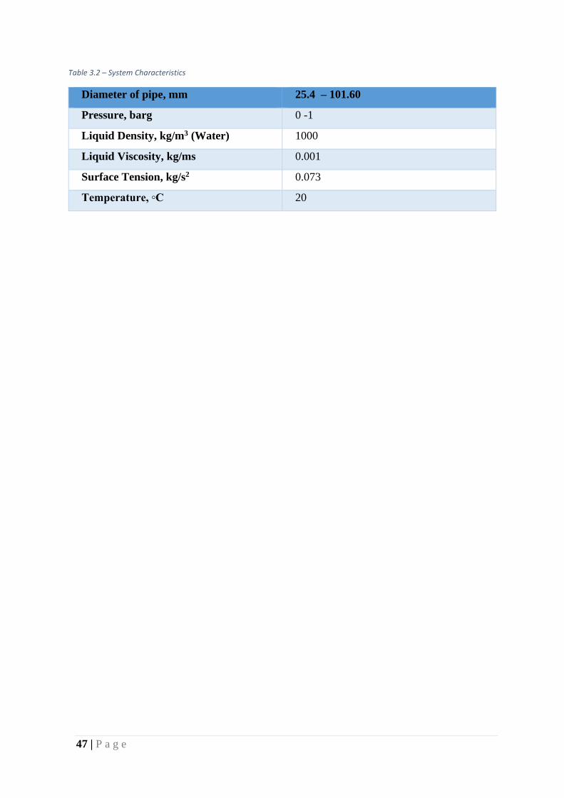
Finally, Whalley redrew the map as shown in Figure 3.8 in 1987 using the system

characteristics depicted in Table 3.5 and represented the axes units in dimensionless forms.

𝑥 − 𝑎𝑥𝑖𝑠 ; 𝐺𝐿𝜓 𝑦 − 𝑎𝑥𝑖𝑠 ; 𝐺𝑉

𝜆

Figure 3.8 – Whalley - Baker’s modified flow pattern map

47 | P a g e



Pressure, barg 0 -1

Liquid Density, kg/m3 (Water) 1000

Liquid Viscosity, kg/ms 0.001

Surface Tension, kg/s2 0.073

Temperature, ◦C 20

48 | P a g e

CHAPTER FOUR

METHODOLOGY

Literature review indicates the existence of different methodologies for prediction via Machine

Learning. The two most popular frameworks were defined by Guo (2017) and Chollet (2017).

4.1. Guo’s (2017) Method

1. Data collection

The relevant data for developing the predictive model is appropriately collected. Data is usually

represented in tables. It is important that the actual data is collected; else the predictive model

will be affected.

2. Data preparation

The data is then prepared for the training step. Preparation would include deleting duplicates,

treating rows / columns not having missing values, conversion of data types, rearranging data

to inculcate randomization. Such are necessary to ensure the data fed into the algorithm is not

biased. An extra test for bias in data is data visualization. Data visualization shows the existing

relationships between features. The final step involved in preparation is splitting the data into

training, testing and validation.

3. Selection of Model

The appropriate training algorithm is then selected. This would be based on the type of data

and expectations of the predictive model. Does the model aim to predict continuous or discrete

model? Is a time series data?

4. Model training

The portion of the dataset for training (training data) is then fed into the model. This could be

done via programming tools like Python, MATLAB.

49 | P a g e

5. Model Evaluation

A metric is used to measure the predictive efficiency of the developed model. Such a metric is

popularly the mean square error. Evaluation is carried out some part of the data that was not

fed into the algorithm (test dataset).

6. Parameter tuning

A few examples of model hyper parameters include the learning rate of the algorithm, original

guesses (initialization), number of neurons, number of layers. The aforementioned could be

adjusted to obtain better performance.

7. Final Predictions

The model is then used to make predictions on some part of the data that was not fed into the

algorithm (validation dataset) (Guo, 2017).

4.2. Chollet’s (2017) Method

1. Dataset assembly and problem definition

The aim of the predictive model is clearly defined. Subsequently, the relevant dataset is

assembled. Its constituents should be as accurate and precise, as needed.

2. Success definition

A successful predictive model should be defined. What is the degree of accuracy required by

the predictive models, such that predicted values are not off by a distance?

3. Evaluation protocol definition

The methodology required for the evaluation of the predictive model is also defined.

4. Data preparation

The dataset is prepared. Like Guo (2017), only relevant and clean data should be fed into the

training algorithm.

50 | P a g e

5. Model development

A model is then developed that fits the definition of what a successful predictive model is.

6. Improve developed model.

The already developed model is improved upon, to the extent that it over fits the dataset.

7. Parameter tuning

Model hyperparameters are then adjusted, until a model that can generalize effectively is

developed (Chollet, 2017).

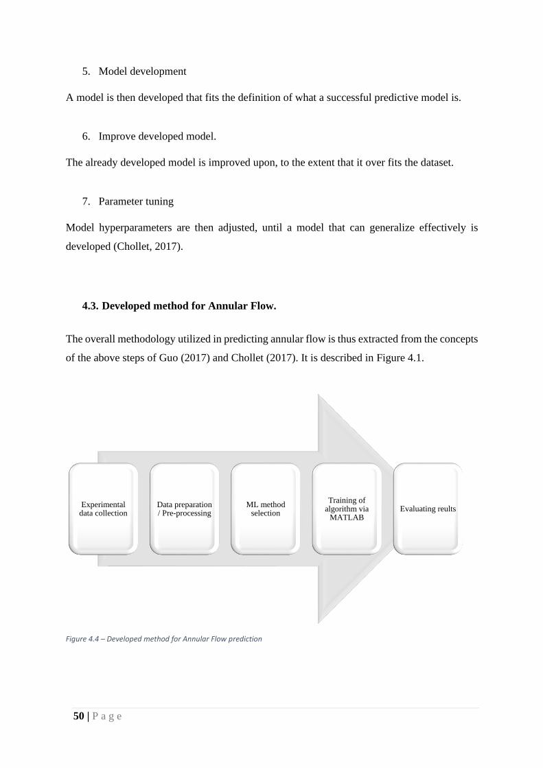
4.3. Developed method for Annular Flow.

The overall methodology utilized in predicting annular flow is thus extracted from the concepts

of the above steps of Guo (2017) and Chollet (2017). It is described in Figure 4.1.

Figure 4.4 – Developed method for Annular Flow prediction

Experimental data collection

Data preparation / Pre-processing

ML method selection

Training of algorithm via

MATLABEvaluating reults

51 | P a g e

1. Data collection

The liquid holdup over a period of 15,000 time points (0.001s to 15s) were recorded for an air

– water system. The system’s gas superficial velocity was varied (17 different gas superficial

velocities ranged from 6.17 ms-1 to 16.05 ms-1), while the liquid superficial velocity (0.02 ms-

1) was kept constant.

The experimental procedure from which the data is obtained is described below.

Compressed air was firstly used to pressurise the flow loop and then delivered to a mixer via

two ring pumps. The air mixes with water in the mixer; the water is pumped via a centrifugal

pimp from a two-phase separator.

The mixer is made up of a 105 mm diameter tube placed at the centre of the 127 mm internal

diameter test section. The pipe wall is covered by a water film, the pipe’s centre region is filled

with air. A calibrated vortex and turbine meter are used as air and water flow meters,

respectively.

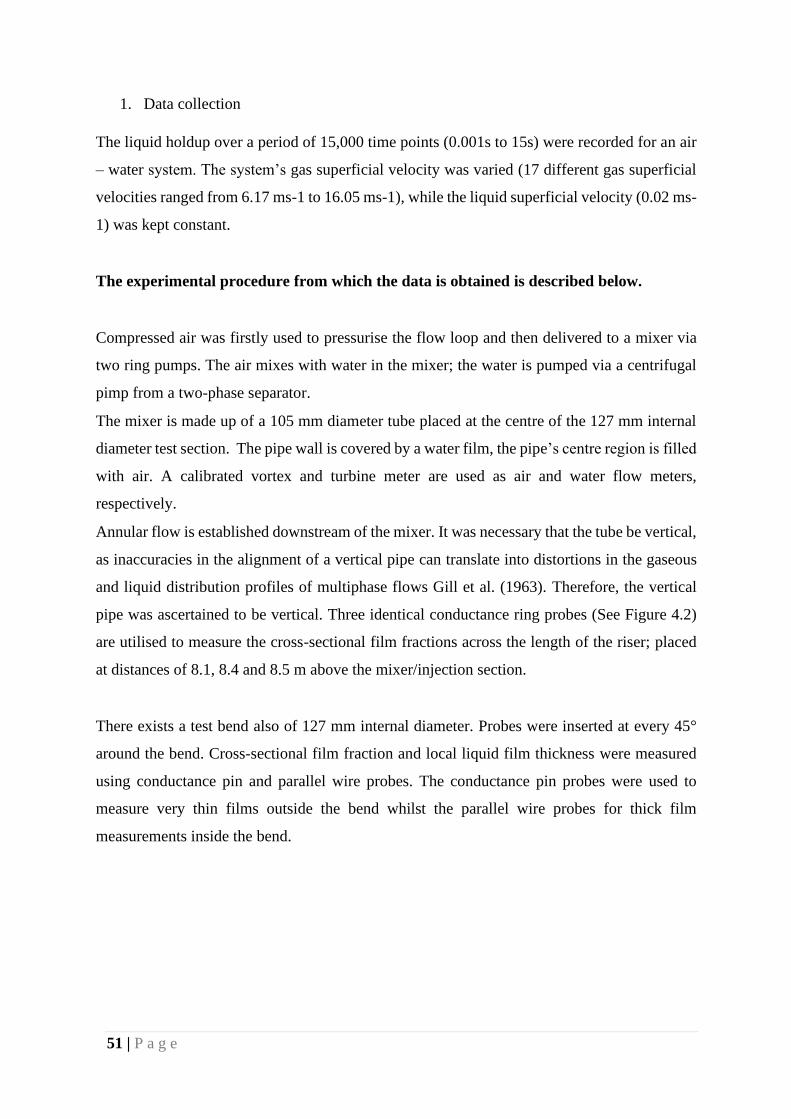
Annular flow is established downstream of the mixer. It was necessary that the tube be vertical,

as inaccuracies in the alignment of a vertical pipe can translate into distortions in the gaseous

and liquid distribution profiles of multiphase flows Gill et al. (1963). Therefore, the vertical

pipe was ascertained to be vertical. Three identical conductance ring probes (See Figure 4.2)

are utilised to measure the cross-sectional film fractions across the length of the riser; placed

at distances of 8.1, 8.4 and 8.5 m above the mixer/injection section.

There exists a test bend also of 127 mm internal diameter. Probes were inserted at every 45°

around the bend. Cross-sectional film fraction and local liquid film thickness were measured

using conductance pin and parallel wire probes. The conductance pin probes were used to

measure very thin films outside the bend whilst the parallel wire probes for thick film

measurements inside the bend.

52 | P a g e

Figure 4.2 – The locations of the measurement of film fraction on the transparent test section of the riser

2. Data preparation

The data was split into three excel workbooks, as there were three probes measuring the liquid

holdup across the system. There was thus three excel workbooks, titled; x = 8.1 m, x = 8.3 m,

x = 8.5 m (“x” represents the probe distance across the pipe). Each workbook contained 17 data

sheets, representing the 17 different gas superficial velocities contained in the original data.

Furthermore, each sheet contained the various liquid holdups and time points at which they

were measured.

53 | P a g e

3. ML method selection

The Artificial Neural Network (ANN) has been chosen as the desired method due to its ability

to predict nonlinear data and its renowned efficiency with time series. MATLAB has a Neural

Network toolbox for time series.

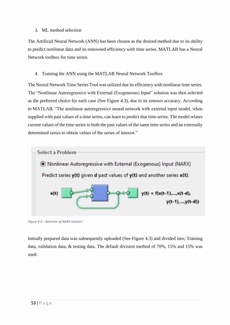
4. Training the ANN using the MATLAB Neural Network Toolbox

The Neural Network Time Series Tool was utilized due its efficiency with nonlinear time series.

The “Nonlinear Autoregressive with External (Exogeneous) Input” solution was then selected

as the preferred choice for each case (See Figure 4.3), due to its renown accuracy. According

to MATLAB, “The nonlinear autoregressive neural network with external input model, when

supplied with past values of a time series, can learn to predict that time series. The model relates

current values of the time series to both the past values of the same time series and an externally

determined series to obtain values of the series of interest.”

Figure 4.3 – Selection of NARX Solution

Initially prepared data was subsequently uploaded (See Figure 4.3) and divided into; Training

data, validation data, & testing data. The default division method of 70%, 15% and 15% was

used.

54 | P a g e

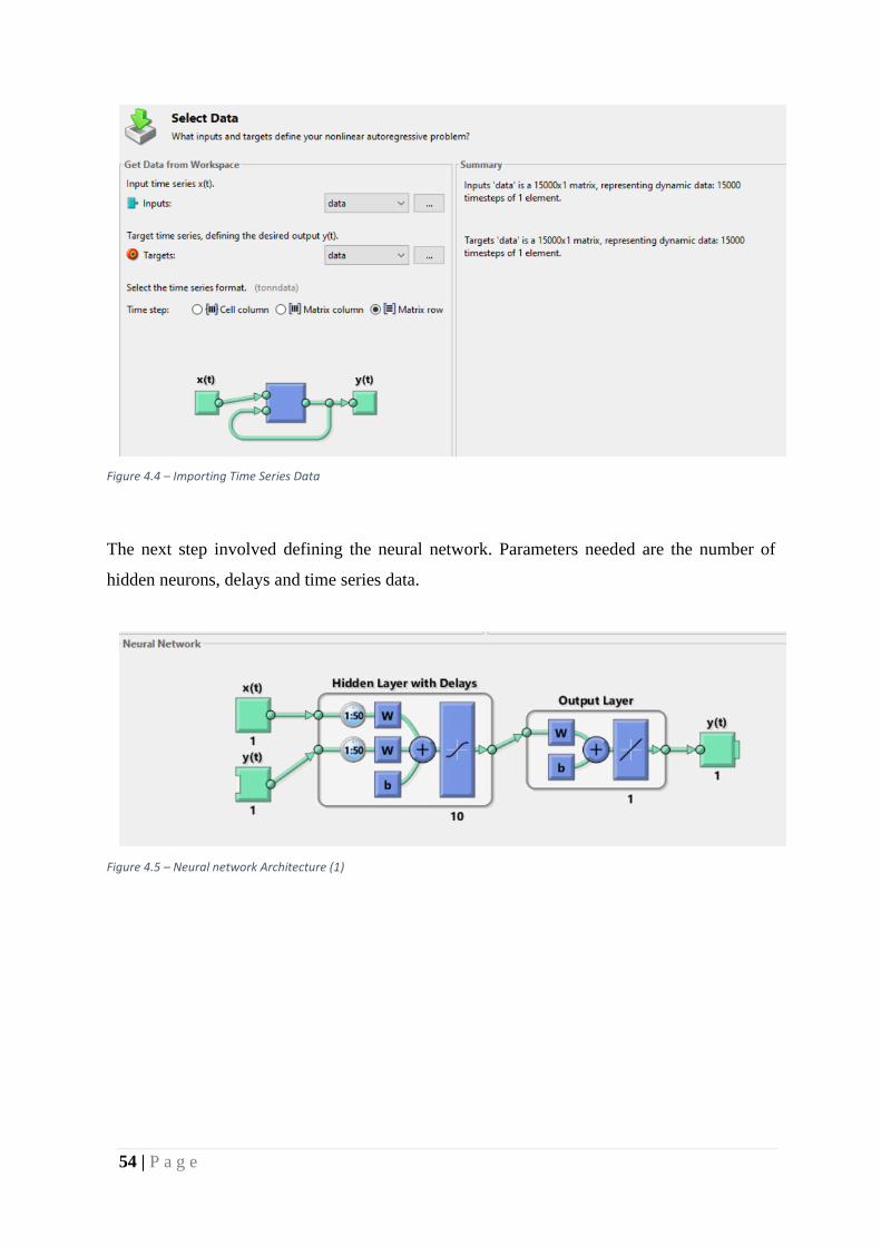
Figure 4.4 – Importing Time Series Data

The next step involved defining the neural network. Parameters needed are the number of

hidden neurons, delays and time series data.

Figure 4.5 – Neural network Architecture (1)

55 | P a g e

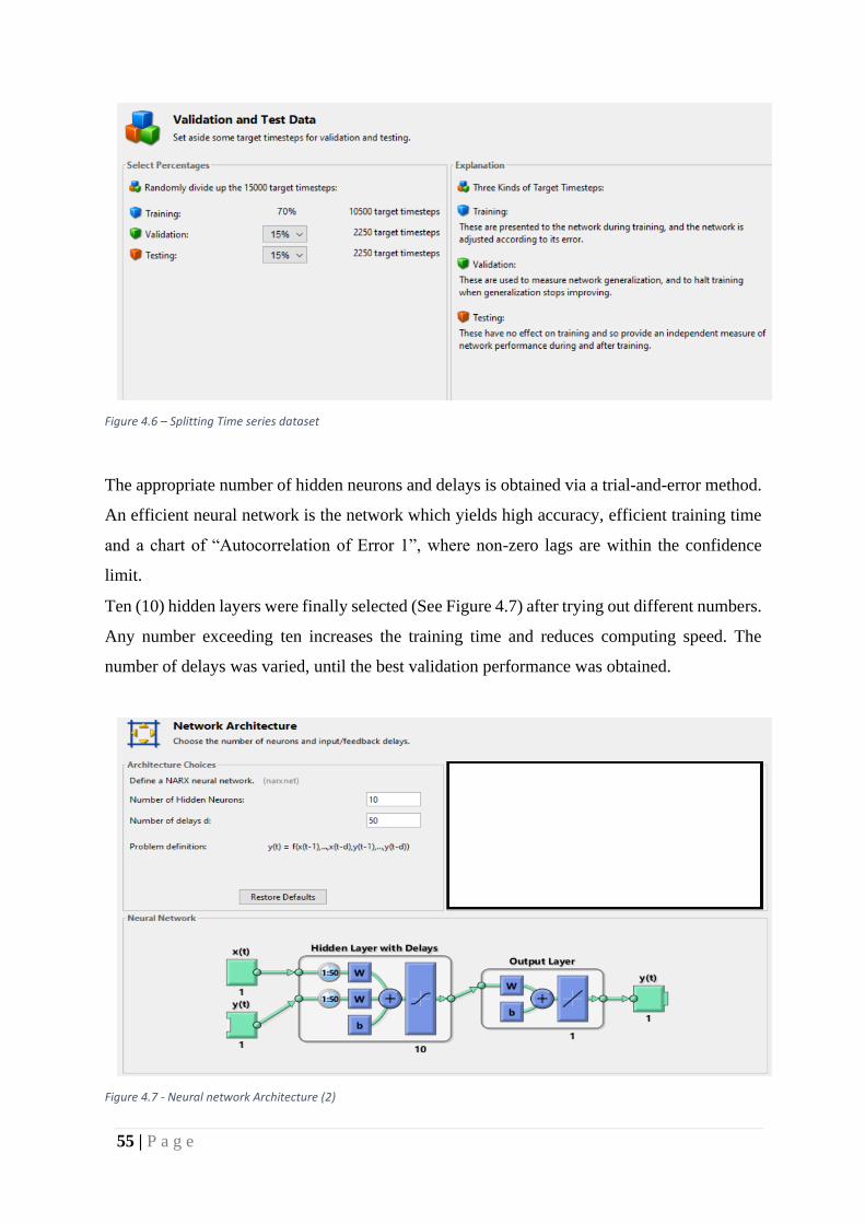
Figure 4.6 – Splitting Time series dataset

The appropriate number of hidden neurons and delays is obtained via a trial-and-error method.

An efficient neural network is the network which yields high accuracy, efficient training time

and a chart of “Autocorrelation of Error 1”, where non-zero lags are within the confidence

limit.

Ten (10) hidden layers were finally selected (See Figure 4.7) after trying out different numbers.

Any number exceeding ten increases the training time and reduces computing speed. The

number of delays was varied, until the best validation performance was obtained.

Figure 4.7 - Neural network Architecture (2)

56 | P a g e

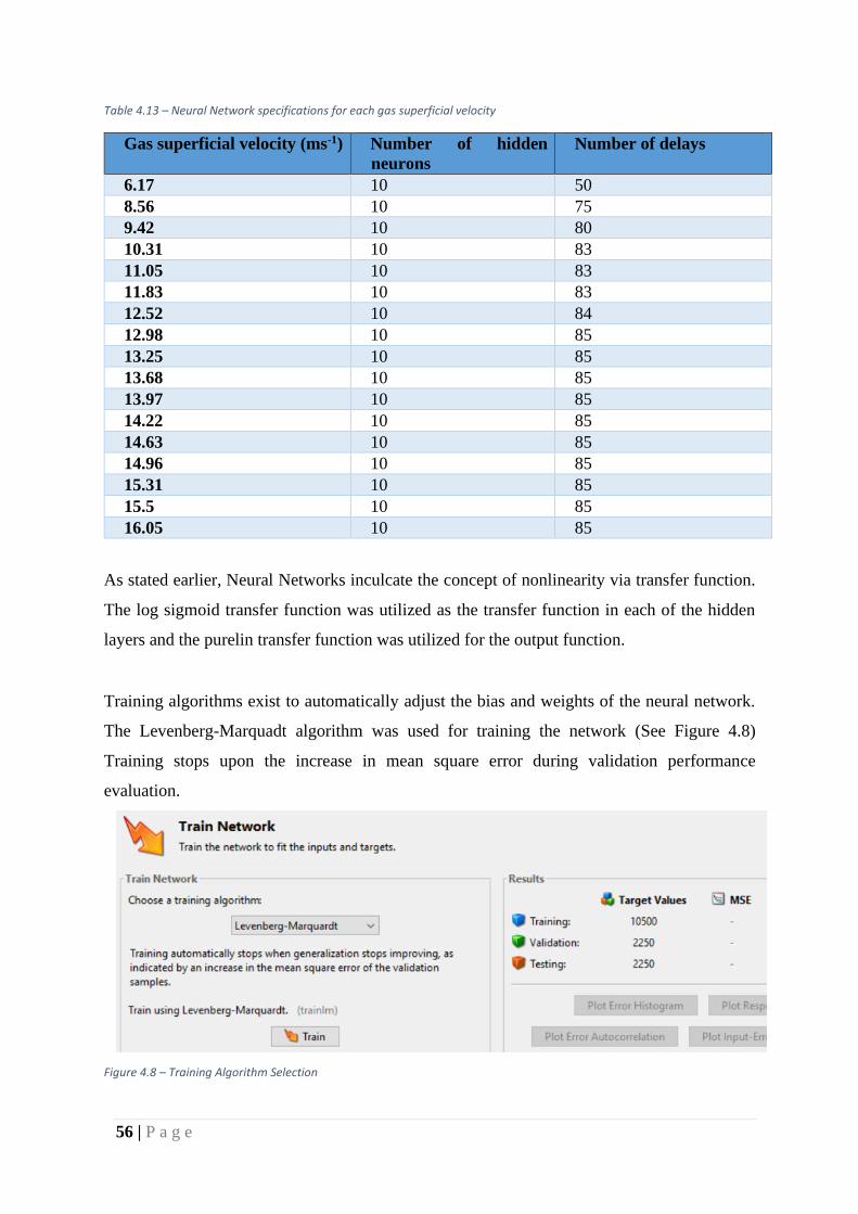
Table 4.13 – Neural Network specifications for each gas superficial velocity

Gas superficial velocity (ms-1) Number of hidden

neurons

Number of delays

6.17 10 50

8.56 10 75

9.42 10 80

10.31 10 83

11.05 10 83

11.83 10 83

12.52 10 84

12.98 10 85

13.25 10 85

13.68 10 85

13.97 10 85

14.22 10 85

14.63 10 85

14.96 10 85

15.31 10 85

15.5 10 85

16.05 10 85

As stated earlier, Neural Networks inculcate the concept of nonlinearity via transfer function.

The log sigmoid transfer function was utilized as the transfer function in each of the hidden

layers and the purelin transfer function was utilized for the output function.

Training algorithms exist to automatically adjust the bias and weights of the neural network.

The Levenberg-Marquadt algorithm was used for training the network (See Figure 4.8)

Training stops upon the increase in mean square error during validation performance

evaluation.

Figure 4.8 – Training Algorithm Selection

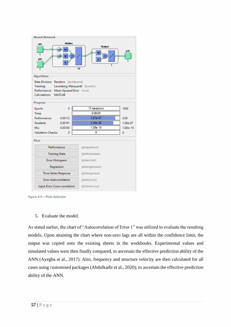
57 | P a g e

Figure 4.9 – Plots Selection

5. Evaluate the model.

As stated earlier, the chart of “Autocorrelation of Error 1” was utilized to evaluate the resulting

models. Upon attaining the chart where non-zero lags are all within the confidence limit, the

output was copied onto the existing sheets in the workbooks. Experimental values and

simulated values were then finally compared, to ascertain the effective prediction ability of the

ANN (Ayegba et al., 2017). Also, frequency and structure velocity are then calculated for all

cases using customised packages (Abdulkadir et al., 2020); to ascertain the effective prediction

ability of the ANN.

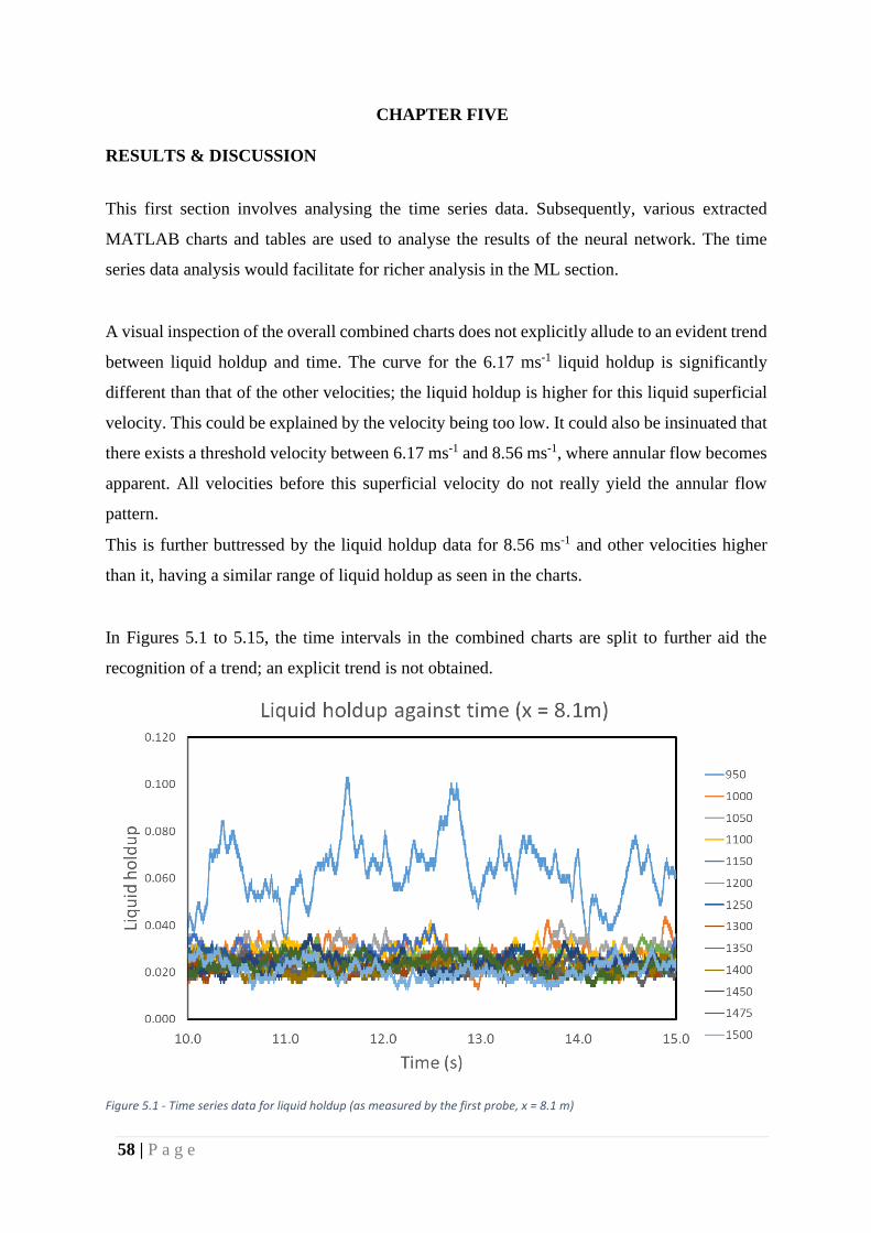
58 | P a g e

CHAPTER FIVE

RESULTS & DISCUSSION

This first section involves analysing the time series data. Subsequently, various extracted

MATLAB charts and tables are used to analyse the results of the neural network. The time

series data analysis would facilitate for richer analysis in the ML section.

A visual inspection of the overall combined charts does not explicitly allude to an evident trend

between liquid holdup and time. The curve for the 6.17 ms-1 liquid holdup is significantly

different than that of the other velocities; the liquid holdup is higher for this liquid superficial

velocity. This could be explained by the velocity being too low. It could also be insinuated that

there exists a threshold velocity between 6.17 ms-1 and 8.56 ms-1, where annular flow becomes

apparent. All velocities before this superficial velocity do not really yield the annular flow

pattern.

This is further buttressed by the liquid holdup data for 8.56 ms-1 and other velocities higher

than it, having a similar range of liquid holdup as seen in the charts.

In Figures 5.1 to 5.15, the time intervals in the combined charts are split to further aid the

recognition of a trend; an explicit trend is not obtained.

Figure 5.1 - Time series data for liquid holdup (as measured by the first probe, x = 8.1 m)

59 | P a g e

Figure 5.2 - Time series data for liquid holdup (as measured by the second probe, x = 8.3 m)

Figure 5.3 - Time series data for liquid holdup (as measured by the third probe, x = 8.5 m)

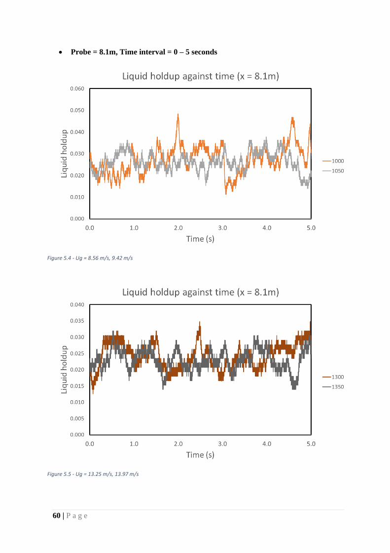
60 | P a g e

• Probe = 8.1m, Time interval = 0 – 5 seconds

Figure 5.4 - Ug = 8.56 m/s, 9.42 m/s

Figure 5.5 - Ug = 13.25 m/s, 13.97 m/s

61 | P a g e


-

Figure 5.6 - Ug = 8.56 m/s, 9.42 m/s

Figure 5.7 - Ug = 13.25 m/s, 13.97 m/s

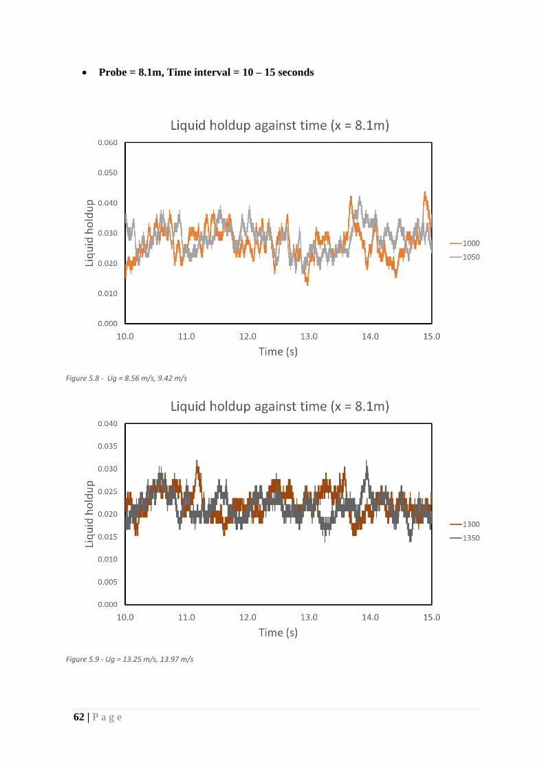
62 | P a g e


Figure 5.8 - Ug = 8.56 m/s, 9.42 m/s

Figure 5.9 - Ug = 13.25 m/s, 13.97 m/s

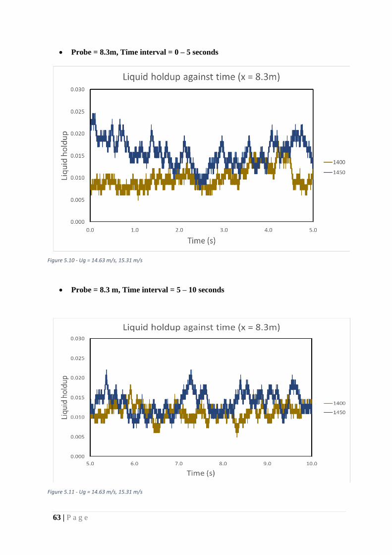
63 | P a g e


Figure 5.10 - Ug = 14.63 m/s, 15.31 m/s

• Probe = 8.3 m, Time interval = 5 – 10 seconds

Figure 5.11 - Ug = 14.63 m/s, 15.31 m/s

64 | P a g e


Figure 5.12 - Ug = 14.63 m/s, 15.31 m/s


Figure 5.13 - Ug = 13.97 m/s, 16.05 m/s

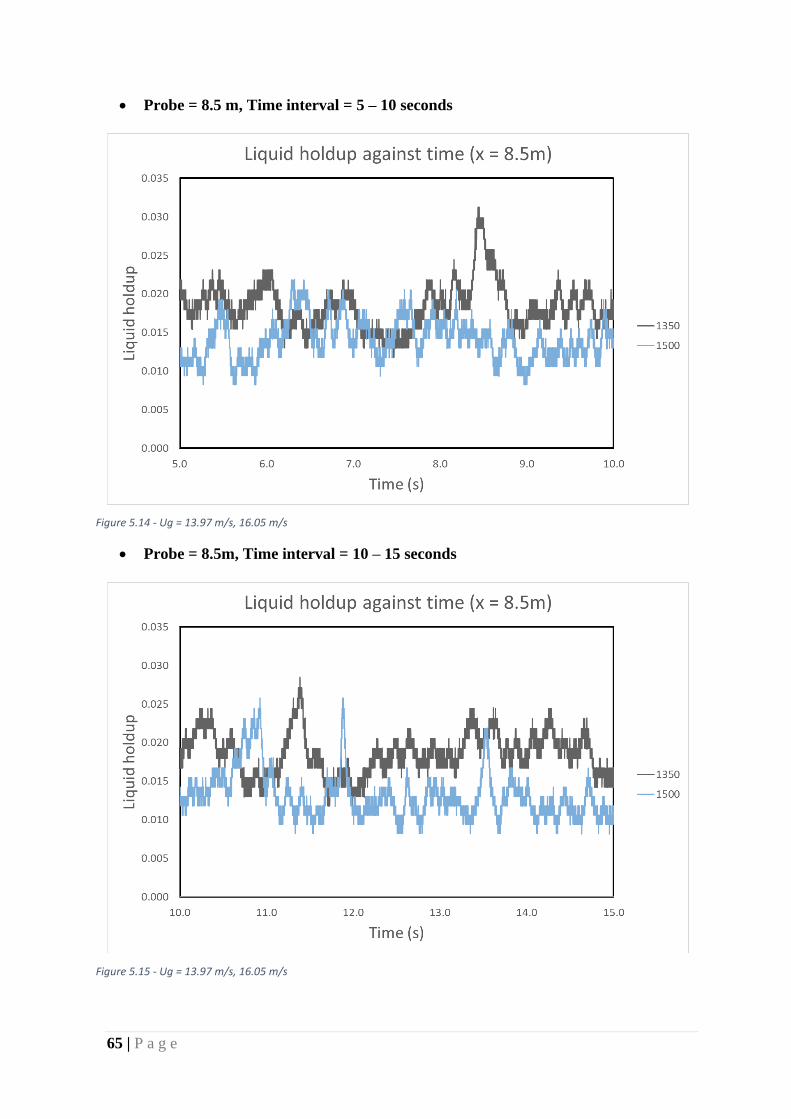
65 | P a g e


Figure 5.14 - Ug = 13.97 m/s, 16.05 m/s


Figure 5.15 - Ug = 13.97 m/s, 16.05 m/s

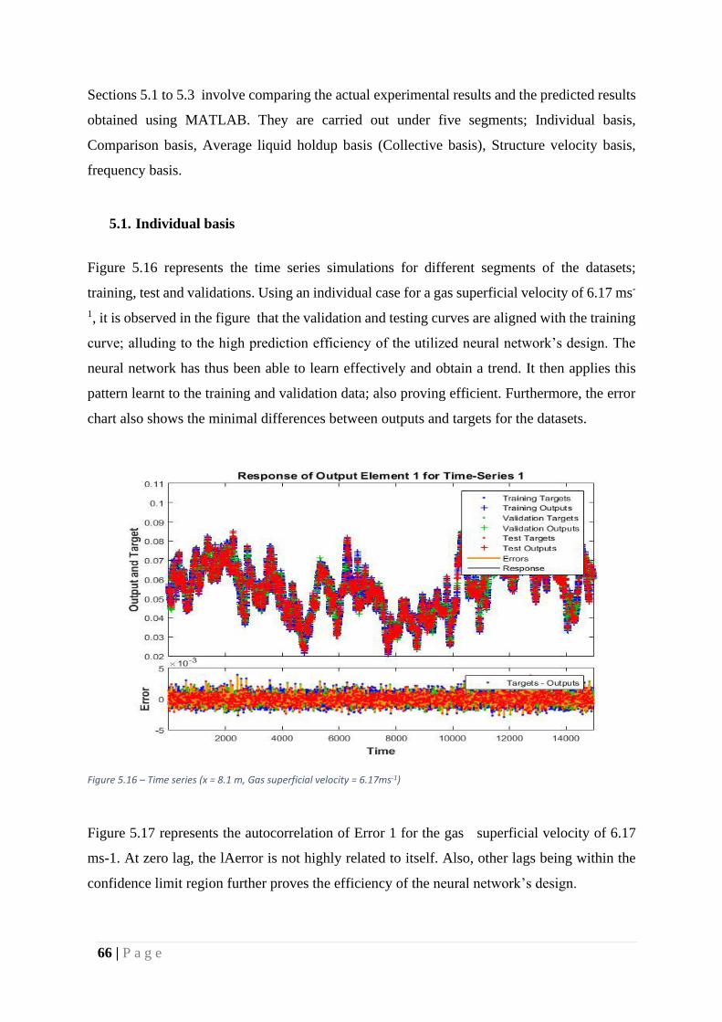
66 | P a g e

Sections 5.1 to 5.3 involve comparing the actual experimental results and the predicted results

obtained using MATLAB. They are carried out under five segments; Individual basis,

Comparison basis, Average liquid holdup basis (Collective basis), Structure velocity basis,

frequency basis.

5.1. Individual basis

Figure 5.16 represents the time series simulations for different segments of the datasets;

training, test and validations. Using an individual case for a gas superficial velocity of 6.17 ms-

1, it is observed in the figure that the validation and testing curves are aligned with the training

curve; alluding to the high prediction efficiency of the utilized neural network’s design. The

neural network has thus been able to learn effectively and obtain a trend. It then applies this

pattern learnt to the training and validation data; also proving efficient. Furthermore, the error

chart also shows the minimal differences between outputs and targets for the datasets.

Figure 5.16 – Time series (x = 8.1 m, Gas superficial velocity = 6.17ms-1)

Figure 5.17 represents the autocorrelation of Error 1 for the gas superficial velocity of 6.17

ms-1. At zero lag, the lAerror is not highly related to itself. Also, other lags being within the

confidence limit region further proves the efficiency of the neural network’s design.

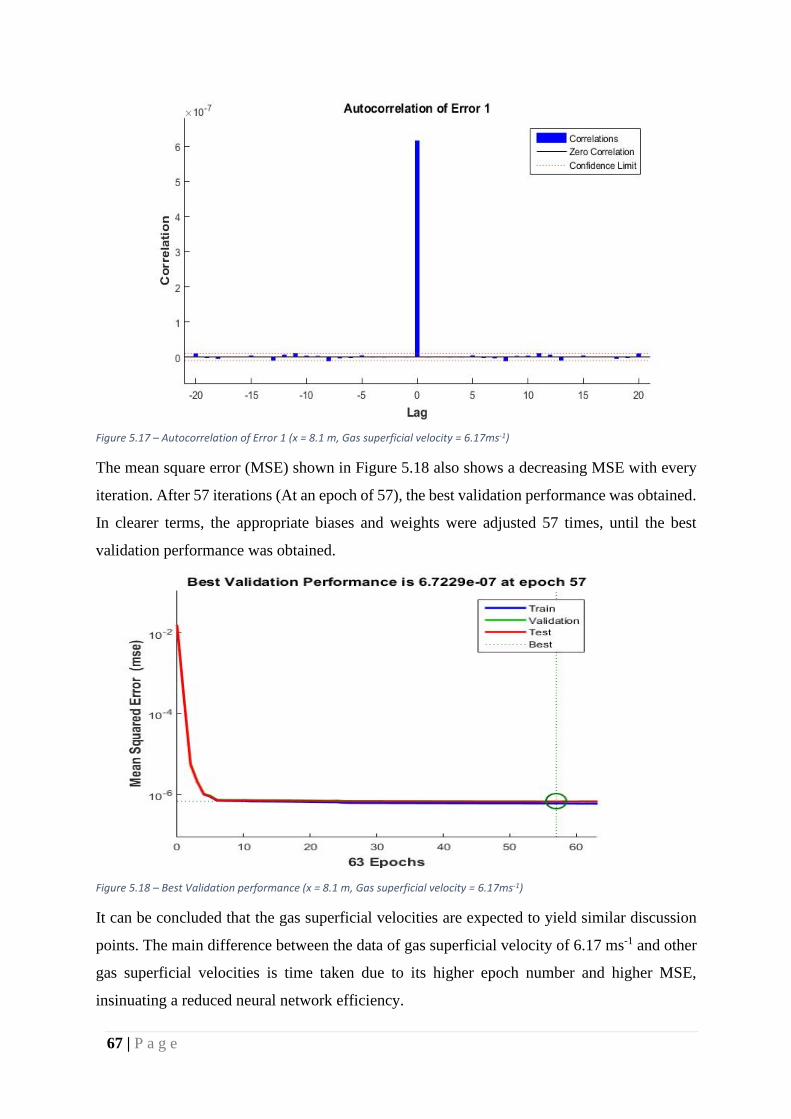
67 | P a g e

Figure 5.17 – Autocorrelation of Error 1 (x = 8.1 m, Gas superficial velocity = 6.17ms-1)

The mean square error (MSE) shown in Figure 5.18 also shows a decreasing MSE with every

iteration. After 57 iterations (At an epoch of 57), the best validation performance was obtained.

In clearer terms, the appropriate biases and weights were adjusted 57 times, until the best

validation performance was obtained.

Figure 5.18 – Best Validation performance (x = 8.1 m, Gas superficial velocity = 6.17ms-1)

It can be concluded that the gas superficial velocities are expected to yield similar discussion

points. The main difference between the data of gas superficial velocity of 6.17 ms-1 and other

gas superficial velocities is time taken due to its higher epoch number and higher MSE,

insinuating a reduced neural network efficiency.

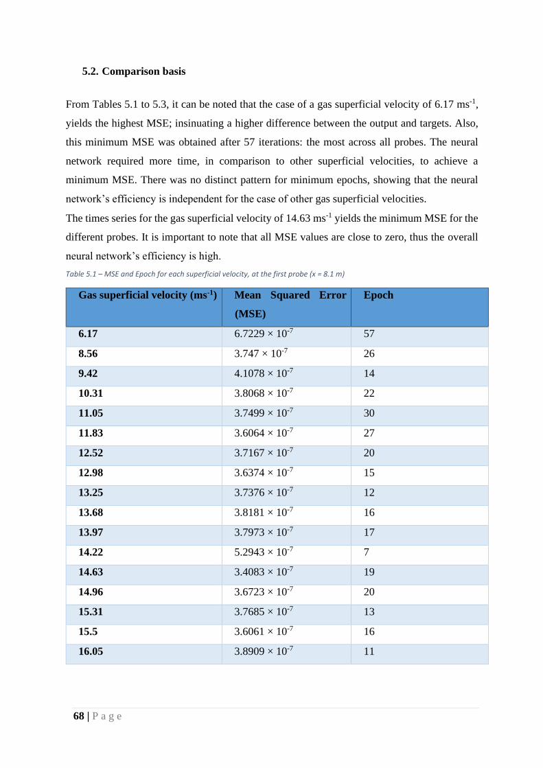
68 | P a g e

5.2. Comparison basis

From Tables 5.1 to 5.3, it can be noted that the case of a gas superficial velocity of 6.17 ms-1,

yields the highest MSE; insinuating a higher difference between the output and targets. Also,

this minimum MSE was obtained after 57 iterations: the most across all probes. The neural

network required more time, in comparison to other superficial velocities, to achieve a

minimum MSE. There was no distinct pattern for minimum epochs, showing that the neural

network’s efficiency is independent for the case of other gas superficial velocities.

The times series for the gas superficial velocity of 14.63 ms-1 yields the minimum MSE for the

different probes. It is important to note that all MSE values are close to zero, thus the overall

neural network’s efficiency is high.

Table 5.1 – MSE and Epoch for each superficial velocity, at the first probe (x = 8.1 m)

Gas superficial velocity (ms-1) Mean Squared Error

(MSE)

Epoch

6.17 6.7229 × 10-7 57

8.56 3.747 × 10-7 26

9.42 4.1078 × 10-7 14

10.31 3.8068 × 10-7 22

11.05 3.7499 × 10-7 30

11.83 3.6064 × 10-7 27

12.52 3.7167 × 10-7 20

12.98 3.6374 × 10-7 15

13.25 3.7376 × 10-7 12

13.68 3.8181 × 10-7 16

13.97 3.7973 × 10-7 17

14.22 5.2943 × 10-7 7

14.63 3.4083 × 10-7 19

14.96 3.6723 × 10-7 20

15.31 3.7685 × 10-7 13

15.5 3.6061 × 10-7 16

16.05 3.8909 × 10-7 11

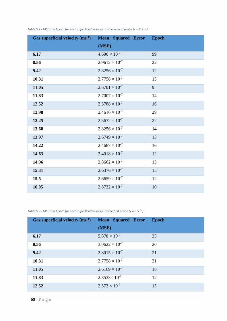
69 | P a g e

Table 5.2 - MSE and Epoch for each superficial velocity, at the second probe (x = 8.3 m)


(MSE)

Epoch

6.17 4.696 × 10-7 99

8.56 2.9612 × 10-7 22

9.42 2.8256 × 10-7 12

10.31 2.7758 × 10-7 15

11.05 2.6701 × 10-7 9

11.83 2.7007 × 10-7 14

12.52 2.3788 × 10-7 16

12.98 2.4616 × 10-7 29

13.25 2.5672 × 10-7 22

13.68 2.8256 × 10-7 14

13.97 2.6749 × 10-7 13

14.22 2.4687 × 10-7 16

14.63 2.4018 × 10-7 12

14.96 2.8662 × 10-7 13

15.31 2.6376 × 10-7 15

15.5 2.6659 × 10-7 12

16.05 2.8732 × 10-7 10

Table 5.3 - MSE and Epoch for each superficial velocity, at the first probe (x = 8.5 m)


(MSE)

Epoch

6.17 5.878 × 10-7 35

8.56 3.0622 × 10-7 20

9.42 2.8015 × 10-7 21

10.31 2.7758 × 10-7 21

11.05 2.6169 × 10-7 18

11.83 2.8533× 10-7 12

12.52 2.573 × 10-7 15

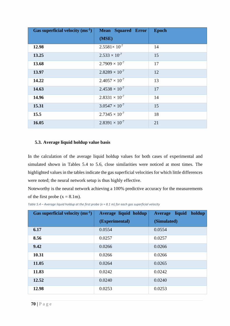
70 | P a g e


(MSE)

Epoch

12.98 2.5581× 10-7 14

13.25 2.533 × 10-7 15

13.68 2.7909 × 10-7 17

13.97 2.8289 × 10-7 12

14.22 2.4057 × 10-7 13

14.63 2.4538 × 10-7 17

14.96 2.8331 × 10-7 14

15.31 3.0547 × 10-7 15

15.5 2.7345 × 10-7 18

16.05 2.8391 × 10-7 21

5.3. Average liquid holdup value basis

In the calculation of the average liquid holdup values for both cases of experimental and

simulated shown in Tables 5.4 to 5.6, close similarities were noticed at most times. The

highlighted values in the tables indicate the gas superficial velocities for which little differences

were noted; the neural network setup is thus highly effective.

Noteworthy is the neural network achieving a 100% predictive accuracy for the measurements

of the first probe (x = 8.1m).

Table 5.4 – Average liquid holdup at the first probe (x = 8.1 m) for each gas superficial velocity

Gas superficial velocity (ms-1) Average liquid holdup

(Experimental)

Average liquid holdup

(Simulated)

6.17 0.0554 0.0554

8.56 0.0257 0.0257

9.42 0.0266 0.0266

10.31 0.0266 0.0266

11.05 0.0264 0.0265

11.83 0.0242 0.0242

12.52 0.0240 0.0240

12.98 0.0253 0.0253

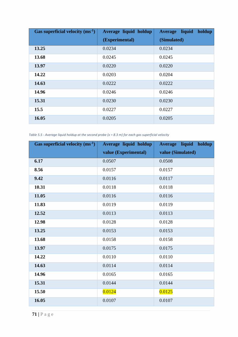
71 | P a g e


(Experimental)


(Simulated)

13.25 0.0234 0.0234

13.68 0.0245 0.0245

13.97 0.0220 0.0220

14.22 0.0203 0.0204

14.63 0.0222 0.0222

14.96 0.0246 0.0246

15.31 0.0230 0.0230

15.5 0.0227 0.0227

16.05 0.0205 0.0205

Table 5.5 - Average liquid holdup at the second probe (x = 8.3 m) for each gas superficial velocity


value (Experimental)


value (Simulated)

6.17 0.0507 0.0508

8.56 0.0157 0.0157

9.42 0.0116 0.0117

10.31 0.0118 0.0118

11.05 0.0116 0.0116

11.83 0.0119 0.0119

12.52 0.0113 0.0113

12.98 0.0128 0.0128

13.25 0.0153 0.0153

13.68 0.0158 0.0158

13.97 0.0175 0.0175

14.22 0.0110 0.0110

14.63 0.0114 0.0114

14.96 0.0165 0.0165

15.31 0.0144 0.0144

15.50 0.0124 0.0125

16.05 0.0107 0.0107

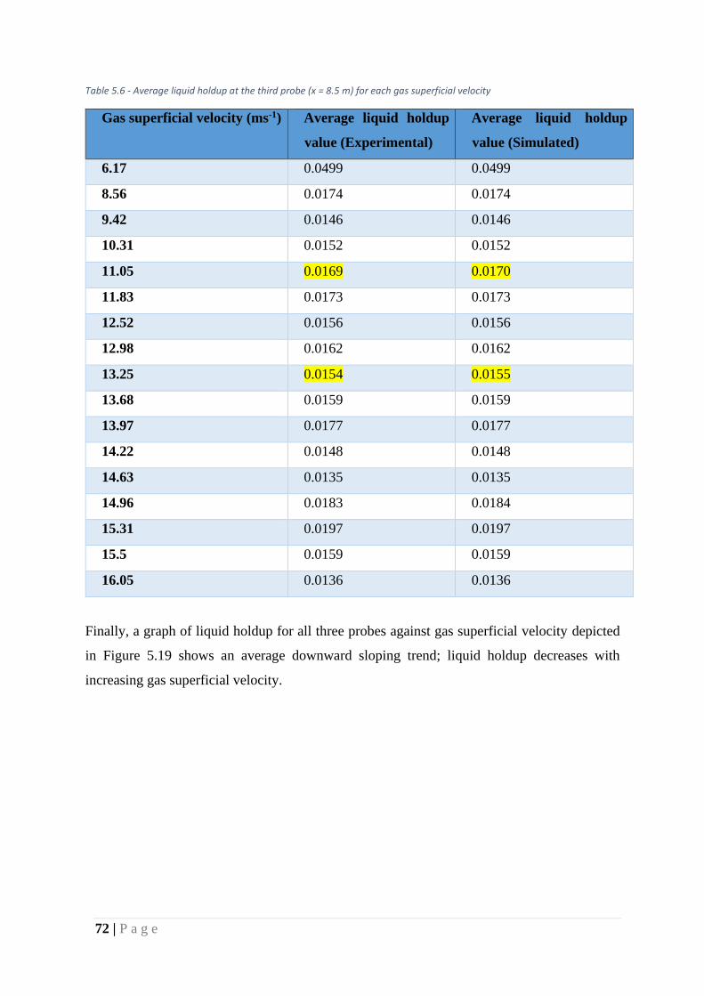
72 | P a g e

Table 5.6 - Average liquid holdup at the third probe (x = 8.5 m) for each gas superficial velocity


value (Experimental)


value (Simulated)

6.17 0.0499 0.0499

8.56 0.0174 0.0174

9.42 0.0146 0.0146

10.31 0.0152 0.0152

11.05 0.0169 0.0170

11.83 0.0173 0.0173

12.52 0.0156 0.0156

12.98 0.0162 0.0162

13.25 0.0154 0.0155

13.68 0.0159 0.0159

13.97 0.0177 0.0177

14.22 0.0148 0.0148

14.63 0.0135 0.0135

14.96 0.0183 0.0184

15.31 0.0197 0.0197

15.5 0.0159 0.0159

16.05 0.0136 0.0136

Finally, a graph of liquid holdup for all three probes against gas superficial velocity depicted

in Figure 5.19 shows an average downward sloping trend; liquid holdup decreases with

increasing gas superficial velocity.

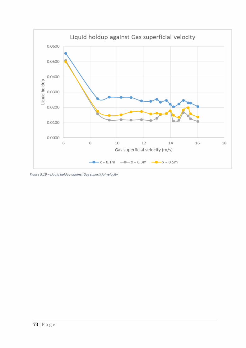
73 | P a g e

Figure 5.19 – Liquid holdup against Gas superficial velocity

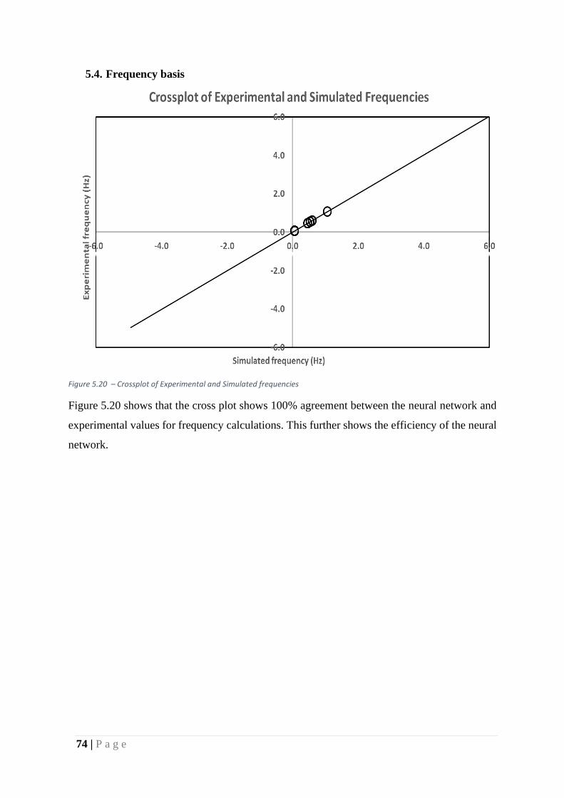
74 | P a g e

5.4. Frequency basis

Figure 5.20 – Crossplot of Experimental and Simulated frequencies

Figure 5.20 shows that the cross plot shows 100% agreement between the neural network and

experimental values for frequency calculations. This further shows the efficiency of the neural

network.

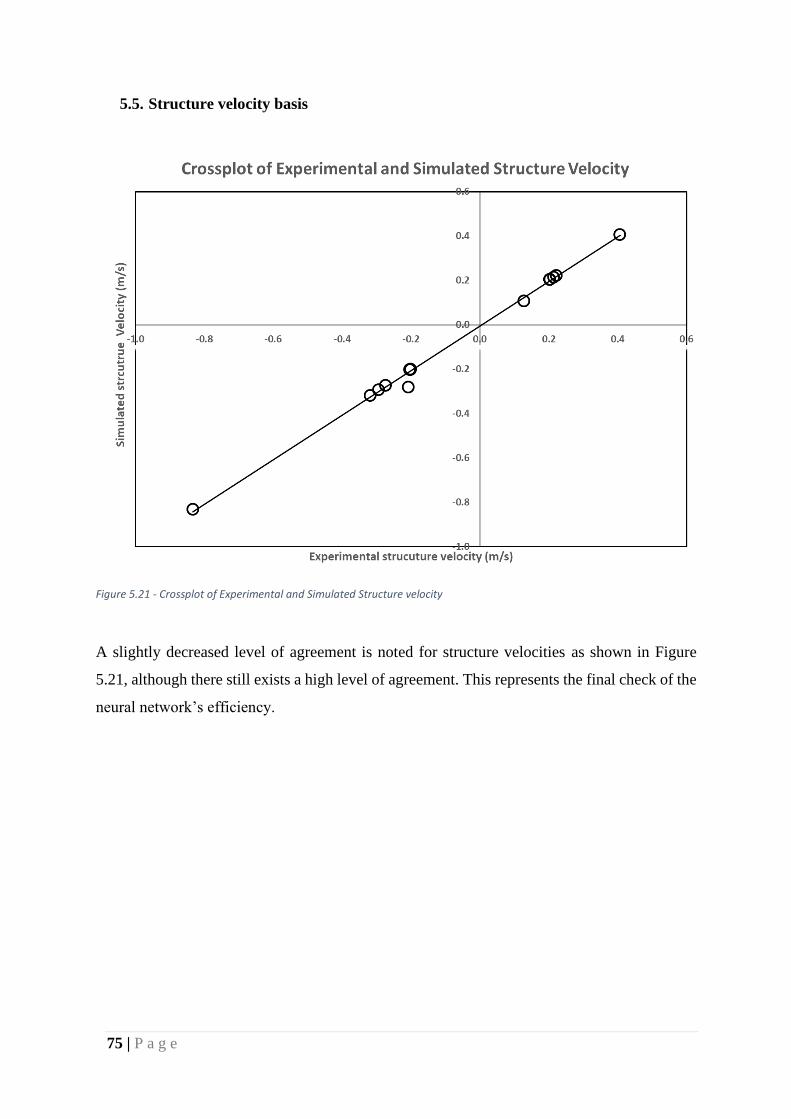
75 | P a g e

5.5. Structure velocity basis

Figure 5.21 - Crossplot of Experimental and Simulated Structure velocity

A slightly decreased level of agreement is noted for structure velocities as shown in Figure

5.21, although there still exists a high level of agreement. This represents the final check of the

neural network’s efficiency.

76 | P a g e

CHAPTER SIX

CONCLUSION & RECOMMENDATIONS

6.1. Summary and Conclusions

Lack of substantial literature exits for the prediction of liquid holdup and flow behaviour during

annular flow. A neural network of a specific design was able to accurately predict liquid holdup

during annular flow, in this research work. Furthermore, the utilized approach could be

modified as appropriate and used to solve other Flow Assurance problems.

In this research, experimental annular flow data containing liquid holdup against time was fed

into a neural network. Data represented the liquid holdup measurements at three different

probes, each located at different points across the air–water system. Also, liquid holdup was

measured for 17 different systems each having different gas superficial velocities, whilst the

liquid velocity was maintained in all cases. The neural network was trained via the Levenberg-

Marquadt algorithm in all cases.

It was noted that neural network architectures made up of a maximum of 10 hidden neurons

and a minimum of 50 delays accurately predicted liquid holdup values for all systems,

regardless of the probe location and liquid and gas superficial velocities. Furthermore,

prediction was carried out efficiently; reasonable time and memory was utilized in training,

testing and validating the neural network.

The neural network’s >90% predictive accuracy was validated by finding the average liquid

holdup in experimental and simulated cases; no differences in results were noted. Structural

velocity and frequency were also used to validate the neural network’s efficiency.

6.2. Recommendations

Future and more detailed research should attempt to focus on establishing relationships

between liquid holdup and time. The different time series charts in this research work portray

seasonality and trend; an equation should thus be able to provide accurate liquid holdup results.

Different neural network architectures where their independent variables could be inputted

(surface tension, gas superficial velocity liquid superficial velocity) should also be tested. This

would provide a better understanding on the modalities of neural networks. Such different

neural network setups need not be on only annular flow. Including other flow patterns would

77 | P a g e

help identify if results obtained in this research work are peculiar to only annular flow or could

be extended to other flow patterns.

In this research, only gas superficial velocity was varied; it would be advantageous to test the

neural network architectures on data where liquid superficial velocity is varied. The validation

performance would hint at where extra efforts need be directed. The training algorithm utilized

could also be changed and its effect on the neural network accuracy noted.

Finally, experimental data of different liquid-gas systems should be tested against neural

networks; findings could establish a direction for the utilization of machine learning for flow

assurance in the oil & gas sector.

Implementing neural networks in different manners as stated above, would provide extra

literature further enriching the few existing literature present.

78 | P a g e

REFERENCES

1. P.O. Ayegba, M. Abdulkadir, , V. Hernandez-Perez, I.S. Lowndes, B.J. Azzopardi

(2017) 'Applications of artificial neural network (ANN) method for performance

prediction of the effect of a vertical 90° bend on an air–silicone oil flow', Journal of the

Taiwan Institute of Chemical Engineers, 74(17), pp. 59 - 64.

2. Abdulkadir, M. (2020) Supervisor Meetings.

3. Ali and Tawfiq, F. (2019) Algorithm, Available

at: https://whatis.techtarget.com/definition/algorithm (Accessed: 14th August 2020).

4. Alpaydin, E. (2010) Introduction to Machine Learning, 2nd edn., United States of

America: MIT Press.

5. Baker, O. (1954) Simultaneous Flow of Oil and Gas, Oil and Gas Journal, 53, pp.185-

195.

6. Chauhan, N.S (2020) Decision Tree Algorithm, Explained, Available

at: https://www.kdnuggets.com/2020/01/decision-tree-algorithm-

explained.html (Accessed: 5th August 2020).

7. Chollet, F. (2017) Deep Learning with Python, United States of America: Manning

Publications.

8. G. F. Hewitt and D. N. Roberts. (1969) Studies of Two-Phase Flow Patterns by

Simultaneous Flash and XRay Photography, AERE-M2159

9. Geocities Liquid holdup, Available

at: http://www.geocities.ws/abouelsaoud/productionstorage/liquidholdup.pdf (Access

ed: 30th November 2017).

10. Golan, L.P. and Stenning, A.H. (1969) Two-Phase Vertical Flow Maps, Proc. Inst.

Mech. Eng. Vol. 184 (3C), pp. 110-116.

11. Guo, Y. (2017) The 7 Steps of Machine Learning, Available at:

https://towardsdatascience.com/the-7-steps-of-machine-learning

2877d7e5548e (Accessed: 14th October 2020).

12. Gupta, D. (2018) Mathematics for Machine Learning: Linear Regression & Least

Square Regression, Available at: https://towardsdatascience.com/mathematics-for-

machine-learning-linear-regression-least-square-regression-de09cf53757c

(Accessed: 18th September 2020).

https://whatis.techtarget.com/definition/algorithm

https://towardsdatascience.com/mathematics-for-machine-learning-linear-regression-least-square-regression-de09cf53757c

https://towardsdatascience.com/mathematics-for-machine-learning-linear-regression-least-square-regression-de09cf53757c

79 | P a g e

13. Hagan, T., Demuth, H., Beale, M. and Jesús, O. (2014) Neural Network Design, 2nd

edn., Online: Martin Hagan.

14. Izaugarat, E. (2018) Understanding Neural Networks: What, How and Why?, Available

at: https://towardsdatascience.com/understanding-neural-networks-what-how-and-

why-18ec703ebd31 (Accessed: 22nd October 2020).

15. Jacobs, T. (2020) 'Firm That Transforms Surface Properties With Lasers Wins Top

Prize at ATCE Startup Village', Journal of Petroleum Technology, (), pp. [Online].

Available at: https://pubs.spe.org/en/jpt/jpt-article-detail/?art=7737 (Accessed: 14th

October 2020).

16. Luhaniwal, V. (2019) Analyzing different types of activation functions in neural

networks — which one to prefer?, Available

at: https://towardsdatascience.com/analyzing-different-types-of-activation-functions-

in-neural-networks-which-one-to-prefer-e11649256209 (Accessed: 22nd October

2020).

17. Mandhane, J.M., Gregory, G.A., and Aziz, K. (1974) A flow pattern map for gas-liquid

flow in horizontal pipes. International Journal of Multiphase Flow 1, 537-553.

18. Marsland, S. (2015) MACHINE LEARNING An Algorithmic Perspective, 2nd edn.,

United States of America: CRC Press.

19. Mayo, M. (2017) Neural Network Foundations, Explained: Updating Weights with

Gradient Descent & Backpropagation, Available

at: https://www.kdnuggets.com/2017/10/neural-network-foundations-explained-

gradient-descent.html (Accessed: 11th September 2020).

20. Michaelides, E., Crowe, C. and Schwarzkopf, J. (2017) Multiphase Flow Handbook,

2nd edn., United States of America: Taylor & Francis Group.

21. Nilsson, N. J. (2005). Introduction to Machine Learning. Stanford, CA.

22. Oil & Gas IQ Editor (2018) What is flow assurance?, Available

at: https://www.oilandgasiq.com/oil-and-gas-production-and-operations/news/what-

is-flow-assurance (Accessed: 1st September 2020).

23. Paran, M. and Palermo, T. (2020) Deep Offshore Flow Assurance, Available

at: https://www.ep.total.com/en/areas/deep-offshore/flow-assurance-sensitive-issue-

any-oil-development-project (Accessed: 2nd October 2020).

24. Petroleum Economist (2006) The billion-dollar blockage, Available

at: http://dev.petroleum-economist.com/articles/upstream/technology/2006/the-

billion-dollar-blockage (Accessed: 15th September 2020).

https://www.oilandgasiq.com/oil-and-gas-production-and-operations/news/what-is-flow-assurance

https://www.oilandgasiq.com/oil-and-gas-production-and-operations/news/what-is-flow-assurance

https://www.ep.total.com/en/areas/deep-offshore/flow-assurance-sensitive-issue-any-oil-development-project

https://www.ep.total.com/en/areas/deep-offshore/flow-assurance-sensitive-issue-any-oil-development-project

80 | P a g e

25. Sun, B. (2016) Multiphase Flow in Oil and Gas Well Drilling, Singapore: Wiley &

Sons (Asia) Pte Ltd Pacific, John.

26. Taitel, Y. and Dukler, A. E. (1976) A Model Of Predicting Flow Regime Transitions In

Horizontal And Near Horizontal Gas-Liquid Flow. AIChE J., 22:47–55

27. Tay, K. (2017) Terminology Explained: What is multiphase flow?, Available

at: https://blogs.dnvgl.com/software/2017/06/terminology-explained-multiphase-

flow/ (Accessed: 30th June 2017).

28. Theobald, O. (2017) Machine Learning For Absolute Beginners, 2nd edn., : Oliver

Theobald.

29. Wasserman, L. (2004) All of Statistics: A Concise Course in Statistical Inference,

United States of America: Springer Texts in Classics.

30. Whalley, P. B. (1987) Boiling, condensation, and gas-liquid flow. Oxford Oxfordshire.

New York: Clarendon Press; Oxford University Press

31. Yale University (2018) Multiple Linear Regression, Available

at: http://www.stat.yale.edu/Courses/1997-98/101/linmult.htm (Accessed: 5th August

2020).

32. Yiu, T. (2019) Understanding Random Forest, Available

at: https://towardsdatascience.com/understanding-random-forest-

58381e0602d2 (Accessed: 9th August 2020)

utilization of machine learning for flow assurance in …

Documents