utilizing micro simulation to evaluate the safety and...
TRANSCRIPT
Utilizing Micro Simulation to Evaluate the Safety and Efficiency of the Expressway System
Jaeyoung Lee, Ph.D., PI
Research Assistant Professor
Mohamed Abdel-Aty, Ph.D., Co-PI Professor & Chair
Ling Wang, Ph.D.
Department of Civil, Environmental and Construction Engineering
University of Central Florida
ii
Utilizing Micro Simulation to Evaluate the Safety and Efficiency of the Expressway System
Jaeyoung Lee, Ph.D., PI
Safety Program Director & Research Assistant Professor
Center for Advanced Transportation Systems Simulation
Department of Civil, Environmental and Construction Engineering
University of Central Florida
Mohamed Abdel-Aty, Ph.D., Co-PI
Pegasus Professor & Chair
Department of Civil, Environmental and Construction Engineering
University of Central Florida
Ling Wang, Ph.D.
Post-doctoral Associate
Department of Civil, Environmental and Construction Engineering
University of Central Florida
A Report on Research Sponsored by SAFER-SIM
August 2016

iii
Table of Contents
Table of Contents ............................................................................................................................ iii
List of Figures .................................................................................................................................... v
List of Tables .................................................................................................................................... vi
Abstract .......................................................................................................................................... vii
1 Introduction ............................................................................................................................... 1
2 Literature Review ....................................................................................................................... 4
2.1 Crash Analyses.................................................................................................................. 4
2.2 ATM Strategies ................................................................................................................. 6
3 Big Data Collection and Processing .......................................................................................... 10
3.1 Crash Data ...................................................................................................................... 11
3.2 Traffic Data ..................................................................................................................... 16
3.3 Road Geometric Characteristics Data ............................................................................ 19
3.4 Weather Data ................................................................................................................. 21
4 Safety Analysis of Expressway System ..................................................................................... 22
4.1 Introduction ................................................................................................................... 22
4.2 Data Preparation ............................................................................................................ 23
4.3 Methodology .................................................................................................................. 27
4.3.1 Case-control Design .......................................................................................... 27
4.3.2 Crash Prediction Models ................................................................................... 29
4.3.3 Model Comparison ............................................................................................ 31
4.4 Model Estimation and Comparison ................................................................................ 34
4.4.1 Crash Prediction Model ..................................................................................... 34
4.4.2 Model Comparison Results ............................................................................... 37
4.5 Summary ........................................................................................................................ 39
5 Real-time Safety Analysis for Weaving Segments ................................................................... 41
5.1 Introduction ................................................................................................................... 41
5.2 Methodology .................................................................................................................. 43

iv
5.3 Data Collection ............................................................................................................... 44
5.4 Crash Prediction Model .................................................................................................. 45
5.5 Summary ........................................................................................................................ 47
6 Microsimulation Network Building .......................................................................................... 49
6.1 Study Segment Identification ......................................................................................... 49
6.1.1 Key expressway ................................................................................................. 49
6.1.2 Key segment ...................................................................................................... 51
6.2 Network Coding ............................................................................................................. 53
6.3 Field Traffic Data Input ................................................................................................... 54
6.4 VISSIM Network Calibration and Validation .................................................................. 59
6.5 Summary ........................................................................................................................ 63
7 Traffic Safety Improvement for a Congested Weaving Segment ............................................ 64
7.1 Introduction ................................................................................................................... 64
7.2 ATM Strategy Algorithm ................................................................................................. 64
7.2.1 Ramp Metering Algorithm ................................................................................ 64
7.2.2 Variable Speed Limit Strategy ........................................................................... 65
7.3 Experiment Design ......................................................................................................... 66
7.4 Evaluation of ATM Strategies ......................................................................................... 69
7.5 Summary ........................................................................................................................ 75
8 Conclusion ................................................................................................................................ 77
APPENDIX A MVDS System and Lane Configuration ...................................................................... 80
APPENDIX B Expressway Hourly Volume........................................................................................ 88
APPENDIX C Expressway Mainline Congestion .............................................................................. 91
References ...................................................................................................................................... 96

v
List of Figures
Figure 3.1 – Studied expressways. ................................................................................................ 10
Figure 3.2 – CFX expressway network in GIS. ................................................................................ 12
Figure 3.3 – Total crashes in Orange County in 2013. ................................................................... 12
Figure 3.4 – Initial selection of expressway crashes ..................................................................... 14
Figure 3.5 – Final selection of expressway crashes. ...................................................................... 14
Figure 3.6 – Crash match on mainline, ramp and toll plaza lanes. ................................................ 15
Figure 3.7 – Deployment of MVDS sensors on the expressway network. .................................... 16
Figure 4.1 – Different segment types. ........................................................................................... 24
Figure 4.2 – Model results transformation. .................................................................................. 32
Figure 4.3 – Hourly volume and crash frequency. ......................................................................... 38
Figure 5.1 – Weaving segment traffic movements. ...................................................................... 41
Figure 6.1 – Weekday hourly volume of SR 408 westbound in August 2015. .............................. 50
Figure 6.2 – Weekday occupancy of SR 408 westbound. .............................................................. 51
Figure 6.3 – Weekday hourly volume in 2015. .............................................................................. 52
Figure 6.4 – Coded freeway section with background image. ...................................................... 53
Figure 6.5 – Data collection points in VISSIM. ............................................................................... 54
Figure 6.6 – Average 5-min volume on Thursdays in August 2015. .............................................. 56
Figure 6.7 – Cumulative speed distribution for mainline. ............................................................. 57
Figure 6.8 – Mainline desired speed distribution of (a) PC and (b) HGV. ..................................... 58
Figure 7.1 – Studied weaving segment microsimulation network. ............................................... 68
Figure 7.2 – Crash risk for different cases ..................................................................................... 74

vi
List of Tables
Table 3.1 – Key words used for expressway crash selection. ........................................................ 13
Table 3.2 – Crash number of expressways. ................................................................................... 15
Table 3.3 – SR 408 eastbound MVDS system and lane configuration. .......................................... 18
Table 3.4 – RCI data structure. ...................................................................................................... 20
Table 4.1 – Descriptive analysis of the geometric characteristic. ................................................. 25
Table 4.2 – Crash characteristic on each segment type. ............................................................... 26
Table 4.3 – Crash prediction model. .............................................................................................. 35
Table 4.4 – Model comparison results. ......................................................................................... 37
Table 5.1 – List of variables. .......................................................................................................... 45
Table 5.2 – Real-time crash estimation model for weaving segments. ........................................ 46
Table 6.1 – Sample of GEH values for calibration. ........................................................................ 60
Table 6.2 – Speed differences for validation. ................................................................................ 62
Table 7.1 – ATM scenarios. ............................................................................................................ 69
Table 7.2 – ATM simulation results ............................................................................................... 71

vii
Abstract
Expressways play a vital role in serving mega-cities, and the safety of expressways is extremely
important. In order to explore the crash mechanisms of expressways, previous studies have
mainly utilized average daily traffic (ADT) as a major contributing factor. In recent years, several
researchers also adopted average hourly traffic (AHT) and microscopic traffic at five-minute
intervals in expressway safety analyses. Nevertheless, there have been no studies, which have
compared the performance of all three factors: ADT, AHT, and microscopic traffic.
This study collected data from three expressways in Central Florida, including traffic data at one-
minute intervals, detailed crash information, and geometric characteristics. A Bayesian Poisson-
lognormal model was estimated for total crash frequency using ADT, a Bayesian multilevel
Poisson-lognormal model was built for hourly crash frequency prediction using AHT, and a
Bayesian multilevel logistic regression model was developed for real-time safety analysis using
microscopic traffic indicators at five-minute intervals. The modeling results showed that the
crash-contributing factors found by different models were comparable but not the same. Four
variables, i.e., the logarithm of volume, segment length, number of lanes, and existence of
weaving segments, were found to be positively significant in the three models, and four other
variables were only significant in one or two models. The ADT-based, AHT-based, and five-
minute-based models were used to predict safety conditions at different levels: total, hourly,
and five-minute intervals. The results indicated that the AHT-based crash-estimation model
performed the best in predicting total and hourly crash frequency, and that the real-time crash
prediction model was the best in identifying crash events for dangerous segments at five-minute
intervals. The AHT was recommended for future long-term traffic safety analysis, and traffic at
five-minute intervals was suggested for the implementation of active traffic management
(ATM).
Since the existence of weaving segments was found to be significantly related to crash potential
in all three crash analyses models, crash-contributing factors of weaving segments were further
studied using real-time safety analysis, which implements traffic at five-minute intervals to
predict crash potential. This study presents a logistic regression model for crashes at expressway
weaving segments using crash data, geometric data, traffic data at one-minute intervals, and
weather data. The results show that the speed difference between the beginning and the end of
the weaving segment and the logarithm of volume have significant impacts on the crash risk of
the following five to ten minutes for weaving segments. The configuration is also an important
factor. The weaving segment, in which there is no need for on- or off-ramp traffic to change
lanes, presents a high crash risk because there are more traffic interactions and greater speed
differences between weaving and non-weaving traffic. Meanwhile, weaving influence length,
which measures the distance at which weaving turbulence no longer has impact, is found to be
positively related to the crash risk at the 5% confidence interval. In addition to traffic and
geometric factors, the wet pavement surface condition significantly increases the crash risk
since vehicles are more likely to be out of control and need longer braking distances on wet
pavement. Once the crash mechanism of weaving segments was found, the safety condition of
weaving segments could be estimated using traffic, geometry, and weather factors at five-
minute intervals.

viii
This study focused on the safety of a congested weaving segment, which has a high crash
potential. Various ATM strategies were tested in microscopic simulation (VISSIM) through the
Component Object Model (COM) interface. The strategies included ramp metering (RM)
strategies, variable speed limit (VSL) strategies, and an integrated RM and VSL (RM-VSL)
strategy. Overall, the results showed that the ATM strategies were able to improve the safety of
the studied weaving segment. The modified ALINEA RM algorithms, which took both lane
occupancy and safety into consideration, outperformed the traditional ALINEA algorithm from a
safety point of view but at the expense of average travel time. The 45 mph VSLs, which were
located at the upstream of the studied weaving segment, significantly enhanced the safety
without notably increasing the average travel time. In order to reduce the average travel time of
the modified ALINEA RM and maintain its impact on safety, the modified ALINEA RM was
adjusted to control queue length and was integrated with the 45 mph VSL strategy. The
simulation results have proved that the consolidated RM-VSL approach yields slightly lower total
crash risks, but provides much lower average travel times than the modified ALINEA.
Overall, the existence of a weaving segment would significantly increase crash potential, and the
traffic at five-minute intervals was suitable for the implementation of ATM. Based on these two
findings, a congested weaving segment was chosen to test the impact of ATM on safety in real
time through microscopic simulation. The result showed that ATM was able to significantly
improve the safety of the studied weaving segment.

1 Utilizing Micro Simulation to Evaluate the Safety and Efficiency of the Expressway System
1 Introduction
Expressways play a vital role in serving mega-cities. They increase the travel speed and reduce
the travel time for daily traffic, especially for medium to long trips. If a crash occurs on an
expressway, it might bring about two serious consequences: 1) a more severe crash because
crash severity is highly related to speed limits, and the speed limits on expressways are usually
high; and 2) more congestion because expressways are access controlled, and it might be hard
for vehicles to easily change their route. Hence, reducing the crash potential of an expressway is
a worthwhile goal.
Previous safety analyses of expressways were mainly based on average daily traffic (ADT). In
recent years, with the development of data collection technologies and data processing
capabilities, more detailed traffic data, for example, average hourly traffic (AHT) and
microscopic traffic data at five-minute intervals, has become available. However, there have not
been enough studies, which compare these types of safety analyses, which are based on
different traffic data.
Different expressway segment types have different crash potentials. Meanwhile, crash
characteristics on different segment types is not the same. When practitioners set out to
improve the safety of an expressway, it is hard to take the whole expressway as a subject
because not all segments experience high crash frequencies, and because budgets are always
limited. Hence, there is a need to first find the most dangerous segment type. Then, the crash-
contributing factors of the most dangerous segment type should be closely explored.
Once the crash-contributing factors have been found, several countermeasures can be applied
to expressways to improve traffic safety. One of the possible countermeasures is active traffic
management (ATM), which is able to dynamically manage roadway facilities to change the traffic
conditions and further improve the safety of an expressway segment. In this project, to test the
impact of ATM on the safety of expressway segments, microscopic simulation was used. The
simulation is a cost-effective way to evaluate traffic safety in simulated scenarios, which allows
researchers and practitioners to test proposed improvement strategies. VISSIM is a widely used
microscopic road traffic simulation that is able to simulate the behavior of individual vehicles.
Hence, the simulated traffic network can be analyzed in detail. Additionally, in VISSIM, an
interface (the Component Object Model interface) is offered. Through the interface, users are
able to manipulate the attributes of internal objectives dynamically, such as speed limit and
ramp signal timing.
The main objective of this study was to improve the safety of an expressway system based on
safety analysis and microscopic simulation. To achieve the proposed objective, several tasks
were carried out.
Task 1: Evaluating the stability of the three types of safety analyses in identifying the
important contributing factors and their ability to use the identified variables to predict
safety conditions;

2 Utilizing Micro Simulation to Evaluate the Safety and Efficiency of the Expressway System
Task 2: Identifying the most dangerous expressway segment type based on safety
analyses using ADT, AHT, and microscopic data;
Task 3: Exploring the crash mechanism of the most dangerous expressway segment
type using real-time safety analysis;
Task 4: Building a well-calibrated and validated VISSIM network for an expressway
segment with high crash potential; and
Task 5: Testing the impact of ATM on the safety of the expressway segment identified
by Task 4.
Following this chapter, this report begins with a literature review on existing crash analysis and
ATM strategies in Chapter 2. Chapter 3 describes the data that were collected, including crash,
traffic, road geometric characteristics, and weather data. Chapter 4 focuses on safety analysis of
an expressway system based on traffic data aggregated at different levels: ADT, AHT, and
microscopic traffic. Chapter 5 conducted a real-time safety analysis for weaving segments, which
were identified as the most dangerous segment type by Chapter 4. Chapter 6 and 7 build a
microscopic simulation, VISSIM network for a congested weaving segment and apply ATM to
reduce the crash risk on the segment. Conclusions are summarized in Chapter 8.
3 Utilizing Micro Simulation to Evaluate the Safety and Efficiency of the Expressway System
2 Literature Review
This chapter presents the literature review in two parts: crash analyses and ATM strategies. In
the first part, crash analyses based on different traffic data are summarized to illustrate which
crash analysis might be suitable in safety analysis of expressway segments. In the second part,
two main ATM strategies, i.e., variable speed limit (VSL) and ramp metering (RM), have been
reviewed with a focus of the impact of ATM on traffic safety.
2.1 Crash Analyses
The cause-effect relationship between crashes and traffic conditions has been widely explored
based on ADT or annual average daily traffic (AADT). However, some researchers have stated
that the cause-effect relationship actually should be between a crash and the traffic conditions
prevailing near the time of crash occurrence, or else there might be a biased result due to the
implementation of AADT (Mensah & Hauer, 1998). Hence, AHT and microscopic traffic data at
five-minute intervals, which are closer to the time of crash occurrence than AADT, have been
used in crash analysis.
Average-hourly-traffic-based traffic safety studies were first conducted by Gwynn (1967). The
author found a U-shape relationship between crash rate and hourly volume: high crash rates
occurred at low and high hourly volumes and low crash rates at median hourly volumes. Later,
Ceder (1982) used power functions to examine the relationship between hourly traffic flows and
hourly crash rate because it was noted that ADT failed to explain the relationship between
traffic and crashes. In that study, different crash types (single- and multi-vehicle crashes) under
different traffic conditions (free- and congested-flow conditions) were studied separately. Then,
Persaud and Dzbik (1993) implemented generalized linear models and the empirical Bayesian
method to estimate crash frequency using hourly volume and ADT individually. However, in
their study, hourly traffic volumes were estimated on the basis of ADT. Martin (2002) explored
the relationship between crash rates and hourly volume and investigated the impact of volume
on crash severity.
Other hourly traffic parameters were also used to estimate hourly crashes. Lord et al. (2005)
applied hourly vehicle density and volume over capacity (v/c) in hourly crash frequency
prediction for rural and urban freeways. Their results showed that vehicle density and v/c ratio
were positively related to hourly crash frequency. Zhou and Sisiopiku (1997) used parabolic
equations to explain the relationship between v/c and crash rates for different crash types, for
example, multi-vehicle crashes and rear-end crashes. Chang et al. (2000) explored the
relationship between crash rate and hourly v/c. In their research, three types of freeway
segments were studied: basic freeway sections, tunnel sections, and toll gate sections. U-shape
relationships between crash rate and hourly v/c were also found for these three sections.
Compared to the hourly crash study, there are many more real-time safety studies. It has
become one of the most heavily studied traffic safety topics, since it was first examined in 1995
(Madanat and Liu, 1995). The subjects of real-time safety studies covered freeway mainlines
(Lee et al., 2002; Abdel-Aty et al., 2004; Pande et al., 2005), ramp vicinities (Hossain &
Muromachi, 2013a, b), ramps (Lee & Abdel-Aty, 2006; Wang et al., 2015b), and weaving
4 Utilizing Micro Simulation to Evaluate the Safety and Efficiency of the Expressway System
segments (Wang et al., 2015a). With more and more efforts in real-time safety analysis,
researchers explored different crash types in real time, including single-vehicle crashes and
multi-vehicle crashes (Yu & Abdel-Aty, 2013); explored crash-contributing factors under
different conditions, i.e., high- and low-speed conditions (Abdel-Aty et al., 2005). Crash
contributing factors discovered by former studies mainly included traffic (Hossain & Muromachi,
2013b), roadway geometric characteristics (Yu & Abdel-Aty, 2013), and weather (Abdel-Aty &
Pemmanaboina, 2006).
Almost all previous real-time safety analyses implemented case-control design to randomly
select some non-crash events to represent the non-crash population. The main reason for the
wide use of case-control design was that the number of non-crash events is always much
greater than that of crash events. Some of these studies adopted the matched-case-control
design to exclude the impact of geometry and time of day on crash occurrence (Pande et al.,
2005; Abdel-Aty & Pemmanaboina, 2006). The main statistical method of real-time crash
estimation is the logistic regression model (Abdel-Aty & Pemmanaboina, 2006; Hourdos et al.,
2006; Zheng et al., 2010). Additionally, several data mining methods have been used: Bayesian
belief net (Hossain & Muromachi, 2013a, b), support vector machine (Qu et al., 2012), and
multilayer perceptron neural network (Pande et al., 2011). The data mining method may provide
better model performance, but on the other hand, it might not be able to provide the
quantitative impact of a significant variable on crash occurrence.
To summarize, AHT-based and real-time safety analyses might outperform ADT-based safety
studies; there have been several hourly and real-time safety studies, but little to no research has
compared ADT-based, AHT-based, and five-minute-based crash analyses. Case-control design
has been widely implemented in real-time safety analyses.
2.2 ATM Strategies
Active traffic management is mainly designed to enhance traffic operation, for example,
increasing roadway capacity and improving travel time reliability. The ATM strategies include
VSL, hard shoulder running, RM, etc. Among these strategies, RM and VSL have been widely
used and have been proven to have a significantly positive impact on traffic safety.
The basic concept of the RM algorithm is adjusting on-ramp entering volume based on the
mainline’s traffic operational conditions (Papageorgiou & Kotsialos, 2000). Ramp metering has
facilitated freeway operations in the following aspects: decreasing travel time and increasing
travel time reliability (Bhouri & Kauppila, 2011), alleviating traffic congestion (Haj-Salem &
Papageorgiou, 1995), and increasing capacity (Cassidy & Rudjanakanoknad, 2005), etc.
Additionally, RM has significant impact on traffic safety. The Minnesota Department of
Transportation (Cambridge Systematics Inc., 2001) found a 26% increase in crash frequency
after the RMs were off. Michalopoulos et al. (2005) inferred that RM could potentially decrease
freeway crash rates since it significantly reduced the total number of mainline stops. Several
studies have explored the safety impact of RM from a microscopic aspect as well. Lee et al.
(2006) quantified the effects of local traffic-responsive ALINEA RMs on freeway real-time safety
and concluded that RMs reduced crash potential by 5–37%. Later, Abdel-Aty et al. (2007)
adopted RMs on a congested freeway and found that RMs significantly decreased crash risk.

5 Utilizing Micro Simulation to Evaluate the Safety and Efficiency of the Expressway System
Abdel-Aty and Gayah (2008) also successfully adopted an uncoordinated ALINEA and a
coordinated zone ramp metering algorithm to mitigate real-time crash risk.
Variable speed limits adjust speed limits based on different traffic and weather conditions. They
can possibly improve traffic safety and mitigate traffic congestion by adjusting vehicles’ speed
and decreasing speed variation among vehicles (Li et al., 2014). Variable speed limits have the
potential benefit of improving traffic operations. Previous research has confirmed that the
throughputs and capacity of networks have been increased because of VSLs (Kwon et al., 2007).
Another advantage of VSL is reducing speed variances. Several experiments have studied the
speed variance after implementing VSL through driving simulators (Lee & Abdel-Aty, 2008) and
simulations (Kang & Chang, 2011). These experiments’ results were the same as what has been
observed in the field (Rämä, 1999): drivers drove at more homogeneous speeds with the VSL
than with the static speed limits. Reducing speed variance indicates a lower crash likelihood
(Hossain & Muromachi, 2010), so VSL might improve safety. Saha and Young (2014) collected six
winter seasons’ worth of data and concluded that VSL significantly reduced winter crashes by
0.67 crashes per week per 100 miles over that period. Yet collecting enough crash data is not
practical in all cases since it takes a long time because the occurrence of a crash is infrequent.
Therefore, there have been several studies, which have conducted safety studies of VSL in
simulation (Lee et al., 2004; Abdel-Aty et al., 2006; Yu & Abdel-Aty, 2014). These studies have
utilized one or several precursors, such as speed variation, to calculate crash risk. Their results
have demonstrated that VSL is an effective strategy to mitigate crash risk.
However, the success of VSL is dependent on the level of compliance (Yu & Abdel-Aty, 2014). If
drivers do not follow the new speed limit, the VSL would fail to improve traffic safety. The
coordination of RM and VSL might be an approach to avoid the failure of ATM. Even if the VSL
strategy does not work, the RM is still able to improve traffic safety. Meanwhile, RM is able to
regulate on-ramp traffic, and VSL can change mainline traffic conditions. Hence, the
coordination of RM and VSL is able to change the traffic conditions of the on-ramp and mainline
simultaneously, and might further improve the safety of a weaving segment network. Compared
to the RM and the VSL, the integrated RM and VSL strategy might result in a network that has a
higher outflow or a significantly lower total travel time or both (Hegyi et al., 2005). Previous
studies have found that the integrated strategy is able to significantly prevent congestion,
improve stability, or reduce delays (Lu et al., 2011). Furthermore, the safety benefit of the
integrated strategy is noteworthy. Abdel-Aty and Dhindsa (2007) implemented VSLs and RMs on
congested freeway segments. They concluded that the integrated strategy outperforms VSLs or
RMs alone in terms of safety, speed, and travel time. Later, Abdel-Aty et al. (2009) also applied
VSL and RM to reduce crash risk on freeway segments under congested and uncongested
conditions. It was found that the integrated strategy provides lower crash risk than VSL only at
the 80% volume load.
Overall, the safety benefits of RM and VSL have been confirmed from theoretical and practical
aspects. Meanwhile, the integrated RM and VSL strategy might outperform both RM and VSL by
improving traffic operation and crash risk. Nevertheless, previous studies, which adopted the
traditional ALINEA algorithm to reduce crash risk in simulation, have not incorporated safety in

6 Utilizing Micro Simulation to Evaluate the Safety and Efficiency of the Expressway System
the algorithm when deciding the RM rate. Meanwhile, the previous studies did not focus on
applying ATM to a special expressway facility that has a high crash potential.
7 Utilizing Micro Simulation to Evaluate the Safety and Efficiency of the Expressway System
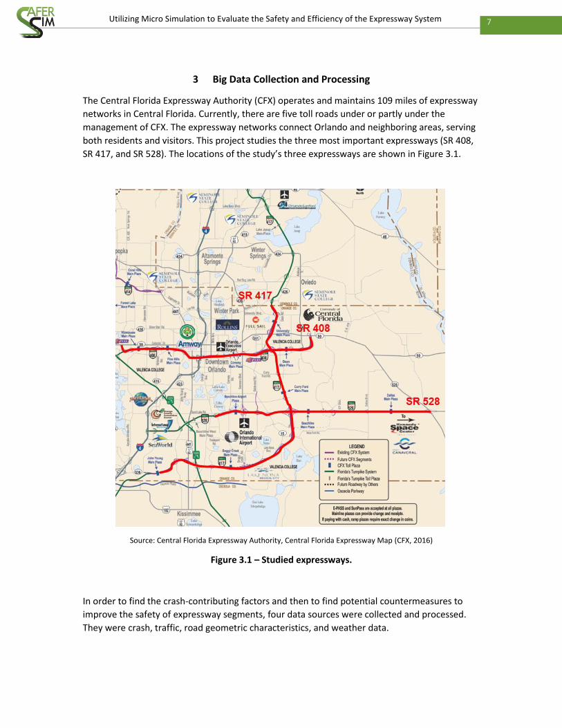
3 Big Data Collection and Processing
The Central Florida Expressway Authority (CFX) operates and maintains 109 miles of expressway
networks in Central Florida. Currently, there are five toll roads under or partly under the
management of CFX. The expressway networks connect Orlando and neighboring areas, serving
both residents and visitors. This project studies the three most important expressways (SR 408,
SR 417, and SR 528). The locations of the study’s three expressways are shown in Figure 3.1.
Source: Central Florida Expressway Authority, Central Florida Expressway Map (CFX, 2016)
Figure 3.1 – Studied expressways.
In order to find the crash-contributing factors and then to find potential countermeasures to
improve the safety of expressway segments, four data sources were collected and processed.
They were crash, traffic, road geometric characteristics, and weather data.
8 Utilizing Micro Simulation to Evaluate the Safety and Efficiency of the Expressway System
3.1 Crash Data
In Florida, crashes are recorded in two formats of crash reports, namely the short form and the
long form. Long-form crash reports are designed to keep records of more severe crashes,
especially those involving injuries or fatalities. Short-form crash reports are mostly used for
property-damage-only crashes. The Signal Four Analytics (S4A) data served as the crash data
source of this project. One issue with the S4A database is that for the crashes that occurred in
early years (e.g., early 2000s), the short-form crash reports were not complete. After June 2012,
S4A has the complete crash data from both types of reports for all of Florida. This research is
based on the data after July 2013; thus, there is no issue with the crash data.
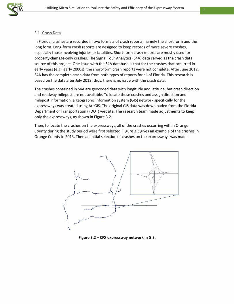
The crashes contained in S4A are geocoded data with longitude and latitude, but crash direction
and roadway milepost are not available. To locate these crashes and assign direction and
milepost information, a geographic information system (GIS) network specifically for the
expressways was created using ArcGIS. The original GIS data was downloaded from the Florida
Department of Transportation (FDOT) website. The research team made adjustments to keep
only the expressways, as shown in Figure 3.2.
Then, to locate the crashes on the expressways, all of the crashes occurring within Orange
County during the study period were first selected. Figure 3.3 gives an example of the crashes in
Orange County in 2013. Then an initial selection of crashes on the expressways was made.
Figure 3.2 – CFX expressway network in GIS.

9 Utilizing Micro Simulation to Evaluate the Safety and Efficiency of the Expressway System
Figure 3.3 – Total crashes in Orange County in 2013.
In the crash report, there is one column indicating the crash street based on which expressways
a crash was collected. However, the naming of the expressways is not consistent. As a solution,
several key words that could be used for the same expressway were extracted using the
structured query language (SQL) technique as shown in Table 3.1. The “%” means any string of
zero or more characters, and “_” means any single character within the string in SQL.
Table 3.1 – Key words used for expressway crash selection.
Expressway Key Words
SR 408 “%408%”, “%E-W%”, “%E/W%”, “%EAST_WEST%”, “EW %”, “%EASTWEST%”
SR 417 “%417%”, “%CENTRAL_FL%”, “GREENEWAY”
SR 528 “%528%”, “%BEELINE%”, “BEACHLINE”
Using these criteria, the initial selection was made as displayed in Figure 3.4. As can be seen in
Figure 3.4, the majority of the crashes after the initial selection are located on the CFX
expressway systems. A few of the crashes that are not related to the expressways were also
included because they share the same key words that are used to filter the expressway crashes.
In addition, some crashes on the expressways occurred on the segments that are not operated
by CFX. These crashes would also not be included in further analysis.

10 Utilizing Micro Simulation to Evaluate the Safety and Efficiency of the Expressway System
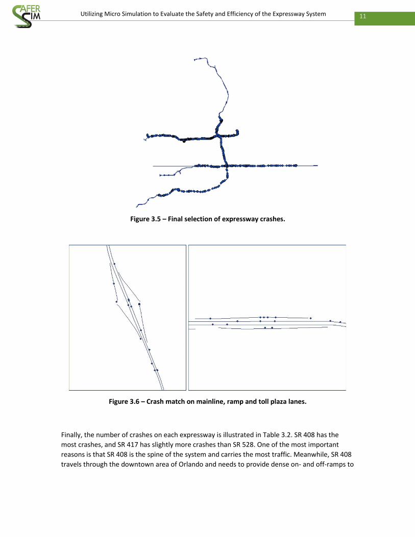
Therefore, a final selection of the crashes that happened on the studied expressways was
conducted by deleting the unrelated crash points in ArcGIS. The results of the final selection are
illustrated in Figure 3.5. In this figure, the crashes not related to expressways and those crashes
not occurring on segments operated by CFX have been excluded. In the final crash data, crashes
on the mainline, ramps, and toll plaza cash lanes on the segments managed by CFX are selected.
Figure 3.6 shows the detail about how these crashes are assigned. Both crash direction and
mileposts are assigned to the crashes using ArcGIS.
Figure 3.4 – Initial selection of expressway crashes
11 Utilizing Micro Simulation to Evaluate the Safety and Efficiency of the Expressway System
Figure 3.5 – Final selection of expressway crashes.
Figure 3.6 – Crash match on mainline, ramp and toll plaza lanes.
Finally, the number of crashes on each expressway is illustrated in Table 3.2. SR 408 has the
most crashes, and SR 417 has slightly more crashes than SR 528. One of the most important
reasons is that SR 408 is the spine of the system and carries the most traffic. Meanwhile, SR 408
travels through the downtown area of Orlando and needs to provide dense on- and off-ramps to
12 Utilizing Micro Simulation to Evaluate the Safety and Efficiency of the Expressway System
facilitate downtown traffic. Hence, the spacing between ramps sometimes is limited, and too-
short spacing increases crash potential (Ray et al., 2011).
Table 3.2 – Crash number of expressways.
Route Length
(mi)
Year Average Crash/mi
2013 2014 2015
SR 408 21.4 700 761 945 758 35.4
SR 417 31.5 355 476 567 442 14.0
SR 528 22.4 313 379 419 347 15.5
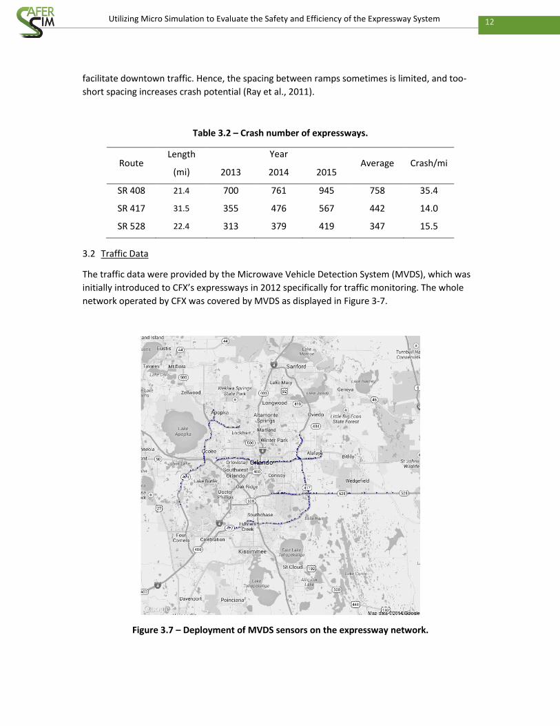
3.2 Traffic Data
The traffic data were provided by the Microwave Vehicle Detection System (MVDS), which was
initially introduced to CFX’s expressways in 2012 specifically for traffic monitoring. The whole
network operated by CFX was covered by MVDS as displayed in Figure 3-7.
Figure 3.7 – Deployment of MVDS sensors on the expressway network.

13 Utilizing Micro Simulation to Evaluate the Safety and Efficiency of the Expressway System
For the purpose of this project, MVDS data have been collected since July 2013. MVDS detectors
do not identify individual vehicles. They return aggregated traffic flow parameters for each lane
of each section, where the MVDS detector is installed, at one-minute intervals. The traffic
parameters include traffic volume, time mean speed, lane occupancy, and traffic volume by
vehicle length. Four types of vehicles were defined by their lengths:
Type 1: vehicles 0 to 10 feet in length
Type 2: vehicles 10 to 24 feet in length
Type 3: vehicles 24 to 54 feet in length
Type 4: vehicles over 54 feet in length
Additional information on traffic data from MVDS detectors includes the timestamp when the
sensor is polled. It was mentioned earlier that the sensors are polled every one minute. Also,
unique sensor identifiers and lane identifiers are contained within the data. The sensor identifier
consists of the roadway (i.e., SR 408, SR 417, or SR 528), milepost, and direction. The lanes are
counted from the roadway medium to the outside lane. The lanes fall into four categories:
Mainline, Ramp, Mainline TP Express, and Mainline TP Cash. Mainline TP Expressway indicates
express lanes at mainline toll plazas; vehicles equipped with tags do not need to slow down on
these lanes when they pass the toll plazas. Mainline TP Cash means toll booths at mainline toll
plazas; vehicles need to stop and pay tolls. On the expressways, these two types of lanes are
physically separated. Table 3.3 gives an example of the lane types and numbers at each MVDS
detection on eastbound SR 408. The detector information for other roadways can be found in
Appendix A.

14 Utilizing Micro Simulation to Evaluate the Safety and Efficiency of the Expressway System
Table 3.3 – SR 408 eastbound MVDS system and lane configuration.
Eastbound Number of lanes Eastbound Number of lanes
ID Milepost Mainline (w/ TP
Express) TP
Cash Ramp ID Milepost
Mainline (w/ TP Express)
TP Cash
Ramp
1 1.2 2 30 11.5 5 1
2 1.4 2 31 12.1 5
3 1.7 2 2 32 12.5 5 1
4 2.2 3 1 33 12.9 5 2
5 2.4 3 1 34 13.3 5 2
6 2.7 3 2 35 13.7 3 3
7 3.2 2 1 36 14.2 3 2
8 3.6 2 1 37 14.5 4
9 4.3 3 1 38 14.7 4 2
10 4.6 4 39 15 5
11 4.9 3 1 40 15.7 4 2
12 5.3 3 1 41 15.8 4 1
13 6 3 2 1 42 16.1 4 1
14 6.4 3 1 43 16.5 5
15 6.8 3 44 17.3 3 3
16 7 3 1 45 17.7 2 1
17 7.4 3 46 18 2 1
18 7.6 3 1 47 18.4 2 1
19 8 3 1 48 18.8 2 1
20 8.4 3 1 49 19 2 2
21 8.9 3 1 50 19.4 2 1
22 9.2 3 1 51 19.5 2 1
23 9.4 4 1 52 20.1 2 1
24 9.6 3 1 53 20.3 2
25 9.7 1 54 20.8 2 1
26 10.3 3 1 55 21.8 2
27 10.6 4 1 56 22.3 2 2
28 10.8 5 1 57 22.7 2
29 11.2 5 1

15 Utilizing Micro Simulation to Evaluate the Safety and Efficiency of the Expressway System
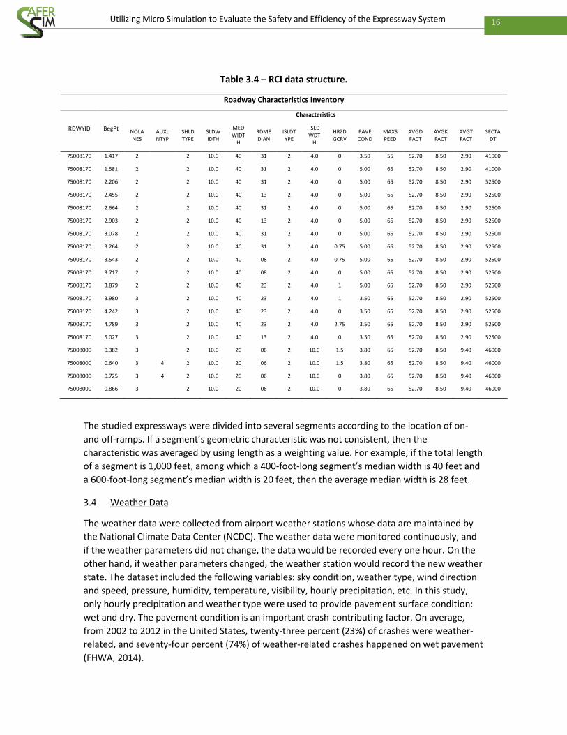
3.3 Road Geometric Characteristics Data
Roadway geometry has a significant impact on traffic operation and safety. The FDOT maintains
the Road Characteristics Inventory (RCI) database, which has roadway geometry and other
relevant information. The RCI database has hundreds of road characteristic variables. Only the
most relevant geometric variables were chosen for the data preparation. In sum, 15 variables
were selected: number of lanes, auxiliary lane type, shoulder type, shoulder width, median
width, median type, inside shoulder type, inside shoulder width, horizontal degree of curvature,
pavement condition, maximum speed limit, D factor, K factor, truck percentage, and section
ADT. Table 3.4 gives an example of the RCI data.
16 Utilizing Micro Simulation to Evaluate the Safety and Efficiency of the Expressway System
Table 3.4 – RCI data structure.
Roadway Characteristics Inventory
RDWYID BegPt
Characteristics
NOLANES
AUXLNTYP
SHLDTYPE
SLDWIDTH
MEDWIDT
H
RDMEDIAN
ISLDTYPE
ISLDWDT
H
HRZDGCRV
PAVECOND
MAXSPEED
AVGDFACT
AVGKFACT
AVGTFACT
SECTADT
75008170 1.417 2 2 10.0 40 31 2 4.0 0 3.50 55 52.70 8.50 2.90 41000
75008170 1.581 2 2 10.0 40 31 2 4.0 0 5.00 65 52.70 8.50 2.90 41000
75008170 2.206 2 2 10.0 40 31 2 4.0 0 5.00 65 52.70 8.50 2.90 52500
75008170 2.455 2 2 10.0 40 13 2 4.0 0 5.00 65 52.70 8.50 2.90 52500
75008170 2.664 2 2 10.0 40 31 2 4.0 0 5.00 65 52.70 8.50 2.90 52500
75008170 2.903 2 2 10.0 40 13 2 4.0 0 5.00 65 52.70 8.50 2.90 52500
75008170 3.078 2 2 10.0 40 31 2 4.0 0 5.00 65 52.70 8.50 2.90 52500
75008170 3.264 2 2 10.0 40 31 2 4.0 0.75 5.00 65 52.70 8.50 2.90 52500
75008170 3.543 2 2 10.0 40 08 2 4.0 0.75 5.00 65 52.70 8.50 2.90 52500
75008170 3.717 2 2 10.0 40 08 2 4.0 0 5.00 65 52.70 8.50 2.90 52500
75008170 3.879 2 2 10.0 40 23 2 4.0 1 5.00 65 52.70 8.50 2.90 52500
75008170 3.980 3 2 10.0 40 23 2 4.0 1 3.50 65 52.70 8.50 2.90 52500
75008170 4.242 3 2 10.0 40 23 2 4.0 0 3.50 65 52.70 8.50 2.90 52500
75008170 4.789 3 2 10.0 40 23 2 4.0 2.75 3.50 65 52.70 8.50 2.90 52500
75008170 5.027 3 2 10.0 40 13 2 4.0 0 3.50 65 52.70 8.50 2.90 52500
75008000 0.382 3 2 10.0 20 06 2 10.0 1.5 3.80 65 52.70 8.50 9.40 46000
75008000 0.640 3 4 2 10.0 20 06 2 10.0 1.5 3.80 65 52.70 8.50 9.40 46000
75008000 0.725 3 4 2 10.0 20 06 2 10.0 0 3.80 65 52.70 8.50 9.40 46000
75008000 0.866 3 2 10.0 20 06 2 10.0 0 3.80 65 52.70 8.50 9.40 46000
The studied expressways were divided into several segments according to the location of on-
and off-ramps. If a segment’s geometric characteristic was not consistent, then the
characteristic was averaged by using length as a weighting value. For example, if the total length
of a segment is 1,000 feet, among which a 400-foot-long segment’s median width is 40 feet and
a 600-foot-long segment’s median width is 20 feet, then the average median width is 28 feet.
3.4 Weather Data
The weather data were collected from airport weather stations whose data are maintained by
the National Climate Data Center (NCDC). The weather data were monitored continuously, and
if the weather parameters did not change, the data would be recorded every one hour. On the
other hand, if weather parameters changed, the weather station would record the new weather
state. The dataset included the following variables: sky condition, weather type, wind direction
and speed, pressure, humidity, temperature, visibility, hourly precipitation, etc. In this study,
only hourly precipitation and weather type were used to provide pavement surface condition:
wet and dry. The pavement condition is an important crash-contributing factor. On average,
from 2002 to 2012 in the United States, twenty-three percent (23%) of crashes were weather-
related, and seventy-four percent (74%) of weather-related crashes happened on wet pavement
(FHWA, 2014).

17 Utilizing Micro Simulation to Evaluate the Safety and Efficiency of the Expressway System
At a timestamp, if the hourly precipitation was higher than zero, or weather type contained TS
(thunderstorm), RA (rain), or DZ (drizzle), it meant rainy weather condition. Then, it was
assumed that the roadway surface condition was wet in the following one hour of this
timestamp (Wang et al., 2015b).

18 Utilizing Micro Simulation to Evaluate the Safety and Efficiency of the Expressway System
4 Safety Analysis of Expressway System
4.1 Introduction
In order to understand crash causes, a significant number of studies have linked traffic safety
with crash-contributing factors such as traffic and geometry. Among these research efforts, the
majority have been based on highly aggregated traffic data, i.e., AADT and ADT. However, an
expressway with high traffic flow during peak hours would have a different crash potential than
an expressway with the same ADT but a traffic flow that is evenly spread out throughout the day
(Mensah & Hauer, 1998). Meanwhile, the crash occurrence should be more related to the
prevailing conditions prior to the crash than to ADT. Hence, in addition to ADT-based safety
studies, this project explored crash more closely through hourly crash studies based on AHT and
through real-time crash studies based on microscopic traffic at five-minute intervals.
Hourly crash studies average one or several hours’ worth of traffic data over a long time and
also aggregate crash frequencies in the corresponding hour(s); for example, the AHT from 8:00
A.M. to 9:00 A.M. in 2015, and the number of corresponding crashes that occurred from 8:00
A.M. to 9:00 A.M. in 2015. Then, the study applies models to find the statistical relationship
between hourly crash frequency and hourly traffic flow characteristics along with geometric
factors (Lord et al., 2005). If an expressway’s hourly traffic does not change much during the
day, an hourly crash study would be similar to a crash study based on ADT. Nevertheless,
expressways generally have peak and non-peak traffic hours, so an AHT-based crash study might
outperform an ADT-based crash study.
Real-time crash analyses use each crash as an event, unlike ADT- and AHT-based studies, which
use a segment as a unit for frequencies. In a real-time crash analysis, the condition that occurred
just before a crash, such as a traffic situation, is considered to be among the contributing factors
that led to the crash and is defined as a crash event. On the other hand, if no crash happens, the
condition is defined as non-crash event. By comparing crash to non-crash events, crash
precursors that are relatively more “crash prone” than others can be identified (Lee et al., 2002;
Abdel-Aty et al., 2005). Real-time safety analyses have been broadly used to predict crash
hazards in real time and to test the safety impact of ATM, such as RM and VSL (Lee et al., 2006;
Yu & Abdel-Aty, 2014).
All three of the above-mentioned types of traffic safety analyses, especially those based on ADT
and microscopic traffic at five-minute intervals, have already been widely studied by previous
researchers. However, almost all of the previous studies focused only on one of them. There is a
need to compare these three types of safety analyses to identify which one is able to provide
better crash estimation. The objectives of this chapter are as follows: (1) to identify the different
approaches to analyzing safety at the segment level; (2) to evaluate the stability of the three
types of safety analyses in identifying the important contributing factors and their ability to use
the identified variables to predict safety conditions; (3) to compare the performance of the
different modeling approaches; and (4) to evaluate the safety of the different segment types
(i.e., basic, weaving, merge, and diverge).

19 Utilizing Micro Simulation to Evaluate the Safety and Efficiency of the Expressway System
4.2 Data Preparation
The studied segments were from the three studied expressways in Central Florida: SR 408, 417,
and 528. The study period was from July 2013 to December 2015, and April 2014 was excluded
because traffic data were not available during that month. This study classified segments into
four types according to HCM (2010): merge segments, diverge segments, weaving segments,
and basic segments. The layouts of merge, diverge, and weaving segments are illustrated in
Figure 4.1. Basic segments are other expressway segments that are not among the three types
of segments listed in Figure 4.1.
Figure 4.1 – Different segment types.
In total, the three studied expressways have 339 segments. However, not all of these 339
segments were explored. Three sorts of segments were excluded from further analysis, they
were toll-plaza-related segments (i.e., the toll plaza and its upstream and downstream
segments), segments whose length was less than 500 feet, and segments whose traffic data
were not available. The lane configurations of toll-plaza-related segments are very different
from other segments; hence, the safety of a toll plaza should not be treated as the same as the
other segments and put in the same safety study. For the segments whose length was less than
500 feet, some crashes were on the boundaries of two segments and were randomly assigned
to one of the two segments. If a segment is too short, the crash frequency on this segment is
usually very low; hence, the random assignment of the crashes on boundaries might have a
significant impact on crash frequency results. For example, if the length of a studied segment is
3,000 feet, and five crashes happened in this segment. Adding one crash that happened on the
boundary to the studied segment produces six crashes in total. The number of six crashes is just
20% different from the number of five crashes, which is the condition that this boundary crash is
assigned to a neighbor segment but not the studied segment. On the other hand, if the length is
400 feet, and one crash happened in this segment. Adding one crash on the boundary to the
studied segment produces two crashes in total. The number of two crashes is 100% different

20 Utilizing Micro Simulation to Evaluate the Safety and Efficiency of the Expressway System
from the number of one crashes, which is the condition that this boundary crash is assigned to a
neighbor segment.
Finally, 247 segments were chosen as the study subject, among which 45 were merge segments,
48 were diverge segments, 25 were weaving segments, and 129 were basic segments. The
geometric information of the studied segments was mainly obtained from RCI, including number
of lanes, speed limit, median width, inside shoulder width, and outside shoulder width. Segment
lengths were automatically created by ArcGIS Map. The descriptive analysis of the geometry of
studied segments is shown in Table 4.1.
Table 4.1 – Descriptive analysis of the geometric characteristic.
Variables Mean Std. Min. Max.
Segment length (feet) 3165.65 3396.09 619.08 27652.60
Median width (feet) 46.61 15.30 16 64
Number of lane (lane) 2.66 0.87 0 5
Speed limit (mph) 67.27 4.82 55 70
Inside shoulder width (feet) 7.29 3.56 4 24
Outside shoulder width (feet) 9.64 1.07 2 12
The raw traffic data were obtained from the MVDS, which collected traffic data, including
vehicle count, lane occupancy, and speed, for each lane at one-minute intervals. Additionally,
the detectors recognized the length of passing vehicles and categorized them under four groups.
The vehicle lengths of Groups 3 and 4 were greater than 24 feet; the vehicles in Group 3 and 4
were consider to be trucks, and the total volume of Groups 3 and 4 were used as trucks volume.
The traffic data were aggregated into three types: ADT, AHT, and microscopic traffic data at five-
minute intervals.
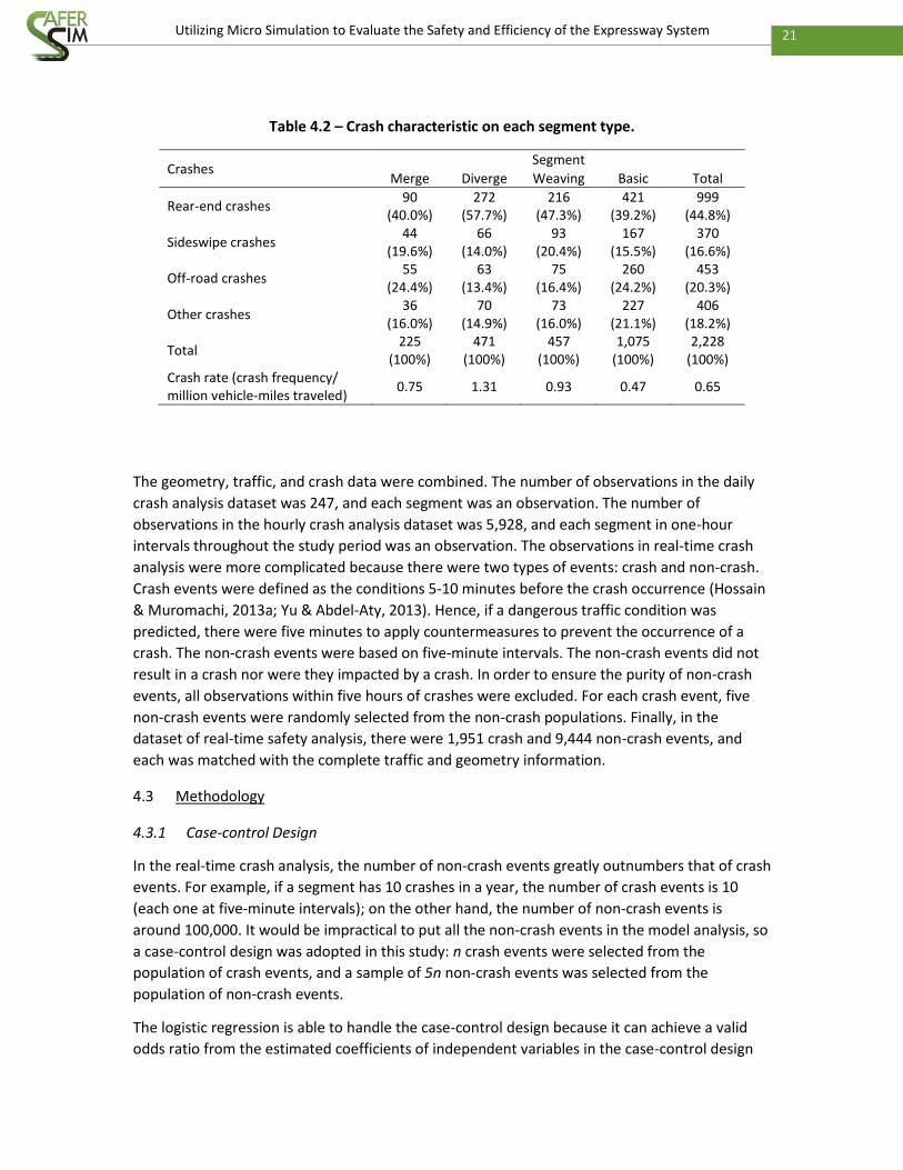
The crash data were from the S4A, which provided detailed crash information, such as crash
time, location, severity, and type. The crash characteristics for each segment type are illustrated
in Table 4.2. The crash rate of the diverge segment was 1.31, and percentage of rear-end
crashes on the diverge segment was 57.7%, which was much higher than that of other
segments. An off-ramp vehicle on the diverge segment might decelerate dramatically due to the
much lower speed limit on off-ramps than on mainlines. If its following vehicle does not
decrease speed in time, a rear-end crash might happen. The crash rate of weaving segments was
as high as 0.93 because vehicles merge, diverge, and weave in a limited space (Wang et al.,
2015a).
21 Utilizing Micro Simulation to Evaluate the Safety and Efficiency of the Expressway System
Table 4.2 – Crash characteristic on each segment type.
Crashes Segment
Merge Diverge Weaving Basic Total
Rear-end crashes 90
(40.0%) 272
(57.7%) 216
(47.3%) 421
(39.2%) 999
(44.8%)
Sideswipe crashes 44
(19.6%) 66
(14.0%) 93
(20.4%) 167
(15.5%) 370
(16.6%)
Off-road crashes 55
(24.4%) 63
(13.4%) 75
(16.4%) 260
(24.2%) 453
(20.3%)
Other crashes 36
(16.0%) 70
(14.9%) 73
(16.0%) 227
(21.1%) 406
(18.2%)
Total 225
(100%) 471
(100%) 457
(100%) 1,075
(100%) 2,228
(100%) Crash rate (crash frequency/ million vehicle-miles traveled)
0.75 1.31 0.93 0.47 0.65
The geometry, traffic, and crash data were combined. The number of observations in the daily
crash analysis dataset was 247, and each segment was an observation. The number of
observations in the hourly crash analysis dataset was 5,928, and each segment in one-hour
intervals throughout the study period was an observation. The observations in real-time crash
analysis were more complicated because there were two types of events: crash and non-crash.
Crash events were defined as the conditions 5-10 minutes before the crash occurrence (Hossain
& Muromachi, 2013a; Yu & Abdel-Aty, 2013). Hence, if a dangerous traffic condition was
predicted, there were five minutes to apply countermeasures to prevent the occurrence of a
crash. The non-crash events were based on five-minute intervals. The non-crash events did not
result in a crash nor were they impacted by a crash. In order to ensure the purity of non-crash
events, all observations within five hours of crashes were excluded. For each crash event, five
non-crash events were randomly selected from the non-crash populations. Finally, in the
dataset of real-time safety analysis, there were 1,951 crash and 9,444 non-crash events, and
each was matched with the complete traffic and geometry information.
4.3 Methodology
4.3.1 Case-control Design
In the real-time crash analysis, the number of non-crash events greatly outnumbers that of crash
events. For example, if a segment has 10 crashes in a year, the number of crash events is 10
(each one at five-minute intervals); on the other hand, the number of non-crash events is
around 100,000. It would be impractical to put all the non-crash events in the model analysis, so
a case-control design was adopted in this study: n crash events were selected from the
population of crash events, and a sample of 5n non-crash events was selected from the
population of non-crash events.
The logistic regression is able to handle the case-control design because it can achieve a valid
odds ratio from the estimated coefficients of independent variables in the case-control design

22 Utilizing Micro Simulation to Evaluate the Safety and Efficiency of the Expressway System
(Hosmer et al., 2013). Suppose A is a crash event, and B stands for an observation in the dataset
of the real-time crash analysis that is selected from the whole population; the possibility that a
selected observation is a crash event is p(A|B), which is calculated as follows:
( ) ( | )( | )
( ) ( | ) ( ) ( | )
p A p B Ap A B
p A p B A p A p B A
(4.1)
where A means an observation is not a crash event. From Equation (4.1), the ratio is as follows:
( | ) ( ) ( | )
1 ( | ) ( ) ( | )
p A B p A p B A
p A B p A p B A
(4.2)
Suppose that ( | )p B A is the percentage of crash events that have been sampled (p1) and
( | )p B A is the percentage of non-crash events that have been sampled (p2). Equation (4.2)
could be written as follows:
1
2
( | ) ( )
1 ( | ) 1 ( )
pp A B p A
p A B p A p
(4.3)
In a logistic regression model without case-control design, the crash ratio is estimated using the
following equation:
0 1
( )log( )
1 ( )
R
r rr
p Ax
p A
(4.4)
where 0 is the threshold, and r is the estimated coefficient of the rth explanatory variables (
rx ). Putting Equation (4.4) into Equation (4.3), the crash ratio under case-control design is as
follows:
'10 01 1
2
( | )log( ) ln( )
1 ( | )
R R
r r r rr r
pp A Bx x
p A B p
(4.5)
By comparing Equations (4.4) and (4.5), it can be found that the only difference between the
logarithm of crash ratio under case-control design and that under non-case-control design is the
intercept. Hence, in order to obtain the true intercept 0 , 1 2ln( / )p p should be subtracted
from 0
' , which is estimated under case-control design. Both p1 and p2 are available, so the true
crash ratio and then the true crash likelihood for each five-minute interval are ready to be
calculated if the real-time crash analysis model is obtained.
4.3.2 Crash Prediction Models
In the hourly crash analysis, each segment has 24 observations in total. In the real-time safety
analysis, a segment has several crash and non-crash events. The observations on the same
segment might be correlated; meanwhile, a segment might have different crash potentials
compared with other segments since there might be some uncaptured characteristics of each
segment. Multilevel models were used to handle the two issues (Gelman & Hill, 2006).

23 Utilizing Micro Simulation to Evaluate the Safety and Efficiency of the Expressway System
For ADT-based total crash frequency estimation, a Bayesian Poisson-lognormal model was used.
The Poisson-lognormal model has been widely used in crash frequency analyses to handle the
over-dispersion problem (Lord & Mannering, 2010). For the AHT-based crash frequency
prediction, a Bayesian multilevel Poisson-lognormal model was used. It was assumed that the
observed crash frequency at time interval t on segment i (yti) had a Poisson distribution, whose
mean was the expected crash frequency (𝛌ti):
~ ( )ti tiy Poisson (4.6)
Individual level:
0 1log( )
R
ti i r rti tirx
(4.7)
Segment level:
0 2~ ( ,1/ )i iNormal g (4.8)
0 1
Q
i q q iqg w
(4.9)
where r is the regression coefficient of the rth individual-level independent parameter ( rx ), R
is the total number of individual-level independent parameters, and ti is the residual and was
set to follow a normal distribution. 0i is the intercept at the individual-level model; it was
assumed to vary across segments and is conditioned on the geometric factor ig . 0 is the
intercept of segment level, q is the coefficient of the qth segment-level variable ( qw ), Q is the
total number of segment-level independent parameters, i is the unexplained segment-level
errors and is normally distributed with a mean of 0 and a deviation of 3 . All 0 , q , and r
were specified to be vague normal distributed priors: normal (0, 106). 1 , 2 , and 3 were
specified to have gamma prior: gamma (0.001,0.001).
For the five-minute-based safety analysis under case-control design, a Bayesian multilevel
logistic regression model was used. An observation at time interval t on segment i (yti) has a
binary outcome, crash (yti=1) and non-crash (yti=0); their possibilities are pti (yti=1) and 1-pti
(yti=0), respectively:
~ ( )ti tiy Bernoulli p (4.10)
Individual level:
0 1log( )
1
Rtii r rtir
ti
px
p
(4.11)
Segment level:

24 Utilizing Micro Simulation to Evaluate the Safety and Efficiency of the Expressway System
0 1~ ( ,1/ )i iNormal g (4.12)
0 1
Q
i q q iqg w
(4.13)
The variable definition of the Bayesian multilevel logistic regression model is similar to the
Bayesian multilevel Poisson-lognormal model.
All three models, the Bayesian Poisson-lognormal, the Bayesian multilevel Poisson-lognormal,
and the Bayesian multilevel logistic regression, were estimated in WinBUGS. For each model,
three chains of 10,000 iterations were set up, and only the second half of the iterations were
used in the final analysis to exclude the impact of the initial values (Gelman et al., 2014). For all
parameters in the three Bayesian models, the trace plots of three chains appeared to have been
stabilized, and the three chains were overlapping each other. This indicated that models were
converged.
4.3.3 Model Comparison
After the three models were estimated, the total and hourly crash frequencies for each segment
were calculated, and the true real-time crash likelihoods at five-minute intervals for each
segment were also computed. Then, the predicted crash frequency and crash likelihoods were
used to obtain the crash condition at three different levels: total, hourly, and five-minute
intervals. To be more specific (Figure 4.2):
1. The predicted total crash frequency (based on ADT) was divided by 24 hours to obtain
the hourly crash count and then divided by the number of five-minute intervals in the
study period (884 days × 24 hours ×12 intervals) to obtain crash likelihoods at five-
minute intervals;
2. The 24 hourly crash frequencies on each segment were all aggregated together to
provide the total crash frequency of that segment, and they were also divided by the
number of five-minute intervals in one-hour intervals throughout the study period (884
days × 12 intervals);
3. The conditional crash likelihoods at five-minute intervals under case-control design were
first calculated and transferred to actual crash likelihood. Then, the actual crash
likelihoods were aggregated into total crash frequencies and hourly crash frequencies.

25 Utilizing Micro Simulation to Evaluate the Safety and Efficiency of the Expressway System
Figure 4.2 – Model results transformation.
After transformation, there were three estimated crash conditions, i.e., ADT-based, AHT-based,
and five-minute-based, for each time level. Then, the estimated crash conditions were
compared with the field crash conditions. For crash frequency comparison, mean absolute
deviation (MAD) was used to estimate the consistency between estimated and true crash
conditions,
MAD=∑ |𝑦𝑖−��𝑖|𝑛
𝑖=1
𝑛 (4.14)
26 Utilizing Micro Simulation to Evaluate the Safety and Efficiency of the Expressway System
where n is the number of total observations, 𝑦𝑖 is the field crash frequency of the ith observation,
and ��𝑖 is the predicted crash frequency of the ith observation.
With respect to the crash risk at five-minute intervals, the measurement area under the receiver
operating characteristic (ROC) curve was adopted. The ROC is a standard for evaluating a
model’s ability to correctly assign an observation to the correct group (Hosmer et al., 2013). The
curve plots the possibility of detecting true crash events and the possibility of detecting false
crash events for an entire range of possible thresholds (from 0 to 1.0). The area under the ROC
curve ranges from 0.5 to 1.0. A higher value indicates a better ability to discriminate crash from
non-crash events.
One of the most important targets of real-time crash analysis is the identification of hazard
conditions for ATM, such as RM. The segments and time period with high crash potentials are of
great interest for ATM (Abdel-Aty et al., 2007). On the other hand, if a segment does not have
any crashes over a very long period of time, there is no need to install ATM or to identify high
crash risk. Hence, distinguishing crash events for the segments with high historical crash
frequencies is better than doing so for all segments. For any hour-long interval (for example,
7:00 A.M. to 8:00 A.M.) throughout the study period (884 days), if a segment had more than one
crash in that interval, this segment in this hour period was chosen to provide data at five-minute
intervals for model comparison. In total, 1,065 crash events were filtered, and 5,325 non-crash
events were randomly selected for ROC calculation.
4.4 Model Estimation and Comparison
4.4.1 Crash Prediction Model
Before model estimation, each independent variable alone was put into models to find out
whether it had significant impact on safety at an 85% confidence interval. Then, after
insignificant variables were deleted, Pearson correlation tests were conducted to evaluate the
correlation between variables. When the correlation between a variable and volume was higher
than 0.4, then this variable was excluded in the model building; when both of the variables were
not volume, and their correlation coefficient was higher than 0.4, the variable that could provide
a lower deviance information criterion (DIC) was chosen. The models’ results are presented in
Table 4.3.
Overall, the significant variables in the three models are similar. Four out of eight significant
variables were common, and all common variables have the same signs. All significant variables
in the ADT-based crash prediction model were included in the AHT-based crash prediction
model. Meanwhile, except for one variable (speed), all significant variables in the five-minute-
based safety analysis model could be found in the AHT-based crash prediction model. This
indicates that the crash-contributing factors discovered by the three models were comparable.

27 Utilizing Micro Simulation to Evaluate the Safety and Efficiency of the Expressway System
Table 4.3 – Crash prediction model.
Definition ADT-based AHT-based 5-minute-based
Mean Std.# 95% CI Mean Std. 95% CI Mean Std. 95% CI
Intercept -0.74 2.09 (-5.29,3.66) -4.84 0.94 (-6.66,-3.01) -3.25 0.35 (-3.92, -2.58)
Log (volume per lane) 0.57 0.17 (0.25,0.92) 0.72 0.04 (0.65,0.79) 0.80 0.05 (0.71, 0.89)
Speed limit (mph) -0.06 0.01 (-0.07,-0.04) -0.04 0.01 (-0.06,-0.01) --* --* --*
Speed (mph) --* --* --* --* --* --* -0.05 0.00 (-0.06,-0.04)
Truck percentage --* --* --* 1.54 0.54 (0.48,2.60) 2.57 0.33 (1.90,3.20)
Number of lanes (lane) 0.17 0.07 (0.04,0.30) 0.22 0.06 (0.10,0.34) 0.27 0.06 (0.15,0.38)
Segment length (103 ft) 0.14 0.01 (0.11,0.16) 0.15 0.01 (0.12,0.17) 0.16 0.01 (0.13,0.19)
Weaving segment 0.57 0.17 (0.24,0.90) 0.70 0.16 (0.39,1.01) 0.34 0.17 (0.03,0.68)
Diverge segment --* --* --* 0.42 0.12 (0.18,0.65) --* --* --*
std. of Ɛi N/A N/A N/A 0.43 0.20 (0.04,0.64) 0.23 0.18 (0.03,0.60)
DIC 1293.210 7712.350 5752.180
Training ROC N/A** N/A 0.813
Validation ROC N/A N/A 0.771
# Standard deviation
* Not significant
** Not available
The exposure variables, i.e., the logarithm of volume per lane, the number of lanes, and the
segment length, were found to have significantly positive impacts on crashes in all three models.
The higher the exposure variables, the higher the crash frequency and the higher the crash ratio.
In addition to exposure variables, other traffic and geometric factors were also found to be
significant. Speed had a negative impact on crash ratio in real time. High speed indicates that
the traffic condition is smooth and there is no congestion, so the crash potential is low. The
same negative relationship between speed and crashes has also been found by other
researchers (Hossain & Muromachi, 2013a). Speed limit was negatively related to crash
frequency. Segments with high speed limits are mainly in rural areas where there are fewer on-
and off-ramps; hence, the number of lane changes because of on- and off-ramps is lower.
Meanwhile, for the studied segments, the correlation coefficient between speed limit and
median width was 0.59 and was significant at the 5% confidence interval. The large median
width also enhanced the safety of segments (Park et al., 2016).
Truck percentage was not significant in the ADT-based crash prediction model. Truck percentage
varies significantly at different hours of day (Pahukula et al., 2015). However, the ADT-based
crash prediction model was not able to capture the variability and failed to link crash count with
trucks. On the other hand, truck percentage was positively significant in both the AHT-based
crash frequency and the five-minute-based crash analysis models. A higher truck percentage

28 Utilizing Micro Simulation to Evaluate the Safety and Efficiency of the Expressway System
results in a higher crash frequency and a higher crash ratio. The characteristics of passenger cars
and trucks are different; for example, trucks travel with a lower speed than passenger cars
(Johnson & Murray, 2010). A higher truck percentage implies more traffic turbulence and would
increase crash potential.
Weaving segments are more dangerous than other types of segments. A weaving segment is a
combination of a merge and a diverge segment. Hence, compared to other segments, weaving
segments have more complicated traffic since vehicles merge, diverge, and cross each other
over a short section (Wang et al., 2015a). Meanwhile, the high speed difference between
weaving and non-weaving traffic might also be a reason that weaving segments have higher
crash hazards (Pulugurtha & Bhatt, 2010). In the AHT-based crash prediction model, diverge
segments had an increased crash frequency. Vehicles traveling from mainlines to off-ramps
usually decelerate to adjust to the lower speed limit on off-ramps. If a vehicle decelerates
significantly and its following vehicle does not react in time, a rear-end crash might happen. In
this study, the crash characteristic confirms the interpretation. The rear-end crash percentage
for diverge segments was 57.7%, which is significantly higher than for merge segments (40.0%),
weaving segments (47.3%), and basic segments (39.2%).
With regard to the standard deviation of the segment-level error term, “std. of Ɛi”, it was
statistically significant at the 5% confidence interval for both AHT-based and five-minute-based
crash prediction models. It indicates that the between-segment variability was significant and
implies that the multilevel model structure was appropriate.
4.4.2 Model Comparison Results
After three crash prediction models were obtained, they were compared. The comparison
results are shown in Table 4.4.
Table 4.4 – Model comparison results.
To From predict models
MAD MAD ROC
total crash frequency
hourly crash frequency
5-minute crash likelihood
ADT-based model 1.060 0.473 0.599 AHT-based model 0.985 0.326 0.640 5-minute-based model 3.113 0.431 0.702
The results show that the AHT-based and five-minute-based model performed well in their own
areas: the AHT-based model was the best model for estimating hourly crash frequency, and the
5-minute-based model was the best for distinguishing crash from non-crash events. On the
other hand, the ADT-based model did not perform as well as the AHT-based model in predicting
total crash frequency. Meanwhile, the ADT-based model performed the worst in predicting
hourly crash frequency and crash likelihood at five-minute intervals. The result indicates that it
is not appropriate to assume that traffic conditions are not diverse throughout the day or to
suppose that the crash potential is evenly distributed.

29 Utilizing Micro Simulation to Evaluate the Safety and Efficiency of the Expressway System
The AHT-based crash prediction model performed the best in predicting total and hourly crash
frequency. The studied expressways are mainly used for commuting; they have morning and
evening traffic peak hours (see Figure 4.3). Volume is one of the most important crash-
contributing factors; therefore, the field crash frequency also had two peaks, which were
consistent with the traffic pattern. The hourly crash study was able to capture the traffic pattern
better than the crash study based on ADT; additionally, the AHT-based model is better than the
five-minute-based model because the aggregated hourly traffic largely excluded the impact of
temporal turbulence.
Figure 4.3 – Hourly volume and crash frequency.
The five-minute-based crash analysis model performed well in determining crash likelihood at
five-minute intervals by providing a higher ROC. The ADT and AHT are aggregated traffic
parameters; however, the occurrence of crashes could be attributed to temporal conditions. For
example, a segment has a crash because of unexpected heavy traffic over several minutes
during off-peak hours. The aggregated traffic factors might not be able to explain the occurrence
of this crash, whereas the real-time crash analysis can.
4.5 Summary
The traffic safety studies based on ADT, AHT, and traffic at five-minute intervals have been
widely and respectively explored by previous researchers. Nevertheless, there are not enough
studies, which compare these three types of traffic safety analyses. This study first built three
models: a Bayesian Poisson-lognormal model to estimate total crash frequency using ADT, a
Bayesian multilevel Poisson-lognormal model to predict hourly crash frequency using AHT, and a
Bayesian multilevel logistic regression model to estimate real-time crash risk under case-control
design using traffic at five-minute intervals. Then, the models were compared to find their
0
500
1000
1500
2000
2500
3000
0
0.2
0.4
0.6
0.8
1
0 2 4 6 8 10 12 14 16 18 20 22
Aver
age
Ho
url
y V
olu
me/
Seg
men
t
Cra
sh F
req
uen
cy/S
egm
ent
Hour
Volume and Crash Frequency
Field Hourly Crash Predicted Hourly Crash based on AHT
Predicted Hourly Crash based on ADT Hourly Average Volume
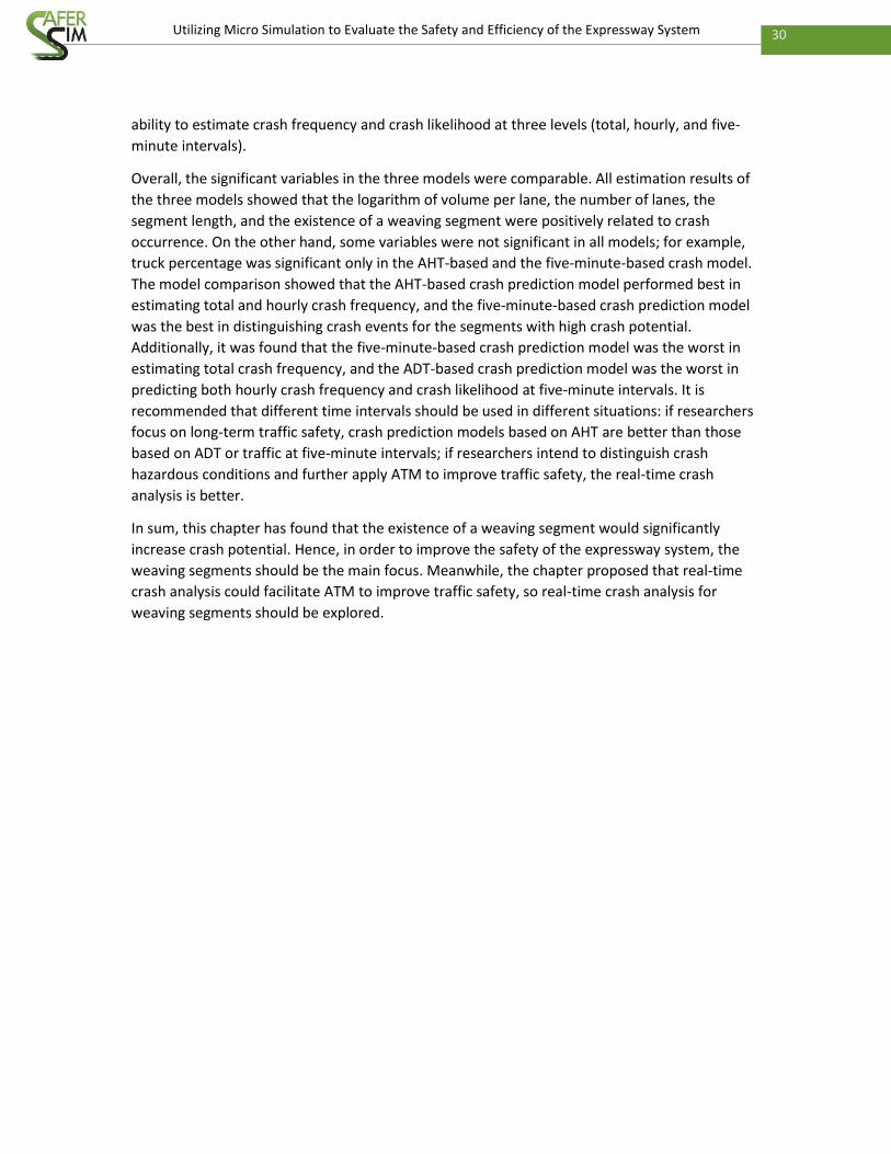
30 Utilizing Micro Simulation to Evaluate the Safety and Efficiency of the Expressway System
ability to estimate crash frequency and crash likelihood at three levels (total, hourly, and five-
minute intervals).
Overall, the significant variables in the three models were comparable. All estimation results of
the three models showed that the logarithm of volume per lane, the number of lanes, the
segment length, and the existence of a weaving segment were positively related to crash
occurrence. On the other hand, some variables were not significant in all models; for example,
truck percentage was significant only in the AHT-based and the five-minute-based crash model.
The model comparison showed that the AHT-based crash prediction model performed best in
estimating total and hourly crash frequency, and the five-minute-based crash prediction model
was the best in distinguishing crash events for the segments with high crash potential.
Additionally, it was found that the five-minute-based crash prediction model was the worst in
estimating total crash frequency, and the ADT-based crash prediction model was the worst in
predicting both hourly crash frequency and crash likelihood at five-minute intervals. It is
recommended that different time intervals should be used in different situations: if researchers
focus on long-term traffic safety, crash prediction models based on AHT are better than those
based on ADT or traffic at five-minute intervals; if researchers intend to distinguish crash
hazardous conditions and further apply ATM to improve traffic safety, the real-time crash
analysis is better.
In sum, this chapter has found that the existence of a weaving segment would significantly
increase crash potential. Hence, in order to improve the safety of the expressway system, the
weaving segments should be the main focus. Meanwhile, the chapter proposed that real-time
crash analysis could facilitate ATM to improve traffic safety, so real-time crash analysis for
weaving segments should be explored.

31 Utilizing Micro Simulation to Evaluate the Safety and Efficiency of the Expressway System
5 Real-time Safety Analysis for Weaving Segments
5.1 Introduction
In urban areas, the demand of exiting and entering expressway traffic is high. Hence, more on-
and off-ramps are needed than in rural areas. The dense on- and off-ramps might result in
limited spacing between them. When an on-ramp is closely followed by an off-ramp and the two
are connected by auxiliary lane(s), a weaving segment is formed. Weaving is generally defined as
the crossing of two or more traffic streams traveling in a same direction along a significant
length of highway without the aid of traffic devices (except for guide signs) (National Research
Council, 2010). Normally, there are three types of movement in weaving segments: mainline-to-
mainline, mainline-to-ramp, and ramp-to-mainline. There also might be some ramp-to-ramp
traffic; however, this type of traffic is not frequent since a traveler is not very likely to pay a toll
fee and just travel a short distance (normally less than 1 mile). Hence, ramp-to-ramp traffic is
not considered. The three types of main traffic movements are shown in Figure 5.1.
Figure 5.1 – Weaving segment traffic movements.
Traffic conditions in weaving segments are complicated because on-ramp and off-ramp vehicles
have to compete for lane-changing opportunities in a limited distance. Meanwhile, low-speed
entering vehicles need to accelerate in order to join mainline traffic, and exiting vehicles have to
decelerate in order to adjust to the lower speed limits of off-ramps. These frequent lane-
changing, acceleration, and deceleration maneuvers might result in an increased crash risk in
weaving segments. As for a congested weaving segment, these maneuvers might be more
intense, and the safety concerns of the congested weaving segment are more severe than other
segments.
The occurrence of crashes in weaving segments can bring about serious results. On-ramp
vehicles might not be able to get on expressways and may have to change their routes. Off-ramp
traffic may have difficulty getting off mainlines and may queue up on mainlines. Moreover, if
crashes cannot be cleared in time, the queue may block all traffic, both non-weaving and
weaving. Then the capacity and level of service of weaving segments will be reduced
significantly. Hence, understanding the crash mechanisms of weaving segments and finding
potential solutions to mitigate crash risks are significantly important.
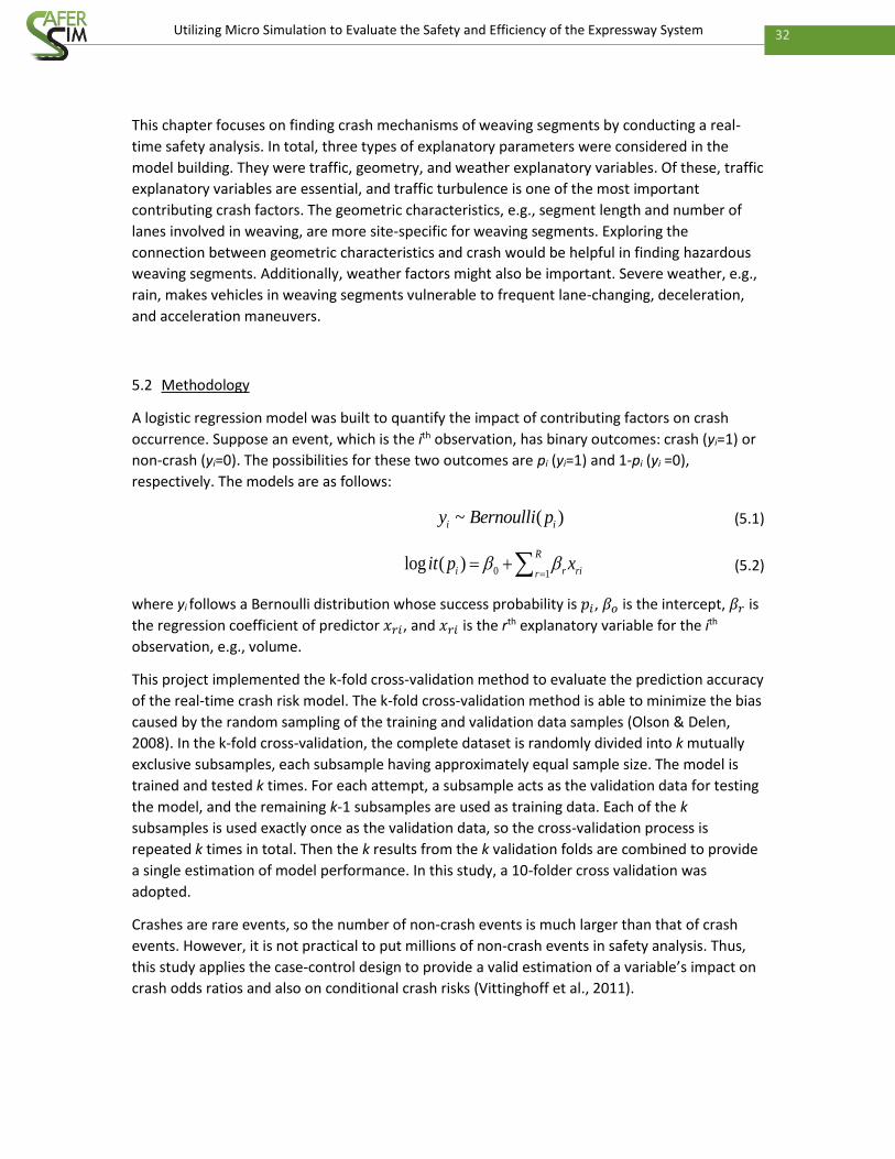
32 Utilizing Micro Simulation to Evaluate the Safety and Efficiency of the Expressway System
This chapter focuses on finding crash mechanisms of weaving segments by conducting a real-
time safety analysis. In total, three types of explanatory parameters were considered in the
model building. They were traffic, geometry, and weather explanatory variables. Of these, traffic
explanatory variables are essential, and traffic turbulence is one of the most important
contributing crash factors. The geometric characteristics, e.g., segment length and number of
lanes involved in weaving, are more site-specific for weaving segments. Exploring the
connection between geometric characteristics and crash would be helpful in finding hazardous
weaving segments. Additionally, weather factors might also be important. Severe weather, e.g.,
rain, makes vehicles in weaving segments vulnerable to frequent lane-changing, deceleration,
and acceleration maneuvers.
5.2 Methodology
A logistic regression model was built to quantify the impact of contributing factors on crash
occurrence. Suppose an event, which is the ith observation, has binary outcomes: crash (yi=1) or
non-crash (yi=0). The possibilities for these two outcomes are pi (yi=1) and 1-pi (yi =0),
respectively. The models are as follows:
~ ( )i iy Bernoulli p (5.1)
0 1log ( )
R
i r ririt p x
(5.2)
where yi follows a Bernoulli distribution whose success probability is 𝑝𝑖, 𝛽𝑜 is the intercept, 𝛽𝑟 is
the regression coefficient of predictor 𝑥𝑟𝑖, and 𝑥𝑟𝑖 is the rth explanatory variable for the ith
observation, e.g., volume.
This project implemented the k-fold cross-validation method to evaluate the prediction accuracy
of the real-time crash risk model. The k-fold cross-validation method is able to minimize the bias
caused by the random sampling of the training and validation data samples (Olson & Delen,
2008). In the k-fold cross-validation, the complete dataset is randomly divided into k mutually
exclusive subsamples, each subsample having approximately equal sample size. The model is
trained and tested k times. For each attempt, a subsample acts as the validation data for testing
the model, and the remaining k-1 subsamples are used as training data. Each of the k
subsamples is used exactly once as the validation data, so the cross-validation process is
repeated k times in total. Then the k results from the k validation folds are combined to provide
a single estimation of model performance. In this study, a 10-folder cross validation was
adopted.
Crashes are rare events, so the number of non-crash events is much larger than that of crash
events. However, it is not practical to put millions of non-crash events in safety analysis. Thus,
this study applies the case-control design to provide a valid estimation of a variable’s impact on
crash odds ratios and also on conditional crash risks (Vittinghoff et al., 2011).

33 Utilizing Micro Simulation to Evaluate the Safety and Efficiency of the Expressway System
5.3 Data Collection
Data from 16 weaving segments on SR 408 were collected since the number of weaving
segments on SR 408 is much higher than on the other two studied expressways. Four datasets
were collected and processed: crash, traffic, weather, and geometry. The study period was from
July 2013 to April 2015. However, due to the absence of traffic data in April 2014, only 21
months’ worth of data were used.
The crash data were from the S4A, including crash time, location, type, severity, etc. The traffic
data were provided by the MVDS, containing traffic count, lane occupancy, and speed per lane
per minute interval. As for the weather data, it was collected from the NCDC, which recorded
the weather for the Orlando Executive Airport (ORL). ORL is less than 0.5 miles north of the
middle of SR 408. The geometric data, e.g., weaving segment length, were manually collected
using the ArcGIS map.
The crash events were the conditions 5-10 minutes before crashes (Wang et al., 2015b); the
non-crash events were the conditions that neither resulted in a crash nor were impacted by a
crash. In this study, the non-crash conditions were more than five hours before and after
crashes. The non-crash events were also based on five-minute intervals. The variables used in
the real-time safety analysis are listed in Table 5.1.

34 Utilizing Micro Simulation to Evaluate the Safety and Efficiency of the Expressway System
Table 5.1 – List of variables.
Variables* Definition
Bm_spd Average speed at the beginning of weaving segments (mile/h)
Em_spd Average speed at the end of weaving segments (mile/h)
Spddif Speed difference. Spddif=0 if Bm_spd is lower than Em_spd; otherwise Spddif= Bm_spd- Em_spd
Vehcnt Total traffic count in the weaving segment (vehicles)
VR Weaving volume ratio, weaving volume over the total traffic count (%)
NWL Lanes from which weaving maneuvers may be made with one or no lane changes (lane)
LCRF Minimum number of lane changes that must be made by a single weaving vehicle moving from the on-ramp to the expressway (lane)
LCFR Minimum number of lane changes that must be made by a single weaving vehicle moving from the expressway to off-ramp (lane)
LC Weaving configuration, when LCRF=LCFR=1, LC=0; otherwise 1
Lmax Weaving influence length (1000 feet) #
Wet 1=if the pavement surface condition is wet; 0=otherwise
* All traffic data are calculated in a five-minute interval and in the weaving segment
# Lmax=5728(1 + 𝑉𝑅)1.6 − 1566𝑁𝑊𝐿 (HCM, 2010)
5.4 Crash Prediction Model
One hundred and sixty-five crashes were identified in the weaving segments on SR 408 during
the study period, among which 125 crashes had complete traffic and weather information. For
each crash event, 20 non-crash events were randomly selected from the non-crash-event
population.
The correlations between independent variables were checked to exclude highly correlated
variables. Then, the PROC LOGISTIC procedure in the Statistical Analysis System (SAS) was used
to obtain the real-time crash risk estimation model. SAS is a commercial software for data
processing, advanced analytics, predictive analytics, etc. The ten-folder cross-validation method
was used to validate model performance. The model’s results are presented in Table 5.2.

35 Utilizing Micro Simulation to Evaluate the Safety and Efficiency of the Expressway System
Table 5.2 – Real-time crash estimation model for weaving segments.
Variables Definition Mean Std. p-value
Intercept Intercept -7.86 0.79 0.00
Spddif Speed difference 0.11 0.03 0.00
Log(Vehcnt) Logarithm of total traffic count 0.65 0.12 0.00
LC Weaving configuration 0.57 0.20 0.01
Lmax Weaving influence length 0.21 0.07 0.00
Wet Pavement surface condition 1.22 0.24 0.00
Training ROC 0.716
Validation ROC 0.704
The performance of a logistic regression model was measured by ROC (Hosmer et al., 2013). The
value of ROC is between 0.5 and 1.0. A higher ROC value indicates a better ability to discriminate
crash and non-crash events. Both the training and validation ROC of the real-time crash
estimation model in Table 5.2 were more than 0.7. This indicates that the model provided
acceptable discrimination between crash and non-crash events (Hosmer et al., 2013).
The speed difference between the beginning and the end of the weaving segment was found to
be positively related to crash risk. This result is consistent with previous studies (Hossain &
Muromachi, 2010). As for the configuration (LC), when the minimum number of lane changes
for on-ramp or off-ramp vehicles is zero, the crash risk is increased. A similar finding was also
presented by other researchers (Liu et al., 2009). A longer weaving influence length indicates
more intense weaving maneuvers, thus a higher crash risk. Vehicles on wet pavement surface
have a higher probability of losing control than on dry pavement surface and also need longer
braking distance. Thus, the wet pavement surface raises crash risk.
The conditional crash risk (p) based on case-control design can be obtained from Table 5.2 by
using the following function,
max
max
exp( 7.86 0.11 0.65log( ) 0.57 0.21 1.22 )
1 exp( 7.86 0.11 0.65log( ) 0.57 0.21 1.22 )
dif
dif
Spd vehcnt LC L Wetp
Spd vehcnt LC L Wet
(5.3)
But what needs to be kept in mind is that the crash estimation model for the weaving segment
was based on a case-control design. The true crash risk cannot be obtained, but the crash odds
ratio (OR) between two conditions (Condition 1 and Condition 2) can be obtained using the
following function:

36 Utilizing Micro Simulation to Evaluate the Safety and Efficiency of the Expressway System
22 1 2 1 2 1
1
max 2 max1 2 1
exp{0.11( ) 0.65[log( ) log( )] 0.57( )
0.21( ) 1.22( )}
dif dif
Crash OddsOR Spd Spd vehcnt vehcnt LC LC
Crash Odd
L L Wet Wet
(5.4)
If OR is higher than 1, it means Condition 2 is more dangerous than Condition 1; if OR is 1, it
means the safety of Condition 2 is the same as the safety of Condition 1; if OR is less than 1, it
means Condition 2 is safer than Condition 1.
When an ATM strategy is used, the crash odds ratio can be obtained if the values of traffic,
geometry, and weather parameters are given. Then, the Equation (5-4) can be used to verify
whether the ATM has a positive impact on safety.
5.5 Summary
The safety of weaving segments is a big concern since vehicles change lanes, weave, decelerate,
and accelerate in a limited space. In order to improve the safety of a weaving segment, the first
step is understanding the crash-contributing factors in weaving segments. This chapter applied a
real-time safety analysis for weaving segments. The result showed that the logarithm of volume,
speed difference between the beginning and end of a weaving segment, weaving influence
length, configuration, and wet roadway surface condition had a positive impact on crash risk. An
increase in these parameters would significantly increase crash potential.
Consequently, based on the real-time crash prediction model, a formulation was built. It could
be used to test the crash odds ratio under different conditions. Using the formulation, the
impact of ATM on weaving segment safety can be calculated.

37 Utilizing Micro Simulation to Evaluate the Safety and Efficiency of the Expressway System
6 Microsimulation Network Building
6.1 Study Segment Identification
6.1.1 Key expressway
As stated in Chapter 1, three major expressways (SR 408, SR 417, and SR 528) in Central Florida
were selected as study subjects. Among these three expressways, SR 408 was selected to build a
VISSIM network for potential safety improvement. There were three reasons why SR 408 was
chosen:
1. SR 408 carried the heaviest daily traffic. By using MVDS traffic data, traffic volume on the
expressways could be examined at a more microscopic level. As illustrated in Figure 6.1
and Appendix B, the spatio-temporal characteristics of hourly traffic volume on the
mainline could be easily captured, and they confirm that westbound SR 408 serves the
heaviest traffic among the studied subjects;
2. SR 408 experienced serious congestion most frequently. Congested segments were
identified by measuring occupancy, which is defined as the percent of time a point on
the road is occupied by vehicles (Hall, 1996) and was recorded by MVDS every one
minute. The higher occupancy value indicates more congestion. This project divided
occupancy into three categories: when a segment’s occupancy is lower than 15%, there
is no congestion; when its occupancy is higher than 15% and less than 25%, it is
moderately congested; when its occupancy is higher than 25%, it is highly congested.
Figure 6.2 and Appendix C plot the weekday occupancy for the three expressways in
August 2015 and implied that westbound SR 408 was more congested than eastbound
SR 408, and also more congested than any directions of the other two expressways;
3. SR 408 had more traffic crashes than other expressways. SR 408 serves as a backbone of
the Central Florida Expressway system. Meanwhile, it passes through downtown
Orlando, and provides access not only to residential areas, but also to commercial,
retail, and government offices in the city center. Therefore, the ramp density and
volume of SR 408 is much higher than the other two expressways. The higher ramp
density and higher volume resulted in higher crash risk (Park et al., 2010). Table 3.2
compares the number of crashes on three expressways. It verifies that SR 408 was the
expressway with the most crashes from 2013 to 2015. Meanwhile, the crash rate (crash
per mile) of SR 408 is more than twice as high as that of the other two expressways.
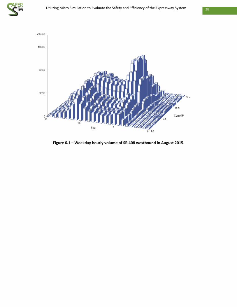
38 Utilizing Micro Simulation to Evaluate the Safety and Efficiency of the Expressway System
Figure 6.1 – Weekday hourly volume of SR 408 westbound in August 2015.

39 Utilizing Micro Simulation to Evaluate the Safety and Efficiency of the Expressway System
Figure 6.2 – Weekday occupancy of SR 408 westbound.
6.1.2 Key segment
After selecting SR 408, the next step was deciding the key study segment. Based on the weekday
occupancy of SR 408 in August 2015 (see Figure 6.2 and Appendix C-1), the congestion
conditions of SR 408 can be summarized as follows:
1. The congestion on the westbound lanes was more severe than that on the eastbound
lanes, and the most congested period of the westbound segment was around 7:00 A.M.
to 9:00 A.M.
2. The most congested segment is between milepost 10 and 16. To select a key segment for
potential safety improvement, the congested MP 12.1 to MP 13.3 segment on the
westbound lanes was chosen. This segment contains a weaving segment that was
identified in Chapter 4 as having more crashes than other segment types. The length of
the weaving segment is only about 1,400 feet in which diverging and merging
maneuvers cannot be separately conducted.
3. The congestion intensity changed by time. When approaching peak hours, the congestion
intensity gradually increased. Once the peak time passed, the congestion became less
severe. Therefore, in addition to studying the congestion period, there was also a need
to study the time before and after the congestion period. Hence, one and half hours
before and after the peak hours were also analyzed. The study period was from 6:30
A.M. to 10:30 A.M.
The weekday traffic data from August 2015 was selected to represent the average traffic
condition of the whole year. The main traffic on SR 408 is commuting traffic, so the weekday

40 Utilizing Micro Simulation to Evaluate the Safety and Efficiency of the Expressway System
traffic condition on SR 408 does not vary considerably across months. Figure 6.3 displays the
6:30 A.M. to 10:30 A.M. weekday average hourly volumes of a section whose milepost is 12.6 on
westbound of SR 408. The average hourly volume over 12 months in 2015 was 6,521 vehicles,
and the standard deviation was 273 vehicles. The weekday hourly volume in August was 6,586
vehicles, which was almost the same as the average hourly volume over a year.
Figure 6.3 – Weekday hourly volume in 2015.
6.2 Network Coding
The two basic components of the VISSIM roadway network are links and connectors. The links
represent roadway segments and are connected to other links by connectors. Vehicles cannot
travel from one link to another without connectors attached. For each link, several properties
must be specified: (1) number of lanes for the segment; (2) behavior type—there are six types of
behavior in total, and freeway (free lane selection) was selected in this project; (3) lane width,
set as 12.0 feet; and (4) gradient, set as 0% since the study segment is flat. Curvatures of the
studied segment were coded through adjusting the shape of links and connectors to follow the
roadway shapes in the background Bing maps, which is toggled in VISSIM. Finally, the coded
expressway segment could accurately represent the geometric characteristics of the studied
expressway segment. Figure 6.4 displays the coded segment with the background map. Links are
blue and connectors are red.
0
1000
2000
3000
4000
5000
6000
7000
8000
1 2 3 4 5 6 7 8 9 10 11 12
Hourly V
olu
me
Month
Hourly Volume

41 Utilizing Micro Simulation to Evaluate the Safety and Efficiency of the Expressway System
Figure 6.4 – Coded freeway section with background image.
In order to obtain traffic information from the VISSIM network, data collection points were
added in the simulation network. They were installed at the exact location of field MVDS
detectors to capture simulated traffic data. A data collection point recorded the time when the
front of a car reaches the point, the time when the rear of a car leaves the point, vehicle type,
speed, acceleration, etc. One data collection point can only catch traffic information for one
lane. Hence, if a segment has several lanes, multiple data collection points should be placed on
that segment. Figure 6.5 shows partial coded data collection points. The first letter of the name
stands for lane type: Mainline (m), Ramp (r), Toll Plaza Express (e), and Toll Plaza Cash (c). The
number following the lane type is milepost. The numbers in parentheses are lane id. The
innermost lane’s id is 1. By coding data collection points in this way, the simulation output data
can be easily processed.
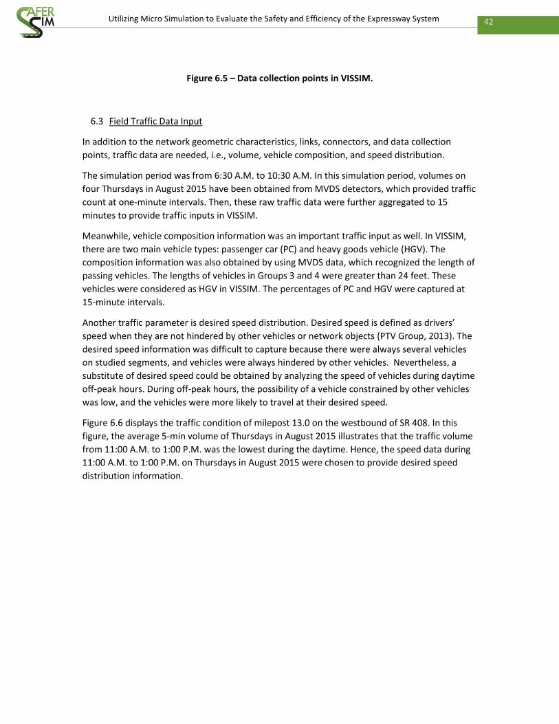
42 Utilizing Micro Simulation to Evaluate the Safety and Efficiency of the Expressway System
Figure 6.5 – Data collection points in VISSIM.
6.3 Field Traffic Data Input
In addition to the network geometric characteristics, links, connectors, and data collection
points, traffic data are needed, i.e., volume, vehicle composition, and speed distribution.
The simulation period was from 6:30 A.M. to 10:30 A.M. In this simulation period, volumes on
four Thursdays in August 2015 have been obtained from MVDS detectors, which provided traffic
count at one-minute intervals. Then, these raw traffic data were further aggregated to 15
minutes to provide traffic inputs in VISSIM.
Meanwhile, vehicle composition information was an important traffic input as well. In VISSIM,
there are two main vehicle types: passenger car (PC) and heavy goods vehicle (HGV). The
composition information was also obtained by using MVDS data, which recognized the length of
passing vehicles. The lengths of vehicles in Groups 3 and 4 were greater than 24 feet. These
vehicles were considered as HGV in VISSIM. The percentages of PC and HGV were captured at
15-minute intervals.
Another traffic parameter is desired speed distribution. Desired speed is defined as drivers’
speed when they are not hindered by other vehicles or network objects (PTV Group, 2013). The
desired speed information was difficult to capture because there were always several vehicles
on studied segments, and vehicles were always hindered by other vehicles. Nevertheless, a
substitute of desired speed could be obtained by analyzing the speed of vehicles during daytime
off-peak hours. During off-peak hours, the possibility of a vehicle constrained by other vehicles
was low, and the vehicles were more likely to travel at their desired speed.
Figure 6.6 displays the traffic condition of milepost 13.0 on the westbound of SR 408. In this
figure, the average 5-min volume of Thursdays in August 2015 illustrates that the traffic volume
from 11:00 A.M. to 1:00 P.M. was the lowest during the daytime. Hence, the speed data during
11:00 A.M. to 1:00 P.M. on Thursdays in August 2015 were chosen to provide desired speed
distribution information.

43 Utilizing Micro Simulation to Evaluate the Safety and Efficiency of the Expressway System
Figure 6.6 – Average 5-min volume on Thursdays in August 2015.
After deciding the time period for collecting desired speed distribution data, field cumulative
speed distributions were formulated with the MVDS speed data by different lane types:
mainline, on-ramp, off-ramp, toll plaza express lane, and toll plaza cash lane. Figure 6-7 displays
an example of the speed distribution for the mainline.
Figure 6.7 – Cumulative speed distribution for mainline.

44 Utilizing Micro Simulation to Evaluate the Safety and Efficiency of the Expressway System
The MVDS data provided the average speed for all vehicle types, but did not provide speed for
different vehicle types (i.e., PC and HGV). Nevertheless, VISSIM had to specify desired speed
distributions for different vehicle types. Therefore, one assumption was made to facilitate the
calculation of desired speed distributions: the average speed of PC was 8.1 mph higher than that
of HGV (Johnson & Murray, 2010).
From the MVDS data, it can be found that the average HGV percentage of the study segment
was about 10%. Supposing x is the speed of PC, the speed for HGV is equal to (x-8.1), and the
average speed provided by MVDS is y. Then,
0.9 x+0.1 (x-8.1) =y (6.1)
From Equation (6.1), the passenger car speed was found to be about y+0.8, and the HGV speed
was around y-7.3. Then the desired speed distribution of PC and HGV were acquired separately.
Figure 6.8 gives an example of the mainline desired speed distribution for PC and HGV.
(a) Desired speed distribution of PC
45 Utilizing Micro Simulation to Evaluate the Safety and Efficiency of the Expressway System
(b) Desired speed distribution of HGV
Figure 6.8 – Mainline desired speed distribution of (a) PC and (b) HGV.
6.4 VISSIM Network Calibration and Validation
After the required VISSIM elements were set up, network calibration and validation were
conducted. If there was a big difference between field traffic and VISSIM simulated traffic, the
traffic condition in the simulation network would fail to represent the real network, and the
tests based on simulation would not be not valid. Hence, calibrating and validating VISSIM traffic
are among the most important and basic tasks in the process of building a simulation network.
Only after a simulation network is satisfactorily calibrated and validated can the network be
used for further application, such as safety improvement and efficiency test.
Geoffrey E. Havers (GEH) was calculated to calibrate the VISSIM simulation network by
comparing simulated volume and field volume (Dowling et al., 2004). The definition of GEH is as
follows:
2( )
( ) / 2
E VGEH
E V
(6.2)
where E is simulated volume (vehicles per hour) and V is field volume (vehicles per hour). If
more than 85% of the measurement locations’ GEH values are less than 5, then the simulated
volume would accurately reflect the field volume (Yu & Abdel-Aty, 2014).
For the network validation, the absolute speed difference between the simulated traffic and
field traffic was taken as validation index. According to Nezamuddin et al. (2011), the absolute
value of speed difference should be within 5.0 mph for 85% of the checkpoints.

46 Utilizing Micro Simulation to Evaluate the Safety and Efficiency of the Expressway System
Previous studies have found that the desired lane change distance (DLCD) for weaving segments
in VISSIM was different from other segments and was also different from the default value of
VISSIM (200 meters) (Koppula, 2002; Woody, 2006). Hence, the DLCD was adjusted to get a
better validation result. It was set from 200 to 1000 meters, with an increment of 100 meters.
The result showed that the VISSIM network was better calibrated and validated when DCLD was
700 meters.
After excluding 30 minutes of VISSIM warm-up time and 30 minutes of cool-down time, a
total of 180 minutes of VISSIM data were put into use. Table 6.1 shows an example of GEH
values for the ramp and mainline of MP 13.0, which is located at the beginning of a weaving
segment. The table shows that the section was well calibrated. Only three out of 24
observations’ GEHs were higher than 5.0, among which two observations’ GEHs were just 0.34
higher than 5.0.
In this simulation run, 94.4% observations’ GEH were less than 5.0. The difference between
the sum of all link simulation flows and that of all link field flows is 3,616, which was only 1.50%
of the sum of all link field flows. Meanwhile, the average GEH for the sum of all link counts was
2.05. Furthermore, a total of 10 simulation runs with different random seeds has been
conducted to confirm the calibration result. Ten simulation runs’ results showed that the
average GEH was 1.97 and 96.4% observations’ GEHs were less than 5. Hence, the VISSIM
calibration target was reached.
Table 6.1 – Sample of GEH values for calibration.
Time Interval
MP 13.0 Ramp MP 13.0 Mainline
F_ Vol* V_ Vol# Abs(Dif) GEH F_ Vol V_ Vol Abs(Dif) GEH
3 518 528 10 0.44 6461 6380 81 1.01 4 658 528 130 5.34 7862 7848 14 0.16 5 642 608 34 1.36 8043 8012 31 0.35 4 554 472 82 3.62 7526 6784 742 8.77 5 504 552 48 2.09 7069 7056 13 0.15 6 540 440 100 4.52 7405 7156 249 2.92 7 514 428 86 3.96 6894 7028 134 1.61 8 448 464 16 0.75 6417 6284 133 1.67 9 434 420 14 0.68 5021 5160 139 1.95 10 397 372 25 1.27 4711 4632 79 1.16 11 450 492 42 1.94 4472 4484 12 0.18 12 395 352 43 2.22 4511 4600 89 1.32 13 518 528 10 0.44 6461 6380 81 1.01 14 658 528 130 5.34 7862 7848 14 0.16 Average 642 608 34 1.36 8043 8012 31 0.35
* Field volume
# VISSIM simulation volume

47 Utilizing Micro Simulation to Evaluate the Safety and Efficiency of the Expressway System
Once it was confirmed that the VISSIM network was well calibrated, the validation was done
based on speed comparisons between VISSIM and field traffic data at 15-minute intervals. Table
6.2 displays an example for error of speeds at three locations, including two mainline sections
and one toll plaza cash section. Results shown in the table prove that simulated speeds were
satisfactorily validated and that the errors are within acceptable ranges.

48 Utilizing Micro Simulation to Evaluate the Safety and Efficiency of the Expressway System
Table 6.2 – Speed differences for validation.
Time
Interval MP Type F_speed* V_speed# Abs(speed_dif)*
3 12.6 Mainline 61.91 55.71 6.20
4 12.6 Mainline 56.85 47.78 9.07
5 12.6 Mainline 40.56 41.38 0.82
6 12.6 Mainline 37.46 40.94 3.48
7 12.6 Mainline 48.41 45.76 2.65
8 12.6 Mainline 54.65 53.72 0.94
9 12.6 Mainline 51.24 51.53 0.29
10 12.6 Mainline 54.4 56.22 1.82
11 12.6 Mainline 62.31 59.81 2.50
12 12.6 Mainline 62.25 59.78 2.48
13 12.6 Mainline 58.05 60.63 2.58
14 12.6 Mainline 57.34 60.42 3.08
3 13.0 Mainline 62.51 59.95 2.57
4 13.0 Mainline 59.07 58.57 0.50
5 13.0 Mainline 53.03 52.25 0.78
6 13.0 Mainline 49.65 51.3 1.65
7 13.0 Mainline 54.93 59.5 4.57
8 13.0 Mainline 61.02 60.28 0.74
9 13.0 Mainline 55.42 60.64 5.22
10 13.0 Mainline 60.89 60.84 0.05
11 13.0 Mainline 63.76 60.66 3.10
12 13.0 Mainline 63.16 61.4 1.77
13 13.0 Mainline 62.03 61.3 0.73
14 13.0 Mainline 62.42 61.05 1.37
* Absolute value of speed difference
Additionally, nine more runs were carried out to confirm the validation result. Overall, 86.46%
observations’ absolute values of speed difference were less than 5.0 mph. Therefore, the VISSIM
network was successfully validated.

49 Utilizing Micro Simulation to Evaluate the Safety and Efficiency of the Expressway System
6.5 Summary
This project aims to improve the safety of a key segment. Both congestion and complicated
geometric design may increase crash risk. Hence, this chapter first identified the key segment
(milepost from 12.1 to 13.3 on westbound SR 408), in which a weaving segment exists. Weaving
segments have been proven to have higher crash potential than other segment types (see
Chapter 4).
Subsequently, a VISSIM network was built based on the geometric characteristics of a study
segment and the corresponding MVDS traffic data on Thursdays in August 2015. In order to
verify that the traffic condition of the simulation network was consistent with that of the field
network, the simulation network was calibrated and validated. The results showed that both the
calibration and validation requirements were satisfactorily met.

50 Utilizing Micro Simulation to Evaluate the Safety and Efficiency of the Expressway System
7 Traffic Safety Improvement for a Congested Weaving Segment
7.1 Introduction
Once the crash mechanisms of weaving segments have been found, countermeasures can be
proposed based on crash mechanisms. One possible method to improve the safety of weaving
segments is ATM, which is able to dynamically manage roadway facilities based on the prevailing
and predicted traffic conditions. Plenty of practitioners and researchers have proven that ATM
has the capability to provide safer and smoother traffic (Abdel-Aty et al., 2006; Bhouri &
Kauppila, 2011). Among ATM strategies, RM and VSL are widely used approaches. The basic
concept of the RM algorithm is adjusting on-ramp entering volume based on the mainline’s
traffic operational conditions. As for the VSL, the speed limit usually changes according to traffic
or weather conditions.
7.2 ATM Strategy Algorithm
7.2.1 Ramp Metering Algorithm
The concept behind the traditional ALINEA is to determine an on-ramp metering rate by the
road occupancy observed at the downstream of a merge area and a pre-specified critical
occupancy (Papageorgiou et al., 1991). This study adopts a modified ALINEA that additionally
considers safety conditions. The RM rate is based on occupancy and the crash risk of the studied
weaving segment. Previous studies stated that the occupancy detector should be placed at a
location where the congestion caused by on-ramp traffic can be detected, and put the
occupancy detector between 130 feet and 1,640 feet downstream of on-ramp noses (Chu &
Yang, 2003). This study put the occupancy detector 330 feet downstream of the on-ramp nose.
The metering rate at time step k is calculated in Equation (7.1):
1 1ˆ( ) ( 1) ( ) ( )R k s kr k r k K o o K p p (7.1)
where 𝑟(𝑘) is the metering rate (veh/h) at time interval k, 𝑟(𝑘 − 1) the metering rate at the
previous time interval k-1, 𝐾𝑅 the occupancy regulator parameter (veh/h), �� the critical
occupancy (%), 𝑜𝑘−1 the occupancy (%) at time interval k-1, 𝐾𝑆 the safety regulator parameter
(veh/h), 𝑝𝑘−1 the crash risk at the time interval k-1, and �� the critical crash risk.
The RM is achieved by adjusting the timing of the ramp signal, which is set at the end of the on-
ramp. The metering signal permits on-ramp vehicles to enter the weaving segment only when
the signal turns green. Otherwise, vehicles are required to stop at the signal and wait for a green
phase. The green-phase duration at time interval k, 𝑔(𝑘), is calculated as follows:
( )
( ) .sat
r kg k C
r
(7.2)
min max( )g g k g (7.3)

51 Utilizing Micro Simulation to Evaluate the Safety and Efficiency of the Expressway System
where C is the fixed cycle time (10 seconds), 𝑟𝑠𝑎𝑡 the ramp saturation flow (1800 veh/(h.lane))
(Bhouri et al., 2013), 𝑔𝑚𝑖𝑛 is 3 seconds, and 𝑔𝑚𝑎𝑥 the maximum green-phase duration (10
seconds). Meanwhile, in order to prevent the RM rate from increasing greatly and resulting in a
large amount of vehicles entering the mainline at time interval k, the maximum increment of
𝑟(𝑘) for each time interval is set to be 60 veh/h.
7.2.2 Variable Speed Limit Strategy
The crash analysis model for weaving segments in Chapter 5 found that the speed difference
between the upstream and downstream of a segment is positively related to the crash risk of
this segment. Meanwhile, several studies have found that VSL is capable of reducing speed
variation (Rämä, 1999; Kwon et al., 2007). Hence, the implementation of VSL might reduce crash
risk. In this study, when crash risk is higher than the critical crash risk (��), VSL at the upstream
and the downstream of the congested weaving segment are activated to reduce the speed
difference between the beginning and the end of the weaving segment.
7.3 Experiment Design
There were four parameters in the modified ALINEA algorithm that needed to be calibrated: the
critical occupancy (o), the occupancy regulator parameter (𝐾𝑅), the critical crash risk (��), and
the safety regulator parameter (𝐾𝑆). These parameters were set as follows:
1. In previous studies, the critical occupancy (��) was set between 17% and 23%, and it has
been found that a higher value of the critical occupancy ensures better safety benefits
(Abdel-Aty et al., 2007). For this study, the critical occupancy was set to be 23%.
2. The range of the occupancy regulator parameter (𝐾𝑅) used in previous studies varied from
70 to 120 veh/h. But it did not have significant effects on the metering rate (Papamichail
et al., 2010). This study used 70 veh/h.
3. In order to reduce the false alarm percentage, the threshold (��) of identifying a crash is set
to be 0.15. When the threshold is 0.15, the specificity of the crash estimation model in
the previous chapter was 0.973, and the false positive rate was 0.027. That meant only
2.7% of non-crash events were falsely identified as crash events.
4. The safety regulator parameter (𝐾𝑆) was set to be 0 and then to be 2.5 × 10³. Setting the
value of 𝐾𝑆 is very important. If the value 𝐾𝑆 is too small, the crash risk would not have a
significant impact on RM rate; if the value is too large, the RM rate might substantially
change because of a small variation in crash risk. When 𝐾𝑆 was set to be 0, the ALINEA
algorithm was the same as the traditional ALINEA algorithm. This study supposes that
when the conditional crash risk reaches the highest value, the RM rate is decreased by
180 veh/h, that is one second of green phase time. The maximum conditional crash risk
for the weaving segment without ATM control is around 0.22. Then,

52 Utilizing Micro Simulation to Evaluate the Safety and Efficiency of the Expressway System
maxˆ 180sK p p (7.4)
3
max
180 1802.5 10
ˆ 0.15 0.22sK
p p
(7.5)
RM might result in long travel times for on-ramp vehicles (Kotsialos & Papageorgiou, 2004).
Hence, there was a need to increase the green phase time when there were plenty of vehicles
piling up on ramps. The updated green phase time (𝑔′) was set as
10
1 10 20
2 20 30
3 30
g Queue
g Queueg
g Queue
g Queue
(7.6)
where g is calculated based on Equation (7.2), and Queue is the number of vehicles in the queue
of the on-ramp. On the other hand, merely increasing the green phase time might not be
enough, as entering vehicles needed sufficient gaps in order to merge into the mainline. Hence,
it may be better to simultaneously set the upstream variable speed limit in order to provide a
bigger gap for entering vehicles.
The parameters used to determine the ramp metering rate were collected from the data
collection points in the VISSIM simulation network. Then the COM interface implemented Visual
Basic for Applications (VBA) from Excel to adjust the green and red signal timing of RM.
The field speed limit of the studied weaving segment is 55 mph. The speed limit at the upstream
was set to be 45, 50, or 55 mph. The speed limit at the downstream was set to be 55, 60, or 65
mph. The application of VSL in microsimulation is carried out by changing the desired speed
distributions. The field desired speed data can be obtained from the MVDS detectors on the
studied weaving segment. As for other desired speed distributions of VSLs, it is supposed that if
the speed limit changes (by decreasing or increasing) by n mph, all vehicles’ speeds will
accordingly change by n mph. Hence, based on this assumption and the field desired speed
distribution, the desired speed distributions of different speed limits can be obtained.
The locations of RM and VSLs are shown in Figure 7.1. The detectors were used to measure the
occupancy (o), and data collection points collected other traffic information, i.e., traffic count
and speed.

53 Utilizing Micro Simulation to Evaluate the Safety and Efficiency of the Expressway System
Figure 7.1 – Studied weaving segment microsimulation network.
There were 13 cases in total; the detailed information is listed in Table 7.1. Case 1 is the non-
control case, Cases 2-4 are RM strategies, Cases 5-12 are VSL strategies, and Case 3 is the
integrated RM-VSL strategy.
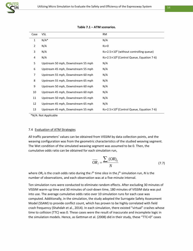
54 Utilizing Micro Simulation to Evaluate the Safety and Efficiency of the Expressway System
Table 7.1 – ATM scenarios.
Case VSL RM
1 N/A* N/A
2 N/A Ks=0
3 N/A Ks=2.5×10⁶ (without controlling queue)
4 N/A Ks=2.5×10⁶ (Control Queue, Equation 7-6)
5 Upstream 50 mph, Downstream 55 mph N/A
6 Upstream 45 mph, Downstream 55 mph N/A
7 Upstream 55 mph, Downstream 60 mph N/A
8 Upstream 55 mph, Downstream 65 mph N/A
9 Upstream 50 mph, Downstream 60 mph N/A
10 Upstream 45 mph, Downstream 60 mph N/A
11 Upstream 50 mph, Downstream 65 mph N/A
12 Upstream 45 mph, Downstream 65 mph N/A
13 Upstream 45 mph, Downstream 55 mph Ks=2.5×10⁶ (Control Queue, Equation 7-6)
*N/A: Not Applicable
7.4 Evaluation of ATM Strategies
All traffic parameters’ values can be obtained from VISSIM by data collection points, and the
weaving configuration was from the geometric characteristics of the studied weaving segment.
The Wet condition of the simulated weaving segment was assumed to be 0. Then, the
cumulative odds ratio can be obtained for each simulation run,
( )ijij
OROR
N
(7.7)
where ORij is the crash odds ratio during the ith time slice in the jth simulation run, N is the
number of observations, and each observation was at a five-minute interval.
Ten simulation runs were conducted to eliminate random effects. After excluding 30 minutes of
VISSIM warm-up time and 30 minutes of cool-down time, 180 minutes of VISSIM data was put
into use. The average cumulative odds ratio over 10 simulation runs for each case was
computed. Additionally, in the simulation, the study adopted the Surrogate Safety Assessment
Model (SSAM) to provide conflict count, which has proven to be highly correlated with field
crash frequency (Shahdah et al., 2014). In each simulation, there existed “virtual” crashes whose
time to collision (TTC) was 0. These cases were the result of inaccurate and incomplete logic in
the simulation models. Hence, as Gettman et al. (2008) did in their study, these “TTC=0” cases

55 Utilizing Micro Simulation to Evaluate the Safety and Efficiency of the Expressway System
were excluded from further analysis. Meanwhile, average travel time was obtained to check the
network’s efficiency. The average results over 10 simulation runs are shown in Table 7.2.
Overall, compared to the non-control case (Case 1), the safety of the congested weaving
segment was improved by the ATM strategies. For 9 out of 12 cases, their conflict numbers were
reduced and the average odds ratios were less than 1. In addition to improving the safety at the
weaving segment, the safety of the non-weaving segments, which were located upstream and
downstream of the weaving segment, was also improved significantly (more than 10%) in 7 out
of 12 cases. Except for three cases (i.e., 2, 7, and 8), the average travel time of most cases
increased because on-ramp vehicles were delayed or the average speed was reduced or both.

56 Utilizing Micro Simulation to Evaluate the Safety and Efficiency of the Expressway System
Table 7.2 – ATM simulation results
Case
Weaving Non-weaving Whole
Conflict Conflict
reduced % OR Conflict
Conflict
reduced % ATT#
ATT reduced
%
1 705 N/A* 1.00 59 N/A 98.3 N/A
2 653 -7.3 1.01 38 -35.6 97.9 -0.4
3 555 -21.2 0.95 41 -30.5 113.7 15.7
4 621 -11.9 0.92 40 -31.7 101.4 3.2
5 639 -9.3 0.88 62 5.8 100.1 1.9
6 575 -18.4 0.82 43 -26.9 101.3 3.1
7 705 0.1 1.00 59 -0.3 97.7 -0.5
8 705 0.0 1.00 60 1.4 97.4 -0.8
9 639 -9.3 0.88 63 7.7 99.8 1.5
10 575 -18.4 0.82 44 -25.2 101.1 2.9
11 639 -9.3 0.88 63 7.8 99.6 1.4
12 575 -18.4 0.82 43 -26.1 101.0 2.8
13 586 -16.8 0.94 43 -27.6 105.0 6.9
* N/A: Not Applicable
# Average Travel Time in seconds
In the traditional ALINEA case (Case 2), the average conflict count was decreased by 7.3%, but
the average odds ratio was 1.01, which means the crash odds increased by 1%. On the other
hand, the modified ALINEA without controlling queue length (Case 3) decreased conflict by
21.2% and decreased odds by 5%. And for the modified ALINEA whose queue length was
controlled (Case 4), it decreased conflict by 11.9% and decreased odds 8%. Since the modified
ALINEA cases (i.e., 3 and 4) adjusted the RM rate based on traffic operation and safety
conditions simultaneously, they were able to better improve safety than the traditional ALINEA
(Case 2). Though the safety benefit of the modified ALINEA without controlling queue length
(Case 3) performed well among ALINEAs, the good performance was at the cost of travel time. It
increased the average travel time by 15.7%.
Examination of the results in Table 7.2 clearly shows that setting VSL at the downstream of the
weaving segment did not improve the safety of the weaving segment. The main reason was that
the high speed limit at the downstream of weaving segment does not necessarily increase the
speed at the end of the weaving segment, which is mainly impacted by traffic conditions in the

57 Utilizing Micro Simulation to Evaluate the Safety and Efficiency of the Expressway System
weaving segment. Hence, even though the speed limit at the downstream of the weaving
segment was increased, the speed at the end of the weaving segment was still low, the
difference between the beginning and the end of the weaving segment remained the same, and
the crash risk was almost constant. On the contrary, setting the VSL at the upstream of the
weaving segment reduced both conflict number and crash odds. Furthermore, compared to
setting the upstream weaving segment VSL to 50 mph, the 45 mph VSL improved the safety
more. It is not hard to understand: the lower the speed limit of the upstream segment, the
lower the speed at the beginning of the weaving segment, and the lower the speed difference.
And the lower speed difference produced lower crash risk.
Though the 45 mph VSL strategy was capable of improving safety without significantly increasing
the average travel time, the effectiveness of VSL can be impacted by the compliance level. The
VSL system might fail to enhance traffic safety under low compliance conditions (Yu & Abdel-
Aty, 2014). In contrast, the modified ALINEA without controlling queue length (Case 3) improved
safety at the expense of increased average travel time, but there is no compliance issue for RM.
Meanwhile, only controlling the queue length of the modified ALINEA worsened the impact of
the modified ALINEA on the weaving segment’s safety. Therefore, the RM-VSL was needed to
enhance and combine the advantages of VSL and RM. The simulation results demonstrated that
the RM-VSL (Case 13) significantly decreased the average travel time by 8.7 seconds when
compared to the modified ALINEA without controlling queue length (Case 3). Meanwhile, the
RM-VSL (Case 13) was as good as the modified RM without controlling queue length (Case 3) in
enhancing the safety of the weaving segment.
Additionally, to test the level of agreement between the conflict count and average odds ratio
value, the Spearman’s rank correlation test, a non-parametric correlation, was used since there
were only 13 cases in total. A higher Spearman’s rank correlation coefficient indicates that there
is a high dependence between two variables. A coefficient of 1.0 represents a perfect
agreement, and that of 0 indicates no correlation (Gettman et al., 2008). The result suggested
that the relationship between conflict count and average odds ratio value (Spearman’s rank
coefficient=0.670, p=0.01) was statistically significant. This confirms that the safety of the
simulation is consistent with the crash risk, whose model was built based on field data. But
there were still small inconsistencies between conflicts and OR . The 45 mph VSL (Case 6) was
better than the modified ALINEA without controlling queue (Case 3) since Case 6’s crash odds
compared to the crash odds under base condition were lower than the odds ratio of Case 3. On
the other hand, the conflict count of the modified ALINEA without controlling queue (Case 3)
was slightly less than that of the 45 mph VSL. Meanwhile, in the modified ALINEA without
controlling queue case (Case 3), the percentage of conflict count reduced was higher than the
percentage of odds reduced.
Table 7.2 gives cumulative results and does not show detailed information for each step. In
order to better understand the effects of ATM strategies on crash risk for each time slice, Figure
7.2 shows the average crash odds ratio of 10 runs for the non-control case (Case 1), the
traditional ALINEA (Case 2), the modified ALINEA without controlling queue length (Case 3), 45
mph upstream VSL (Case 6), and RM-VSL (Case 13).

58 Utilizing Micro Simulation to Evaluate the Safety and Efficiency of the Expressway System
Figure 7.2 – Crash risk for different cases
In Figure 7.2, the crash risk curve of the traditional ALINEA (Case 2) almost overlaps with that of
the non-control case (Case 1). This indicates that the traditional ALINEA (Case 2) did not have a
significant impact on the safety of the studied weaving segment in each step. The result is not
coherent with the previous studies by Lee et al. (2006) and Abdel-Aty and Gayah (2008), which
have found that the traditional ALINEA significantly improved real-time safety. This might be
because of the difference in study subjects. Their studies focused on freeway segments without
distinguishing the segment type, but this study only concentrated on weaving segments. On
weaving segments, the traffic behavior and crash mechanisms are not the same as other non-
weaving segments.
The crash risk curve of 45 mph VSL (Case 6) is always lower than that of modified RM without
controlling queue length (Case 3). It means that the 45 mph VSL outperformed the RM by
providing lower crash risks. The reasons might be as follows:
1. When a crash risk is higher than the critical crash risk, the VSL strategy reacts more
quickly and effectively than the RM. The speed limit was able to change immediately
using VSL; however, the RM adjusted the ramp metering rate gradually.
2. Though RM had the capability to reduce speed variances, the VSL can decrease the
variance of speed more. In the simulation run with the random seed of 17, the average
speed difference of the non-control case (Case 1) was 6.8 mph, and the average speed
differences of the 45 mph VSL (Case 6) and the RM without controlling queue length
(Case 3) were 4.6 and 5.7 mph, respectively. Other simulation runs with different
random seeds also had similar results.
0.40
0.50
0.60
0.70
0.80
0.90
1.00
1.10
30 50 70 90 110 130 150 170 190
Crash Odds Ratio
Case 1 Case 2 Case 3 Case 6 Case 13
59 Utilizing Micro Simulation to Evaluate the Safety and Efficiency of the Expressway System
Another finding from Figure 7.2 is this: when the crash risk was lower than the critical crash risk
and the speed limit was returned to 55 mph, the 45 mph VSL at the upstream segment (Case 6)
consistently improved the safety of the studied weaving segment. Vehicles did not accelerate
significantly and rapidly when the speed limit changed from 45 mph to 55 mph. The vehicles
were impacted by vehicles ahead, which were still at low speeds. Meanwhile, when the crash
risk was reduced below the critical crash risk, the modified ALINEA without controlling queue
length (Case 3) also improved the real-time safety because the metering rate increased
gradually and the RM signal broke up platoons of entering vehicles. The same finding also
applies to RM-VSL case (Case 13).
7.5 Summary
Traffic conditions in weaving segments are complicated since traffic merges, diverges, and
weaves in limited spaces. The complication might result in a low capacity and a high crash risk in
weaving segments. In order to improve the safety of a congested weaving segment, ATM
strategies were applied in microsimulation. The simulation results show that several ATM
strategies were able to improve the safety of the studied weaving segment by providing lower
conflict numbers and lower crash odds.
From the perspective of safety, the modified ALINEA cases, which take both traffic operation
and safety into consideration, outperformed the traditional ALINEA algorithm. However, the
average travel time of the modified ALINEA without controlling queue was significantly higher
than the non-control case and also higher than the traditional ALINEA case. The modified
ALINEA, which controlled the queue length, shortened the average travel time, but impaired the
safety impact of the modified ALINEA algorithm.
Both the location and speed limit value of VSL are important. The VSL set downstream of the
studied weaving segment did not mitigate crash risks, but the upstream VSL significantly
enhanced the safety of the weaving segment. Meanwhile, the 45 mph VSL improved safety
better than the 50 mph VSL without a significant increase in average travel times. Though VSL
more effectively improved the safety compared to RMs, the VSLs have the potential problem of
compliance, whereas compliance is not a big concern with the RM strategy.
In order to reduce the average travel time of RM and mitigate the compliance issue of VSL, an
RM-VSL was proposed. In RM strategy, when the queue of an on-ramp was long, the ramp signal
green phase time was increased in order to reduce the queue, and the speed limit upstream of
the weaving segment was reduced to 45 mph in order to provide enough time gaps for entering
vehicles. The results indicate that the RM-VSL produced lower conflict numbers than the RM
with queue control and traditional RM, and that it substantially reduced the average travel time
when compared to RM without queue control.
60 Utilizing Micro Simulation to Evaluate the Safety and Efficiency of the Expressway System
8 Conclusion
The safety of expressways is of significant importance. In order to improve expressway safety,
crash-contributing factors were explored in this project. The majority of previous expressway
safety studies were based on ADT. If the traffic of an expressway has significant peak and non-
peak hours, its crash potential in one segment should be different from another segment, which
has the same ADT but the volume is the same for each hour. The studied expressways were
mainly used for commuting traffic, which has significant peak and non-peak patterns. Hence, in
addition to ADT, this project also applied AHT and microscopic traffic at five-minute intervals to
analyze crashes on expressway segments.
In all ADT-based, AHT-based, and microscopic-traffic-based safety studies, the results illustrated
that the existence of weaving segment could increase crash potential. It is not hard to
understand. Weaving segments are potential recurrent bottlenecks because the capacity of
weaving segments is much lower than that of basic expressway segments when controlling for
free-flow speed, number of lanes, etc. Meanwhile, they are one of the most complicated
segments, since on- and off-ramp traffic merges, diverges, and weaves in limited space. In
addition to finding the impact of segment type on safety, the ADT-based, AHT-based, and
microscopic-traffic-based safety studies were compared at three levels: total, hourly, and five-
minute intervals. The comparison results showed that the microscopic traffic (at five-minute
intervals) data was the most suitable traffic data if ATM was used to improve the safety of a
segment in real time.
Then, the crash mechanisms of weaving segments were analyzed using real-time safety analysis
based on microscopic traffic data at five-minute intervals. The model results showed that the
speed difference between the beginning and the end of a weaving segment had significantly
positive impacts on the crash risk of the following 5-10 minutes for weaving segments.
Meanwhile, the weaving influence length, which was mainly determined by the weaving volume
rate, was also positively related to crash potential. These findings indicate that if an ATM
strategy is able to reduce speed difference or weaving influence length or both, it could possibly
enhance the safety of weaving segments.
A congested weaving segment and its upstream and downstream segments on SR 408 were
filtered out to be the key segment of this study. Its average hourly volume in the studied time
period in 2015 was 6,521 vehicles, and the average occupancy during peak hours was about
25.0%. The heavy traffic might bring about high crash potential. Hence, this project built a well-
calibrated and validated VISSIM network to simulate the traffic condition of the studied weaving
segment during peak hours. Two types of ATM strategies, VSL and RM, were applied to the
studied weaving segment through COM interface. The simulation result showed that the
modified ALINEA cases, which take both traffic operation and safety into consideration,
outperformed the traditional ALINEA algorithm in improving safety. Meanwhile, the 45 mph
VSL, which was installed upstream of the weaving segment, improved safety better than other
VSL strategies.
Though VSL could improve the safety more effectively than RMs, the VSLs have the potential
problem of compliance, whereas the compliance is not a big concern in the RM strategy.
61 Utilizing Micro Simulation to Evaluate the Safety and Efficiency of the Expressway System
Therefore, in order to reduce the average travel time of RM and mitigate the compliance issue
of VSL, an RM-VSL was proposed. The results indicate that the RM-VSL produced lower conflict
numbers than the RM with queue control and traditional RM, and that it substantially reduced
the average travel time compared to RM without queue control.
This project also found that the relationship between the simulated conflict number and the
crash odds ratio was statistically significant. However, there were small inconsistencies between
the conflict count and the total crash risk. The variance might be due to the difference between
crash mechanisms and conflict mechanisms. This finding might inspire further research into the
relationship between crash and conflict mechanisms in the real-time perspective.
Overall, this project identified the weaving segments as expressway special facilities that have
different crash potential than other segments, found the crash mechanisms of weaving
segments, and then applied ATM to improve the safety of a congested weaving segment. In
addition to weaving segments, interchanges are also an important expressway facility; they
connect expressways with arterials. The traffic in interchanges has different traveling directions
and might conflict with each other. Hence, the crash potential in interchanges is high. In recent
years, several new types of interchange design have been proposed and built. For example, the
diverging diamond interchange (DDI) enables two directions of traffic on the arterials to cross to
the opposite side on both sides of the overpass. From the theoretical point of view, the DDI
design is able to decrease the number of conflict points and simplify the signal phase. However,
it may cause drivers confusion in the initial stages. Thus, the traffic safety of such new
interchange design must be thoroughly examined. Furthermore, simulation can also be
implemented to suggest better designs to improve the current interchange configuration.

62 Utilizing Micro Simulation to Evaluate the Safety and Efficiency of the Expressway System
APPENDIX A: MVDS System and Lane Configuration
Table A.1 – SR 408 westbound MVDS system and lane configuration.
Westbound Number of lanes Westbound Number of lanes
ID Milepost Mainline (w/ TP Express)
TP Cash
Ramp ID Milepost Mainline (w/ TP Express)
TP Cash
Ramp
1 1.2 2 29 11.6 4 1
2 1.4 2 30 12.1 5
3 1.6 3 2 31 12.6 5 2
4 2 3 1 32 13 5 1
5 2.4 3 1 33 13.3 3 2
6 2.7 2 1 34 13.6 3 4 1
7 3.2 2 2 35 14.2 5 1
8 3.6 2 1 36 14.4 4 1
9 4.3 3 2 37 14.5 5
10 4.6 4 38 15.2 5
11 4.9 3 1 39 15.7 5 1
12 5.3 3 1 40 15.9 4 1
13 5.9 3 2 1 41 16.1 4 2
14 6.3 3 2 42 16.5 5
15 6.8 3 43 17 3 2
16 7.3 3 1 44 17.8 3 1
17 7.4 4 45 18 3 1
18 7.6 3 1 46 18.4 2 1
19 8.1 3 1 47 18.8 2 1
20 8.4 3 1 48 19 2 1
21 8.9 3 1 49 19.4 2 2
22 9.2 3 1 50 19.7 3 1
23 9.7 3 1 51 19.9 2 1
24 9.9 2 2 52 20.7 3
25 10.3 3 1 53 20.8 2 1
26 10.6 4 54 21.8 2
27 10.9 4 2 55 22.3 2 1
28 11.3 5 1 56 22.7 2 1

63 Utilizing Micro Simulation to Evaluate the Safety and Efficiency of the Expressway System
Table A.2 – SR 417 northbound MVDS system and lane configuration.
Northbound Number of lanes Northbound Number of lanes
ID Milepost Mainline (w/ TP Express)
TP Cash
Ramp ID Milepost Mainline (w/ TP Express)
TP Cash
Ramp
1 5.9 2 29 23.9 2 1
2 6.2 2 2 30 24.5 2
3 7.2 2 2 31 25 2 1
4 7.5 2 1 32 26.1 2 3
5 8.2 2 33 26.9 4
6 9.4 2 1 34 27.3 3 2
7 10.1 2 1 35 27.9 3 1
8 10.6 2 1 36 28.1 3 2
9 11 2 2 37 28.5 3 1
10 12.2 2 38 28.7 4
11 13.1 3 2 39 29.5 3 1
12 13.9 2 1 40 30.2 2 1
13 14.5 2 41 31.2 2
14 15.2 4 42 31.9 2
15 15.6 2 1 43 32.5 2 1
16 16.4 2 44 33 1
17 16.6 2 1 45 33.3 4 1
18 17.9 2 1 46 33.6 4
19 18.2 2 47 34 3 2
20 18.8 2 1 48 34.6 3 1
21 19.3 2 1 49 35.2 3
22 20.4 2 50 35.5 2 2
23 20.9 2 51 36 3 2
24 21.3 2 1 52 36.4 4 2
25 22 2 1 53 36.7 3 1
26 22.5 2 1 54 36.9 3 1
27 23 2 1 55 37.2 3
28 23.6 2 1 56 37.7 2

64 Utilizing Micro Simulation to Evaluate the Safety and Efficiency of the Expressway System
Table A.3 – SR 417 southbound MVDS system and lane configuration.
Southbound Number of lanes Southbound Number of lanes
ID Milepost Mainline (w/ TP Express)
TP Cash
Ramp ID Milepost Mainline (w/ TP Express)
TP Cash
Ramp
1 5.9 2 29 24.2 2 1
2 6.2 2 2 30 24.5 2 1
3 7.2 2 1 31 24.9 2 1
4 7.5 2 2 32 26.1 3 2
5 8.2 2 33 26.9 4
6 9.4 2 1 34 27.3 3 1
7 10.3 2 2 35 27.9 4 1
8 10.7 2 1 36 28.1 3 1
9 11.2 3 1 37 28.5 3 2
10 12.2 2 38 28.7 4
11 13.2 2 1 39 29.5 3 1
12 13.9 2 1 40 30.2 2 1
13 14.7 2 41 31.2 2
14 15.2 3 42 31.9 2
15 15.6 2 2 43 32.5 2 1
16 16.4 2 44 32.9 1
17 16.6 2 1 45 33.1 3 2
18 17.7 2 1 46 33.6 3 2
19 18.2 2 47 34.5 3 1
20 18.8 2 1 48 34.8 3 1
21 19.5 2 1 49 35.2 3
22 20.4 2 50 35.5 2 1
23 20.9 2 51 36 2 2
24 21.3 2 1 52 36.4 3 1
25 22.2 2 1 53 36.7 2 1
26 23 3 54 37 2 1
27 23.2 2 1 55 37.2 2
28 23.5 2 1 56 37.7 2
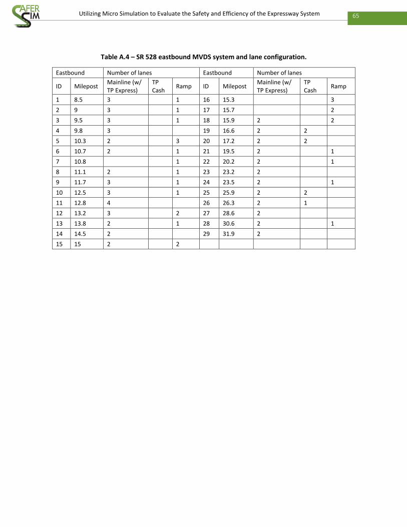
65 Utilizing Micro Simulation to Evaluate the Safety and Efficiency of the Expressway System
Table A.4 – SR 528 eastbound MVDS system and lane configuration.
Eastbound Number of lanes Eastbound Number of lanes
ID Milepost Mainline (w/ TP Express)
TP Cash
Ramp ID Milepost Mainline (w/ TP Express)
TP Cash
Ramp
1 8.5 3 1 16 15.3 3
2 9 3 1 17 15.7 2
3 9.5 3 1 18 15.9 2 2
4 9.8 3 19 16.6 2 2
5 10.3 2 3 20 17.2 2 2
6 10.7 2 1 21 19.5 2 1
7 10.8 1 22 20.2 2 1
8 11.1 2 1 23 23.2 2
9 11.7 3 1 24 23.5 2 1
10 12.5 3 1 25 25.9 2 2
11 12.8 4 26 26.3 2 1
12 13.2 3 2 27 28.6 2
13 13.8 2 1 28 30.6 2 1
14 14.5 2 29 31.9 2
15 15 2 2

66 Utilizing Micro Simulation to Evaluate the Safety and Efficiency of the Expressway System
Table A.5 – SR 528 westbound MVDS system and lane configuration.
Westbound Number of lanes Westbound Number of lanes
ID Milepost Mainline (w/
TP Express)
TP
Cash Ramp ID Milepost
Mainline (w/
TP Express)
TP
Cash Ramp
1 8.5 3 1 16 15.3 2 2
2 9.4 3 1 17 15.6 2 1
3 9.5 3 1 18 15.9 2 2
4 9.8 3 19 16.6 2 2
5 10.3 4 20 17.2 2 2
6 10.5 2 2 21 19.5 2 1
7 10.9 2 1 22 20.2 2 1
8 11 3 2 23 23.3 2
9 12 4 1 24 23.5 2 1
10 12.2 3 1 25 25.9 2 1
11 12.5 3 1 26 26.3 2 2
12 12.8 3 27 28.6 2
13 13.2 3 1 28 30.6 2 1
14 13.8 3 1 29 31.9 2
15 14.5 2

67 Utilizing Micro Simulation to Evaluate the Safety and Efficiency of the Expressway System
APPENDIX B Expressway Hourly Volume
Figure B.1 – Weekday hourly volume of SR 408 eastbound in August 2015.

68 Utilizing Micro Simulation to Evaluate the Safety and Efficiency of the Expressway System
Figure B.2 – Weekday hourly volume of SR 417 southbound in August 2015.
Figure B.3 – Weekday hourly volume of SR 417 northbound in August 2015.
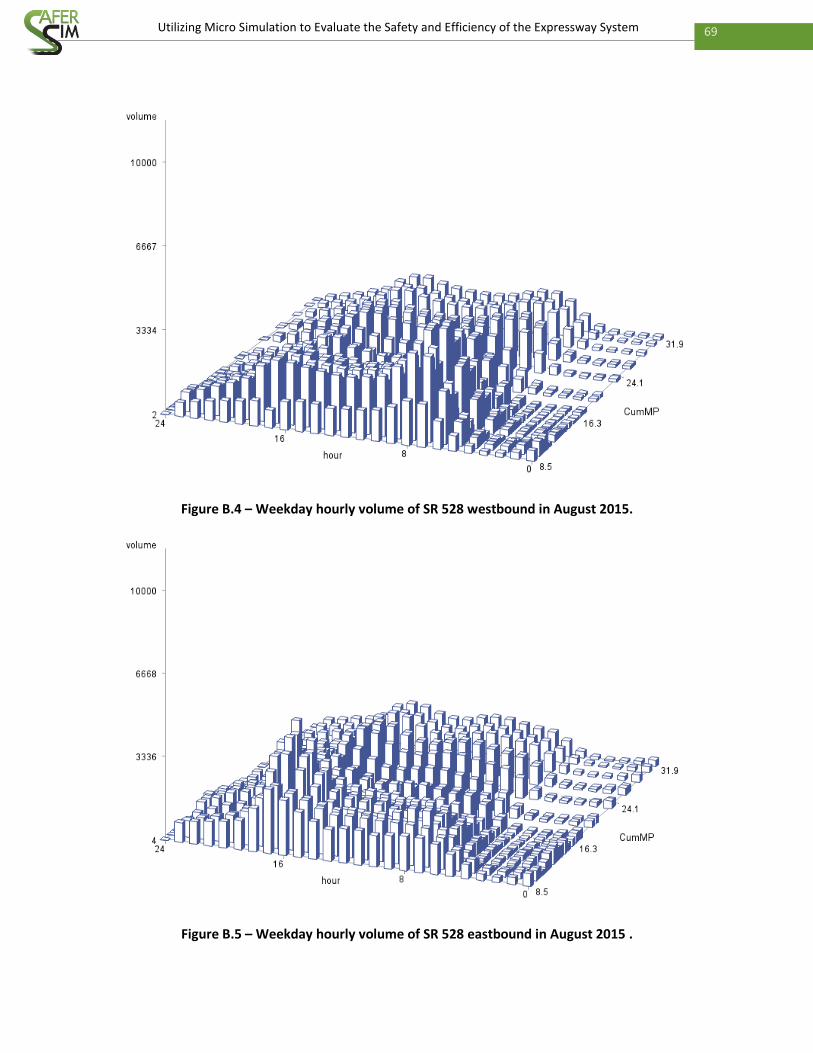
69 Utilizing Micro Simulation to Evaluate the Safety and Efficiency of the Expressway System
Figure B.4 – Weekday hourly volume of SR 528 westbound in August 2015.
Figure B.5 – Weekday hourly volume of SR 528 eastbound in August 2015 .
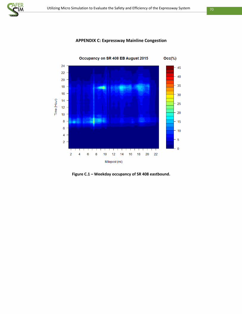
70 Utilizing Micro Simulation to Evaluate the Safety and Efficiency of the Expressway System
APPENDIX C: Expressway Mainline Congestion
Figure C.1 – Weekday occupancy of SR 408 eastbound.

71 Utilizing Micro Simulation to Evaluate the Safety and Efficiency of the Expressway System
Figure C.2 – Weekday occupancy of SR 417 southbound.

72 Utilizing Micro Simulation to Evaluate the Safety and Efficiency of the Expressway System
Figure C.3 – Weekday occupancy of SR 417 northbound.

73 Utilizing Micro Simulation to Evaluate the Safety and Efficiency of the Expressway System
Figure C.4 – Weekday occupancy of SR 528 westbound.
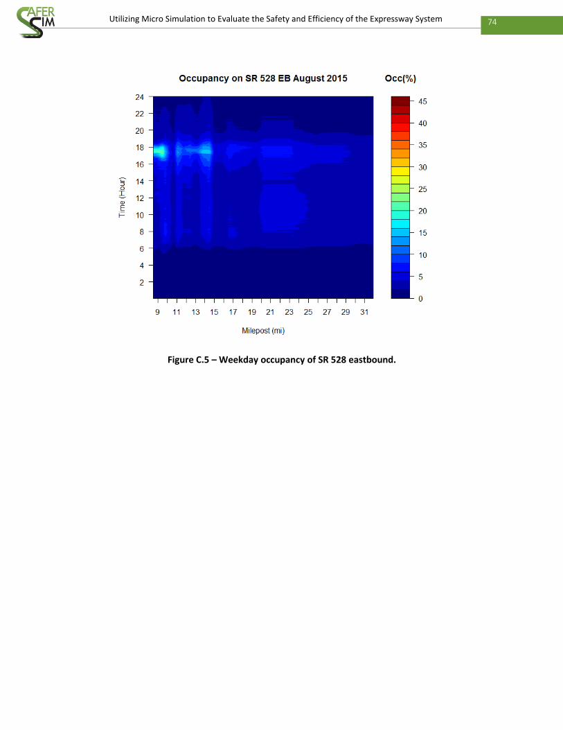
74 Utilizing Micro Simulation to Evaluate the Safety and Efficiency of the Expressway System
Figure C.5 – Weekday occupancy of SR 528 eastbound.

75 Utilizing Micro Simulation to Evaluate the Safety and Efficiency of the Expressway System
9 References
Abdel-Aty, M., Dhindsa, A., & Gayah, V. (2007). Considering various alinea ramp metering
strategies for crash risk mitigation on freeways under congested regime. Transportation
Research Part C: Emerging Technologies, 15 (2), 113-134.
Abdel-Aty, M., & Dhindsa, A. (2007). Coordinated use of variable speed limits and ramp
metering for improving safety on congested freeways. In: Proceedings of the Transportation
Research Board 86th Annual Meeting, Washington, DC.
Abdel-Aty, M., Dilmore, J., & Dhindsa, A. (2006). Evaluation of variable speed limits for real-time
freeway safety improvement. Accident Analysis & Prevention, 38 (2), 335-345.
Abdel-Aty, M., & Gayah, V. (2008). Comparison of two different ramp metering algorithms for
real-time crash risk reduction. In: Proceedings of the Transportation Research Board 87th
Annual Meeting, Washington, DC.
Abdel-Aty, M., Haleem, K., Cunningham, R., & Gayah, V. (2009). Application of variable speed
limits and ramp metering to improve safety and efficiency of freeways. In: Proceedings of
the 2nd International Symposium on Freeway and Tollway Operations, Honolulu, Hawaii.
Abdel-Aty, M., & Pemmanaboina, R. (2006). Calibrating a real-time traffic crash-prediction
model using archived weather and its traffic data. IEEE Transactions on Intelligent
Transportation Systems, 7 (2), 167-174.
Abdel-Aty, M., Uddin, N., & Pande, A. (2005). Split models for predicting multivehicle crashes
during high-speed and low-speed operating conditions on freeways. Transportation
Research Record: Journal of the Transportation Research Board (1908), 51-58.
Abdel-Aty, M., Uddin, N., Pande, A., Abdalla, F., & Hsia, L. (2004). Predicting freeway crashes
from loop detector data by matched case-control logistic regression. Transportation
Research Record: Journal of the Transportation Research Board (1897), 88-95.
Bhouri, N., Haj-Salem, H., & Kauppila, J. (2013). Isolated versus coordinated ramp metering:
Field evaluation results of travel time reliability and traffic impact. Transportation Research
Part C: Emerging Technologies 28, 155-167.
Bhouri, N., & Kauppila, J. (2011). Managing highways for better reliability: Assessing reliability
benefits of ramp metering. Transportation Research Record: Journal of the Transportation
Research Board (2229), 1-7.
Cambridge Systematics Inc. (2001). Final report: Twin cities ramp meter evaluation. Retrieved
September 13, 2016, from http://ntl.bts.gov/lib/jpodocs/repts_te/13425.pdf.
Cassidy, M.J., & Rudjanakanoknad, J. (2005). Increasing the capacity of an isolated merge by
metering its on-ramp. Transportation Research Part B: Methodological, 39 (10), 896-913.
Ceder, A. (1982). Relationships between road accidents and hourly traffic flow—ii: Probabilistic
approach. Accident Analysis & Prevention, 14 (1), 35-44.
Central Florida Expressway Authority (CFX). (2016). Maps. Retrieved September 9, 2016, from
https://www.cfxway.com/TravelersExpressways/TravelResources/Maps.aspx.
Chang, J., Oh, C., & Chang, M. (2000). Effects of traffic condition (v/c) on safety at freeway
facility sections. In: Proceedings of the Transportation Research, E-Circular: 4th International
Symposium on Highway Capacity, Maui, Hawaii.

76 Utilizing Micro Simulation to Evaluate the Safety and Efficiency of the Expressway System
Chu, L., & Yang, X. (2003). Optimization of the ALINEA ramp-metering control using genetic
algorithm with micro-simulation. In: Proceedings of the Transportation Research Board 82nd
Annual Meeting, Washington, DC.
Dowling, R., Skabardonis, A., & Alexiadis, V. (2004). Traffic analysis toolbox volume III: Guidelines
for applying traffic microsimulation modeling software. Report: FHWA-HRT-04-040
Federal Highway Administration (FHWA). (2014). How Do Weather Events Impact Roads?
Retrieved September 9, 2016, from http://ops.fhwa.dot.gov/Weather/q1_roadimpact.htm.
Gelman, A., Carlin, J.B., Stern, H.S., & Rubin, D.B. (2014). Bayesian data analysis. CRC Press.
Gelman, A., & Hill, J. (2006). Data Analysis Using Regression and Multilevel/Hierarchical Models.
Cambridge: Cambridge University Press.
Gettman, D., Pu, L., Sayed, T., & Shelby, S.G. (2008). Surrogate safety assessment model and
validation: Final report. Report: FHWA-HRT-08-051.
Gwynn, D.W. (1967). Relationship of accident rates and accident involvements with hourly
volumes. Traffic Quarterly, 21 (3), 407-418.
Haj-Salem, H., & Papageorgiou, M. (1995). Ramp metering impact on urban corridor traffic: Field
results. Transportation Research Part A: Policy and Practice, 29 (4), 303-319.
Hall, F.L. (1996). Traffic stream characteristics. In Traffic Flow Theory (monograph). Washington,
DC: US Federal Highway Administration.
Hegyi, A., De Schutter, B., & Hellendoorn, H. (2005). Model predictive control for optimal
coordination of ramp metering and variable speed limits. Transportation Research Part C:
Emerging Technologies, 13 (3), 185-209.
Hosmer D.W., Lemeshow, S., & Sturdivant, R.X. (2013). Applied logistic regression. Hoboken, NJ:
John Wiley & Sons.
Hossain, M., & Muromachi, Y. (2010). Evaluating location of placement and spacing of detectors
for real-time crash prediction on urban expressways. In: Proceedings of the Transportation
Research Board 89th Annual Meeting, Washington, DC.
Hossain, M., & Muromachi, Y. (2013a). A real-time crash prediction model for the ramp vicinities
of urban expressways. IATSS Research, 37 (1), 68-79.
Hossain, M., & Muromachi, Y. (2013b). Understanding crash mechanism on urban expressways
using high-resolution traffic data. Accident Analysis & Prevention, 57, 17-29.
Hourdos, J., Garg, V., Michalopoulos, P., & Davis, G. (2006). Real-time detection of crash-prone
conditions at freeway high-crash locations. Transportation Research Record: Journal of the
Transportation Research Board (1968), 83-91.
Johnson, S., & Murray, D. (2010). Empirical analysis of truck and automobile speeds on rural
interstates: Impact of posted speed limits. In: Proceedings of the Transportation Research
Board 89th Annual Meeting, Washington, DC.
Kang, K.-P., & Chang, G.-L. (2011). An integrated control algorithm of the advanced merge and
speed limit strategies at highway work zones. In: Proceedings of the Transportation Research
Board 90th Annual Meeting, Washington, DC.
Koppula, N. (2002). A comparative analysis of weaving areas in hcm, transims, corsim, vissim and
integration. Thesis, Virginia Polytechnic Institute.
Kotsialos, A., & Papageorgiou, M. (2004). Efficiency and equity properties of freeway network-
wide ramp metering with amoc. Transportation Research Part C: Emerging Technologies, 12
(6), 401-420.

77 Utilizing Micro Simulation to Evaluate the Safety and Efficiency of the Expressway System
Kwon, E., Brannan, D., Shouman, K., Isackson, C., & Arseneau, B. (2007). Development and field
evaluation of variable advisory speed limit system for work zones. Transportation Research
Record: Journal of the Transportation Research Board (2015), 12-18.
Lee, C., & Abdel-Aty, M. (2006). Temporal variations in traffic flow and ramp-related crash risk.
In: Proceedings of the 9th Applications of Advanced Technology in Transportation, Chicago
Illinois.
Lee, C., & Abdel-Aty, M. (2008). Testing effects of warning messages and variable speed limits on
driver behavior using driving simulator. Transportation Research Record: Journal of the
Transportation Research Board (2069), 55-64.
Lee, C., Hellinga, B., & Ozbay, K. (2006). Quantifying effects of ramp metering on freeway safety.
Accident Analysis & Prevention, 38 (2), 279-288.
Lee, C., Hellinga, B., & Saccomanno, F. (2004). Assessing safety benefits of variable speed limits.
Transportation Research Record: Journal of the Transportation Research Board (1897), 183-
190.
Lee, C., Saccomanno, F., & Hellinga, B. (2002). Analysis of crash precursors on instrumented
freeways. Transportation Research Record: Journal of the Transportation Research Board
(1784), 1-8.
Li, D., Ranjitkar, P., & Ceder, A. (2014). A logic tree based algorithm for variable speed limit
controllers to manage recurrently congested bottlenecks. In: Proceedings of the
Transportation Research Board 93rd Annual Meeting, Washington, DC.
Liu, P., Chen, H., Lu, J.J., & Cao, B. (2009). How lane arrangements on freeway mainlines and
ramps affect safety of freeways with closely spaced entrance and exit ramps. Journal of
Transportation Engineering, 136 (7), 614-622.
Lord, D., Manar, A., & Vizioli, A. (2005). Modeling crash-flow-density and crash-flow-v/c ratio
relationships for rural and urban freeway segments. Accident Analysis & Prevention, 37 (1),
185-199.
Lord, D., & Mannering, F. (2010). The statistical analysis of crash-frequency data: A review and
assessment of methodological alternatives. Transportation Research Part A: Policy and
Practice, 44 (5), 291-305.
Lu, X.-Y., Varaiya, P., Horowitz, R., Su, D., & Shladover, S. (2011). Novel freeway traffic control
with variable speed limit and coordinated ramp metering. Transportation Research Record:
Journal of the Transportation Research Board (2229), 55-65.
Madanat, S., & Liu, P.-C. (1995). A prototype system for real-time incident likelihood prediction.
ITS-IDEA Program Project Final Report.
Martin, J.-L. (2002). Relationship between crash rate and hourly traffic flow on interurban
motorways. Accident Analysis & Prevention, 34 (5), 619-629.
Mensah, A., & Hauer, E. (1998). Two problems of averaging arising in the estimation of the
relationship between accidents and traffic flow. Transportation Research Record: Journal of
the Transportation Research Board (1635), 37-43.
Michalopoulos, P., Xin, W., & Hourdos, J. (2005). Evaluation and improvement of the stratified
ramp metering algorithm through microscopic simulation-Phase II. report: Mn/DOT 2005-48.
National Research Council. (2000). Highway Capacity Manual. Washington, DC: Transportation
Research Board.
78 Utilizing Micro Simulation to Evaluate the Safety and Efficiency of the Expressway System
National Research Council. (2010). HCM 2010: Highway Capacity Manual. Washington, DC:
Transportation Research Board.
Nezamuddin, N., Jiang, N., Zhang, T., Waller, S.T., & Sun, D. (2011). Traffic operations and safety
benefits of active traffic strategies on TXDOT freeways. Report: FHWA/TX-12/0-6576-1.
Olson, D.L., & Delen, D. (2008). Advanced data mining techniques. Berlin: Springer.
Pahukula, J., Hernandez, S., & Unnikrishnan, A. (2015). A time of day analysis of crashes
involving large trucks in urban areas. Accident Analysis & Prevention, 75, 155-163.
Pande, A., Abdel-Aty, M., & Hsia, L. (2005). Spatiotemporal variation of risk preceding crashes on
freeways. Transportation Research Record: Journal of the Transportation Research Board
(1908), 26-36.
Pande, A., Das, A., Abdel-Aty, M., & Hassan, H. (2011). Estimation of real-time crash risk: Are all
freeways created equal? Transportation Research Record: Journal of the Transportation
Research Board (2237), 60-66.
Papageorgiou, M., Hadj-Salem, H., & Blosseville, J.-M. (1991). ALINEA: A local feedback control
law for on-ramp metering. Transportation Research Record: Journal of the Transportation
Research Board (1320), 58-64.
Papageorgiou, M., & Kotsialos, A. (2000). Freeway ramp metering: An overview. In: Proceedings
of the Intelligent Transportation Systems, Dearborn, MI.
Papamichail, I., Papageorgiou, M., Vong, V., & Gaffney, J. (2010). Heuristic ramp-metering
coordination strategy implemented at Monash Freeway, Australia. Transportation Research
Record: Journal of the Transportation Research Board (2178), 10-20.
Park, B.-J., Fitzpatrick, K., & Lord, D. (2010). Evaluating the effects of freeway design elements
on safety. Transportation Research Record: Journal of the Transportation Research Board
(2195), 58-69.
Park, J., Abdel-Aty, M., & Lee, J. (2016). Use of empirical and full bayes before–after approaches
to estimate the safety effects of roadside barriers with different crash conditions. Journal of
Safety Research, 58, 31-40.
Persaud, B., & Dzbik, L. (1993). Accident prediction models for freeways. Transportation
Research Record: Journal of the Transportation Research Board (1401), 55-60.
PTV Group. (2013). PTV Vissim 6 user manual. Karlsruhe, Germany: PTV AG.
Pulugurtha, S.S., & Bhatt, J. (2010). Evaluating the role of weaving section characteristics and
traffic on crashes in weaving areas. Traffic Injury Prevention, 11 (1), 104-113.
Qu, X., Wang, W., Wang, W., Liu, P., & Noyce, D.A. (2012). Real-time prediction of freeway rear-
end crash potential by support vector machine. In: Proceedings of the Transportation
Research Board 91st Annual Meeting, Washington, D.C.
Rämä, P. (1999). Effects of weather-controlled variable speed limits and warning signs on driver
behavior. Transportation Research Record: Journal of the Transportation Research Board
(1689), 53-59.
Ray, B.L., Schoen, J., Jenior, P., Knudsen, J., Porter, R.J., Leisch, J.P., Mason, J., & Roess, R. (2011).
Guidelines for ramp and interchange spacing. Report: NCHRP 687.
Saha, P., & Young, R.K. (2014). Weather-based safety analysis for the effectiveness of rural vsl
corridors. In: Proceedings of the Transportation Research Board 93rd Annual Meeting,
Washington, D.C.

79 Utilizing Micro Simulation to Evaluate the Safety and Efficiency of the Expressway System
Shahdah, U., Saccomanno, F., & Persaud, B. (2014). Integrated traffic conflict model for
estimating crash modification factors. Accident Analysis & Prevention 71, 228-235.
Vittinghoff, E., Glidden, D.V., Shiboski, S.C., & Mcculloch, C.E. (2011). Regression methods in
biostatistics: Linear, logistic, survival, and repeated measures models. Boston: Springer.
Wang, L., Abdel-Aty, M., Shi, Q., & Park, J. (2015a). Real-time crash prediction for expressway
weaving segments. Transportation Research Part C: Emerging Technologies, 61, 1-10.
Wang, L., Shi, Q., & Abdel-Aty, M. (2015b). Predicting crashes on expressway ramps with real-
time traffic and weather data. Transportation Research Record: Journal of the
Transportation Research Board (2514), 32-38.
Woody, T. (2006). Calibrating freeway simulation models in Vissim. Thesis, University of
Washington.
Yu, R., & Abdel-Aty, M. (2013). Multi-level Bayesian analyses for single-and multi-vehicle
freeway crashes. Accident Analysis & Prevention, 58, 97-105.
Yu, R., & Abdel-Aty, M. (2014). An optimal variable speed limits system to ameliorate traffic
safety risk. Transportation Research Part C: Emerging Technologies, 46, 235-246.
Zheng, Z., Ahn, S., & Monsere, C.M. (2010). Impact of traffic oscillations on freeway crash
occurrences. Accident Analysis & Prevention, 42 (2), 626-636.
Zhou, M., & Sisiopiku, V. (1997). Relationship between volume-to-capacity ratios and accident
rates. Transportation Research Record: Journal of the Transportation Research Board (1581),
47-52.