uwb antenna design for underwater communicationsupcommons.upc.edu/bitstream/handle/2099.1/7585/uwb...
TRANSCRIPT

UWB ANTENNA DESIGN FOR
UNDERWATER COMMUNICATIONS
Aleix Garcia Miquel
25 May, 2009

Science may set limits to knowledge,but should not set limits to imagination
Bertrand Russell
1

Acknowledgements
After all this year, a lot of people have contributed in some way to this thesis. I wouldlike to show gratitude to all of them.
Firstly, I would like to thank my supervisor, Zoubir Irahhauten, for giving me theopportunity to work on this project, and for the enthusiasm, inspiration, time and effortthat he has put to help me on the thesis.
I also thank my tutor, Geert Leus, and all the members of CAS. It is also a pleasureto give thanks to some members of the department of telecommunications, specially toBill, who has helped me a lot in the complex field of the antenna design.
I would also like to thank some people of the 17th floor, particularly Antoon forhelping me with all the technical troubles that I have had in the beginning, and otherstudents that work hard in the laboratory for their good suggestions.
I also wish to thank my new friends who I met during my stay in Delft, particularlyto Juanma, Caitlin, Jaime, Victor and Ana who have contributed to make possible thisthesis with their kindly help. These friends and the others will be in my heart foreverbecause of the incredible amount of unforgettable moments that we have shared.
It is also a pleasure to give thanks to my old friends from the university of Barcelona,Saul, Pau, Adri, Jordi G, Jordi S, Marc, Ruth, Vivi, Ana and many others. They havehelped me to be here now, in the end of the degree.
Finally, I want to thank my parents and my sister for guiding me through thedarkness and the uncertainty, for giving me unlimited love and support, things thathave led me to fly higher every day.
Contents
1 Introduction 91.1 Summary . . . . . . . . . . . . . . . . . . . . . . . . . . . . . . . . . . . 91.2 Motivation for the design of an underwater UWB Antenna . . . . . . . . 91.3 Objectives of the thesis . . . . . . . . . . . . . . . . . . . . . . . . . . . 101.4 Organization of the thesis . . . . . . . . . . . . . . . . . . . . . . . . . . 11
2 Background 122.1 UWB Technology . . . . . . . . . . . . . . . . . . . . . . . . . . . . . . . 12
2.1.1 UWB Advantages . . . . . . . . . . . . . . . . . . . . . . . . . . 132.1.2 UWB Applications . . . . . . . . . . . . . . . . . . . . . . . . . . 13
2.2 Signal Propagation in Water . . . . . . . . . . . . . . . . . . . . . . . . . 142.2.1 Conductivity . . . . . . . . . . . . . . . . . . . . . . . . . . . . . 152.2.2 Permittivity . . . . . . . . . . . . . . . . . . . . . . . . . . . . . . 162.2.3 Propagation . . . . . . . . . . . . . . . . . . . . . . . . . . . . . . 172.2.4 Wavelength . . . . . . . . . . . . . . . . . . . . . . . . . . . . . . 182.2.5 Intrinsic Impedance . . . . . . . . . . . . . . . . . . . . . . . . . 18
2.3 Basic Antenna Parameters . . . . . . . . . . . . . . . . . . . . . . . . . . 202.3.1 Return loss . . . . . . . . . . . . . . . . . . . . . . . . . . . . . . 202.3.2 Radiation Pattern . . . . . . . . . . . . . . . . . . . . . . . . . . 202.3.3 Directivity . . . . . . . . . . . . . . . . . . . . . . . . . . . . . . 21
2.4 Underwater Antennas . . . . . . . . . . . . . . . . . . . . . . . . . . . . 212.5 UWB Antennas . . . . . . . . . . . . . . . . . . . . . . . . . . . . . . . . 222.6 Antenna Design Requirements . . . . . . . . . . . . . . . . . . . . . . . . 24
3 Tools for Underwater Antenna Simulations 253.1 Software Characteristics . . . . . . . . . . . . . . . . . . . . . . . . . . . 25
3.1.1 The Mesh . . . . . . . . . . . . . . . . . . . . . . . . . . . . . . . 253.1.2 The Background Properties . . . . . . . . . . . . . . . . . . . . . 27
3.2 Analysis of a Dipole Antenna . . . . . . . . . . . . . . . . . . . . . . . . 273.2.1 Case 1: εr = 1 (Air) . . . . . . . . . . . . . . . . . . . . . . . . . 283.2.2 Case 2: εr = 25 . . . . . . . . . . . . . . . . . . . . . . . . . . . . 283.2.3 Case 3: εr = 81 (Water) . . . . . . . . . . . . . . . . . . . . . . . 29
3.3 Conclusions . . . . . . . . . . . . . . . . . . . . . . . . . . . . . . . . . . 30
3

4 Antenna Analysis 314.1 Basic Shapes . . . . . . . . . . . . . . . . . . . . . . . . . . . . . . . . . 31
4.1.1 Circular Loop . . . . . . . . . . . . . . . . . . . . . . . . . . . . . 324.1.2 Circular Dipole . . . . . . . . . . . . . . . . . . . . . . . . . . . . 324.1.3 Bow-tie (Standard shape) . . . . . . . . . . . . . . . . . . . . . . 334.1.4 Bow-tie (Diamond shape) . . . . . . . . . . . . . . . . . . . . . . 34
4.2 Folded Bow-tie Antenna: First shape . . . . . . . . . . . . . . . . . . . . 364.2.1 Parametric study . . . . . . . . . . . . . . . . . . . . . . . . . . . 364.2.2 Final shape with internal isolation . . . . . . . . . . . . . . . . . 43
4.3 Folded Bow-tie Antenna: Second shape . . . . . . . . . . . . . . . . . . 504.3.1 Parametric study . . . . . . . . . . . . . . . . . . . . . . . . . . . 514.3.2 Final shape with internal isolation . . . . . . . . . . . . . . . . . 54
4.4 Folded Bow-tie Antenna: Third shape . . . . . . . . . . . . . . . . . . . 614.4.1 Parametric study . . . . . . . . . . . . . . . . . . . . . . . . . . . 614.4.2 Final shape with internal isolation . . . . . . . . . . . . . . . . . 66
4.5 Comparison of the three candidates . . . . . . . . . . . . . . . . . . . . . 714.5.1 Final shapes . . . . . . . . . . . . . . . . . . . . . . . . . . . . . 724.5.2 Final shapes with internal isolation . . . . . . . . . . . . . . . . . 764.5.3 Conclusions . . . . . . . . . . . . . . . . . . . . . . . . . . . . . . 79
4.6 Variations in the medium . . . . . . . . . . . . . . . . . . . . . . . . . . 794.6.1 Conductivity . . . . . . . . . . . . . . . . . . . . . . . . . . . . . 794.6.2 Permittivity . . . . . . . . . . . . . . . . . . . . . . . . . . . . . . 804.6.3 Conclusions . . . . . . . . . . . . . . . . . . . . . . . . . . . . . . 80
4.7 Transmission level and channel attenuation . . . . . . . . . . . . . . . . 824.7.1 Dipoles in air . . . . . . . . . . . . . . . . . . . . . . . . . . . . . 824.7.2 Dipoles in water . . . . . . . . . . . . . . . . . . . . . . . . . . . 834.7.3 Conclusions . . . . . . . . . . . . . . . . . . . . . . . . . . . . . . 86
5 Conclusions and future work 875.1 The effect of the air-to-water boundary . . . . . . . . . . . . . . . . . . 89
4
List of Figures
2.1 UWB transmission with pulses . . . . . . . . . . . . . . . . . . . . . . . 122.2 UWB and other technologies . . . . . . . . . . . . . . . . . . . . . . . . 142.3 Dielectric permittivity and dielectric loss of water between 0C and 100C 162.4 Intrinsic impedance on dependance of the conductivity of different fre-
quencies in MHz . . . . . . . . . . . . . . . . . . . . . . . . . . . . . . . 192.5 Real part and imaginary part of the intrinsic impedance on dependance
of the conductivity of different frequencies in MHz . . . . . . . . . . . . 192.6 Simple circuit configuration showing the ports location . . . . . . . . . . 202.7 E-plane and H-plane for a dipole antenna . . . . . . . . . . . . . . . . . 212.8 Different classes of underwater antennas . . . . . . . . . . . . . . . . . . 222.9 Different classes of UWB antennas . . . . . . . . . . . . . . . . . . . . . 23
3.1 Different meshes . . . . . . . . . . . . . . . . . . . . . . . . . . . . . . . 263.2 S11 of a dipole in air . . . . . . . . . . . . . . . . . . . . . . . . . . . . . 283.3 S11 of a dipole in a background with a relative permittivity of 25 . . . . 293.4 S11 of a dipole in water . . . . . . . . . . . . . . . . . . . . . . . . . . . 29
4.1 Dimensions of circular loop antenna . . . . . . . . . . . . . . . . . . . . 324.2 S11 of circular loop . . . . . . . . . . . . . . . . . . . . . . . . . . . . . . 324.3 Dimensions of circular dipole antenna . . . . . . . . . . . . . . . . . . . 334.4 S11 of a circular dipole . . . . . . . . . . . . . . . . . . . . . . . . . . . . 334.5 Dimensions of bowtie antenna . . . . . . . . . . . . . . . . . . . . . . . . 344.6 S11 of a bow-tie antenna . . . . . . . . . . . . . . . . . . . . . . . . . . . 344.7 Dimensions of diamond antenna used in FEKO simulation . . . . . . . . 344.8 S11 of a diamond antenna . . . . . . . . . . . . . . . . . . . . . . . . . . 354.9 First candidate: original antenna dimensions . . . . . . . . . . . . . . . 364.10 S11 of original first candidate . . . . . . . . . . . . . . . . . . . . . . . . 374.11 |S11| of the first candidate changing some parameter . . . . . . . . . . . 384.12 |S11| with different widths and angles . . . . . . . . . . . . . . . . . . . . 384.13 |S11| of the antenna changing some parameter . . . . . . . . . . . . . . . 394.14 Isolated region of the first candidate . . . . . . . . . . . . . . . . . . . . 404.15 |S11| of the antenna with different size . . . . . . . . . . . . . . . . . . . 414.16 Dimensions of the final antenna . . . . . . . . . . . . . . . . . . . . . . . 414.17 S11 of the new antenna and the old one . . . . . . . . . . . . . . . . . . 42
5

4.18 Radiation pattern of the first candidate without internal isolation . . . . 424.19 Dipoles with different lengths related to the wavelength . . . . . . . . . 434.20 First candidate with internal isolation . . . . . . . . . . . . . . . . . . . 444.21 Materials and dimensions of first candidate with an air-teflon isolation . 444.22 S11 of the first candidate: with and without internal isolation . . . . . . 454.23 3D radiation pattern at 191MHz . . . . . . . . . . . . . . . . . . . . . . 464.24 3D radiation pattern at 393MHz . . . . . . . . . . . . . . . . . . . . . . 464.25 3D radiation pattern at 596MHz . . . . . . . . . . . . . . . . . . . . . . 464.26 Radiation pattern of the gain (in dB) in 2D (XZ plane) at different
frequencies . . . . . . . . . . . . . . . . . . . . . . . . . . . . . . . . . . 474.27 Spherical coordinates and points of interest . . . . . . . . . . . . . . . . 484.28 Directivity in dependance of the frequency . . . . . . . . . . . . . . . . . 494.29 Second candidate: original antenna dimensions . . . . . . . . . . . . . . 504.30 S11 of original second candidate . . . . . . . . . . . . . . . . . . . . . . 504.31 |S11| of the second candidate changing some parameter . . . . . . . . . . 514.32 Isolated region of the second candidate . . . . . . . . . . . . . . . . . . . 524.33 Dimensions of the final antenna . . . . . . . . . . . . . . . . . . . . . . . 534.34 S11 of the new antenna and the old one . . . . . . . . . . . . . . . . . . 534.35 Radiation pattern of the second candidate without internal isolation . . 544.36 Second candidate with internal isolation . . . . . . . . . . . . . . . . . . 544.37 S11 of the two cases of the second candidate with and without internal
isolation . . . . . . . . . . . . . . . . . . . . . . . . . . . . . . . . . . . . 554.38 3D radiation pattern at 191MHz . . . . . . . . . . . . . . . . . . . . . . 564.39 3D radiation pattern at 393MHz . . . . . . . . . . . . . . . . . . . . . . 574.40 3D radiation pattern at 596MHz . . . . . . . . . . . . . . . . . . . . . . 574.41 Radiation pattern of the gain (in dB) in 2D (XZ plane) at different
frequencies . . . . . . . . . . . . . . . . . . . . . . . . . . . . . . . . . . 584.42 Spherical coordinates and points of interest . . . . . . . . . . . . . . . . 594.43 Directivity in dependance of the frequency . . . . . . . . . . . . . . . . . 604.44 Third candidate: original antenna dimensions . . . . . . . . . . . . . . . 614.45 S11 of original third candidate . . . . . . . . . . . . . . . . . . . . . . . 624.46 |S11| of the third candidate with different angles . . . . . . . . . . . . . 624.47 |S11| of the third candidate changing some parameters . . . . . . . . . . 634.48 Isolated region of the third candidate . . . . . . . . . . . . . . . . . . . . 644.49 Dimensions of the final antenna . . . . . . . . . . . . . . . . . . . . . . . 644.50 S11 of the new antenna and the old one . . . . . . . . . . . . . . . . . . 654.51 Radiation pattern of the third candidate without internal isolation . . . 654.52 Second candidate with internal isolation . . . . . . . . . . . . . . . . . . 664.53 S11 of the third candidate with and without internal isolation . . . . . . 664.54 3D radiation pattern at 212MHz . . . . . . . . . . . . . . . . . . . . . . 674.55 3D radiation pattern at 393MHz . . . . . . . . . . . . . . . . . . . . . . 674.56 3D radiation pattern at 596MHz . . . . . . . . . . . . . . . . . . . . . . 68
6
4.57 Radiation pattern of the gain (in dB) in 2D (XZ plane) at differentfrequencies . . . . . . . . . . . . . . . . . . . . . . . . . . . . . . . . . . 69
4.58 Spherical coordinates and points of interest . . . . . . . . . . . . . . . . 694.59 Directivity in dependance of the frequency . . . . . . . . . . . . . . . . . 704.60 Final shapes of the three candidates without internal isolation . . . . . . 714.61 |S11| of the three candidates without internal isolation . . . . . . . . . . 724.62 3D radiation pattern at 200MHz . . . . . . . . . . . . . . . . . . . . . . 734.63 3D radiation pattern at 400MHz . . . . . . . . . . . . . . . . . . . . . . 734.64 3D radiation pattern at 600MHz . . . . . . . . . . . . . . . . . . . . . . 734.65 Directivity in dependance of the frequency . . . . . . . . . . . . . . . . . 754.66 Candidates with internal air isolation . . . . . . . . . . . . . . . . . . . . 764.67 |S11| of the three candidates with internal air isolation . . . . . . . . . . 764.68 3D radiation pattern at 200MHz . . . . . . . . . . . . . . . . . . . . . . 774.69 3D radiation pattern at 400MHz . . . . . . . . . . . . . . . . . . . . . . 774.70 3D radiation pattern at 600MHz . . . . . . . . . . . . . . . . . . . . . . 774.71 Directivity in dependance of the frequency . . . . . . . . . . . . . . . . . 784.72 S11 of the final candidate with air-teflon isolation in different conductivities 794.73 S11 of the final candidate with air-teflon isolation in different permittivities 804.74 Transmission level between two dipoles in air, in different distances (in
meters) . . . . . . . . . . . . . . . . . . . . . . . . . . . . . . . . . . . . 824.75 Transmission level between two dipoles in air at work frequency (300MHz),
in different distances (in meters) . . . . . . . . . . . . . . . . . . . . . . 834.76 Transmission level between two dipoles in pure water, in different dis-
tances (in meters) . . . . . . . . . . . . . . . . . . . . . . . . . . . . . . 844.77 Transmission level between two dipoles at work frequency, in different
distances (in meters) . . . . . . . . . . . . . . . . . . . . . . . . . . . . . 844.78 Transmission level between two dipoles in 1 meter of distance in impure
water with different conductivities . . . . . . . . . . . . . . . . . . . . . 854.79 Transmission level between two dipoles at work frequency in water with
different conductivities . . . . . . . . . . . . . . . . . . . . . . . . . . . . 85
5.1 Example of the effect of the refraction of the air-to-water boundary . . . 89
7

List of Tables
2.1 Electrical conductivity (S/m) of sea water . . . . . . . . . . . . . . . . . 16
3.1 Range of frequencies to simulate . . . . . . . . . . . . . . . . . . . . . . 273.2 Results of the simulations (in MHz) . . . . . . . . . . . . . . . . . . . . 303.3 Times of the simulations . . . . . . . . . . . . . . . . . . . . . . . . . . . 30
4.1 Tested dimensions (in cm) of the air region to isolate the feeding . . . . 394.2 Important values of S11 of the fist candidate: with and without internal
isolation . . . . . . . . . . . . . . . . . . . . . . . . . . . . . . . . . . . . 454.3 Tested dimensions (in cm) of the air region to isolate the feeding . . . . 524.4 Tested dimensions (in cm) of the air region to isolate the feeding . . . . 63
8
Chapter 1
Introduction
1.1 Summary
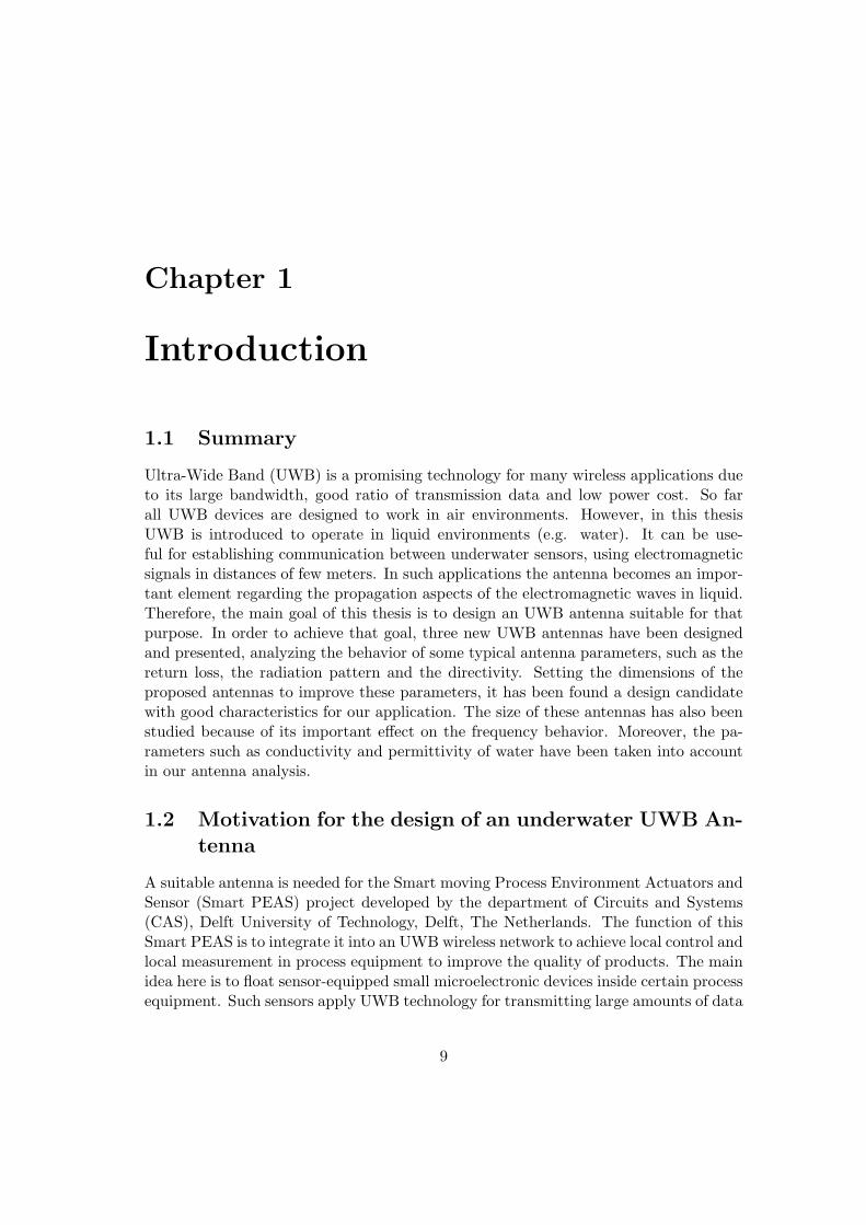
Ultra-Wide Band (UWB) is a promising technology for many wireless applications dueto its large bandwidth, good ratio of transmission data and low power cost. So farall UWB devices are designed to work in air environments. However, in this thesisUWB is introduced to operate in liquid environments (e.g. water). It can be use-ful for establishing communication between underwater sensors, using electromagneticsignals in distances of few meters. In such applications the antenna becomes an impor-tant element regarding the propagation aspects of the electromagnetic waves in liquid.Therefore, the main goal of this thesis is to design an UWB antenna suitable for thatpurpose. In order to achieve that goal, three new UWB antennas have been designedand presented, analyzing the behavior of some typical antenna parameters, such as thereturn loss, the radiation pattern and the directivity. Setting the dimensions of theproposed antennas to improve these parameters, it has been found a design candidatewith good characteristics for our application. The size of these antennas has also beenstudied because of its important effect on the frequency behavior. Moreover, the pa-rameters such as conductivity and permittivity of water have been taken into accountin our antenna analysis.
1.2 Motivation for the design of an underwater UWB An-tenna
A suitable antenna is needed for the Smart moving Process Environment Actuators andSensor (Smart PEAS) project developed by the department of Circuits and Systems(CAS), Delft University of Technology, Delft, The Netherlands. The function of thisSmart PEAS is to integrate it into an UWB wireless network to achieve local control andlocal measurement in process equipment to improve the quality of products. The mainidea here is to float sensor-equipped small microelectronic devices inside certain processequipment. Such sensors apply UWB technology for transmitting large amounts of data
9

with very low power over relative short distances. The proper hydrodynamic designof sensors with respect to size, density, robustness and fluid compatibility enables thespatial and temporal monitoring of process variables all over the vessel. The actuationfunction may as well be integrated into these devices, enabling the dynamic control ofdifferent process variables.
Another motivation for the design of an underwater UWB antenna is the limitedwork in that kind of antennas. There are a lot of designs for UWB antennas, but mostof them are done for air communications. It is needed an UWB technology to obtain agood resolution for the positioning of the devices. Furthermore, there are few studies ofelectromagnetic waves in water, but they have been done with narrow band antennas,such as dipoles or loops isolated with plastics. Hence the design of this antenna isa new challenge with a lot of possible solutions. In addition, the specifications forour application do not allow us to make a device bigger than 5cm of radius. Thisrestriction in size means an extra difficulty for finding a correct antenna, mainly witha good behavior in low frequencies.
On the other hand, the propagation of electromagnetic waves in water is very dif-ferent than in the air, because of its high dielectric constant. Actually, the attenuationis much higher in water, causing a limitation on the transmission distance. However,the main problem caused by it is the variation of the impedance of the antenna. Thischange implies a completely variation in the return loss of the antenna when it is placedin water, increasing the difficulty of the challenge.
1.3 Objectives of the thesis
The main goal of this work is to design an UWB antenna for underwater communi-cations and its applications. One of these applications is the Smart-PEAS project,explained above. This antenna will be integrated into these sensors in order to allowthe communication between them when they are placed in liquid. Our antenna has tomeet some characteristics required for this project:
• The antenna has to work between 100MHz and 1GHz because an UWB behaviouris needed.
• It is also requested a transmission in frequencies as low as possible, because therethe attenuation is less than in high frequencies.
• The antenna has to be omnidirectional because it will be placed in a device whichwill be moving.
• The size of the antenna has to be small (e.g. r ≤ 5cm).
In addition, after finding a good design for the application, the antenna will bestudied and analyzed in order to understand its behavior in different conditions. Thesestudies will be carried out varying the parameters of the antenna, and also some char-acteristics of the propagation medium, such as the conductivity and the permittivity.
10

The goal is to find out what are the environmental conditions under which the antennacan work properly.
1.4 Organization of the thesis
This report is divided into eight chapters.Chapter 2 provides an overview of Ultra-Wide Band (UWB) characteristics, prop-
erties of underwater propagation and classes of suitable antennas for our application.The chapter explain the fundamental antenna parameters and antenna requirements.
In chapter 3 two different softwares (Feko and Cst Microwave Studio 5) are com-pared to find the the most suitable for underwater applications.
Chapter 4 is dealing with the analysis of the antenna and the variations in themedium. First, some basic antennas are analyzed to find the most suitable shapes.Then, three new antennas are proposed, studying their parameters in order to achievethe antenna requirements. After that, the transmission loss between two antennasplaced in water is analyzed. Finally, an analysis of the medium properties variations ispresented.
In chapter 5 some conclusions and recommendations for future work are presented.
11

Chapter 2
Background
2.1 UWB Technology
As defined by the Federal Communications Commission (FCC), UWB technology is totransmit and receive information over a large bandwidth [9]. UWB implementationsmodulate an extremely short duration impulse that has a very sharp rise and fall time,thus resulting in a waveform that occupies several GHz of bandwidth (Fig. 2.1 andFig. 2.2).
Figure 2.1: UWB transmission with pulses
These are the two conditions of UWB technology:
BW ≥ 500MHz (2.1)
or
BW
fc≥ 0.2 (2.2)
where fc is the central frequency and BW is the bandwidth.UWB can operate between 3.1 and 10.6 GHz at limited transmission powers for
indoor communications, as defined in FCC [9]. However, for our purpose, the systemwill work between 100 MHz and 1 GHz because the propagation will be in liquid and itwon’t interfere in other technologies that use this range of frequencies in air. Generally,
12

imaging and radar implementations of UWB transmit between 1 and 100 megapulsesper second, while communications systems have between 1 and 2 gigapulses per second[1] (Fig. 2.1).
UWB was originally developed for military communications and radar. However,thanks to the good features offered, the commercial applications are increasing andUWB systems received more and more attention in the latest years.
In our application, it is needed an UWB behavior because a good resolution timeis requested (and it is inversely proportional of the bandwidth). The receiver recognizethe multipaths according to the resolution, and for the correct positioning of the devicesthis is very important.
2.1.1 UWB Advantages
Among others, we can identify the following advantages [14]:
• Possibility of high data rates.
• High resolution localization, due to the very short pulse duration.
• Channel fading resistant, due to the large number of resolvable multipath com-ponents.
• Carrier-less signal propagation.
• Overlay with existing frequency allocation, due to the low power spectral density(Fig. 2.2).
• Multiple-access capabilities, due to the wide bandwidth of transmission.
• Propagation through solid materials, due to the presence of energy at differentfrequencies.
• Possibility of coverting communications, with low probability of interception, dueto the low power spectral density.
• Simplicity in implementation, low cost of devices.
2.1.2 UWB Applications
A combination of the UWB advantages allows some interesting applications [14]:
• High Resolution Radar. It is one of the first UWB applications, because of the finepositioning characteristics of narrow pulses. They can offer a very high resolutionradar.
13

Figure 2.2: UWB and other technologies
• Wireless Personal Area Networks (WPAN). UWB is an ideal technology to replacethe wires of the personal computers and their peripherals, without interfering withyour local wireless network.
• Wireless Body Area Network (WBAN). It consists on a set of autonomous wirelesssensors with ultra-low-power requirements spread over the human body or evenimplanted inside the body.
• Sensor Networks. Networks with sensors placed inside an area or volume. Low-cost and long-life battery-operated devices are very important requirements forthis application.
• Location aware communications. The good performance of UWB devices in multi-path channels can provide accurate geolocation capability for indoor and obscuredenvironments where GPS does not work.
• Military communications. The probability to detect or intercept UWB pulses arevery low. Thus, the covert military communications are ideal for that purpose.
• Imaging systems, like ocean imaging, medical diagnostic and surveillance devices.UWB reflections of the target exhibit not only changes in amplitude and timeshift, but also changes in the pulse shape.
• Vehicular radar systems. Detection of the position and movement of objects nearthe vehicle are more accurate thanks to UWB devices.
• Emergency Situations. UWB signals can penetrate obstacles because of the widefrequency spectrum. This property is very useful to detect and rescue survivorsunder rubble in disaster situations.
2.2 Signal Propagation in Water
The most used waves to establish underwater wireless communications are the acousticwaves. However, acoustic communications are limited by two factors: low speed of
14

sound underwater and time-varying multipath propagation. Together, these factorsresult in a communication channel of poor quality and high latency. Optical systemsare another alternative to take into account, but they usually fail because of suspendedmatter of the liquid medium.
There are many applications that need a fast communication between two or moredevices within short distances. In this case, it is better to use electromagnetic wavesbecause their properties are more suitable. To study the positioning of the sensors,the system has to work fast because the position of sensors could change very fastas well, and with the acoustic waves we could make a lot of mistakes causing slowpropagation. In fact, Maxwell’s equations give us the speed of electromagnetic wavesin a medium. While for acoustic waves this speed of propagation is over 1440 m/sin water, for electromagnetic waves this propagation works over 33.5 × 10⁶ m/s (2.3),becoming more than 23× 103 times faster.
v =1√εµ
(2.3)
where v is the speed of electromagnetic propagation in a medium, µ is the permeabil-ity (in water is 1.256×10⁻⁶N/A2) and ε is the permittivity (in water is 707×10−12F/m).Note that the electromagnetic propagation in water is only about 9 times slower thanin free space. This has important advantages for command latency and networking pro-tocols in underwater communications, where information has to be exchanged betweendifferent sensors [2].
In addition, Doppler shift is inversely proportional to propagation velocity, so it ismuch smaller for electromagnetic signals:
4f = −fvrel
c(2.4)
where f is the transmitted frequency, vrel is the velocity of the transmitter relative tothe receiver in meters per second (negative when moving towards one another, positivewhen moving away) and c is the speed of wave (e.g. 33.5×10⁶ m/s for electromagneticwaves traveling in water).
2.2.1 Conductivity
The conductivity of water is dependent on its concentration of dissolved salts and otherchemical species which tend to ionize in the solution. The purer the water is, the lowerthe conductivity will be (the higher the resistivity will be). The conductivity is alsodependant on the temperature, as Table 2.1 shows [14].
These are the typical values of water conductivity [17]:
• Ultra pure water: 5.5× 10⁻⁶ S/m
• Distilled water: 0.001 S/m
• Drinking water: 0.005− 0.05 S/m
15

Table 2.1: Electrical conductivity (S/m) of sea waterTemperature (C) Salinity (g/Kg)
20 30 400 1.745 2.523 3.2855 2.015 2.909 3.77810 2.300 3.313 4.29715 2.595 3.735 4.83720 2.901 4.171 5.39725 3.217 4.621 5.974
• Sea water: 4− 5.3 S/m
• Great Salt Lake, USA: 15.8 S/m
2.2.2 Permittivity
With a relative dielectric permittivity (εr) of 81 at 20C of temperature and at 1GHz offrequency [15], water has among the highest permittivity of any material and this has asignificant impact in the behavior of the electromagnetic waves propagation. However,this value experiences variations with the frequency and the temperature. Figure 2.3shows the dielectric constant in dependance of the frequency and the temperature.The arrows show the effect of increasing temperature or increasing water activity. [18].The wavelength range 0.01 - 100cm is equivalent to 3THz - 0.3GHz respectively. Thepurpose of this section is to study the permittivity in a range between 10MHz and1GHz. As it can be noticed, for that range the dielectric constant does not vary withthe frequency. Hence it can be assumed a constat εwater of 81 when the temperatureis about 20C and the frequency is less than 1GHz.
Figure 2.3: Dielectric permittivity and dielectric loss of water between 0C and 100C
16

The permittivity in water is dependant on this relative permittivity (εr), the per-mittivity of the vacuum (εo = 8.85× 10⁻¹²) and the conductivity (σ), as the equation(2.5) shows:
εwater = εoεr − jσ
ω(2.5)
If the imaginary component appeared due to the conductivity is not taken intoaccount, and we take a relative permittivity of 81, the permittivity in water is 707 ×10−12 F/m.
2.2.3 Propagation
As far as we know, the electromagnetic propagation through water is very different frompropagation through air because water has high permittivity and electrical conductivity.
Maxwells equations are very important to predict the propagation of electromag-netic waves traveling into water. A linearly polarized plane electromagnetic wave prop-agating in the z direction may be described in terms of the electric field strength Ex
and the magnetic field strength Hy with [3]:
Ex = Eo exp(jωt− γz) (2.6)
Hy = Ho exp(jωt− γz) (2.7)
where Eo is the original electric field and Ho is the original magnetic field. Thepropagation constant γ is expressed in terms of the permittivity ε, permeability µ andconductivity σ by:
γ = jω
√εµ− j σµ
ω= α+ jβ (2.8)
where α is the attenuation factor, β is the phase factor, and ω is the angularfrequency (ω = 2πf). The term εµ arises from the displacement current and theterm σµ/ω from conduction current. It is convenient to consider the solutions for theconduction band σ/ω > ε and the dielectric band σ/ω < ε.
Investigations of the parameters σ and ε over the full electromagnetic frequencyspectrum have been obtained in electrolytic solutions by using a wide variety of exper-imental techniques [3].
In the conduction band, plane wave attenuation in water is highly compared to air,and increases rapidly with frequency [4]:
α = 0.0173√fσ (2.9)
where α is the attenuation in dB/m, f is the frequency in Hz and σ is the conduc-tivity in S/m.
If we have pure water (σ=0), we are in the dielectric band, where the attenuationis less than 10dB/m at frequencies lower than 1GHz.
17

2.2.4 Wavelength
Knowing the relationship between the wavelength λ, the speed v and frequency f as(2.10)) shows:
λ =v
f(2.10)
and with (2.1) which shows the value of speed in the water, we get that the frequencyunder water is about 9 times lower than in free space:
fwater ≈fair
9(2.11)
2.2.5 Intrinsic Impedance
In addition, the intrinsic impedance, η,(2.12) changes too. For a region with slightlyelectrical conductivity (σ > 0, e.g. seawater), the impedance is given by (2.13), andin a region with no conductivity (σ = 0, e.g. free space), the impedance simplifies to(2.14). In pure water the equation simplifies to (2.15):
η =E
H(2.12)
η =
√jωµ
σ + jωε(2.13)
ηfreespace =√µ
ε≈ 377Ω (2.14)
ηpurewater =√µpurewater
εpurewater≈ 42Ω (2.15)
In addition, Figure 2.4 shows the absolute value of the intrinsic impedance at fourdifferent frequencies (50MHz, 100MHz, 150MHz and 200MHz) in water with differentconductivities. It is observable that the impedance decreases with the conductivity,but increases with the frequency.
It can be also observed the real part and the imaginary part in Figure 2.5.
18

Figure 2.4: Intrinsic impedance on dependance of the conductivity of different frequen-cies in MHz
(a) Real part
(b) Imaginary part
Figure 2.5: Real part and imaginary part of the intrinsic impedance on dependance ofthe conductivity of different frequencies in MHz
19

2.3 Basic Antenna Parameters
A background of the fundamental antenna parameters is presented in order to under-stand the physical behavior of the antenna and also to improve its performance. Theseantenna parameters are directly obtained by a professional electromagnetic solver (CSTMicrowave Studio 5 or FEKO)[11].
2.3.1 Return loss
In a transmission line, when an incident wave propagates along it, V +, a fraction of thevoltage amplitude is reflected, V − due to the impedance discontinuities. The reflectioncoefficient, Γ, is defined as:
Γ =V −
V +=ZL − ZS
ZL + ZS(2.16)
where ZL is the impedance towards the load and ZS is the impedance towards thesource.
In our case we have a single pair of input/output terminals, referred to one port. Thecorresponding scattering matrix consists on a single element, the scattering parameteror reflection coefficient S11 [12].
b1 = S11 × a1 (2.17)
where a1 is the incident wave in the port and b1 is the reflected wave in the port.The return loss of an antenna (RL) is calculated by:
RL = −10 log10 |S11|2 = −10 log10 |Γ|2 (2.18)
Figure 2.6: Simple circuit configuration showing the ports location
2.3.2 Radiation Pattern
The antenna radiation pattern is defined as the spatial distribution of a quantity whichcharacterizes the electromagnetic field generated by an antenna [13]. It is possible torepresent the radiation pattern of an antenna using three dimensions or two dimensions,
20

on both spherical and polar coordinate systems respectively. The two dimensional ra-diation pattern can be used to determine the relative strength of the radiation powerin the far field with regard to the direction. On the spherical coordinate system twodifferent planes are particulary interesting: the E-plane (the plane containing the elec-tric field vector and the direction of maximum radiation) and the H-plane (the planecontaining the magnetic field vector and the direction of maximum radiation)
Figure 2.7: E-plane and H-plane for a dipole antenna
In this thesis we are going to study the gain. The level of this parameter is relatedwith the power of the feeding. With the directivity, it allows to know the efficiency ofthe antenna.
2.3.3 Directivity
The directivity in a direction measures the power density that an antenna radiates in aspecific direction, relative to the power density radiated by an ideal isotropic radiatorantenna radiating the same amount of total power.
This parameter is related with the power of radiation, and it is used to know theefficiency of the antenna with the equation (2.19).
G = N ×D (2.19)
where G is the gain, D is the directivity, and N is the efficiency of the antenna.
2.4 Underwater Antennas
The main goal of the project is designing an antenna for UWB underwater communica-tions. But first we have to know which antennas are more suitable for propagation intowater. Published references [5] indicate that loop antennas, long wires and dipoles havebeen successfully used underwater at very low frequencies. Because of the reduction ofthe frequency shown in the equation (2.11), their physical dimensions are lower thantheir equivalent in space.
21

(a) Circular loops (b) Folded dipole
Figure 2.8: Different classes of underwater antennas
Historically, in the underwater communications, antenna conductors are insulatedfrom the water to prevent leakage of direct current to the conducting medium. But thisis not our goal. We are going to design a small antenna with the conductors directlytouching water because of the small size required [1].
2.5 UWB Antennas
There are three different classes of UWB antennas based on different applications [8]:
DC-to-daylight: These antennas are designed to have maximum bandwidth and touse as much spectrum as possible. Typical applications are ground penetratingradars, field measurements or electromagnetic compatibility, impulse radars, andshelter communication systems.
Multi-narrowband: The design goal of multi-narrow band antennas is similarly tograb as much spectrum as possible but to only use small sub-bands at any giventime. These antennas are designed as scanner or signal intelligence antenna forreceiving or detecting relatively narrowband signals through certain frequencies.
Modern: These are antennas designed for use in conjunction with the approximately3:1 bandwidth, as 3.1-10.6 GHz UWB systems authorized by the FCC (FederalCommunications Commission). The bandwidth requirements for a modern UWBantenna are narrower than for DC to daylight antennas. These antennas havecertain implication that distinguish them from the other more traditional classesof UWB antennas. First, instead of trying to grab maximal bandwidth, thesemodern UWB antennas must operate within a certain spectral mask. In this con-text, excessive bandwidth degrades system response and is counterproductive.
22

Second, unlike multi-narrowband antenna, a modern UWB antenna potentiallyuses much, if not all, of its bandwidth at the same time. Thus, a modern UWBantenna must be well behaved and consistent across the antennas operationalband. Its properties include radiation pattern, gain, antenna matching, and re-quirement for low or no dispersion. A wide variety of antennas meets the demandsof modern UWB system.
(a) Bow-tie (b) Spiral
(c) Horn
Figure 2.9: Different classes of UWB antennas
Otherwise, the antennas for UWB technology can be divided into the followinggroup based on the characteristics [8]:
Frequency independent antennas: Antennas whose mechanical dimensions are shortcompared to the operating wavelength are usually characterized by low radiationresistance and large reactance. This combination results in a high quality leveland consequently a narrow bandwidth. The current distribution on a short con-ductor is ideally sinusoidal with zero current at the free end, but because theconductor is so short electrically, typically less than 30 of a sine wave, the cur-rent distribution will be approximately linear. By end loading to give a constantcurrent distribution, the radiation resistance is increased four times, thus greatlyimproving the efficiency but not noticeably altering the pattern. Because theeffective source of the radiated fields varies with frequency, these antennas tendto be dispersive. Examples of frequency-independent antennas include spiral, logperiodic, and conical spiral antennas.
Horn antennas: A horn antenna is an electromagnetic funnel concentrating energyin a particular direction. Horn antennas tend to have high gain and relativelynarrow beams. Horn antennas also tend to be large and bulkier than small-element antennas. These antennas are well suited for point-to-point links or
23

other applications where a narrow field of view is desired. As an example we canmention the TEM (Transverse Electromagnetic mode) horn antenna.
Reflector antennas: A reflector antenna also concentrates energy in a particular di-rection. Like horn antennas, reflector antennas tend to have high gain and arerelatively large. Reflector antennas tend to be structurally simpler than horn an-tennas and are easier to be modified and adjusted by manipulating the antennafeed.
Small element antennas: These antennas tend to be small, omnidirectional anten-nas well suited for commercial applications. Examples of small element antennasinclude Lodges biconical and bow-tie antennas, diamond dipole, ellipsoidal an-tennas, and Thomass circular dipole.
2.6 Antenna Design Requirements
To design our specific antenna, the parameters described in Section 2.3 should be takeninto account, and the final shape should satisfy different specifications such as physicalsize and electrical performance.
• As far as the electrical performance is concerned, the antenna should be ableto transmit a pulse having a bandwidth (|S11| ≤-10 dB) located in the rangefrom 100 MHz to 1 GHz (wide bandwidth implies a good resolution time). Areturn loss level lower than -10 dB means that more than the 90% of the energyis radiated.
• The omnidirectionality of the antenna is another important requirement, becausethis antenna should transmit in all directions, thus the radiation pattern shouldbe as much omnidirectional as possible.
• The size is another important factor in this project, because the final applicationrequires a small antenna with a diameter around 5-10 cm. This restriction is thehardest specification due to the relationship between the size and the frequency.For lower frequencies as required in the specifications, the size should be bigger.Thus, the design of a small antenna becomes a challenging issue.
24
Chapter 3
Tools for Underwater AntennaSimulations
Usually, antenna designers use some kind of software to simulate the response of theantennas to be able to analyze the results and to determine the best shape for eachapplication. However, these applications are normally for air, and the simulation toolsof these softwares are prepared for that purpose and not for underwater applications. Ithas been tested two of the most used softwares (FEKO and CST Microwave Studio 5)in different conditions to determine which one is the best for underwater applications.
First, we analyze the differences between both softwares. We explain the reasonbecause FEKO is better than CST when simulating antennas in water. Second wesimulate a dipole with FEKO and with CST to be able to check the differences. Finally,we give some conclusions about the behavior of each software.
3.1 Software Characteristics
In this section we give an overview of the most interesting differences of the simula-tion tools between both softwares (FEKO and CST Microwave Studio 5). There aremore interesting tools. However, by analyzing these characteristics, we will be able todetermine which one is the best software for the applications in mediums with a highpermittivity.
3.1.1 The Mesh
Both softwares are very good for simulations in air. However, the high permittivityof the water makes the simulations more difficult. Each software uses a different wayto solve the simulations, and it depends basically of the mesh used to determine theantenna’s area or volume of interest. Each software is more suitable depending on theapplication.
In the application that we study, we need simulations in water with a permittivityof 81. That means that we need a dense mesh to obtain good results. Nevertheless, if
25

the mesh is too dense, the software is not able to solve the simulation. The choice ofthe correct mesh is one of the most important and hard decisions.
In CST software, the mesh is three-dimensional. The solver takes a determinatevolume of the background where the shape is placed, and analyzes all the volume withthe mesh. The shape of the mesh cells is rectangular (Figure 3.1a). In order to choosean appropriate mesh in CST, we have to modify some parameters:
Lines per wavelength This value is connected to the wavelength of the highest fre-quency set for the simulation. It defines the minimum number of mesh lines ineach coordinate direction that are used for a distance equal to this wavelength.In a way, it sets the spatial sampling rate for the signals inside of your structure.This setting has a strong influence on the quality of the results and on the calcu-lation time. Increasing this number leads to a higher accuracy, but unfortunatelyalso increases the total calculation time.
Refine at PEC / lossy metal edges by factor This option increases the spatialsampling at PEC (Perfect Electric Conductor)or lossy metal edges. At theseedges additional density points are added that force the automatic mesh genera-tor to increase the mesh density at those points by the given factor. This settingis very useful, because at metal edges you theoretically obtain singularities inthe electromagnetic fields. This means, that the fields vary very much near suchedges and have to be sampled higher than elsewhere.
(a) CST (b) FEKO
Figure 3.1: Different meshes
Otherwise, FEKO software works in a different way. The solver only takes thesurface or volume needed, but not the background. The shape of the cells is triangular(Figure 3.1b). To choose a correct mesh in FEKO, we have to determine the size of thecells. We can try a bigger size for the big faces of the shape, but we should choose asmall size for other faces and for the edges, because there are more singularities in theelectromagnetic fields, and they have big variations.
When working into water, a weighty mesh is needed due to the high permittivity.Thus, the software more suitable is FEKO, because the number of cells needed is lower(that means less execution time in simulations), and also the triangular shape gives us
26
a better precision. Moreover, FEKO shows warnings and errors more accurately thanin CST.
3.1.2 The Background Properties
In CST Microwave studio 5 we do not have the opportunity to change more parametersthan the relative permittivity (εr). Otherwise, in FEKO we can change more param-eters, such as the conductivity (σ) or the dielectric loss factor (tan δ) , which have adirect effect in the permittivity (ε) (eq. 3.1 and 3.2).
ε = εoεr − jσ
ω(3.1)
ε = εoεr(1− j tan δ) (3.2)
Both parameters depend on the kind of water used. However, we are not going toanalyze these parameters now.
In the next chapter an analysis of the dipole’s behavior is shown in order to checkif there are more differences between FEKO and CST.
3.2 Analysis of a Dipole Antenna
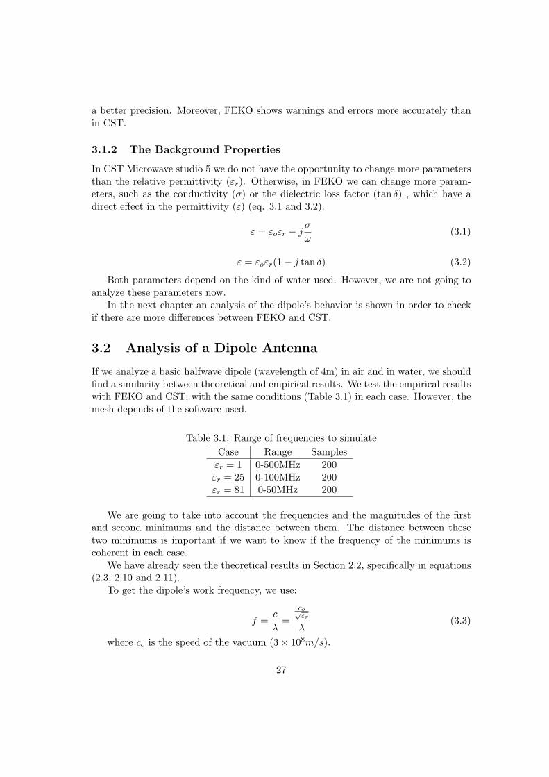
If we analyze a basic halfwave dipole (wavelength of 4m) in air and in water, we shouldfind a similarity between theoretical and empirical results. We test the empirical resultswith FEKO and CST, with the same conditions (Table 3.1) in each case. However, themesh depends of the software used.
Table 3.1: Range of frequencies to simulateCase Range Samplesεr = 1 0-500MHz 200εr = 25 0-100MHz 200εr = 81 0-50MHz 200
We are going to take into account the frequencies and the magnitudes of the firstand second minimums and the distance between them. The distance between thesetwo minimums is important if we want to know if the frequency of the minimums iscoherent in each case.
We have already seen the theoretical results in Section 2.2, specifically in equations(2.3, 2.10 and 2.11).
To get the dipole’s work frequency, we use:
f =c
λ=
co√εr
λ(3.3)
where co is the speed of the vacuum (3× 10⁸m/s).
27

3.2.1 Case 1: εr = 1 (Air)
First of all, we analyze the behavior of the return loss of the dipole in air (Figure 3.2).In FEKO, we obtain that the antenna is matched around 71.2MHz, while the the-
oretical result is 75MHz (equation 3.3). The next frequency with a minimum returnloss is 221.7MHz. Hence, the distance between both frequencies is 165MHz.
In CST, the antenna is matched at 73.7MHz, and the next minimum is in 221.7MHz.The distance is 148MHz.
Both graphics are very similar in low frequencies, but the third minimum is notexactly the same. We can also see that the level of the first minimum is better (lower)in FEKO than in CST.
Figure 3.2: S11 of a dipole in air
3.2.2 Case 2: εr = 25
If we apply the equation 3.3 in this case, we obtain that the work frequency is 15MHz.Figure 3.3 shows us that both simulations are very similar. The first minimum is
at 15.4MHz, and the second one is at 45.7MHz. The difference is 30.3MHz. However,the first frequency matched is located in the third minimum, at 77MHz. Hence we seethat the impedance has changed.
Due to the theory, we know the frequencies should be the same in this case, butdivided by
√εr when we change the background. Thus, taking the difference between
the two minimums in air, the new differences should be 29.6MHz in CST (148/√
25)and 30.1MHz (150.5/
√25). These values are close to the empirical result of 30.3MHz
found in the simulations.
28

Figure 3.3: S11 of a dipole in a background with a relative permittivity of 25
3.2.3 Case 3: εr = 81 (Water)
Finally, we put the dipole in water (εr of 81). From (3.3) we know that the workfrequency is 8.3MHz.
Figure 3.4: S11 of a dipole in water
Figure 3.4 shows us the simulation. In FEKO the first minimum is at 11.1MHz,while the second one is at 28MHz. The separation between them is 16.9MHz, close tothe 16.7MHz theoretically obtained (150.5/
√81).
In the CST simulation, the first minimum is at 11.6MHz, and the second one at28.3MHz. The difference is exactly 16.7MHz, as the theory indicates.
The frequencies are close to the theory in both softwares, but the level of the |S11|is very different. If we try to improve the mesh, we obtain the same results in FEKO,and in CST the level approaching to the FEKO’s one.
29

3.3 Conclusions
Table 3.2 compares the results between FEKO and CST.
Table 3.2: Results of the simulations (in MHz)Case Theory CST FEKOεr = 1 75 73.7 71.2εr = 25 15 15.4 15.4εr = 81 8.3 11.6 11.1
It can be concluded that the results of the simulations are similar to the results ofthe equations. However, when we increase the permittivity, the lower frequencies arenot matched. That means that the impedance in water changes, and we have to solveit by improving the parameters of the shape.
Furthermore, it is interesting to know which software takes more time to run thesimulations, because when the permittivity is very high, the time of the simulationsincreases. The Table 3.3 shows the time of the simulations.
Table 3.3: Times of the simulationsCase CST FEKOεr = 1 1min 7secεr = 25 9min 10secεr = 81 35min 1min
In this table we can observe that CST delayed faster than FEKO in high permittiv-ities. These results are manageable times, but when the range of frequencies increases,the time increases too. Specially in CST software, the simulations can be delayed forseveral hours. For example, if the frequency range is from 0 to 1GHz, the simulationof the dipole in water takes more than 2 hours in CST. On the other hand, in FEKOsoftware the same simulation just takes few minutes.
To get correct results, the mesh has to be improved in each case. When the permit-tivity increases, the density of the mesh has to be increased too. In CST this operationimplies a long simulation time.
In addition, as we can see in the Figures 3.2 and 3.3, the simulations in CST havecurls in some low frequencies, but not in FEKO.
And also we have to remember Section 3.1.2, where it was told that in FEKO it ispossible to change more background parameters than CST, allowing a complete studyof the antenna behavior.
Hence, it can be finally concluded that FEKO is more suitable than CST to simulateantennas for underwater applications.
30

Chapter 4
Antenna Analysis
This chapter is dealing with the analysis of the requested antenna. First, we test somecandidate shapes that we think that could be suitable for the application. For example,the circular loop, which is usually used in underwater communications (Section 2.4),and some typical antennas used in UWB systems (Section 2.5). After that, we combinethe most suitable shapes to achieve an antenna that meets the requirements. Then, aparametric study of the dimensions is performed to find the best design.
Finally, once the antenna has been selected, we analyze the behavior of the shapewhen changing the properties of the medium.
4.1 Basic Shapes
In this section we study simple shapes in air and we will compare the obtained resultswhen the antenna is put in water. First, we consider the circular loop because it showna good behavior in water (see Section 2.4). After that, we will study some typicalUWB antennas, such as the circular dipole, the diamond and the bow-tie antenna. Wewant to test the possibility of using them in water because their response in air couldbe similar to that in water, but in a bandwidth 9 times lower, and with a differentreturn loss level (because the impedance depends of the environment, as we have seenin Section 2.3.1). Finally, we will compare all the results to choose the best shape forour application. In FEKO software we can obtain the return loss, the phase and theradiation pattern.
To study these shapes, we choose sizes close to radius of 5cm, because it is themaximum size permitted by the requirements. In air, the range of frequencies analyzedis from 10MHz to 9GHz, with 200 samples . Otherwise, because in water the frequenciesare 9 times lower, the studied range is from 10MHz to 1GHz, also with 200 samples.The reason for this choice is that the frequencies in water are 9 times lower than in air,and also we want to study the behavior in low frequencies.
The feeding in both cases do not have to touch water because it is needed a electricaldevice to feed the antenna. In the air simulations this is not a problem, but in the
31

water simulations we have to isolate the feeding. In these cases, the isolation is doneby putting the feeding inside a small region with free space.
4.1.1 Circular Loop
Figure 4.1: Dimensions of circular loop antenna
To study the behavior of the circular loop we use a circular wire with a radius of5cm (Figure 4.1). We analyze the differences between the response in air and in waterto check the viability of this shape for our purpose.
(a) in air (b) in water
Figure 4.2: S11 of circular loop
As we can observe in Figure 4.2, the return loss in air at 1GHz is above the levelof -10dB. The dimensions of the antenna are chosen just to study these two responses,both in air and in water. In water we can see that in frequencies close to 1GHz thelevel of |S11| is better.
Thus, it has been concluded that the circular loop presents a better behavior inwater environment than in air. This shape could be a good start for the design of theantenna that we are looking for the application.
4.1.2 Circular Dipole
It has been shown that a circular loop could be a good antenna, but it has to be anUWB antenna, and that is the reason why some UWB antennas in water have beenstudied.
32
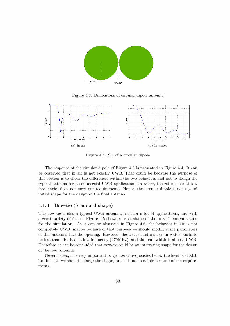
Figure 4.3: Dimensions of circular dipole antenna
(a) in air (b) in water
Figure 4.4: S11 of a circular dipole
The response of the circular dipole of Figure 4.3 is presented in Figure 4.4. It canbe observed that in air is not exactly UWB. That could be because the purpose ofthis section is to check the differences within the two behaviors and not to design thetypical antenna for a commercial UWB application. In water, the return loss at lowfrequencies does not meet our requirements. Hence, the circular dipole is not a goodinitial shape for the design of the final antenna.
4.1.3 Bow-tie (Standard shape)
The bow-tie is also a typical UWB antenna, used for a lot of applications, and witha great variety of forms. Figure 4.5 shows a basic shape of the bow-tie antenna usedfor the simulation. As it can be observed in Figure 4.6, the behavior in air is notcompletely UWB, maybe because of that purpose we should modify some parametersof this antenna, like the opening. However, the level of return loss in water starts tobe less than -10dB at a low frequency (270MHz), and the bandwidth is almost UWB.Therefore, it can be concluded that bow-tie could be an interesting shape for the designof the new antenna.
Nevertheless, it is very important to get lower frequencies below the level of -10dB.To do that, we should enlarge the shape, but it is not possible because of the require-ments.
33
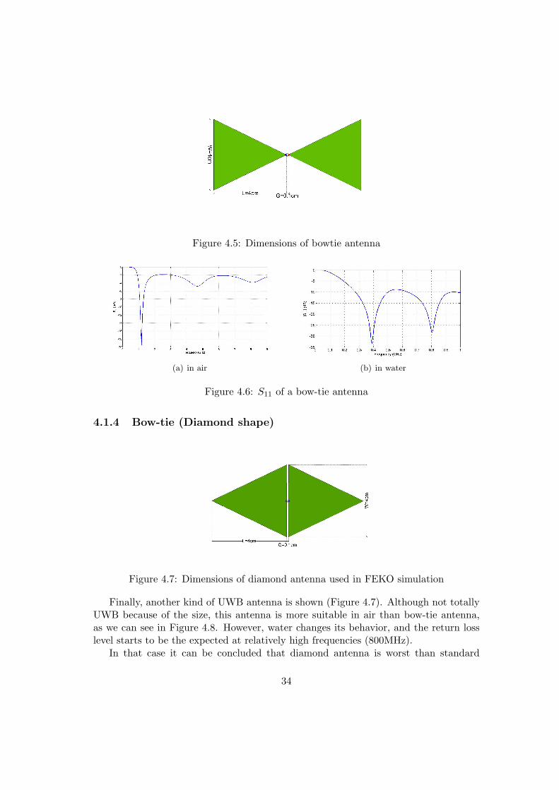
Figure 4.5: Dimensions of bowtie antenna
(a) in air (b) in water
Figure 4.6: S11 of a bow-tie antenna
4.1.4 Bow-tie (Diamond shape)
Figure 4.7: Dimensions of diamond antenna used in FEKO simulation
Finally, another kind of UWB antenna is shown (Figure 4.7). Although not totallyUWB because of the size, this antenna is more suitable in air than bow-tie antenna,as we can see in Figure 4.8. However, water changes its behavior, and the return losslevel starts to be the expected at relatively high frequencies (800MHz).
In that case it can be concluded that diamond antenna is worst than standard
34

bow-tie antenna for underwater environments.
(a) in air (b) in water
Figure 4.8: S11 of a diamond antenna
35

4.2 Folded Bow-tie Antenna: First shape
After the analysis of some typical UWB antennas, it has been concluded that circularloop and bow-tie antennas are the most suitable for the underwater application. Thecombination of both shapes may arise into a new antenna.
The simulations are done completely in FEKO, using an accurate mesh to ensurereliable results. The most important characteristics taken into account are:
• The return loss must be less than -10 dB from a low frequency around 100MHz.
• An UWB behavior is needed.
• The antenna has to be omnidirectional.
• The size of the shape cannot measure more than 5cm of radius.
As far as we know, the application uses small devices to work. Hence the antennasize has to be as smaller as possible. This restriction is very important to determinethe low frequency from which the return loss level becomes minor than -10dB. Figure4.9 shows the dimensions of the first candidate:
(a) Perspective view (b) Top wiew
Figure 4.9: First candidate: original antenna dimensions
The gap feeding is 1cm because it is not isolated yet. In the parametric analysis ofthe next sections we will isolate the feeding and we will check the best measure.
The results of the FEKO’s simulation indicates:
1. The return loss is less than -10dB from 150MHz (Figure 4.10).
2. The behavior is UWB because the bandwidth is greater than 500MHz (Figure4.10).
4.2.1 Parametric study
The parametric study of the first candidate is presented, for which the parameters tobe analyzed are:
36

Figure 4.10: S11 of original first candidate
• Angle (α)
• Width (W)
• Thickness (T)
• Feeding (G)
• Size (R)
The original parameters are shown in Figure 4.9. These original values have beentaken because they are similar of the typical bow-tie and loop parameters. Variationsof each parameter are compared to the original one. Finally, the most suitable antennawill be found.
Angle
First, we check if the original angle (α = 30) has the best response.As it can be seen in Figure 4.11a, there is another opening angle better than the
original. In fact, an angle of α = 20 implicates a return loss level lower than with anangle of α = 30. Notice that this angle is the minimum possible for this shape, thusis not possible to choose an angle less than α = 20 because the width would have tobe changed. In a new section some angles will be studied changing the width.
Width
In this section the width of the shape is studied. The original one has a width of 1.6cm.However, as it can be seen in Figure 4.11b, a width of 2.4cm is better.The results of the parametric study of the angle and the width lead us to think that
it is possible to improve the return loss changing the width an the angle at the same
37

(a) Angle (b) Width
Figure 4.11: |S11| of the first candidate changing some parameter
time. The best combination occurs when the cut from the feeding finishes in the halfof the antenna.
Figure 4.12: |S11| with different widths and angles
Hence, these five combinations are tested:
• Width=0.8cm. Angle=5
• Width=1.6cm. Angle=10
• Width=2.4cm. Angle=15
• Width=3.2cm. Angle=20
• Width=4cm. Angle=25
Figure 4.12 shows the combinations within the width and the opening angle. Itis possible to observe that there are two options better than the others: the width of1.6cm and the width of 2.4cm. To discern the best option, we take the antenna with
38
a width of 2.4cm and the angle of α = 30 because it starts to have lower frequenciesbelow -10dB before than the other candidate.
Thickness
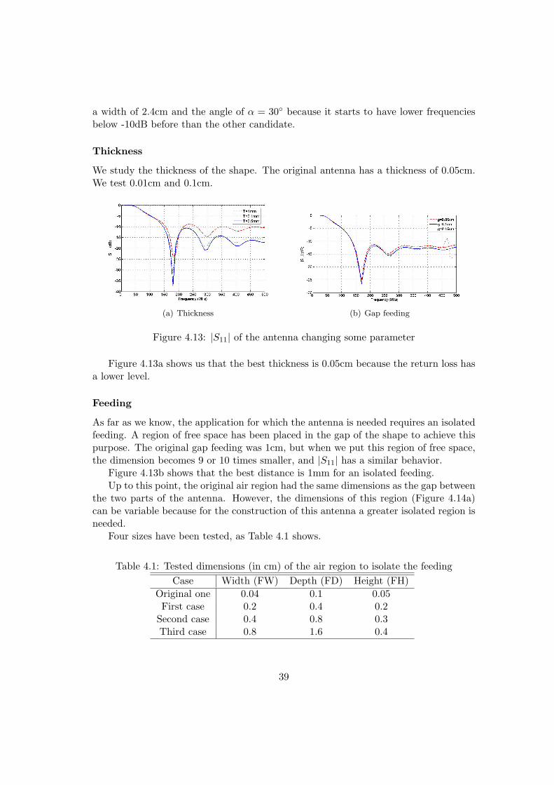
We study the thickness of the shape. The original antenna has a thickness of 0.05cm.We test 0.01cm and 0.1cm.
(a) Thickness (b) Gap feeding
Figure 4.13: |S11| of the antenna changing some parameter
Figure 4.13a shows us that the best thickness is 0.05cm because the return loss hasa lower level.
Feeding
As far as we know, the application for which the antenna is needed requires an isolatedfeeding. A region of free space has been placed in the gap of the shape to achieve thispurpose. The original gap feeding was 1cm, but when we put this region of free space,the dimension becomes 9 or 10 times smaller, and |S11| has a similar behavior.
Figure 4.13b shows that the best distance is 1mm for an isolated feeding.Up to this point, the original air region had the same dimensions as the gap between
the two parts of the antenna. However, the dimensions of this region (Figure 4.14a)can be variable because for the construction of this antenna a greater isolated region isneeded.
Four sizes have been tested, as Table 4.1 shows.
Table 4.1: Tested dimensions (in cm) of the air region to isolate the feedingCase Width (FW) Depth (FD) Height (FH)
Original one 0.04 0.1 0.05First case 0.2 0.4 0.2
Second case 0.4 0.8 0.3Third case 0.8 1.6 0.4
39
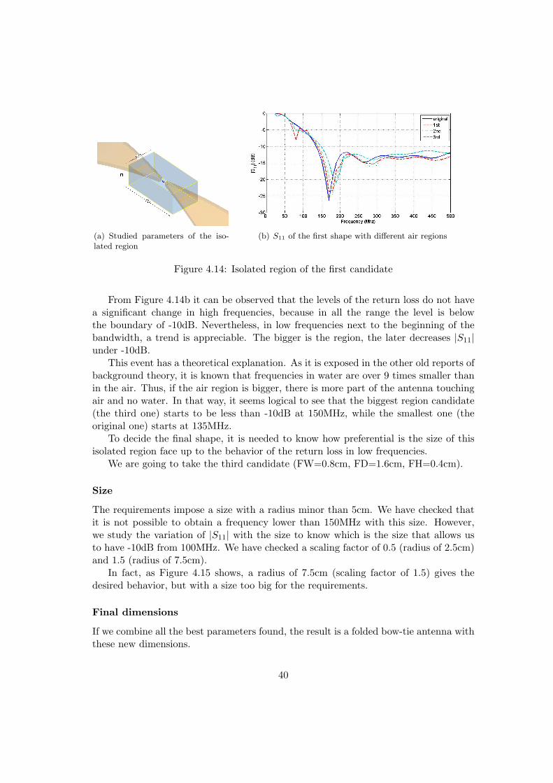
(a) Studied parameters of the iso-lated region
(b) S11 of the first shape with different air regions
Figure 4.14: Isolated region of the first candidate
From Figure 4.14b it can be observed that the levels of the return loss do not havea significant change in high frequencies, because in all the range the level is belowthe boundary of -10dB. Nevertheless, in low frequencies next to the beginning of thebandwidth, a trend is appreciable. The bigger is the region, the later decreases |S11|under -10dB.
This event has a theoretical explanation. As it is exposed in the other old reports ofbackground theory, it is known that frequencies in water are over 9 times smaller thanin the air. Thus, if the air region is bigger, there is more part of the antenna touchingair and no water. In that way, it seems logical to see that the biggest region candidate(the third one) starts to be less than -10dB at 150MHz, while the smallest one (theoriginal one) starts at 135MHz.
To decide the final shape, it is needed to know how preferential is the size of thisisolated region face up to the behavior of the return loss in low frequencies.
We are going to take the third candidate (FW=0.8cm, FD=1.6cm, FH=0.4cm).
Size
The requirements impose a size with a radius minor than 5cm. We have checked thatit is not possible to obtain a frequency lower than 150MHz with this size. However,we study the variation of |S11| with the size to know which is the size that allows usto have -10dB from 100MHz. We have checked a scaling factor of 0.5 (radius of 2.5cm)and 1.5 (radius of 7.5cm).
In fact, as Figure 4.15 shows, a radius of 7.5cm (scaling factor of 1.5) gives thedesired behavior, but with a size too big for the requirements.
Final dimensions
If we combine all the best parameters found, the result is a folded bow-tie antenna withthese new dimensions.
40

Figure 4.15: |S11| of the antenna with different size
(a) feeding region (b) top view
Figure 4.16: Dimensions of the final antenna
Thus, the dimensions of the new antenna are shown in Figure 4.16, the return lossin Figure 4.17, and the radiation pattern in Figure 4.18.
The results of the FEKO’s simulation indicates:
1. The return loss is less than -10dB from 135MHz (Figure 4.17) face up to the150MHz of the original shape.
2. The behavior is UWB because the bandwidth is greater than 500MHz, it is from135MHz to 1800MHz. Thus, the bandwidth is 1665MHz (Figure 4.17). Specifi-cally, the relative bandwidth is more than 0.2, the minimum required to becomeUWB:
BW
fc=
1665((1665)/2) + 135
= 1.73 > 0.2 (4.1)
41

Figure 4.17: S11 of the new antenna and the old one
(a) 151MHz (b) 292MHz
(c) 454MHz (d) 596MHz
Figure 4.18: Radiation pattern of the first candidate without internal isolation
3. The final antenna has a better return loss in low frequencies than the originalone, but in high frequencies the opposite happens. However, the low frequenciesare more important than the higher ones in the water propagation because theattenuation is lower. Thus, it is more important to have a good return loss level
42

at low frequencies.
4. The radiation pattern is almost omnidirectional (Figure 4.18). It is not totallyomnidirectional because when the length of the ring is greater than a half wavedipole, they appear some new nulls and some new lobes in the pattern. Figure4.19 helps to understand this kind of behavior: in the first case, the wavelength ismuch more greater than the length of the dipole. In the second case, the antennais a halfwave dipole (from this length they will appear a new secondary lobe). Inthe third case, the dipole has the same length as the wavelength, and the radiationpattern has two main lobes. Finally, in the fourth case, there are more secondarylobes. Thus, the higher the frequency is, more lobes the radiation pattern has.
Figure 4.19: Dipoles with different lengths related to the wavelength
4.2.2 Final shape with internal isolation
The antenna needs a battery and a circuit to work, but they cannot be touching water.Thus we have to isolate the center of the antenna with a sphere. In this section we willstudy the behavior of the antenna when an air ball or an air-teflon ball (teflon has anεr of 2.1) is placed inside the antenna, as Figure 4.20 shows.
The boundary of the air ball in the first case is touching the antenna. On theother hand, the air-teflon ball is almost the same, but with a half centimeter of teflonrecovering the air. This is important because air and water have to be, obviously,separate.
Furthermore, the air region of the feeding has to be improved. Otherwise, in theair-teflon ball case, we have added one millimeter of teflon to separate air and water(Figure 4.21b).
The behavior of the antenna is presented in the next sections.
43

(a) air ball (b) air-teflon ball
Figure 4.20: First candidate with internal isolation
(a) front view (b) zoom of the feeding zone
Figure 4.21: Materials and dimensions of first candidate with an air-teflon isolation
Return loss
As far as we know, the return loss level is one of the most important parameters totake into account. Specially a good matching in low frequencies is needed, where thepropagation in water is better. Figure 4.22 shows the |S11| results of the three modelsproposed of the first antenna candidate: the antenna without internal isolation, withan air ball, and with an air-teflon ball.
First, we check that in low frequencies the internal isolation allows the transmissionin lower frequencies (almost 100MHz), while without this isolation the return loss islower than -10dB since 135MHz. However, if we take a look at the high frequencies,the behavior is the opposite: the internal isolation reduces the transmission in highfrequencies (660MHz in case of air-teflon ball and 800Mz in case of air ball), while inthe model without any isolation ball the transmission is possible in frequencies higherthan 1GHz.
As Table 4.2 shows, the three models are UWB because the bandwidth is greaterthan 500MHz, but there is a lot of difference in the behavior of high frequencies betweenthe isolated antenna and the antenna without isolation. However, as we explainedbefore, in water the most important range of frequencies is the range of low frequencies
44
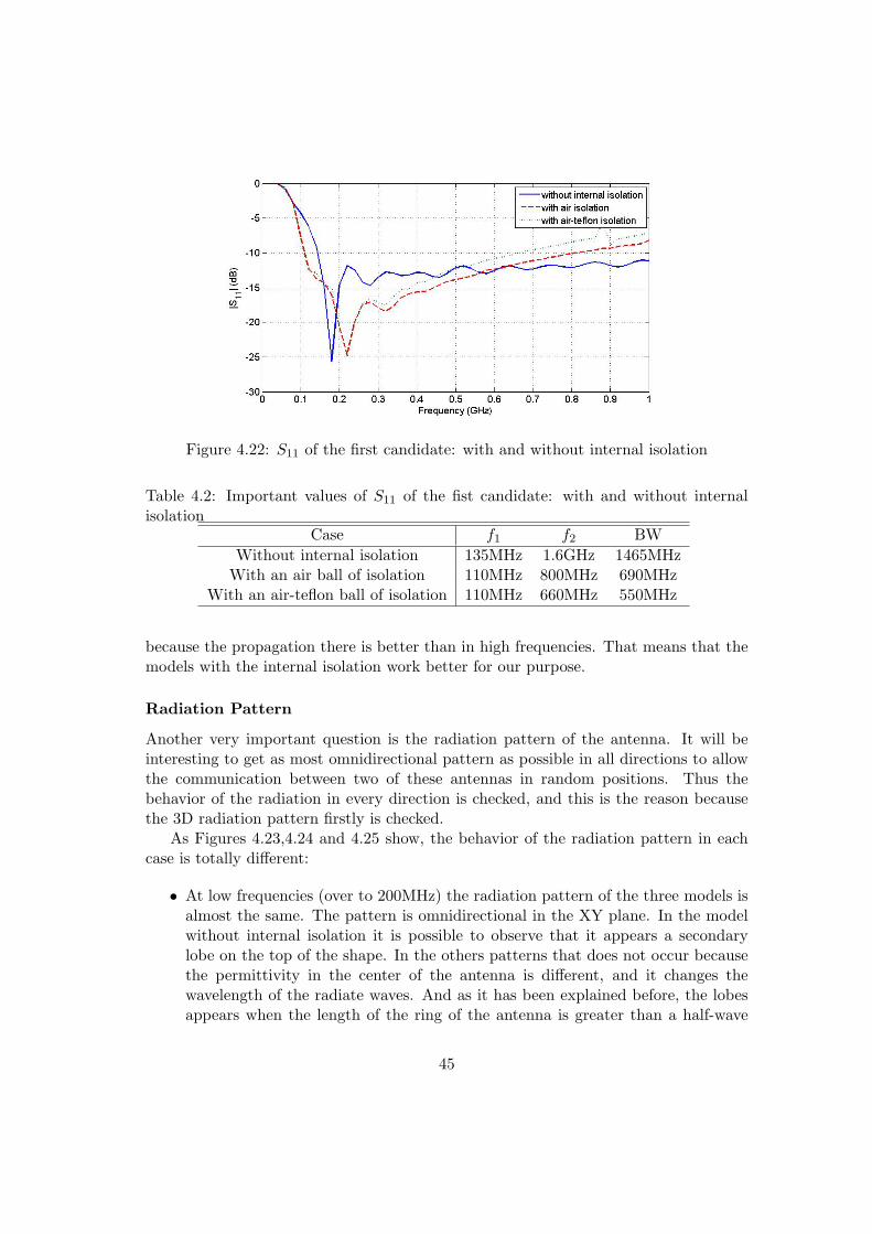
Figure 4.22: S11 of the first candidate: with and without internal isolation
Table 4.2: Important values of S11 of the fist candidate: with and without internalisolation
Case f1 f2 BWWithout internal isolation 135MHz 1.6GHz 1465MHz
With an air ball of isolation 110MHz 800MHz 690MHzWith an air-teflon ball of isolation 110MHz 660MHz 550MHz
because the propagation there is better than in high frequencies. That means that themodels with the internal isolation work better for our purpose.
Radiation Pattern
Another very important question is the radiation pattern of the antenna. It will beinteresting to get as most omnidirectional pattern as possible in all directions to allowthe communication between two of these antennas in random positions. Thus thebehavior of the radiation in every direction is checked, and this is the reason becausethe 3D radiation pattern firstly is checked.
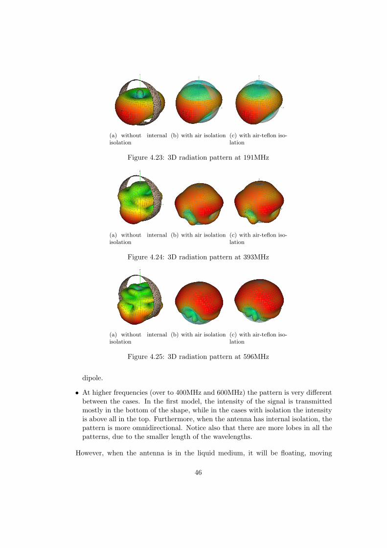
As Figures 4.23,4.24 and 4.25 show, the behavior of the radiation pattern in eachcase is totally different:
• At low frequencies (over to 200MHz) the radiation pattern of the three models isalmost the same. The pattern is omnidirectional in the XY plane. In the modelwithout internal isolation it is possible to observe that it appears a secondarylobe on the top of the shape. In the others patterns that does not occur becausethe permittivity in the center of the antenna is different, and it changes thewavelength of the radiate waves. And as it has been explained before, the lobesappears when the length of the ring of the antenna is greater than a half-wave
45
(a) without internalisolation
(b) with air isolation (c) with air-teflon iso-lation
Figure 4.23: 3D radiation pattern at 191MHz
(a) without internalisolation
(b) with air isolation (c) with air-teflon iso-lation
Figure 4.24: 3D radiation pattern at 393MHz
(a) without internalisolation
(b) with air isolation (c) with air-teflon iso-lation
Figure 4.25: 3D radiation pattern at 596MHz
dipole.
• At higher frequencies (over to 400MHz and 600MHz) the pattern is very differentbetween the cases. In the first model, the intensity of the signal is transmittedmostly in the bottom of the shape, while in the cases with isolation the intensityis above all in the top. Furthermore, when the antenna has internal isolation, thepattern is more omnidirectional. Notice also that there are more lobes in all thepatterns, due to the smaller length of the wavelengths.
However, when the antenna is in the liquid medium, it will be floating, moving
46

and rotating all the time. Thus, it can be concluded that the three models of the firstcandidate are almost omnidirectional.
(a) 151MHz (b) 292MHz
(c) 454MHz (d) 596MHz
Figure 4.26: Radiation pattern of the gain (in dB) in 2D (XZ plane) at different fre-quencies
Also the radiation pattern in two dimensions can be analyzed, specifically in themiddle of the antenna, in the XZ plane (Figure 4.26).
In this case the values of the gain in dB can be seen, in some frequencies in therange of interest. Almost in all the frequencies this value is between -10dB and 0dB.These levels related with the levels of directivity of the next section indicates that theefficiency of the antenna is not very good because the difference between the gain andthe directivity is about 3dB.
Directivity
To understand better the far field intensity of the most significantly directions, a studyof the directivity in dependance of the frequency in the top (Z direction), the middle
47

(X direction and Y direction) , and the bottom of the antenna (-Z direction); can bedone, as Figure 4.28 shows.
Figure 4.27: Spherical coordinates and points of interest
Analyzing the results for each case, it is possible to conclude that:
• The antenna without internal isolation radiates better in the middle 1 (X direc-tion) at low frequencies (from 135MHz to 250MHz), while at frequencies from250MHz it radiates with more intensity in the bottom. It can also be appreciatedthat in the top (Z direction) and in the middle 2 (Y direction) of the shape theradiation is not very appropriate because it oscillates too much.
• In the cases of air and an air-teflon isolation, the radiation is higher in the middle1 at frequencies between 100MHz and 350MHz, but from 350MHz the majordirectivity is in the top of the shape and in the middle 2.
It is also interesting to realize that almost all the levels of the directivity remainbetween -10dB and 5dB. If the radiation pattern was totally omnidirectional, the di-rectivity would be 0dB in all the directions (like a perfect sphere). Otherwise, if theradiation pattern was directional, the directivity would be more than 0dB in some di-rections and less than 0dB in the rest of the pattern. Hence it can be concluded that thedirectivity of this antenna is different in each case and in each direction. Nevertheless,because of the continuous movement of the device where the antenna will be placed,the behavior is quite correct.
48
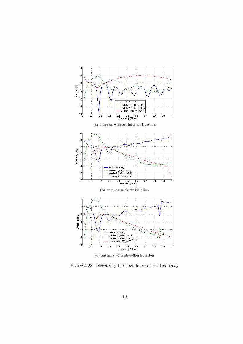
(a) antenna without internal isolation
(b) antenna with air isolation
(c) antenna with air-teflon isolation
Figure 4.28: Directivity in dependance of the frequency
49

4.3 Folded Bow-tie Antenna: Second shape
The second candidate is also a folded bow-tie loop antenna. However, now the angleα is not chosen on the top, it is chosen on the side, as Figure 4.29 shows. This is themain difference from the first candidate.
(a) Perspective view (b) Top wiew
Figure 4.29: Second candidate: original antenna dimensions
The feeding gap has been isolated since the beginning, and the best distance is1mm. Nevertheless, the best dimensions for the isolated region will have to be checked,because it changes the behavior of the return loss in some frequencies.
Figure 4.30: S11 of original second candidate
The results of the FEKO’s simulation for this original shape indicate:
1. The return loss is less than -10dB from 110MHz (Figure 4.30).
50
2. The behavior is UWB because the bandwidth is greater than 500MHz (Figure4.30). However, there is a peak at 620MHz that does not let to reach a largerbandwidth. With the parameters optimization it is expected to remove this peak.
4.3.1 Parametric study
The parametric study of the second candidate is presented, where the parameters toanalyze are:
• Angle (α)
• Thickness (T)
• Feeding region
The original parameters are shown in Figure 4.29. These original values have beentaken because they are similar of the typical bow-tie and loop parameters. The mostsuitable antenna will be found changing these values and comparing them to the originalones. The size is not taken into account because, as it has been checked in the study ofthe first candidate, the variation of the radius only changes the frequency range wherethe antenna is matched. Thus, the size of the shape will depend on the applicationrequirements.
Angle
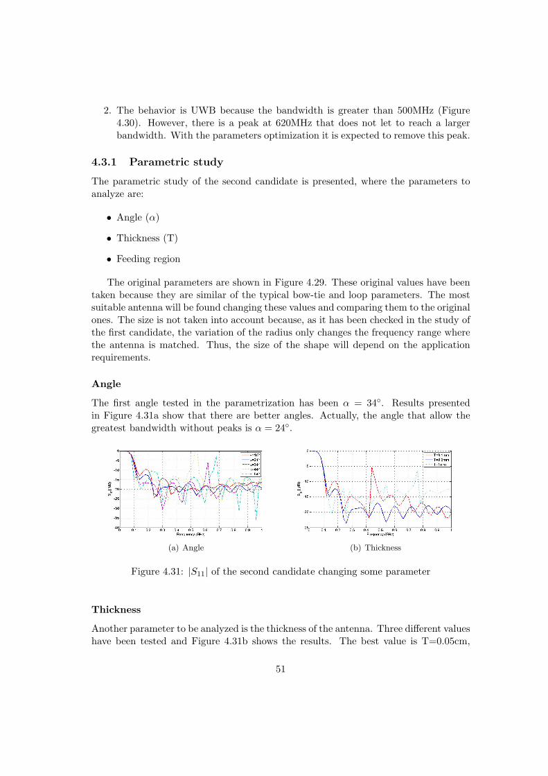
The first angle tested in the parametrization has been α = 34. Results presentedin Figure 4.31a show that there are better angles. Actually, the angle that allow thegreatest bandwidth without peaks is α = 24.
(a) Angle (b) Thickness
Figure 4.31: |S11| of the second candidate changing some parameter
Thickness
Another parameter to be analyzed is the thickness of the antenna. Three different valueshave been tested and Figure 4.31b shows the results. The best value is T=0.05cm,
51

because the return loss does not have peaks above -10dB. The other values have abehavior with a lot of irregularities and peaks.
Feeding region
The feeding split is 1mm because the region is isolated from the water, as it has beenseen in last sections. Nevertheless, the dimensions of the isolated region where thefeeding is placed can be modified to improve the return loss level (Table 4.3).
Table 4.3: Tested dimensions (in cm) of the air region to isolate the feedingCase Width (FW) Depth (FD) Height (FH)
Original one 0.1 0.2 0.15First case 0.2 0.4 0.2
Second case 0.4 0.8 0.3Third case 0.8 1.6 0.4
(a) Studied parameters of the iso-lated region
(b) S11 of the different sizes of the isolated region (α = 24)
Figure 4.32: Isolated region of the second candidate
Figure 4.32b shows the results of the four sizes tested for the antenna with an angleα = 24. It can be observed that the best options are the first case or the second case.In next sections both cases will be studied with internal isolation.
Final dimensions
The result of the parametrization of this antenna is a folded bow-tie antenna with thedimensions shown in the Figure 4.33. Notice that the feeding region has two options,the first and the second case studied in last section.
The return loss is shown in Figure 4.34, and the radiation pattern in Figure 4.35(the radiation pattern of both cases is almost the same).
The results of the FEKO’s simulation indicate:
52

(a) feeding region (b) profile view
Figure 4.33: Dimensions of the final antenna
Figure 4.34: S11 of the new antenna and the old one
1. In both cases the return loss is less than -10dB from 110MHz (Figure 4.34), thesame frequency as the original one.
2. The peak at 620MHz with a level above -10dB has been removed. Actually, inthe second case any peak in this frequency cannot be found, while in the firstcase there is a peak below -10dB.
3. The behavior is UWB because the bandwidth is greater than 500MHz, it is from110MHz to more than 1GHz.
4. In Figure 4.35 indicates that the radiation pattern is almost omnidirectional,specially in the frequencies close to 150MHz. However, in higher frequencies, it
53

(a) 151MHz (b) 292MHz
(c) 454MHz (d) 596MHz
Figure 4.35: Radiation pattern of the second candidate without internal isolation
is not totally omnidirectional because when the length of the ring is greater thana half-wave dipole, some new nulls and some new lobes in the pattern appear.
4.3.2 Final shape with internal isolation
The isolation of the antenna’s center has been done at the same way as the first can-didate (Figure 4.36).
(a) air ball (b) air-teflon ball
Figure 4.36: Second candidate with internal isolation
54

The solution consists of placing an air sphere or an air-teflon (teflon has an εr of2.1) sphere in the middle of the final shape with the improved dimensions. The changesin the behavior of the two final cases of this antenna will be studied.
Return loss
Figure 4.37 shows the |S11| results of the three models proposed of the second antennacandidate: the antenna without internal isolation, with an air ball, and with an air-teflon ball. Two sizes of the feeding region are tested:
(a) 1st case of feeding region dimensions
(b) 2nd case of feeding region dimensions
Figure 4.37: S11 of the two cases of the second candidate with and without internalisolation
• In the first case, the first thing that can be noticed is that the return loss level
55

starts to be lower than -10dB in the same frequency (110MHz) in the threeantennas (with and without internal isolation). However, when there is internalisolation, there are some frequencies with a level higher than -10dB, specially inthe case of the air-teflon sphere. This bad behavior is due to the effect of theisolated region in the feeding. If some parameters of the rectangular region wherethe feeding is placed are changed better results can be obtained.
• In the second case, it can be seen that the return loss level does not have anypeak above -10dB in the three curves. It can also be observed that when anair-teflon ball is placed as internal isolation, the |S11| level starts to be less than-10dB before than the other cases, at 90MHz. This is a good result because, asfar as we know, the propagation of electromagnetic waves in water is better withthe lowest possible frequencies.
Therefore, it can be concluded that the best shape in this antenna’s candidate is thesecond case of the feeding region (Figure 4.37b) where the dimensions were shown inFigure 4.33a (FW=0.4cm, FD=08cm, FH=0.3cm). The three models are UWB with abandwidth greater than 900MHz, but with the internal isolation the return loss level isclose to -10dB. However, it is not a problem while it was lower than this value becauseit means that more than the 90% of the power is transmitted.
Radiation Pattern
The best dimensions for the second antenna candidate have already been chosen andthe return loss level of it has been analyzed. Now it is also important to study the 3Dradiation pattern in some frequencies to check if it is omnidirectional or not.
(a) without internalisolation
(b) with air isolation (c) with air-teflon iso-lation
Figure 4.38: 3D radiation pattern at 191MHz
As Figure 4.38,4.39 and 4.40 show, the behavior of the radiation pattern in eachcase is totally different:
• At low frequencies (over to 200MHz) the radiation pattern of the three modelsare almost the same. The pattern is omnidirectional in the XY plane. In themodel without internal isolation it is possible to observe that a secondary lobe
56

(a) without internalisolation
(b) with air isolation (c) with air-teflon iso-lation
Figure 4.39: 3D radiation pattern at 393MHz
appears in the top of the shape. In the other patterns that does not occurbecause the permittivity in the center of the antenna is different, and it changesthe wavelength of the radiate waves. The lobes appear when the length of thering of the antenna is greater than a half-wave dipole.
• At medium frequencies (over to 400MHz) the pattern is different in each case. Inthe first model, the intensity of the signal is transmitted mostly in the bottomof the shape. In the second one, the transmission is done mostly in the bottomand in the middle. Finally, in the third case, the antenna radiates mostly of thepower in the middle of the antenna (XY plane). In addition, when the antennahas internal isolation, the pattern is more omnidirectional because there are lesslobes due to the smaller length of the wavelengths.
(a) without internalisolation
(b) with air isolation (c) with air-teflon iso-lation
Figure 4.40: 3D radiation pattern at 596MHz
• At high frequencies (over 600MHz) the first model is very different of the othermodels. It radiates mostly of the energy in the bottom while, when there isinternal isolation, the main lobes are in the middle and in the top of the an-tenna. In addition, when the antenna has internal isolation, the pattern is moreomnidirectional because there are less lobes than the first model.
It can be also analyzed the radiation pattern in two dimensions in XZ plane (Figure4.41) to study the behavior of the radiation pattern from another point of view.
57
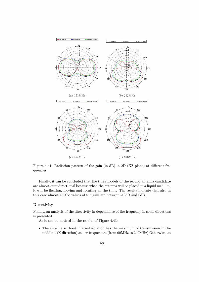
(a) 151MHz (b) 292MHz
(c) 454MHz (d) 596MHz
Figure 4.41: Radiation pattern of the gain (in dB) in 2D (XZ plane) at different fre-quencies
Finally, it can be concluded that the three models of the second antenna candidateare almost omnidirectional because when the antenna will be placed in a liquid medium,it will be floating, moving and rotating all the time. The results indicate that also inthis case almost all the values of the gain are between -10dB and 0dB.
Directivity
Finally, an analysis of the directivity in dependance of the frequency in some directionsis presented.
As it can be noticed in the results of Figure 4.43:
• The antenna without internal isolation has the maximum of transmission in themiddle 1 (X direction) at low frequencies (from 90MHz to 240MHz) Otherwise, at
58

Figure 4.42: Spherical coordinates and points of interest
frequencies from 240MHz the mostly part of the energy is radiated in the bottom.The radiation in the middle 2 (Y direction) and in the top (Z direction) is notreally good because the directivity oscillates in dependance of the frequency.
• In the cases of air and an air-teflon isolation, the radiation is higher in the middle1 at low frequencies (from 90MHz to 250MHz in the model with air, and from90MHz to 220MHz in the model with air-teflon). In the next 100-150MHz thedirection with more radiation intensity is the bottom (-Z direction), and finallyfrom 380Mhz the middle 2 (Y direction) has the higher directivity. In these caseswith internal isolation, the top of the antenna (Z direction) and the middle 2(Y direction) have also a curve with some oscillations, but not as sharp as theantenna without isolation. Notice that in high frequencies (from 500MHz) thedirectivity in the middle 1 (X direction) is very low, about -10dB.
It is also interesting to realize that almost all the level of the directivity is between-10dB and 5dB. If the radiation pattern was totally omnidirectional, the directivitywould be 0dB in all the directions (like a perfect sphere). Otherwise, if the radiationpattern was directional, the directivity would be more than 0dB in some directions andless than 0dB in the rest of the pattern. Hence it can be concluded that the directivityof this antenna is different in each case and in each direction. Nevertheless, because ofthe continuous movement of the device where the antenna will be placed, the behavioris quite correct.
59

(a) antenna without internal isolation
(b) antenna with air isolation
(c) antenna with air-teflon isolation
Figure 4.43: Directivity in dependance of the frequency
60

4.4 Folded Bow-tie Antenna: Third shape
Finally, the shape of the third candidate is presented. It is also a folded bow-tie loopantenna with the angle chosen on the side (as Figure 4.44b shows), but now the antennais not a loop. This is the main difference from the second candidate.
In the beginning of the design of this new candidate, the same dimensions that thesecond antenna candidate have been chosen, but cutting the bottom of it.
(a) Perspective view (b) Top wiew
Figure 4.44: Third candidate: original antenna dimensions
The feeding gap has been isolated since the beginning, and the best distance is1mm. Nevertheless, the best dimensions for the isolated region will have to be checked,because it changes the behavior of the return loss in some frequencies.
The results of the FEKO’s simulation for this original shape indicate:
1. The return loss is less than -10dB from 380MHz (Figure 41) because there is apeak between 300MHz and 400MHz above -10dB. If it was possible to removeit with the parametrization, the return loss would be less than -10dB from over200MHz.
2. The behavior is UWB because the bandwidth is greater than 500MHz (Figure4.45).
4.4.1 Parametric study
In the third antenna candidate, the parameters to improve are:
• Angle (α)
• Hight (H)
• Thickness (T)
• Feeding region
61

Figure 4.45: S11 of original third candidate
The dimensions of the original parameters are shown in Figure 4.44. These valueshave been taken because are similar of those of the second candidate. Changing themthe behavior of the antenna for the requested application will be improved. The size isnot taken into account because, as it was seen in the study of the first candidate, thevariation of the radius only changes the frequency range where the antenna is matched.Thus, the size of the shape will depend on the application requirements.
Angle
As it can be noticed in Figure 4.46, there are other angles better than α = 24. Theseones are α = 34, α = 44 and α = 54. Initially it has been taken an angle of 34 asthe best candidate to test the parametrization of the next parameters.
Figure 4.46: |S11| of the third candidate with different angles
62

Height
After finding a good angle, another parameter interesting to test is the height of theantenna (H). Figure 4.47a shows that a height of 7.5cm allows the antenna to transmitat lower frequencies.
Thickness
The thickness of the shape is also to be checked. Figure 4.47b indicates that the originalthickness of 0.05cm is the best one, because the other tested ones have a |S11| levelabove -10dB in some frequencies.
(a) Height (b) Thickness
Figure 4.47: |S11| of the third candidate changing some parameters
Feeding region
The gap of the feeding is 1mm because the region is isolated from the water and this isthe best distance. On the other hand, as it was observed in the second candidate, theregion of the feeding has an important effect on the return loss. In this section threedifferent sizes will be tested for that region apart from the original one to find the bestdimensions, as it can be noticed in Table 4.4.
Table 4.4: Tested dimensions (in cm) of the air region to isolate the feedingCase Width (FW) Depth (FD) Height (FH)
Original one 0.1 0.2 0.15First case 0.2 0.4 0.2
Second case 0.4 0.8 0.3Third case 0.8 1.6 0.4
Indeed, as it can be seen in Figure 4.48b, the first and the second candidates for thisregion of isolation are also good for our purpose. To choose the best one, the viabilityto fabricate it is to be considered. That is the reason why the second one is chosen,because it will be easier to fabricate a big air region in the feeding.
63

(a) Studied parameters of the iso-lated region
(b) S11 of the different sizes of the isolated region
Figure 4.48: Isolated region of the third candidate
Final dimensions
The result of the parametrization of this antenna is a folded bow-tie antenna with thedimensions shown in the Figure 4.49.
(a) feeding region (b) profile view
Figure 4.49: Dimensions of the final antenna
The return loss is shown in Figure 4.50, and the radiation pattern in Figure 4.51.The results of the FEKO’s simulation indicates:
1. The return loss is less than -10dB from 180MHz (Figure 4.50), a frequency lowerthan the original one.
2. The peak between 300MHz and 400MHz with a level above -10dB has been re-moved.
3. The behavior is UWB because the bandwidth is greater than 500MHz, it is from180MHz to more than 1GHz.
64

Figure 4.50: S11 of the new antenna and the old one
(a) 192MHz (b) 292MHz
(c) 454MHz (d) 596MHz
Figure 4.51: Radiation pattern of the third candidate without internal isolation
4. As it can noticed in Figure 4.51, the radiation pattern is almost omnidirectional,specially in the frequencies close to 200MHz. However, in higher frequencies, itis not totally omnidirectional because when the length of the ring is greater thana half-wave dipole, some new nulls and some new lobes appear in the pattern.
65

4.4.2 Final shape with internal isolation
As in the first two candidates, an air or air-teflon sphere is put inside the antenna toisolate the battery and the electrical circuit from the water (Figure 4.52). This isolationball implies important changes in the behavior of the antenna, hence an analysis of thesevariations is presented in this section.
(a) air ball (b) air-teflon ball
Figure 4.52: Second candidate with internal isolation
Return loss
First, we test the return loss level of the three models: without internal solation, withan air ball, and with an air-teflon ball.
(a) 1st case of feeding region dimensions
Figure 4.53: S11 of the third candidate with and without internal isolation
The results of the Figure 4.53 indicate the antenna works in a good way with theinternal air ball, but not with the internal air-teflon ball. The problem in the third
66
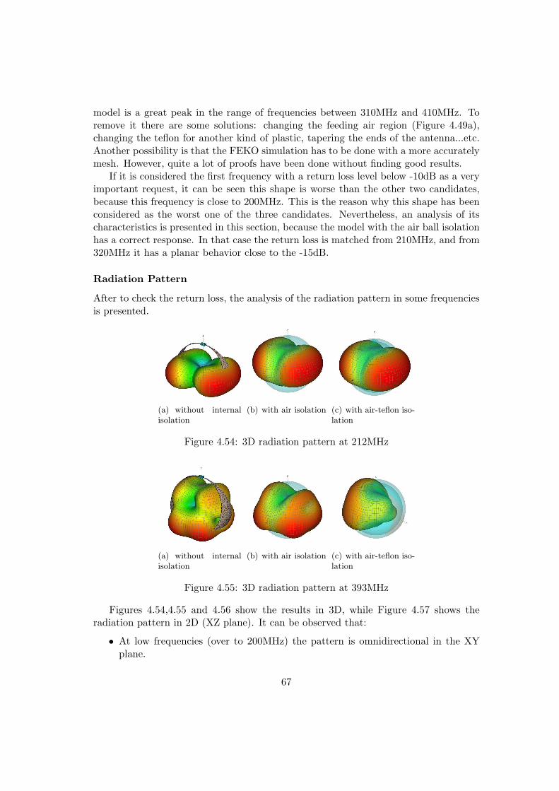
model is a great peak in the range of frequencies between 310MHz and 410MHz. Toremove it there are some solutions: changing the feeding air region (Figure 4.49a),changing the teflon for another kind of plastic, tapering the ends of the antenna...etc.Another possibility is that the FEKO simulation has to be done with a more accuratelymesh. However, quite a lot of proofs have been done without finding good results.
If it is considered the first frequency with a return loss level below -10dB as a veryimportant request, it can be seen this shape is worse than the other two candidates,because this frequency is close to 200MHz. This is the reason why this shape has beenconsidered as the worst one of the three candidates. Nevertheless, an analysis of itscharacteristics is presented in this section, because the model with the air ball isolationhas a correct response. In that case the return loss is matched from 210MHz, and from320MHz it has a planar behavior close to the -15dB.
Radiation Pattern
After to check the return loss, the analysis of the radiation pattern in some frequenciesis presented.
(a) without internalisolation
(b) with air isolation (c) with air-teflon iso-lation
Figure 4.54: 3D radiation pattern at 212MHz
(a) without internalisolation
(b) with air isolation (c) with air-teflon iso-lation
Figure 4.55: 3D radiation pattern at 393MHz
Figures 4.54,4.55 and 4.56 show the results in 3D, while Figure 4.57 shows theradiation pattern in 2D (XZ plane). It can be observed that:
• At low frequencies (over to 200MHz) the pattern is omnidirectional in the XYplane.
67

(a) without internalisolation
(b) with air isolation (c) with air-teflon iso-lation
Figure 4.56: 3D radiation pattern at 596MHz
• At medium frequencies (over to 400MHz) the radiation of the first model is mostlyin the bottom, while in the model with the air ball is almost of all in the bottomand in the middle. In the third case it is obtained a radiation pattern totallyunusual because there is not a symmetry like in the others cases. Notice thatin this frequency (393MHz) the return loss level of this third model was above-10dB.
• At high frequencies (over 600MHz) the first model has a lot of lobes, and theenergy is concentrated in the bottom of the antenna. The radiation pattern ofboth models with internal isolation are similar, and they have a behavior quiteomnidirectional, with a maximum of transmission in the middle of the sides.
The results indicate that also in this case almost of the values of the gain are between-10dB and 0dB.
Finally, it can be concluded that the the model without internal isolation and themodel with internal air isolation radiates correctly in almost all the directions. Whenthe antenna will be placed in a liquid medium, it will be floating, moving and rotatingall the time. The results indicates that also in this case almost of the values of the gainare between -10dB and 0dB.
However, the third model (air-teflon isolation) has not an omnidirectional behaviorin all the frequencies.
Directivity
The last parameter to analyze is the directivity in dependance of the frequency. InFigure 4.58 it can be observed the directions that have been studied.
In that case only the two first models have been studied (antenna without internalisolation, antenna with air inside) because the results of the third one do not have anyutility. As it can be noticed in Figure 4.59, the graphic indicates:
• The antenna without internal isolation has the maximum of transmission in themiddle 2 (Y direction) at low frequencies (from 90MHz to 240MHz) Otherwise, atfrequencies from 240MHz the mostly part of the energy is radiated in the bottom
68
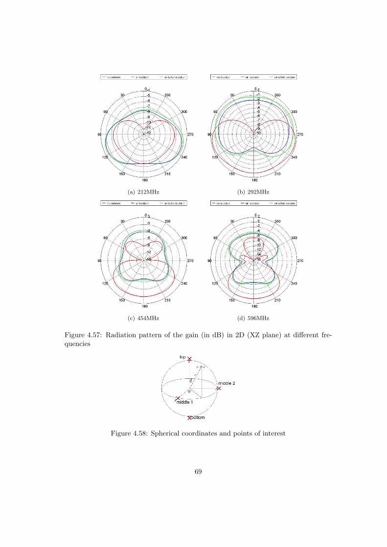
(a) 212MHz (b) 292MHz
(c) 454MHz (d) 596MHz
Figure 4.57: Radiation pattern of the gain (in dB) in 2D (XZ plane) at different fre-quencies
Figure 4.58: Spherical coordinates and points of interest
69
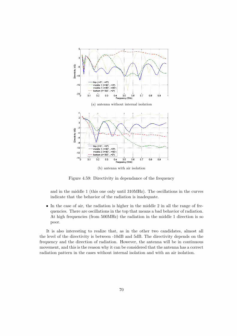
(a) antenna without internal isolation
(b) antenna with air isolation
Figure 4.59: Directivity in dependance of the frequency
and in the middle 1 (this one only until 310MHz). The oscillations in the curvesindicate that the behavior of the radiation is inadequate.
• In the case of air, the radiation is higher in the middle 2 in all the range of fre-quencies. There are oscillations in the top that means a bad behavior of radiation.At high frequencies (from 500MHz) the radiation in the middle 1 direction is sopoor.
It is also interesting to realize that, as in the other two candidates, almost allthe level of the directivity is between -10dB and 5dB. The directivity depends on thefrequency and the direction of radiation. However, the antenna will be in continuousmovement, and this is the reason why it can be considered that the antenna has a correctradiation pattern in the cases without internal isolation and with an air isolation.
70
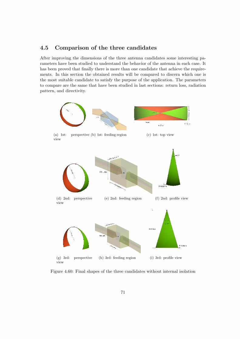
4.5 Comparison of the three candidates
After improving the dimensions of the three antenna candidates some interesting pa-rameters have been studied to understand the behavior of the antenna in each case. Ithas been proved that finally there is more than one candidate that achieve the require-ments. In this section the obtained results will be compared to discern which one isthe most suitable candidate to satisfy the purpose of the application. The parametersto compare are the same that have been studied in last sections: return loss, radiationpattern, and directivity.
(a) 1st: perspectiveview
(b) 1st: feeding region (c) 1st: top view
(d) 2nd: perspectiveview
(e) 2nd: feeding region (f) 2nd: profile view
(g) 3rd: perspectiveview
(h) 3rd: feeding region (i) 3rd: profile view
Figure 4.60: Final shapes of the three candidates without internal isolation
71

4.5.1 Final shapes
First, the three candidates without internal isolation are considered. Figure 4.60 re-minds the dimensions of each shape.
Notice that all the shapes have a radius of 5cm. However, depending on the re-quirements, the antenna could be smaller, but the first frequency with a return losslevel lower than -10dB would be higher.
Return loss
The most important parameter is the return loss. Without a good matching in thefrequency range of interest, the antenna cannot be suitable for the application.
The guidelines to choose the best antenna are:
• A return loss less than -10dB as the lowest frequency as possible, because theelectromagnetic waves in water propagate better in low frequencies.
• A large bandwidth, because the antenna has to work in a UWB network.
Following these two points, it can be concluded watching the Figure 4.61 that thebest antenna is the second one, followed by the first one. The antenna with a worstreturn loss is the third candidate.
Figure 4.61: |S11| of the three candidates without internal isolation
Radiation Pattern
The radiation pattern is also very important because an antenna as omnidirectional aspossible is preferred. The candidate which has the radiation pattern more similar to asphere will be the best one. However, it has to be taken into account that the radiationpattern changes in dependance of the frequency.
72

(a) 1st candidate (b) 2nd candidate (c) 3rd candidate
Figure 4.62: 3D radiation pattern at 200MHz
(a) 1st candidate (b) 2nd candidate (c) 3rd candidate
Figure 4.63: 3D radiation pattern at 400MHz
(a) 1st candidate (b) 2nd candidate (c) 3rd candidate
Figure 4.64: 3D radiation pattern at 600MHz
Figures 4.62, 4.63 and 4.64 show the radiation pattern of the three candidates atfrequencies close to 200MHz, 400MHz and 600MHz:
• At low frequencies (200MHz), the pattern of the second candidate is really ade-quate. The first one is also quite good, and the third one is only omnidirectionalin the XY plane.
• At medium frequencies (400MHz), the radiation pattern of the three candidatesis more or less similar referred to the omnidirectionallity.
• At high frequencies (600MHz), the third model is the most suitable to radiatein all the directions, while the first and the second radiates more in the bottomthan in the top.
73
Realizing these results, it has been also chosen the second shape as the best one inthis issue, because at low and at medium frequencies its radiation pattern is very good.
Directivity
The last parameter that is taken into account to do the selection of the best candidateis the directivity, who will tell how does the radiation intensity change in dependanceof the direction and the frequency.
As it can be noticed in Figure 4.65, the directivity of the first and the secondcandidates is almost the same, while the third one has some differences. However, thedifferences amongst them are not enough important to prioritize one candidate face upto the others.
Finally, after the comparison of these antenna candidates, it can be concluded thatthe best one is the second folded bow-tie antenna.
74

(a) 1st candidate
(b) 2nd candidate
(c) 3rd candidate
Figure 4.65: Directivity in dependance of the frequency
75

4.5.2 Final shapes with internal isolation
Now, an internal isolation has been placed inside the antenna. As it can be observedin section 4.4.2, the air-teflon internal sphere produces a bad response in the thirdcandidate. Furthermore, in the other shapes, the difference between the model withair and the model with air and teflon is not very significative. Thus, in this sectionthe cases with only air isolation will be studied. To construct it, it has been taken theoriginal shapes and it has been included the air ball inside, as in Figure 4.66.
(a) 1st candidate (b) 2nd candidate (c) 3rd candidate
Figure 4.66: Candidates with internal air isolation
Return loss
Figure 4.67 allows to realize the differences among the shapes in the return loss level. Itis possible to appreciate that the candidate with a better |S11| is the first one, becauseit starts to be lower than -10dB before the others and the level in low frequencies arelower than the others. The bandwidth of this candidate is shorter than the second andthe third candidates, but it is enough because it is bigger than 500MHz, and it meansthat is an UWB behavior.
Figure 4.67: |S11| of the three candidates with internal air isolation
76

Radiation Pattern
The internal isolation of the candidates modifies the radiation pattern. As it can bechecked in Figures 4.68,4.69 and 4.70, the first candidate is also the best, because inall the frequencies is more omnidirectional than the others.
(a) 1st candidate (b) 2nd candidate (c) 3rd candidate
Figure 4.68: 3D radiation pattern at 200MHz
(a) 1st candidate (b) 2nd candidate (c) 3rd candidate
Figure 4.69: 3D radiation pattern at 400MHz
(a) 1st candidate (b) 2nd candidate (c) 3rd candidate
Figure 4.70: 3D radiation pattern at 600MHz
Directivity
Finally, Figure 4.71 shows the directivity of each candidate in dependance of the fre-quency and in four different directions. The characteristics of these curves do notcontribute a lot to choose the best shape.
77

(a) 1st candidate
(b) 2nd candidate
(c) 3rd candidate
Figure 4.71: Directivity in dependance of the frequency
Finally, it can be concluded that when the antenna has internal isolation for thebattery and the electrical circuit, the best candidate is the first folded bow-tie antenna.
78

4.5.3 Conclusions
In this section it has been done an extensive study of the three antennas proposed foran underwater application. The dimensions have been improved till finding the bestresults in each case, and some important features of the antennas have been analyzed.After that, it has been concluded two main issues:
• The best candidate without internal isolation is the second one.
• The best candidate with internal isolation is the first one.
4.6 Variations in the medium
4.6.1 Conductivity
FEKO software provides some useful options to vary the parameters of the medium.One of these parameters is the conductivity, which has an important effect in return loss,as it has been seen in Section 2.2.1. After finding a good shape for the application inpure water (σ = 0S/m), other conductivities will be studied in the final design. Noticethat all of these simulations have been done with a constant relative permittivity of 81.
Figure 4.72: S11 of the final candidate with air-teflon isolation in different conductivities
Figure 4.72 shows the return loss of the final shape with air-teflon isolation withdifferent conductivities. As it can be seen in Section 2.2.1, the usual conductivity valuesof water (not sea water) are below 0.1S/m. Watching the graph, it can be concludedthat the level of return loss does not experiment a significative modification. Actually,the higher the conductivity is, the better the results at low frequencies are.
Conductivities higher than 0.1S/m have not been studied because, as it will beshown in next sections, the communications in water at these conductivity levels arenot possible in distances of more than half a meter.
79
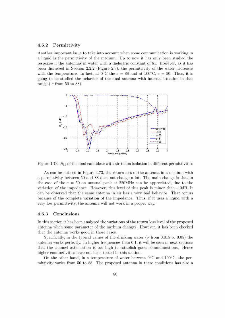
4.6.2 Permittivity
Another important issue to take into account when some communication is working ina liquid is the permittivity of the medium. Up to now it has only been studied theresponse if the antennas in water with a dielectric constant of 81. However, as it hasbeen discussed in Section 2.2.2 (Figure 2.3), the permittivity of the water decreaseswith the temperature. In fact, at 0C the ε = 88 and at 100C, ε = 50. Thus, it isgoing to be studied the behavior of the final antenna with internal isolation in thatrange ( ε from 50 to 88).
Figure 4.73: S11 of the final candidate with air-teflon isolation in different permittivities
As can be noticed in Figure 4.73, the return loss of the antenna in a medium witha permittivity between 50 and 88 does not change a lot. The main change is that inthe case of the ε = 50 an unusual peak at 220MHz can be appreciated, due to thevariation of the impedance. However, this level of this peak is minor than -10dB. Itcan be observed that the same antenna in air has a very bad behavior. That occursbecause of the complete variation of the impedance. Thus, if it uses a liquid with avery low permittivity, the antenna will not work in a proper way.
4.6.3 Conclusions
In this section it has been analyzed the variations of the return loss level of the proposedantenna when some parameter of the medium changes. However, it has been checkedthat the antenna works good in those cases.
Specifically, in the typical values of the drinking water (σ from 0.015 to 0.05) theantenna works perfectly. In higher frequencies than 0.1, it will be seen in next sectionsthat the channel attenuation is too high to establish good communications. Hencehigher conductivities have not been tested in this section.
On the other hand, in a temperature of water between 0C and 100C, the per-mittivity varies from 50 to 88. The proposed antenna in these conditions has also a
80

good return loss level. However, at low permittivities (close to air), this antenna is notuseful.
81

4.7 Transmission level and channel attenuation
Up to now it has been studied the return loss level (|S11|), but it is also importantto know the transmission level (|S21| or |S12|) between two antennas to analyze theviability of a possible network with them. In addition, there are some elements whichchange the behavior of the channel attenuation, and they have to be analyzed too, todetermine under which conditions our system will be able to work.
To do this study, it has been used a pair of dipoles with the same characteris-tics, because the folded bow-tie antenna requests too much computational resources toperform this study. Some FEKO simulations have been done, changing the distancebetween the dipoles and changing also the conductivity of the medium to compare theresults.
4.7.1 Dipoles in air
First of all, we analyze the transmission level of the pair of dipoles in air to be able tocheck the differences in water. We have tried a 300MHz frequency because it is one ofthe most representative frequencies inside the bandwidth of the application.
In that case, the dipoles have a length of 0.5 meters (λ = 1m). If we take a lookto an old Section (2.2.5), we can see that the work frequency is 300MHz (2.10). The|S21| has been studied between the two dipoles in a range of frequencies from 10MHzto 500MHz, and a distance from 10 centimeters to 3 meters.
As you can observe in Figure 4.74, the attenuation changes depending on the dis-tance and on the frequency. The maximum transmission level is always around thework frequency of 300MHz, but the level in that frequency decreases with the distance.
Figure 4.74: Transmission level between two dipoles in air, in different distances (inmeters)
However, Figure 4.74 does not give a perfect idea about the effect of the distance in
82

Figure 4.75: Transmission level between two dipoles in air at work frequency (300MHz),in different distances (in meters)
the attenuation. Otherwise, Figure 4.75 shows the transmission level between the pairof dipoles always at the same frequency (300MHz) but changing the distance. In thatcase it is easier to understand the behavior of the level’s decrease. In a few centimetersof distance, the effect of the distance’s increment in the transmission level is greaterthan in a longer distances.
4.7.2 Dipoles in water
As far as we know, the dimensions of the antennas in water can be 9 or 10 times smallerthan in air with the same results. The reason for this is that we have taken a pair ofdipoles of 6cm of length (λ = 1/9 = 0.11m) to study the transmission level in waterand be able to compare the results.
The range of frequency taken into account for this simulation is the same one asthe range in the last section (from 10MHz to 500MHz). We have chosen this rangeof frequencies because it is similar than the range of the interest for the underwaterapplication that we are studying. The distances studied are also the same as the lastsection: from 10 centimeters to 3 meters.
In Section (2.2.1) the conductivity was presented of different kinds of water. Astudy of the transmission level of these different waters is presented.
Dipoles in pure water (σ ≈ 0)
The two dipoles are placed now in an almost ultra pure underwater background, witha permittivity of 81 and a null conductivity.
From Figure 4.76 you can observe the behavior of the |S12| in water without con-ductivity. It depends of the frequency and the distance, and as we can see, the graphic
83

is different as the previous one in air. The main difference is that in water the trans-mission is not as narrow-band as in air.
Figure 4.76: Transmission level between two dipoles in pure water, in different distances(in meters)
Figure 4.77: Transmission level between two dipoles at work frequency, in differentdistances (in meters)
Figure 4.77 shows that the difference of the transmission level in dependance of thedistance between the air and the pure water is almost always 5dB. However, the trendof the curve is the same in both cases.
Dipoles in water with conductivity (σ > 0)
Now, an analysis of the transmission level in impure waters is presented. In Figure 4.78and Figure 4.79 it can be checked that the |S12| decreases with the conductivity level.
84
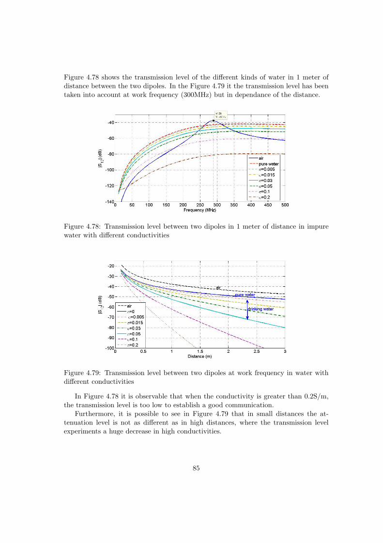
Figure 4.78 shows the transmission level of the different kinds of water in 1 meter ofdistance between the two dipoles. In the Figure 4.79 it the transmission level has beentaken into account at work frequency (300MHz) but in dependance of the distance.
Figure 4.78: Transmission level between two dipoles in 1 meter of distance in impurewater with different conductivities
Figure 4.79: Transmission level between two dipoles at work frequency in water withdifferent conductivities
In Figure 4.78 it is observable that when the conductivity is greater than 0.2S/m,the transmission level is too low to establish a good communication.
Furthermore, it is possible to see in Figure 4.79 that in small distances the at-tenuation level is not as different as in high distances, where the transmission levelexperiments a huge decrease in high conductivities.
85

4.7.3 Conclusions
In this section it has been studied the transmission level between two dipoles in differentmediums (air, pure water, impure water).
It has been concluded that in water the attenuation is greater, specially in waterswith an impurity superior than common drinking waters (0.05S/m). Moreover, thedistance is very important to determinate if the communication between two antennasis suitable or not. Thus, there are two important factors to take into account in anunderwater transmission: the conductivity of the medium and the distance betweenthe antennas.
86

Chapter 5
Conclusions and future work
In this thesis an antenna for UWB underwater applications has been designed. Inorder to understand the goal of the thesis, first it has been given an overview of thecharacteristics of UWB technology, underwater propagation and classes of suitableantennas for our application. Two software tools have been analyzed to find out whichone is the most suitable for underwater applications. Some antennas have been analyzedwith FEKO software to find a shape for our application. The behavior of two of theseantennas (loop and bow-tie) in water has proven to be a good beginning to the design.A combination of these shapes has resulted in a new antenna shape: the folded bow-tieantenna. An analysis of three candidates of this new antenna has been presented. Inaddition, the isolation problem of the feeding antenna from the water has been takeninto account in the design, adding also an internal isolation to be able to isolate thebattery and the electrical circuit from the water. Next, a full comparison has beendone to choose the best shape to achieve the requirements of the application. Afterfinding the best antenna, some variations of the water properties have been done inorder to study the effect of them in the behavior of the antenna. Finally, a study of thetransmission level and channel attenuation in water (pure and impure) is presented.
The main conclusions are:
• FEKO software is the most suitable software for the UWB antenna design forunderwater communications, mainly due to the mesh simulation properties andalso due to the computational environment properties flexibility.
• The circular loop antenna and the bow-tie shapes are good starting points forthe design. The return loss of the combination of both shapes in water shows apromising behavior.
• Three candidates have been found as a good shapes.
• The second candidate is the best one without internal isolation.
• If an internal isolation is placed inside the antenna, the best candidate is the firstone.
87
• The third candidate does not show a good behavior when an isolation of air andteflon is placed inside.
• The size of the antenna is an important factor to take into account. The biggerthe size is, the better the return loss level in low frequencies is.
• The changes in the medium of propagation affect at the return loss level of theantenna. However, the typical values of the conductivity and the permittivity ofwater do not affect this parameter too much.
• The transmission level in pure water is 5dB lower than in air. However, if the con-ductivity increases, the channel attenuation increases too. Conductivities greaterthan σ=0.1S/m do not allow a good communication in devices with more than50cm of separation.
Future work includes manufacturing the antenna for the Smart-PEAS project de-veloped at CAS. Then rigorous measurements of the antenna in the laboratory wouldbe necessary to compare the results obtained with the simulations done in this thesis.It will allow proving the viability of the antenna in the project.
88
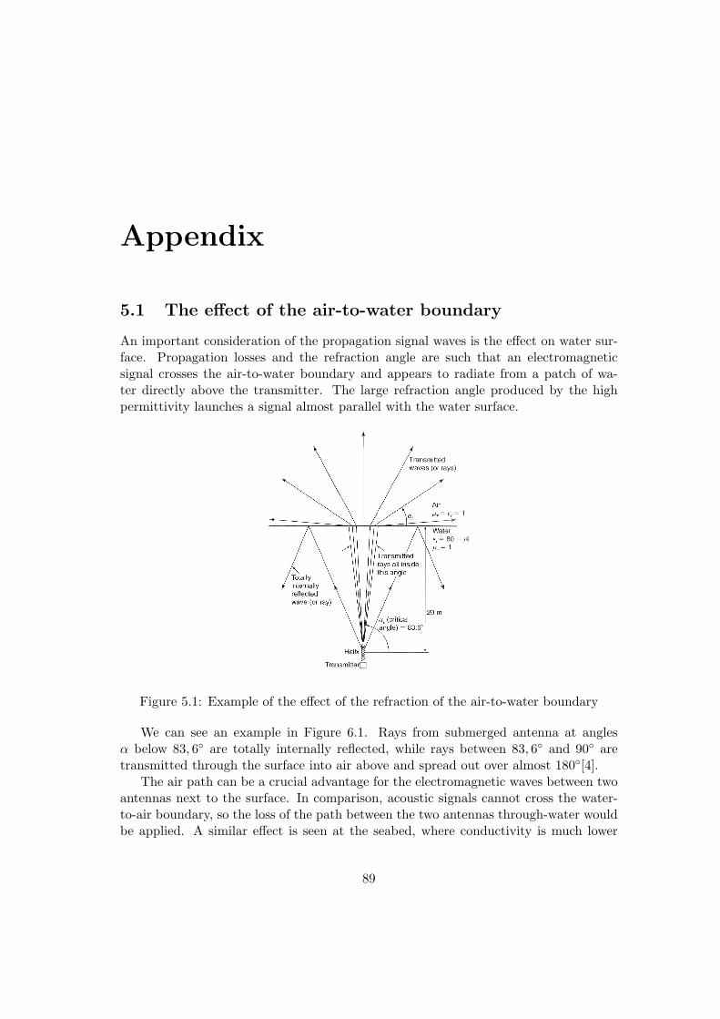
Appendix
5.1 The effect of the air-to-water boundary
An important consideration of the propagation signal waves is the effect on water sur-face. Propagation losses and the refraction angle are such that an electromagneticsignal crosses the air-to-water boundary and appears to radiate from a patch of wa-ter directly above the transmitter. The large refraction angle produced by the highpermittivity launches a signal almost parallel with the water surface.
Figure 5.1: Example of the effect of the refraction of the air-to-water boundary
We can see an example in Figure 6.1. Rays from submerged antenna at anglesα below 83, 6 are totally internally reflected, while rays between 83, 6 and 90 aretransmitted through the surface into air above and spread out over almost 180[4].
The air path can be a crucial advantage for the electromagnetic waves between twoantennas next to the surface. In comparison, acoustic signals cannot cross the water-to-air boundary, so the loss of the path between the two antennas through-water wouldbe applied. A similar effect is seen at the seabed, where conductivity is much lower
89

than in the water.The refraction loss due to the change in the medium can be defined on (6.1) [4]:
γRL= −20 log 7.4586× 10⁻⁶ ×
√f/σ (5.1)
where γRLis the refraction loss in dB.
This effect of the channel is important in the Smart-PEAS project because the paththrough the air may be better than for water, but the analysis of this effect is not ourgoal.
90
References
1. Marc Rhodes, ”Underwater Electromagnetic Propagation”, http://www.hydro-international.com/issues/articles/ id697-Underwater ElectromagneticPropagation.html
2. Alle-Jan van der Veen and Geert Leus, ”Signal processing for communications”,Delft University of Technology
3. Ahmed I. Al-Shammaa, Andrew Shaw, and Saher Saman, ”Propagation of Elec-tromagnetic Waves at MHz Frequencies Through Seawater”, IEEE Transactionson antennas and propagation, Vol. 52, No. 11, November 2004
4. Lloyd Butler, ”Underwater Radio Communication”, http://www.qsl.net/ vk5br/UwaterComms.htm
5. Hansen, R C., ”Radiation and Reception with Buried and Submerged Antennas”,IEEE Transactions on Antennas and Propagation, May 1963.
6. ”Linear and loop antennas”, www.ece.rutgers.edu/ orfanidi/ewa/ch16.pdf
7. Daniel Andersson, ”Design Challenges for UWB radar design”, radarbolaget, 2008
8. Alexander Vorobyov, ”Planar Elliptically Shaped Dipole Antenna Radio”, pp.1-7, 2008
9. ”First Report and Order (FCC 02-48). Action by the Comission February 14,2002. New Public Safety Applications and Broadband internet access amonguses envisioned by FCC authorization of Ultra-Wideband Technology”.
10. Balanis, ”Antenna Theory, Analysis and Design”.
11. CST MICROWAVE STUDIO, Tutorials, CST-Computer Simulation Technology,2003.
12. K. Kurokawa, ”Power waves and the scattering matrix”, Microwave Theory andTechniques, IEEE Transactions on, vol. 13, no. 2, pp. 194-202, Mar 1965.
13. ”IEEE standard definitions of the terms for antennas”, IEEE Transactions onAntennas and Propagations, vol. AP-31, no. 6, 1983.
91

14. M. Pausini, ”Autocorrelation Receivers for Ultra Wideband Wireless Communi-cations”, pp 10-12, 2007.
15. ”Kaye & Laby, Tables of Physical and Chemical Constants, National PhysicalLaboratory, http://www.kayelaby.npl.co.uk/
16. Vyacheslav V. Komarov and Juming Tang, ”Dielectric Permittivity and loss fac-tor of tap water at 915MHz”, MICROWAVE AND OPTICAL TECHNOLOGYLETTERS Vol. 42, No. 5, September 2004
17. Schlumberger Excellence in Educational Development, ”Conductivity of water”,http://www.seed.slb.com
18. Martin Chaplin, ”Water structure and science”, http://www.lsbu.ac.uk/water/microwave.html
92