vacuum polarization solver - ulisboa · a special thanks to some of my best, most inspirational...
TRANSCRIPT

Vacuum Polarization SolverPedro Vidal Cabrita Carneiro
Thesis to obtain the Master of Science Degree in
Engineering Physics
SupervisorsProf. Luís Miguel de Oliveira e Silva
Dr. Thomas Emmanuel Aurelien Grismayer
Examination CommitteeChairperson: Prof.Luís Paulo da Mota Capitão Lemos Alves
Supervisor: Dr. Thomas Emmanuel Aurelien GrismayerMembers of the Committee: Prof. Vasco António Dinis Leitão Guerra
Prof. José Tito da Luz Mendonça
September 2016


iii
AcknowledgementsThe thesis about to be presented, which I am very proud of, is the result of thousands of hours in-
vested by many people both directly in the work, but also invested in my development by the meansof education and/or friendship. I will attempt to do justice by thanking all of you.
To Thomas Grismayer, one of my supervisors and the older brother I never had; thank you for allthe amusing hours we spent together producing this work, but also for all the physics you taughtme and for all the fun we had researching things like how many times Sommerfeld was nominatedfor Nobel prize, how many red cards Sergio Ramos has had. Besides being an excellent supervisor,you taught me valuable personal skills to overcome my shyness and always leading our work bygiving the example of never giving up and placing the quality of the physics above all else. To myother supervisor, Luís Oliveira e Silva, for all you invested in me, for your availability to solve everyproblem in order to protect your own, your strategic vision regarding the frontiers of science and forworking in your sleep to provide outstanding conditions to all researchers at the Group of lasers andPlasmas (GoLP). One thing we all learned for sure is that there are certain carriages in German trainsin which one must be careful when talking!
To my teachers in MEFT, I believe you never get enough credit for your work (just the opposite infact). A special thanks to some of my best, most inspirational teachers, Vasco Guerra, Filipe Joaquim,Luís Lemos Alves, Nuno Loureiro, Jorge Romão and Teresa Peña.
To Isabel Ribeiro, a true mentor since day 1, to whom I owe so much.
To my friends, Rui André present from the moment we changed course to physics, always readyto put the well-being of others above your own and to play ’cabecudos’, André Martins for proof-reading my thesis and for our friendship that will surely last, Fábio Cruz for your true friendshipand for our great travels (uhh, laser, yes yes), Paulo Ratinho for all the fun conversations but also forwhat you taught me and your honest advice, and Vitor Hariton for our afternoon conversations. Tomy Squadra Azzura, specially Fabrizio, for our deep conversations and sincere friendship. To SwenKünzel, for always knowing what the status is and mentoring me through these years by teachingme to challenge common thought.To all the people at GoLP for all the pleasent lunches, team meetings and GoLP days. Thank youto Nitin since day one, Marija for her constant energy, Jorge for our pleasent conversations, Ricardofor all his help on the tricky technical aspects but also for always being available and all other teammembers for the great time we all had.
To my Family, you deserve a special acknowledgment. To my father and brother for being my bestfriends; I will always treasure all the benfica games, golf matches and so many other great moments.To my sister, please remain confident and true. To all my cousins for always looking up to me andsupporting me. Finally, to my grandparents, who always tooke me in as their son and moulded mycharacter. To my grandmother, Maria do Carmo, you took me in 6 years ago and took care of me as a

iv
true son. I am glad to have become your friend and come to admire you’re attitude towards others.To my mother for all her love, sacrifice and hard work to assure me and my brothers had the besteducation and conditions to thrive in happiness, I would like to dedicate this work to you :)
To Marta, for all her sacrifice during the past 5 years so that I could achieve my academic and pro-fessional goals; for all the voltinhas that kept me mentally sane and all the programs at Azambuja,Algarve, Poland, London... you name it. Essentialy, thank you for loving me and making me happy.

v
ResumoNeste trabalho, abordamos a dinâmica do vácuo quântico usando uma teoria semi-clássica desen-volvida por Heisenberg-Euler que trata o vácuo como um meio effetivo introduzindo uma polar-ização e magnetização, não lineares, como correções às equações de Maxwell. Começamos porrever a origem e validade da teoria desenvolvida efetuando ainda uma revisão da literatura teórica,numérica e experimental. De seguida, apresentamos o resultado do principal objetivo do trabalho: odesenvolvimento de um novo método numérico para resolver o conjunto de equações de Maxwell-Heisenberg-Euler, pela primeira vez, em multi-dimensões.
Testamos a precisão do algoritmo desenvolvido, reproduzindo em 1D a birrefringência do vácuoe a geração de harmónicas num cenário em que se contra-propagam duas ondas planas. A versatil-idade do código é demonstrada em 2D ao apresentar resultados de simulações de interações entre2 impulsos Gaussianos, com parâmetros realistas, que permitem a geração de harmónicas mais ele-vadas.
Finalmente, fazemos uma análise das assinaturas experimentais que podemos esperar em cenáriosrealistas. Para tal, consideramos um cenário em que se faz interagir um laser ultra-intenso de fre-quência ótica, com um laser raio-X a sondar o vácuo quântico. Demonstramos a existência de umaelliticidade induzida na polarização da sonda raio-X, tal como uma rotacão no ângulo de polarização.Estes resultados finais mostram a utilidade da ferramenta numérica desenvolvida neste trabalho, talcomo as respectivas análises teóricas, que complementam todo o trabalho teórico e experimental de-senvolvido pela comunidade, com o objetivo de detetar o vácuo quântico.
Palavras Chave: Vácuo Quântico, Heisenberg-Euler, Algoritmo numérico, Equações de Maxwell


vii
AbstractIn this work we address the quantum dynamics of the vacuum using a semi-classical theory
developed by Heisenberg-Euler, treating the vacuum as an effective nonlinear medium by correctingthe classical Maxwell’s equations with a polarisation and magnetisation of the vacuum. We beginwith a review of the derivation and validity of the theory and perform a review of the theoretical,numerical and experimental literature on the subject.
We present the result of the main objective of this thesis: the development of a new numer-ical method to solve the set o Maxwell-Heisenberg-Euler equations, for the first time, in multi-dimensions.
We then test the precision of the algorithm by reproducing in 1D the birefringence of the vacuumand by comparing the generation of high harmonics in the counter-propagation of two plane waves.The robustness of the code is demonstrated in 2D with simulations of the interaction between twoGaussian pulses, with realistic parameters, generating the respective high harmonics.
Finally, we perform a theoretical analysis and corresponding simulations, of the experimentalsignatures that can be expected in realistic scenarios. We consider an X-ray laser pulse probing thequantum vacuum by interacting with an ultra-intense optical laser pump. Our results show that anellipticity is induced in the polarisation of the probe laser, but also a rotation in the angle of polar-isation. These results show the usefulness of the numerical tool developed in this work, and therespective theoretical analysis, thus complementing the community’s current theoretical and experi-mental effort to detect the quantum vacuum.
Key words: Quantum Vacuum, Heisenberg-Euler, Numerical algorithm, Maxwell’s Equations


ix
Contents
Acknowledgements iii
Resumo v
Abstract vii
1 Introduction 11.1 Vacuum . . . . . . . . . . . . . . . . . . . . . . . . . . . . . . . . . . . . . . . . . . . . . . 11.2 Motivation . . . . . . . . . . . . . . . . . . . . . . . . . . . . . . . . . . . . . . . . . . . . 21.3 Theoretical framework . . . . . . . . . . . . . . . . . . . . . . . . . . . . . . . . . . . . . 31.4 PIC method . . . . . . . . . . . . . . . . . . . . . . . . . . . . . . . . . . . . . . . . . . . 51.5 State of the Art . . . . . . . . . . . . . . . . . . . . . . . . . . . . . . . . . . . . . . . . . . 6
2 Numerical methods: QED solver 92.1 Maxwell equation solver: Yee Scheme . . . . . . . . . . . . . . . . . . . . . . . . . . . . 9
2.1.1 Summary . . . . . . . . . . . . . . . . . . . . . . . . . . . . . . . . . . . . . . . . 92.1.2 Numerical discretisation of Maxwell equations . . . . . . . . . . . . . . . . . . . 10
2.2 QED solver: generalized Yee scheme . . . . . . . . . . . . . . . . . . . . . . . . . . . . . 122.2.1 Interpolation of the fields . . . . . . . . . . . . . . . . . . . . . . . . . . . . . . . 14
2.3 Algorithm Stability: linear and nonlinear analysis . . . . . . . . . . . . . . . . . . . . . 152.4 Osiris implementation . . . . . . . . . . . . . . . . . . . . . . . . . . . . . . . . . . . . . 21
2.4.1 Code inputs . . . . . . . . . . . . . . . . . . . . . . . . . . . . . . . . . . . . . . . 212.4.2 Structure of solver . . . . . . . . . . . . . . . . . . . . . . . . . . . . . . . . . . . 212.4.3 Diagnostics developed . . . . . . . . . . . . . . . . . . . . . . . . . . . . . . . . . 22
3 Simulation results and code benchmarks 253.1 1D Results . . . . . . . . . . . . . . . . . . . . . . . . . . . . . . . . . . . . . . . . . . . . 25
3.1.1 Vacuum Birefringence . . . . . . . . . . . . . . . . . . . . . . . . . . . . . . . . . 263.1.2 Counter-propagating plane waves . . . . . . . . . . . . . . . . . . . . . . . . . . 293.1.3 1D Birefringence revisited: Green function formalism . . . . . . . . . . . . . . . 32
3.2 2D Results . . . . . . . . . . . . . . . . . . . . . . . . . . . . . . . . . . . . . . . . . . . . 343.2.1 2D vacuum birefringence . . . . . . . . . . . . . . . . . . . . . . . . . . . . . . . 343.2.2 Counter-propagation of Gaussian laser pulses . . . . . . . . . . . . . . . . . . . 35
4 Realistic scenarios of vacuum birefringence 414.1 Setup and theoretical framework . . . . . . . . . . . . . . . . . . . . . . . . . . . . . . . 41
4.1.1 Vacuum Birefringence: probing the quantum vacuum . . . . . . . . . . . . . . . 41

x
4.1.2 Birefringence in a static field revisited . . . . . . . . . . . . . . . . . . . . . . . . 424.1.3 Post-processing diagnostic: polarization diagnostic . . . . . . . . . . . . . . . . 44
4.2 2D Birefringence with a realistic pump profile . . . . . . . . . . . . . . . . . . . . . . . 484.2.1 Solving the wave equation using the WKB approximation . . . . . . . . . . . . 504.2.2 Derivation of the dispersion relation . . . . . . . . . . . . . . . . . . . . . . . . . 514.2.3 Simulation result analysis . . . . . . . . . . . . . . . . . . . . . . . . . . . . . . . 54
5 Conclusions and future prospects 61
Bibliography 65
A Appendix 71

xi
List of Figures
1.1 The fundamental QED vertex. This vertex is deduced from the QED Lagrangian den-sity when a coupling between a relativistic fermion and a EM field is included. Thecoupling constant is the electron charge e. Using combinations of the fundamentalvertex, all interactions and processes in QED can be represented. . . . . . . . . . . . . 3
1.2 Feynman diagram of light-by-light scattering. This is the interaction that triggers thevirtual vacuum polarization. The naming of "virtual" polarization is due to the factthat the electron-positron pairs are generated as internal fermionic lines in the diagram 3
1.3 Matterless double slit setup: lenses L1 and L2, focus two ulta-intense gaussian pulsesare counterpropagated at a small and symmetric angle to a probe pulse with a muchlarger waist leading to an interference pattern in the screen S (b). Figure 1 in originalarticle [32] . . . . . . . . . . . . . . . . . . . . . . . . . . . . . . . . . . . . . . . . . . . . 8
2.1 One dimensional spatial grid illustrating the disposition of the electric and magneticfields. This illustrates the fact that the both fields are staggered both in space and in time 11
2.2 Full loop of the modified Yee scheme . . . . . . . . . . . . . . . . . . . . . . . . . . . . . 132.3 Two-dimensional Yee grid cell . . . . . . . . . . . . . . . . . . . . . . . . . . . . . . . . . 152.4 Amplitude of EM invariantE2−B2 as a function of the seeded k-mode for a resolution
∆x = π/100, ∆t = 0.98∆x and ξE20 = 10−4. Simulation results in blue are compared
to eq.2.16 in red. . . . . . . . . . . . . . . . . . . . . . . . . . . . . . . . . . . . . . . . . . 172.5 Imaginary part of solution of nonlinear dispersion relation, eq.(2.12), as a function of
k-mode, calculated using three different methods. Simulation parameters used were∆x = 0.0314, ∆t = 0.98∆x and ξE2
0 = 10−4. . . . . . . . . . . . . . . . . . . . . . . . . . 182.6 Amplitude of each k mode as a function of time. . . . . . . . . . . . . . . . . . . . . . . 192.7 Line-out at k = 83 from Figure 2.6 to extract the temporal evolution of the fastest
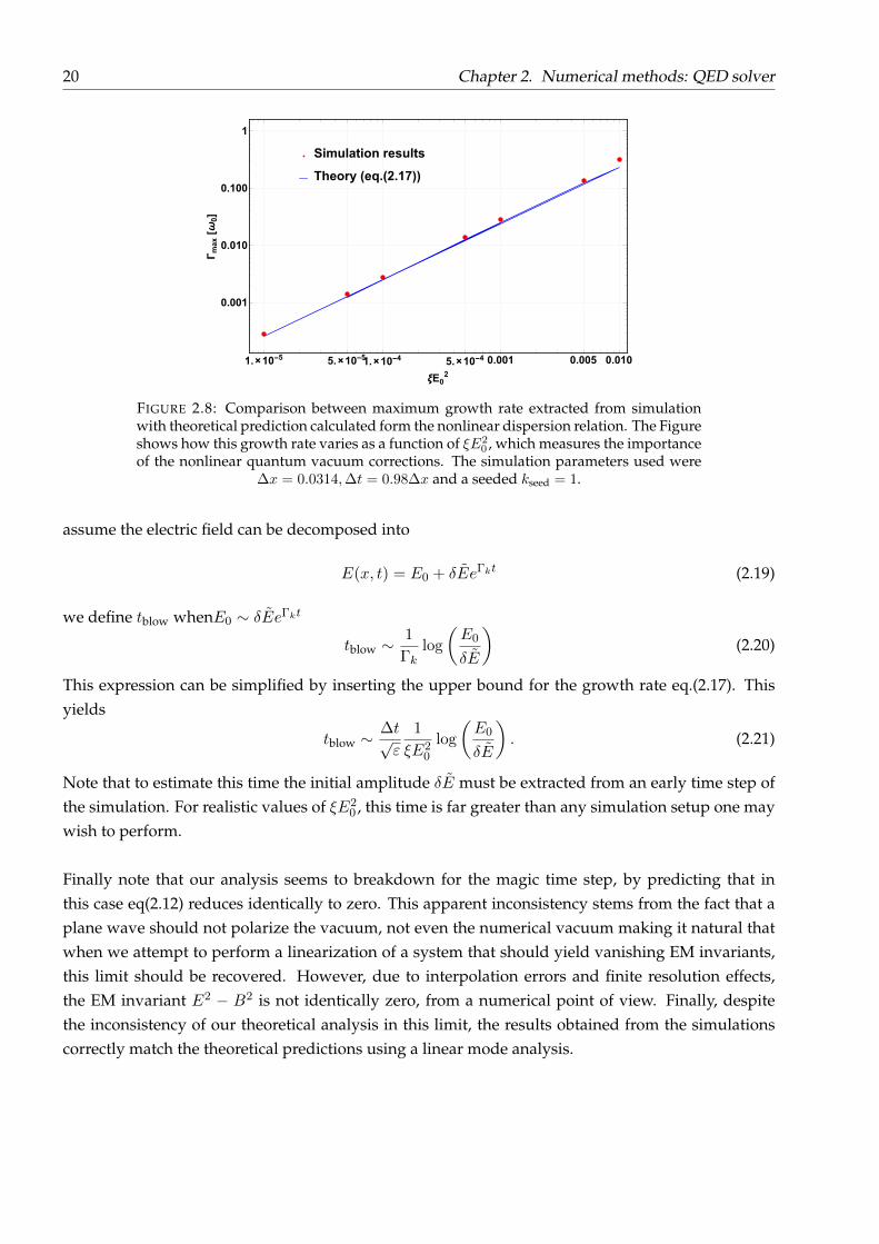
growing k-mode. . . . . . . . . . . . . . . . . . . . . . . . . . . . . . . . . . . . . . . . . 192.8 Comparison between maximum growth rate extracted from simulation with theoret-
ical prediction calculated form the nonlinear dispersion relation. The Figure showshow this growth rate varies as a function of ξE2
0 , which measures the importance ofthe nonlinear quantum vacuum corrections. The simulation parameters used were∆x = 0.0314,∆t = 0.98∆x and a seeded kseed = 1. . . . . . . . . . . . . . . . . . . . . . 20
2.9 Two-dimensional Yee grid cell combined with respective convention adopted for in-dexing within the code . . . . . . . . . . . . . . . . . . . . . . . . . . . . . . . . . . . . . 23
3.1 1D Gaussian pulse after an entire propagation over a periodic box in the presence of astrong static field, with (blue) and without (red) QED nonlinearities . . . . . . . . . . . 28
xii
3.2 (a) Phase velocity (c = 1) of probe pulse with polarization parallel to Es, (b) Phase ve-locity (c = 1) of probe pulse with polarization perpendicular to Es, both as a functionof ξE2
s parameter . . . . . . . . . . . . . . . . . . . . . . . . . . . . . . . . . . . . . . . . 293.3 Spatial Fourier transform of electric field with and without QED NL present. The
generation of odd higher harmonics can be observed in blue. . . . . . . . . . . . . . . 313.4 Temporal evolution of k = k0 Fourier mode of the subtracted electric field. . . . . . . 323.5 Simulation results of the phase velocity of a plane wave propagating in the x1 direction
in the presence of a strong static field, for different values of the quantum parameterξ. The corresponding prediction previously derived is plotted in red. . . . . . . . . . . 35
3.6 Initial setup of Gaussian pulses. Both pulses are polarized in the x2 direction and willfocus in the center of the box. . . . . . . . . . . . . . . . . . . . . . . . . . . . . . . . . . 36
3.7 Spatial Fourier transform of the electric field, (a) after the interaction but when QEDcorrections are absent, (b) after the interaction with self-consistent inclusion of thequantum corrections. k = 3k0 harmonics and small distortion of k = k0 can be ob-served. . . . . . . . . . . . . . . . . . . . . . . . . . . . . . . . . . . . . . . . . . . . . . . 36
3.8 Electric field setup for two Gaussian pulsed traveling in perpendicular directions butfocusing on the same point. . . . . . . . . . . . . . . . . . . . . . . . . . . . . . . . . . . 37
3.9 Spatial Fourier transform for E2 field at different stages of interaction. (a) Initial Fourierspace, if there were no vacuum nonlinearities this spectrum would remain unchangedthroughout the interaction. (b) At peak of nonlinear interaction when the pulses arecompletely overlapped in space. (c) Asymptotic state: after the nonlinear interactionthe pulses propagate independently but with higher harmonics generated from theinteraction. . . . . . . . . . . . . . . . . . . . . . . . . . . . . . . . . . . . . . . . . . . . . 38
4.1 Experimental setup proposed to study the birefringence of the quantum vacuum viathe change in the ellipticity of the polarization of a X-ray probe pulse, after trasversinga strong optical pump laser. . . . . . . . . . . . . . . . . . . . . . . . . . . . . . . . . . . 42
4.2 (a) Setup described in section 4.1.1 where a probe pulse polarized with an angle θ = π4
propagates in the presence of a strong static field, Es = 1000 (b) Result of polariza-tion diagnostic returned by the detector showing a line of gradient one but with asmall thickness caused due to the ellipticity induced in polarization of the pulse. (c)Polarization graph of the points presented in (b), rotated by θ = −π
4 as to center thecoordinate system such that the horizontal axis coincides with the major axis of theellipse, thus resolving the ellipticity in a more precise way. (d) The diagnostic finallyperforms a fit using the least squares method of the outer points of the ellipse to thegeneral quadratic equation for an ellipse, eq.(4.14). . . . . . . . . . . . . . . . . . . . . 46
4.3 Polarization plot showing the ellipticity induced in the polarization of the probe pulseafter propagating in a birefringent vacuum, caused by a strong static field, over a prop-agation distance d = 100. The labels a and b define the major and minor radii of thefitted ellipse respectively and are an output of the diagnostic developed. Using thesevalues we can extract the value of the ellipticity induced in the polarisation of thepulse, from the simulation. . . . . . . . . . . . . . . . . . . . . . . . . . . . . . . . . . . . 48

xiii
4.4 (a) 2D Contour plot of the field setup we wish to simulate. In this simulation wecounter-propagate a weak X-ray probe laser (traveling to the right) with a strong op-tical laser (traveling to the left). In the transverse direction there is no profile of thebeams, making this setup in practice quasi one-dimensional. (b) line-out for a constantx2 of the plot shown in (a) where we can see the longitudinal profile of each laser aswell as the difference in wavelengths . . . . . . . . . . . . . . . . . . . . . . . . . . . . . 49
4.5 Figure showing the results of the ellipticity diagnostic with the respective fit per-formed. In (a) the original polarization was rotated by θ = −π/4 where we see that theresidual angle that remains indicates the quantum interaction created a rotation in theoriginal direction of polarization. In (b) we show figure (a) but rotated once again bythis residual angle, measured from the diagnostic, to verify that the fitting parametersare invariant under coordinate rotations. . . . . . . . . . . . . . . . . . . . . . . . . . . . 57
4.6 (a) Figure comparing the ellipticities extracted from the simulations performed for dif-ferent values of the quantum coupling parameter. The points in blue and orange referto the results of the simulations using eqs.(4.42),4.41), respectively and are compared tothe theoretical expressions derived for the corresponding pump profile, eqs.(4.48,4.47),respectively. (b) Figure comparing the rotation of polarization angle extracted from thesimulations performed for different values of the quantum coupling parameter. Thepoints in blue and orange refer to the results of the simulations using eqs.(4.42),4.41),respectively and are compared to the theoretical expressions derived for the corre-sponding pump profile, eqs.(4.56,4.55), respectively. . . . . . . . . . . . . . . . . . . . . 59
A.1 Example of an arbitrary ellipse with the respective defining geometric parameters inthe general parametric form. . . . . . . . . . . . . . . . . . . . . . . . . . . . . . . . . . 72


xv
List of Tables
4.1 Laser parameters for the LCLSII update and the new SLAC X-ray laser. For the simu-lations performed for this setup all quantities were normalised to the X-ray frequency. 55


1
Chapter 1
Introduction
1.1 Vacuum
Vacuum, the Latin word for "an empty space", is a concept deeply rooted in many physical theories.This notion puzzled some of the greatest minds in History. Indeed, Aristotle and Plato themselvesargued that such a state of nothingness could not exist [1], whereas in the 13th century the notionof a true vacuum deeply conflicted with God’s omnipotence, as it was speculated that God wouldbe unable to produce vacuum [1]. It was not until the 17th century that Torricelli and Blaise Pas-cal demonstrated a partial vacuum in their famous experiments [1]. With the electromagnetic (EM)description of waves by Maxwell’s equations and the advances in thermodyanamics, the idea of aclassical vacuum seemed to be well established by the turn of the 19th century. However, this notionwas once again revolutionized by Paul Dirac in 1930 by proposing a vacuum filled with an infinitesea of electrons with negative energy [2]. This interpretation solved a delicate issue arising from thesolution of Dirac’s equation, known as the radiation catastrophe whereby if free states of negative en-ergy were to exist, then an electron in a 1s orbital, for example, could decay to a state of negativeenergy and from that state to one of even lower energy, until a state of −∞ energy thus making thehydrogen atom unstable. The infinite sea interpretation means that an electron from a negative en-ergy state could be excited by absorbing a photon with an energy equal to twice its rest mass, leavingbehind a "hole". The consequence of the "hole theory" was stated by Dirac [3]:
A hole, if there were one, would be a new kind of particle, unkown to experimental physics, having the samemass and opposite charge to an electron.
This was the first prediction of the existence of the positron, to be experimentally discovered in1932. The notion of a vacuum as a true state of emptiness was once again modified. In fact, QuantumElectrodynamics (QED) and many other quantum field theories, lend themselves to the same inter-pretation, making one thing clear: the so called "true" vacuum seems to be rich in dynamics, and nota static state of void. This realisation leads to astonishing physical consequences.
Heisenberg understood the deep implications of the hole theory and in 1934 published two semi-nal papers on the formalism behind the fluctuations of the quantum vacuum [4, 5]. Heisenberg alsoproposed that the fluctuations of electron-positron pairs could lead to a quantum nonlinear vacuum[5]. The exact nature of the nonlinearity of the quantum vacuum would become the PhD thesis of

2 Chapter 1. Introduction
Hans Euler, a student of Heisenberg. From their work resulted the conclusion that the vacuum couldbe polarized much like any other medium and that this effect could be taken into account, to leadingorder on the fine structure constant, as corrections to the Maxwell’s equations [6].
1.2 Motivation
The work developed by Heisenberg-Euler (HE) is known as the QED corrections to Maxwell’s equa-tions [6]. The HE model effectively treats the quantum vacuum as a medium whose response is takeninto account as extra polarization and magnetization terms in Maxwell’s equations. This formalismis extremely useful as it maintains the classical concept of EM fields instead of using the full sec-ond quantization formalism. This approach treats the electron-positron pair vacuum in the low fieldE � Es, low frequency ω � ωc, limit of the EM fields, where the Compton frequency is given byωc = mec
2/~ and the Schwinger critical field ESch = m2ec
3/e~. The Schwinger field has a value ofESch = 1.3 × 10¹⁸ V/m and was first identified by Sauter [7](although the idea is attributed to Born[8]) as the field strength at which one expects a Dirac sea electron to tunnel into the positive energycontinuum, thus polarizing the vacuum (with real particles).
The HE virtual polarization effect remains to be experimentally observed. However, with theexpected peak intensities, up to 1023 − 1024 Wcm−2, to be delivered by large scale facilities such asthe Extreme Light Infrastructure (ELI) or the VULCAN 20 PW project, the regime where these virtualfluctuations can be detected is finally within reach [9]. On the other hand, the existence of exoticastrophysical scenarios such as pulsar and neutron star magnetospheres, are known to contain suchextremely high field intensities [10] where these effects play an important role [11].
The main objective of this thesis is to develop an efficient numerical algorithm that can solve theHE modified Maxwell’s equations in a self-consistent manner. This tool is to be incorporated in themassively parallel, fully relativistic, Particle-in-Cell code (PIC) Osiris [12]. A PIC code can modelthe behaviour of multi-species plasmas, in the presence of strong EM fields, at the kinetic scale [13].Incorporating such a QED Maxwell’s equation solver in a PIC code provides an unique opportunityto study the dynamics of the quantum vacuum in any laser-laser interaction, as well as in plasmasof extremely high energy density dominated by EM fields. The scope of this work can, therefore, bedivided in three main areas:
- Develop a stable and robust algorithm to solve a set of nonlinear Maxwell equations in multi-dimensions.
- Benchmark and optimization of experimental setups aiming to detect the HE vacuum fluctu-ations for the first time using laser-laser interactions. A multi-dimensional self-consistent analysisshall be a novelty within the community.
- Reproduce, with simulations, existing predictions within the literature for several setups.

1.3. Theoretical framework 3
FIGURE 1.1: The fundamental QED vertex. This vertex is deduced from the QED La-grangian density when a coupling between a relativistic fermion and a EM field is in-cluded. The coupling constant is the electron charge e. Using combinations of the fun-
damental vertex, all interactions and processes in QED can be represented.
FIGURE 1.2: Feynman diagram of light-by-light scattering. This is the interaction thattriggers the virtual vacuum polarization. The naming of "virtual" polarization is due tothe fact that the electron-positron pairs are generated as internal fermionic lines in the
diagram
1.3 Theoretical framework
The theory of QED studies the interactions between fermions and photons using a relatively simplequantum field theory formalism. The theory of QED is one of the most successfully tested theoriesin physics, in the perturbative regime. As Richard Feynman so eloquently put it:
"If we measure the distance from New York to Los Angeles, the precision would be the thickness of a hu-man hair."
This statement is equivalent to a precision of 10−8. The fundamental QED vertex is shown in Fig.1.1and can be seen as the coupling of a fermion (electron in this case) with a quantum of the EM field(photon). The constant that couples these two fields is the fine structure constant α ≈ 1
137 . As DavidGriffiths states in his textbook when describing this fundamental vertex, [14],
"All electromagnetic phenomena are ultimately reducible to the following elementary process."

4 Chapter 1. Introduction
Using the fundamental vertex, and combinations of it, we can draw the respective Feynman dia-gram for each EM process. The HE QED corrections to Maxwell’s equations, physically represent thelowest order photon-photon QED interaction. The respective Feynman diagram is shown in Fig.1.2where it is clear that the photon-photon scattering is due to the polarization of the vacuum via apair of virtual electron-positron pairs (internal fermionic lines). In their 1936 paper [6], Heisenberg-Euler arrived at the expression for the full nonlinear correction to the Lagrangian of the EM field.Their result is derived from a non-perturbative calculation incorporating all orders in an uniform(background) EM field and can be found in the abstract of their paper:
L =e2
hc
∫ ∞0
dη
η3e−η
iη2(E ·B)cos(
ηESch
√E2 −B2 + 2i(E ·B) + c.c
)cos(
ηESch
√E2 −B2 + 2i(E ·B)− c.c
) + E2Sch +
η2
3(B2 − E2)
,
(1.1)WhereESch is the Schwinger field E,B the background electric and magnetic fields, respectively and ηa parameter introduced for convenience. The weak field expansion of the Lagrangian (|E|/ESch � 1),leads to the modified Maxwell Lagrangian, corrected to the lowest order in QED. This limit is thestarting point of this work,
L = ε0F + ξ(4F2 + 7G2) . (1.2)
where the effective coupling parameter for this interaction is given by
ξ =20α2ε2
0~3
45m4ec
5∼ 10−51 [Fm/V2] (SI) , (1.3)
and F and G are the two EM invariants, obtained from the Maxwell field tensor Fµν :
F =1
2(E2 − c2B2), G = c(E · B). (1.4)
The first term in eq.(1.2) yields the classical Maxwell’s equatons in vacuum whereas the remainingterms are the HE QED corrections. Re-writing these expressions in a covariant manner in terms ofthe field tensor is useful in order to derive the dynamical equations via the Euler-Lagrange equationsof motion. We therefore re-write the Lagrangian by noting that
F =1
2(E2 − c2B2) = FµνFµν , (1.5)
G = c(E · B) = −1
4GµνF
µν = −1
8εαβµνF
αβFµν , (1.6)
where εαβµν is the Levi-Civita symbol. In the theory of fields, the generalized coordinates (q,q), arereplaced by fields (functions of coordinates) and their derivatives [14]. In this case, the natural fieldto identify is the potential 4-vector Aµ, obeying the usual relation Fµν = ∂µAν − ∂νAµ. The Euler-Lagrange equations that will yield the modified Maxwell’s equations are thus:
∂L∂Aµ
− ∂ν(
∂L∂νAµ
)= 0. (1.7)

1.4. PIC method 5
This is a long but straightforward calculation analogous to the usual derivation of the covariantset of Maxwell’s equations. Although the resulting expression is fully covariant, its most useful formis when the indices are explicitly replaced (resulting in vector equations). The final result can bewritten as:
∂B∂t
+∇× E = 0 (1.8)
∇ · B = 0 (1.9)
∇× H− ∂D∂t
= 0 (1.10)
∇ ·D = 0 , (1.11)
withD = ε0E + P (1.12)
B = µ0H + M . (1.13)
Equations (1.8)-(1.13) are the usual Maxwell’s equations in a medium absent of real currents.The HE QED fluctuations manifest themselves as a nonlinear polarization and magnetization of thevacuum given by:
P = 2ξ[2(E2 − c2B2)E + 7c2(E · B)B
](1.14)
M = −2ξc2[2(E2 − c2B2)B− 7(E · B)E
]. (1.15)
It is evident from eq. (1.3) that the HE QED corrections to the Lagrangian are very small comparedto the usual Maxwell terms. This means that only in the presence of strong EM fields will thesecorrections be non-negligible, as is clear from the cubic field dependence of eq. (1.14) and eq. (1.15). An immediate and interesting feature of this theory is that for a plane wave, F = G = 0, meaningthat a plane wave is not affected by the HE nonlinearities.
The main objective of this thesis is to develop and optimize an efficient algorithm that can solvethis set of nonlinear Maxwell equations whilst incorporated in a massively parallel PIC code. We willnow briefly describe how the PIC method works and what are it’s main advantages.
1.4 PIC method
The PIC method consists of self-consistently solving the equations of motion for all the particles ina discretized spatial grid and it is ideal to study kinetic scale phenomena [13]. Each macro particle(representing an ensemble of real particles) is initialized in the grid. The charge and current densitiesare then deposited at the edges of the grid-cells, from which the electric and magnetic fields are com-puted by Maxwell’s equations. The fields are interpolated back to the positions of the particles, andthese are updated in time by integrating the relativistic Lorentz equation of motion. By modifyingthe algorithm that solves Maxwell’s equations to include QED vacuum fluctuations effects, the PICmethod ensures that the single particle dynamics will evolve according to the QED corrected, self-consistent, EM fields.

6 Chapter 1. Introduction
PIC codes can be used in a variety of contexts traditionally ranging from laser-plasma interaction,to plasma instabilities or even to study Inertial confinement fusion (ICF). On the other hand, the in-creasing consensus regarding the importance of quantum dynamics in the collective effects of manyextreme laser plasma systems has motivated the development of novel numerical tools that couplethe multiple scales associated with the problem. Numerical codes that simulate quantum radiationreaction [15–17] and pair production effects [18–22], have already made important predictions inextreme energy density scenarios [22–24]. However, a method to include the effect of vacuum polar-ization via the creation of virtual pairs, in multi-dimensions and for a broad set of initial conditions,has not been proposed yet. In particular, the ability to fully self-consistently couple the dynamics ofrelativistic particles with the various ultra-high intensity processes with vacuum polarization effectshas not been accomplished.
1.5 State of the Art
Vacuum polarization, via the fluctuation of virtual electron-positron pairs, remains to be detectedexperimentally. In recent years, this topic has motivated great interest in light of the possibility ofdetecting the dynamics of the quantum vacuum with the development of new laser facilities [25]. Athorough and complete review on the topic of strong field QED in the context of laser interactions byDi Piazza et al. may be found in [26].
The fundamental dimensonless parameter used to describe a laser amplitude, a0, is defined as,
a0 =eEλ0
mec2, (1.16)
representing the normalised laser vector potential and also standing for the classical ratio of theenergy gained by an electron traversing the laser field E across a laser wavelength λ0. For a laserwavelength in µm, the relation between a0 and the intensity is
a0 =
√I[W/cm2]λ
20[µm]
1.37× 10¹⁸(1.17)
Table 1 in [25], compares the expected intensities and respective a0 of existing and future plannedlaser facilities. In that table a clear emphasis goes to the ELI and Vulcan projects estimated to deliverpeak intensities of 1025 and 1023 W/cm2 with 1 µm wavelength radiation corresponding to a a0 of 200and 5000, respectively. Combining Eq.(1.3) with Eq.(1.16), a useful relation can be derived to obtainthe order of the HE corrections compared to unity,
LHELQED
=ξE2
ε0∼ 6× 10⁻²³[µm]2
a20
λ20[µm]
. (1.18)
Eq.(1.18) serves as a quick estimate for the relevance of the HE QED corrections in a given setup.

1.5. State of the Art 7
From a theoretical point of view, diverse setups have been considered in order to explore thesecorrections. A brief overview shall be given here. An immediate consequence of the modified HEQED Maxwell equations is that in the presence of a strong static field a probe pulse will propagatein vacuum with an index of refraction n 6= 1, leading to vacuum birefringence [27]. In particular, astrong static field will induce a very small ellipticity on a probe pulse with initial linear polarization.The PLVAS experiment [28], aims to detect such an effect using a high finesse (> 2×10⁵) Fabry-Perotcavity and two permanent magnets of 2.5 T. The expected change in the index of refraction of theEM wave propagation in vacuum can be calculated to be ∆nQED = 2 × 10⁻²³, indeed an extremelysmall quantity. In 2012, the experiment described in [28], has placed an upper limit on the value ofthe fundamental coupling constant of the interaction, Eq.(1.3), of ξ < 2.85× 10−49.
The development of Chirped Pulse Amplification (CPA) has allowed for both the power and theintensity of lasers to grow at a steady rate. This technological development inspired a different ap-proach to detect the effects of vacuum polarization as pointed by Di Piazza et al. [29]. In their analysisthe interaction between a linearly polarized x-ray probe beam and a focused, intense standing laserwave was proposed and studied theoretically, giving rise to diffraction effects of the probe pulseand leading once again to both a polarization rotation angle and an induced ellipticity. This setup,however, is far more complex from a theoretical point of view due to finite spot size transverse ef-fects and pulse dynamics. The full complexity can only be captured with numerical simulations thusmaking this setup very interesting to simulate with the computational tool to be developed in thisthesis. Compared to the PLVAS experiment, it is estimated that such a setup can induce an ellipticity2 orders of magnitude greater [29]. Furthermore, this method is single passage in the sense that itdoes not require an optical cavity as in PLVAS. A similar experimental setup in the framework of theHelmholtz International Beamline for Extreme Fields (HIBEF), is currently being planned at DESY(Deutsches Elektronen-Synchrotron) [30].
Other exotic setups have also been proposed. In 2000, M.Solijacic and M.Segev [31] showed thatin a full 3D setup the HE QED Maxwell equations support nondiffracting spatial radiation solitonsthat can propagate for very long distances without changing their shape. These solitons present anexciting physical system to be studied in future experiments and clearly a 3D simulation of such asetup would further motivate its implementation. In 2013, B.King, Di Piazza and C.Keitel, proposeda double slit-like experiment where two ultra-intense Gaussian pulses are tightly focused and an (al-most) antiparallel probe beam of much wider spot size is counterpropagated leading to a diffractionpattern as shown in Fig. 1.3. This setup was named the Matterless Double Slit [32]. Finally, in ref [33]the existence of new modes generated within a waveguide was shown and this was proposed as away to detect the QED nonlinearities [33], using technology currently available with state-of-the-artbut relatively modest field strengths E ≈ 30 MV/m.
A few efforts have been aimed at developing the computational tools to self-consistently solvethe HE QED Maxwell equations. The first algorithm was developed in 2014 in [34]. In that work,limited to 1D academic setups, it was shown that by interacting two colliding plane wave pulses(with different parameters), higher harmonics of the original probe pulse are generated. An analytictreatment was performed by solving the corresponding wave equation. The numerical method usedin this work is one dimensional and involves matrix inversions to solve the modified Maxwell’sequations. In principle this method could be extended to higher dimensions. However, not only does

8 Chapter 1. Introduction
Figure 1: A matterless double-slit set-up. Two ultra-intense Gaussian laser pulses with wavevec-
tors ks,1 and ks,2 are tightly focused by the lenses L1 and L2 (almost) antiparallel to a probe beam
with wavevector kp of much wider spot radius (see also inset a)). The vacuum current, activated in
the interaction regions of the probe and the strong laser fields, generates photons which interfere
to produce a diffraction pattern on the screen S. The screen is placed between the focusing mirrors
at a distance y along the propagation axis of the probe from the interaction centre and has a hole
in the centre allowing the probe beam to pass undisturbed (see also inset b)). The directions of the
spatial co-ordinates x, y, z and the angle θ between the strong field Es and the probe field Ep are
defined in the inset a).
5
FIGURE 1.3: Matterless double slit setup: lenses L1 and L2, focus two ulta-intense gaus-sian pulses are counterpropagated at a small and symmetric angle to a probe pulse witha much larger waist leading to an interference pattern in the screen S (b). Figure 1 in
original article [32]
the computational demand increase significantly, but also, the nature of this scheme is not adequatewithin the usual PIC algorithm. The algorithm to be developed in this thesis is an alternative tothis method, being an extension of the Yee algorithm which is finite difference in nature. It should bementioned that, in [34], higher order multi-photon QED corrections are taken into account for the onedimensional setup proposed. These higher order corrections are shown to create a steepening of theprobe pulse, an effect named as an "Electromagnetic shock". Although the higher order correctionsare not within the scope of this thesis, it is expected that the numerical tool developed in this thesiscan be extended in a straightforward manner to include such effects.
A final note regarding an extremely comprehensive and complete review of the Heisenberg-Eulereffective action by G.Dunne can be found in [8]. This procedings paper covers the talk given atthe conference QFEXT11 commemorating the 75th anniversary of the original HE publication, andit provides an excellent historical review on the topic and a complete overview on the formalismbehind the HE QED corrections and how it can be derived in alternative manners such as via theFeynman-Schwinger proper time formulation.

9
Chapter 2
Numerical methods: QED solver
Maxwell’s equations modified by the Heisenberg-Euler quantum vacuum corrections constitute a setof nonlinear partial differential equations. The objective of this chapter is to explain the numericalalgorithm developed to solve this new set of nonlinear equations numerically in multi-dimensionsand for a broad set of initial conditions. The chapter is organized as follows: we start, in section2.1, with a brief description of the Yee scheme, a finite difference algorithm to solve the set of linearMaxwell’s equations. In section 2.2 we present our QED solver as a generalization of the Yee schemeto a nonlinear system and explain each step of the algorithm in detail. In section 2.3 we explainhow to perform a numerical stability analysis and generalize the usual linear mode analysis to ournonlinear solver. Finally, in section 2.4 we discuss some of the details of how the algorithm wasincorporated in the PIC code Osiris, in an user guide approach.
2.1 Maxwell equation solver: Yee Scheme
2.1.1 Summary
A standard finite-difference time domain (FDTD) method to solve Maxwell’s equations is the YeeAlgorithm [35]. The Yee scheme, to be described below, solves simultaneously for both electric andmagnetic fields by solving Faraday’s and Ampère’s law, respectively. The explicit linear dependenceof Maxwell’s equations on the fields allows the field solver to be centered both in space and time (leapfrog scheme), thus providing a robust, second order accurate scheme without the need to solve forsimultaneous equations or matrix inversion [36]. Moreover, the efficiency and simplicity of the Yeescheme allows an easy incorporation into numerically parallel PIC codes. Following [36], we will gothrough the essentials of the Yee scheme, from what it means to discretize a differential equation, tothe problems that the algorithm offers when adding the QED corrections to Maxwell’s equations.

10 Chapter 2. Numerical methods: QED solver
2.1.2 Numerical discretisation of Maxwell equations
The Yee scheme solves the Maxwell’s equations using a numerical method called finite-differencetime domain (FDTD). The Maxwell’s equations in vacuum, can be written in a vector form as
~∇ · ~E = 0, (2.1a)~∇ · ~B = 0, (2.1b)
~∇× ~B − 1
c2
∂ ~E
∂t= 0, (2.1c)
∂ ~B
∂t+ ~∇× ~E = 0 , (2.1d)
where eqs.(2.1c-2.1d) are the time-dependent equations dictating the dynamics of the EM fields,whereas the divergence equations, eqs.(2.1a-2.1b) serve as constraints that must be valid at all times.Furthermore, it can be easily shown that eqs.(2.1a-2.1b) are not independent from eqs.(2.1c-2.1d),meaning that by solving the time-dependent equations for the fields in a self-consistent way, thedivergence equations will automatically be satisfied for all times. Kane Yee in 1966, derived a setof finite difference equations from eqs.(2.1c-2.1d) to advance the electric and magnetic field in time,respectively. The accuracy and robustness of Yee’s algorithm comes from the discretisation of theequations in both time and space combined with the linearity of the equations themselves. The al-gorithm benefits from second order accuracy due to the fact that the fields are centered both in timeand in space, as we shall now explain.
To illustrate this in a one-dimensional example, we start by writing (2.1c-2.1d) in an explicit com-ponent form. The one-dimensionality of the problem means that there can only be non-zero deriva-tives in one spatial direction (in this case, the x-direction), even though the EM fields can be definedin all three Cartesian directions. This yields:
∂tEx = 0 (2.2a)
∂tEy = −c2∂xBz (2.2b)
∂tEz = c2∂xBy (2.2c)
∂tBx = 0 (2.2d)
∂tBy = ∂xEz (2.2e)
∂tBz = −∂xEy , (2.2f)
let the indexes i and n denote the spatial and temporal discretised position on the grid respec-tively. In this notation, an electric field evaluated at position x = i∆x and at time t = n∆t is denotedby E(x, t) = Eni . We are now in a position to discretise eqs.(2.2a-2.2f) along the x-direction in one-dimension (meaning there can only be derivatives in the x-direction). The spatial grid on whicheqs.(2.2a-2.2f) are discretised is shown in Fig.2.1 where we emphasize the fact that the electric andmagnetic fields are not evaluated in the same spatial positions, but instead are displaced by half acell (from i to i+1/2). This illustrates a crucial feature of the Yee algorithm: the fact that the fieldsare de-centered in space. The importance of this de-centering can be understood by looking at thesystem of equations (2.2a-2.2f), where we see that in order to advance a field at a given point (time

2.1. Maxwell equation solver: Yee Scheme 11
derivative term), the spatial derivative of the other field must be computed. However, since calculat-ing a spatial derivative of a field involves evaluating the values of the field at nearby points, the griddisposition shown in Fig.2.1, makes this derivative correctly centered in space as the required fieldsare only displaced by ∆x/2 to either side. Furthermore, the Yee algorithm is also correctly centeredin time meaning that to advance a field from time step n to n+1, using the system (2.2a-2.2f), the spa-tial derivatives terms are not only shifted in space by ∆x/2, but are also evaluated at the time stepn+1/2. Again, this shift in time by half a step, of the fields, allows the Yee scheme to be second-orderaccurate in time and is known as a leap-frog configuration.
FIGURE 2.1: One dimensional spatial grid illustrating the disposition of the electric andmagnetic fields. This illustrates the fact that the both fields are staggered both in space
and in time
The concepts just described, become clear when explicitly discretising the system (2.2a-2.2f). Asan example, eqs.(2.2b,2.2f) are discretised below. Together, these equations self-consistently accountfor the temporal evolution of the Ey and Bz field components. This discretisation yields:
En+1y i − Eny i
∆t= −c2
Bn+1/2z i+1/2 −B
n+1/2z i−1/2
∆x
, (2.3a)
Bn+1/2z i+1/2 −B
n−1/2z i+1/2
∆t= −
(Eny i+1 − Eny i
∆x
). (2.3b)
The numerical scheme is finalized by taking eqs.(2.3a-2.3b), and rearranging as follows,
En+1y i = Eny i −
c2∆t
∆x(B
n+1/2z i+1/2 −B
n+1/2z i−1/2) (2.4a)
Bn+1/2z i+1/2 = B
n−1/2z i+1/2 −
∆t
∆x(Eny i+1 − Eny i). (2.4b)
Eqs.(2.4a,2.4b) are complete in describing the self-consistent evolution of the fields Ey and Bz , butalso illustrate the concepts of spatial and temporal centering of the fields. This is clear by noting thatto evolve any quantity from time step n to n + 1, this is done by incrementing the field at the sameplace at time step n, by the other field evaluated at time step n+1/2 and at adjacent spatial positions.It is straightforward to repeat this process for the equations for the remaining field components andin higher dimensions due to the linearity of the system of equations.
A more complete discussion and generalization of the Yee Scheme in multi-dimensions can befound in chapter 3 of [36], in particular the beautiful relation between how the EM fields are disposed

12 Chapter 2. Numerical methods: QED solver
within a 3D spatial grid cell, and the physical meaning of Maxwell’s equations in the differentialform.
2.2 QED solver: generalized Yee scheme
To solve the QED Maxwell equations, a modified Yee scheme was developed to address the two maindifficulties which arise from the nonlinear polarization and magnetization of the vacuum, eqs.(1.14-1.15). The first difficulty is a direct consequence of the loss of linearity in the modified Maxwell’sequations. To understand this difficulty, we recover the one-dimensional example from sec.2.1 andre-write eqs.(2.3a,2.3b) including the nonlinear quantum vacuum terms
En+1y i − Eny i
∆t+Pn+1y i − Pny i
∆t= −c2
Bn+1/2z i+1/2 −B
n+1/2z i−1/2
∆x
+1
µ0
Mn+1/2z i+1/2 −M
n+1/2z i−1/2
∆x
(2.5a)
Bn+1/2z i+1/2 −B
n−1/2z i+1/2
∆t= −
(Eny i+1 − Eny i
∆x
). (2.5b)
To complete the numerical algorithm in a self-consistent way including the vacuum polarizationand magnetization, we would have to rearrange eqs.(2.5a-2.5b) to isolate the terms for En+1 andBn+1/2, respectively. However it is clear that this is no longer possible as the polarization termevaluated at time step n + 1 is a nonlinear function of all EM field components at n + 1, which areexactly the quantities we wish to compute. This example illustrates how the nonlinearity introducedin Maxwell’s equations due to the HE corrections, no longer allows the use of the Yee algorithm toadvance the EM fields in time in a straightforward manner.
The second difficulty that arises when attempting to apply the Yee algorithm to the Maxwell’sequations corrected by the HE QED terms, is the fact that the nonlinear polarization and magne-tization terms depend on the EM invariants E2 − B2 and ~E · ~B. Both these quantities require theknowledge of all the fields in every grid position as opposed to the usual spatially staggered fieldconfiguration described in the previous section. This is a significant obstacle regarding the essenceof the Yee scheme as the algorithm may no longer be correctly spatially centered.
The two main problems that arise when attempting to apply the Yee scheme to the nonlinearset of QED Maxwell’s equations are therefore the fact that the modified Ampère’s law requires theknowledge of future fields and the need to know the value of all field components in every gridposition to calculate the polarization and magnetization of the vacuum. The former difficulty servedas the main motivation to develop our modified Yee scheme. The steps of the algorithm we proposeare illustrated in Fig.2.2 and shall now be described for a time step ∆t:
– we begin by advancing the fields using the standard Yee scheme (i.e. without accounting forthe polarization and magnetization of the vacuum). This setup allows us to obtain predictedquantities for the values of the fields at the new time. This approach is based on the standardtechnique of the predictor-corrector method, where the linear Maxwell equations are solved asthe zeroth order solution to the fields;

2.2. QED solver: generalized Yee scheme 13
– the predicted field values are then interpolated at all spatial grid points using a cubic splineinterpolation method thus allowing to calculate quantities such as the EM invariants and re-spective polarization and magnetization of the vacuum, to lowest order;
– the polarization and magnetization are then used to advance the electric field via the modifiedAmpère’s law;
– the convergence loop re-injects this new electric field value back into the polarization and mag-netization source terms to refine these quantities and re-calculate the electric field iteratively.This loop is reiterated until the electric converges to a value within the desired accuracy;
– after convergence is achieved, Faraday’s law is advanced, identically to the linear Yee scheme,benefiting from the fact that the electric field values being used are self-consistent with the QEDcorrections.
Start
FIGURE 2.2: Full loop of the modified Yee scheme
It must be emphasized that this method is only valid as long as the effects of the polarization andmagnetization of the medium are small compared to the non-perturbed propagation of the fieldsgiven as solutions to Maxwell’s equations in classical vacuum. This condition is automatically sat-isfied for realistic values of electromagnetic fields available in current, or near future, technology.In this regime, the QED theory is valid since the Schwinger field, above which the production ofreal electron-positron pairs is possible, corresponds to an electric field of ESch ∼ 1018V/m, whereasambitious laser facilities aim to push available intensities to the 1023 − 1024 W/cm2 (E ∼ 1015V/m)range. The order of the ξ parameter in eqs.(1.3,1.14,1.15) clearly helps to ensure the validity of themethod. Therefore, this scheme highly benefits from the fact that the nonlinear QED corrections ofthe vacuum are perturbative in nature. The convergence loop can be seen as a Born-like series sincefor every re-insertion of the fields back into the nonlinear source term, there is a gain in accuracy ofone order in the expansion parameter to the result. The algorithm proposed here solves Ampère’slaw by treating the nonlinear corrections as a source term, in an iterative manner,
~∇× ~B − ∂t ~E = ~SNL[E,B], (2.6)
where ~SNL = ~∇× ~M+∂t ~P . From this discussion and eq.(2.6), we can conclude that this generalizationof the Yee scheme can be extended beyond the framework of QED corrections to the vacuum as

14 Chapter 2. Numerical methods: QED solver
it is valid to solve Maxwell’s equations in any nonlinear medium provided that the polarizationand magnetization are given and that their order is such that they can be treated as a perturbation.This possible generalization enhances the range of applicability of our algorithm. Furthermore, theinclusion of a current in the algorithm (J 6= 0 in Ampère’s law) can be done, both within a PICframework or for a macroscopic field dependent current by including the current term in the initialstandard Yee scheme loop where the predictor quantities are computed. This is another key featureregarding the ability to couple our proposed generalized Yee solver to the PIC framework.
2.2.1 Interpolation of the fields
The algorithm requires that all fields are calculated at the same spatial positions. When consideringthe spatial interpolation of the self-consistent fields given by the Yee Algorithm we found a clearasymmetry between interpolating the electric field at the magnetic field position or vice-versa interms of the precision of the EM invariant E2−B2 for both cases. Since a plane wave is a trivial solu-tion of the QED Maxwell equations, the invariants calculated in the simulation should be identicallyzero [37]. Figure 2.3 shows the distribution of the EM fields within a two-dimensional Yee grid cell.We found that all the standard interpolation schemes yield invariants with much greater precisionat the lower left corner of the cell compared to the other positions. This difference in precision wasfound to be of two orders of magnitude when tested for a plane wave in 1D, which can affect thestability and precision of the code. The reason for this artifact is due to the way that the fields areinitialized within the simulation domain. In particular, the fact that the electric and magnetic fieldsmust be initialized with a shift both in space and time, creates an asymmetry between interpolatinga field to the corresponding position of the other field, even if this interpolation is done in a centeredmanner. The solution we have adopted to address this problem is to calculate all the fields at the cellcorner where the invariants are known to be of higher precision. For instance, the Bz component atthe left corner of the cell becomes
Bz i,j = I(Bz i+ 12,j+ 1
2, Bz i− 1
2,j+ 1
2, Bz i+ 1
2,j− 1
2, Bz i− 1
2,j− 1
2),
where I is an interpolation function. Once all fields are calculated at the (i, j) positions, we cancompute the invariants at these positions and then re-interpolate these invariants directly to the othergrid cell points in a similar fashion. The correct calculation of the EM invariants is necessary in orderto evaluate the nonlinear polarization and magnetization of the vacuum via eqs.(1.14-1.15)
Having proposed a generalized Yee algorithm and explained in detail the algorithm along withits subtleties, we now move on to analyse the numerical stability properties of the algorithm. Themotivation in performing this study is to investigate whether the algorithm is ultimately stable underthe same conditions as the linear Yee algorithm , and if not, what parameters of the simulation canbe used to control the stability in order the ensure the results obtained are physically meaningful inthe desired regimes.

2.3. Algorithm Stability: linear and nonlinear analysis 15
FIGURE 2.3: Two-dimensional Yee grid cell
2.3 Algorithm Stability: linear and nonlinear analysis
The method adopted to study the numerical stability of the QED polarization solver follows thestandard mode analysis [36]. This method involves linearizing the discretized set of equations usinga Fourier mode analysis. For the QED corrected Maxwell’s equations, this amounts to introducingthe following dependence for the EM fields
E = Ee−jωt+jkx (2.7)
B = Be−jωt+jkx, (2.8)
where E and B, represent the amplitudes of a given ω, k pair that satisfy the appropriate dispersionrelation, to be identified. This representation of the fields can be discretized on a one-dimensionalstaggered grid, using the notation from 2.1, yielding,
Eni = Ee−jωn∆t+jki∆x (2.9)
Bn+1/2i+1/2 = Be−jω(n+1/2)∆t+jk(i+1/2)∆x, (2.10)
Inserting eq.(2.9) and eq.(2.10) into the linear set of Maxwell’s equations yields the numerical disper-sion relation that is to be expected for a plane wave propagating on a grid with spatial and temporalresolution ∆x and ∆t, respectively, is [36]
ω0 =1
∆tarccos
(1 +
(c∆t
∆x
)2
(cos(k∆x)− 1)
). (2.11)
A notable case is when ∆t = ∆x/c for which eq.(2.11) reduces to the EM dispersion relation for aplane wave in vacuum, ω0 = ck. To study the stability of the new set of QED-corrected Maxwell’sequations using this method, a self-consistent numerical dispersion relation was derived. Due to thenon-linearity of the equations, the new dispersion relation can be written as(
c∆t
∆x
)2
sin
(k∆x
2
)2
− sin
(ω∆t
2
)2
= ξE20FNL(ω, k,∆x,∆t), (2.12)
where E0 is the amplitude of the wave and FNL is a nonlinear function of ω, k, and the spatial andtemporal steps. In the classical limit ξ → 0 the RHS goes to zero and the dispersion relation reduces

16 Chapter 2. Numerical methods: QED solver
to eq.(2.11). The explicit form of the nonlinear function FNL is given by
FNL = Inv(k, ω)exp(−2jφ)
[(∆t
∆x
)2
sin
(3∆xk
2
)sin
(∆xk
2
)− sin
(3∆tω
2
)sin
(∆tω
2
)](2.13)
Where φ = −(n + 1/2)ω∆t + k∆xi and Inv(k, ω) represents the Fourier amplitude defined byInv(k, ω) = (E2 − B2)(k, ω). A numerical plane wave propagating via our QED solver will there-fore obey eq.(2.12).
Eq.(2.13) explicitly shows a great difficulty that arises from attempting to perform a linear nu-merical stability analysis on a nonlinear system of equations: the fact that the dispersion relationdepends on both spatial and temporal grid indices i and n, respectively. This, combined with theexponential function with imaginary argument, appears to show that the dispersion relation of aninitialised plane wave will depend on the spatial and temporal positions on the grid. This representsa clear sign of instability and chaotic dynamics. On the other hand, the fact that the left-hand sideof eq.(2.12) is a small correction to the linear dispersion relation, hints that this nonlinear behaviourdiscussed will only be a higher order correction. To make the analysis possible, we assume that thedispersion relation cannot depend on the spatial and temporal indices and therefore we perform thefollowing replacement in eq.(2.13),
exp(−2jφ)→ 1√2
(1 + j) (2.14)
This approximation will later be verified by the results obtained. However, the reasoning behind ourapproximation is that the exponential term creates a unpredictable phase that slightly modifies theamplitude of the corrections to the linear dispersion relation with a factor that is varying in time andspace. By taking this approximation, we are essentially taking the upper limit of this random phase,meaning that we are still capturing the important aspects of the numerical stability of the system.
To continue the analysis, we have to calculate the value of Inv(k, ω) for the numerical plane waveintroduced in the system. For a numerical plane wave the EM invariant ~E · ~B is identically zero,whereas the invariant E2 − B2 will not vanish identically due to finite spatial resolution and thefact that the fields must be interpolated in space to evaluate the invariants, as already discussedabove. Therefore, the amplitude of this EM invariant depends on the interpolation method and gridresolution. We calculate this dependence by evaluating E2 − B2 at a given grid point, taking intoaccount that a correct centering in space implies one of the fields must be interpolated to the positionof the other. Interpolating the B field using linear interpolation is formally equivalent to computing
(E2 −B2)ni = E2i −B2
i = E2i −
(Bi+1/2 −Bi−1/2
2
)(2.15)
Having evaluated this EM invariant on a grid position using correctly centered fields, the final step isto substitute the amplitudes eqs.(2.9-2.10) and replace the magnetic field amplitude using Faraday’slaw. After some algebra this finally yields
Inv(k, ω) = E20
[1− sin2(k∆x/2)
sin2(ω∆t/2)cos2
(k∆x
2
)]. (2.16)

2.3. Algorithm Stability: linear and nonlinear analysis 17
This expression was compared to the results extracted from one-dimensional simulations. The simu-lation setup comprised of a 1D periodic box initialised with a plane wave of amplitude E0, such thatthe wavelength of the wave is a multiple of the box size. We repeated this simulation using differ-ent initial wavelengths corresponding to different seeded k modes. Figure ?? shows a comparisonbetween eq.(2.16) and simulations with several seeded k modes and with ξE2
0 = 10−4 , ∆t = 0.98∆x
and ∆x = π/100.
●
●
●●
●
●
●
●
●
●
●
●
Theory (eq.(2.16))
● Simulation
0 10 20 30 40 50
0.001
0.010
0.100
1
k [ω0/c]
Invariant[E02]
FIGURE 2.4: Amplitude of EM invariant E2−B2 as a function of the seeded k-mode fora resolution ∆x = π/100, ∆t = 0.98∆x and ξE2
0 = 10−4. Simulation results in blue arecompared to eq.2.16 in red.
The simulation points agree with the trend presented by the theoretical curve. This result showsthat eq.(2.16) provides an upper bound to the interpolation error when seeding a particular k mode.In particular, the results show that for higher wave numbers, up to the resolution limit, the order ofmagnitude of the invariant amplitude increases, tending towards unity. One shall therefore limit thesimulations to low k modes in order to insure the smallness of the invariants.
The stability of the QED Yee solver, i.e., the nonlinear dispersion relation, eq.(2.12) was solvedusing three methods: a numerical solution, an analytical solution through the linearization of thesystem via the ansatz ω = ω0 + δω with δω � ω0, and finally by estimating the growth rate of themaximum mode allowed by the grid resolution i.e. k∆x = π. The results are shown in Fig. 2.5 forsimulations performed with a grid resolution of ∆x = 0.0314, ∆t = 0.98∆x and ξE2
0 = 10−4.One can verify in Fig.2.5 that the analytic solution is in excellent agreement with the numerical
integration. The maximum growth rate is given by
Im(δωmax) ' 2ξE20
√8ε
∆t, (2.17)
where ε = 1− ∆t∆x . The maximum growth rate predicted theoretically serves therefore as an accurate
rule-of-thumb criteria to understand how unstable a given simulation setup may be. Finally we tookthe solution of the perturbative expansion and studied the limit for small k values, which yields
limk∆x→0
Im(δω) =1
4
ξE20(k∆x)5
∆x. (2.18)

18 Chapter 2. Numerical methods: QED solver
FIGURE 2.5: Imaginary part of solution of nonlinear dispersion relation, eq.(2.12), as afunction of k-mode, calculated using three different methods. Simulation parameters
used were ∆x = 0.0314, ∆t = 0.98∆x and ξE20 = 10−4.
Eq.(2.18) suggests that the smallest k modes will be ultimately stable as, not only does the growthrate scale with the small quantity ξE2
0 , but also due to the power law applied to the small value ofk∆x. This is an important result since, in principle, the low k modes, for a given grid resolution, arethose that will be seeded for a simulation setup.
These theoretical predictions were compared with one-dimensional simulations by extracting thegrowth rate of a given k mode in the simulation domain. The process to extract this maximumgrowth rate was the following: after completing the simulation with a seeded k mode, we applied adiagnostic that shows the amplitude of each k mode as a function of time. An example this diagnosticfor a given simulation is shown in Fig-.2.6 where we can see that the higher k-modes are those thathave a more dynamic growth after a certain critical time. In Fig-2.6 we can also see a horizontal lineat a low k value that corresponds to the seeded mode.
To extract the maximum simulation growth rate, we perform a horizontal line-out by choosingthe k that achieves the highest amplitude. In Fig.2.6 this happens for k = 83, and the correspondingline-out is shown in Fig.2.7. In Fig.2.7, we observe a transient period of no growth in the fields beforethe onset of the linear growth phase, after which there is a period of linear growth. Finally, oncethe amplitude of the unstable k modes become comparable to that of the initial seeded mode, thereis a blow-up of the fields and consequently and increase in EM energy at a rate far greater than anexponential. Finally, to measure the maximum growth for this simulation one must take the gradientof linear section in Fig.2.7.
The results for the maximum growth rate extracted are shown in Fig.2.8. The growth rate was ex-tracted from the Fourier spectrum of the simulations for different values of ξE2
0 . Figure 2.8 shows aclose agreement between the maximum growth rates extracted and eq.(2.8). Our theoretical analysisshows that the growth rate of the most unstable mode scales linearly with ξE2
0 . Furthermore, we

2.3. Algorithm Stability: linear and nonlinear analysis 19
FF
T -
k [a.u
.]
80
60
40
20
0
time [ ω p
-1]
800006000040000200000
FFT vs Time
FF
T v
s T
ime [a.u
.]
100
10-2
10-4
10-6
10-8
FIGURE 2.6: Amplitude of each k mode as a function of time.
FF
T a
mp
litu
de
10-2
10-4
10-6
10-8
10-10
time [ ω p
-1]
1× 10⁵
8× 10⁴
6× 10⁴
4× 10⁴
2× 1040
k = 83.500000
FFT vs Time
FIGURE 2.7: Line-out at k = 83 from Figure 2.6 to extract the temporal evolution of thefastest growing k-mode.
performed simulations under the same conditions, varying only the seeded k mode and verified thatthis does not affect the growth rate of the most unstable high k modes. Instead, it is the amplitude ofthe seeded mode that affects the growth rate of the higher k modes by nonlinear coupling.
The transient time between the onset of the linear growth phase and the blowup can be estimatedby assuming this blow-up occurs once the amplitude of the fastest growing k-modes δE (initiallythis amplitude is at the numerical noise level, and can be measured from the initial spectrum of thefields in the simulation), become of the order of the initial seed amplitude. To estimate this time, we
20 Chapter 2. Numerical methods: QED solver
FIGURE 2.8: Comparison between maximum growth rate extracted from simulationwith theoretical prediction calculated form the nonlinear dispersion relation. The Figureshows how this growth rate varies as a function of ξE2
0 , which measures the importanceof the nonlinear quantum vacuum corrections. The simulation parameters used were
∆x = 0.0314,∆t = 0.98∆x and a seeded kseed = 1.
assume the electric field can be decomposed into
E(x, t) = E0 + δEeΓkt (2.19)
we define tblow whenE0 ∼ δEeΓkt
tblow ∼1
Γklog
(E0
δE
)(2.20)
This expression can be simplified by inserting the upper bound for the growth rate eq.(2.17). Thisyields
tblow ∼∆t√ε
1
ξE20
log
(E0
δE
). (2.21)
Note that to estimate this time the initial amplitude δE must be extracted from an early time step ofthe simulation. For realistic values of ξE2
0 , this time is far greater than any simulation setup one maywish to perform.
Finally note that our analysis seems to breakdown for the magic time step, by predicting that inthis case eq(2.12) reduces identically to zero. This apparent inconsistency stems from the fact that aplane wave should not polarize the vacuum, not even the numerical vacuum making it natural thatwhen we attempt to perform a linearization of a system that should yield vanishing EM invariants,this limit should be recovered. However, due to interpolation errors and finite resolution effects,the EM invariant E2 − B2 is not identically zero, from a numerical point of view. Finally, despitethe inconsistency of our theoretical analysis in this limit, the results obtained from the simulationscorrectly match the theoretical predictions using a linear mode analysis.

2.4. Osiris implementation 21
2.4 Osiris implementation
The final section of this chapter is aimed at explaining the structure of the numerical algorithm wedeveloped within the OSIRIS source code. All sections of the added code were written in Fortran90language. This section is divided in three sub-sections: we start by explaining what are the inputs thatthe new algorithm requires and therefore what must be changed in the structure of the input deck.We then state the new functions that were introduced and where these functions are called within thecode. Finally, we explain the diagnostics that were added to export useful auxiliary quantities suchas the invariants, polarization and magnetization of the vacuum.
2.4.1 Code inputs
The fundamental coupling parameter of the theory ξ given by eq.(1.3) determines the order of thequantum corrections from the HE Lagrangian and completely defines the effective 4-photon cou-pling. In particular, in the classical limit (~→ 0) it tends to zero. This parameter must be given as aninput parameter of the code within the global simulation parameters section of the input deck, theinitialization is done as shown in the following example:
!----------global simulation parameters----------
simulation
{
omega_p0 = 1.88346d15,
csi = 1.0d-11,
}
Note, however that since this parameter has units of inverse of square of an electric field E−2, theξ parameter introduced must be properly normalized. The natural quantity to normalize EM withina scenario involving the quantum vacuum, is the Schwinger critical field. Therefore the way chosento normalize the ξ parameter within our code is
ξ = ξ
(Es
Es
)2
=2.6× 10⁻⁴
Es2 (2.22)
Where Es is the Schwinger field normalized in the standard way for Osiris, ie: normalized usingthe characteristic frequency of the simulation. This normalization is given by
Es =eEsmeω0c
. (2.23)
2.4.2 Structure of solver
Taking into account the scheme of the algorithm presented in Fig.2.2, the main additions to the solvercan be found in the os-emf-solver.f90 file. In this module, the advance-emf subroutine incorporatesthe crucial functions added to the solver. In this subroutine first the fields are evolved using the linearyee solver (or any other solver present in Osiris) in order to calculate the classical fields without theQED corrections. Having these fields with the appropriate boundary conditions, we interpolate the

22 Chapter 2. Numerical methods: QED solver
EM fields to all grid position using the qed-interp subroutine. In the latest version of the code, theinterpolating functions can be found in the os-emf-gridcenter.f90 file. Following the interpolationsof the fields, the sub-routines that calculate the EM invariants and the nonlinear polarization andmangnetization of the vacuum are called. Finally, the final portion of the solver calls the functionsnl-select-dedt and nl-select-dbdt, to calculate the electric and magnetic fields at the new time-stepalready taking into account the corrections of the quantum vacuum. The section of the code withinthe advance-emf subroutine where these functions are called is shown below for illustrtive purposes:
! Advance B half time step
call dbdt( this, dt_b )
! call update_boundary_b( this, step = 1 )
call copyb(this)
call copymag(this)
! Advance E one full time step
call dedt( this, jay, charge, dt_e, no_co )
call update_boundary_e( this )
! Advance B another half time step
call dbdt( this, dt_b )
call update_boundary_b( this, step = 2 )
call qed_interp(this, no_co)
call invariant(this, no_co)
call define_pm(this,csi, no_co)
call select_nldedt(this, csi, dt_e,dt, no_co)
call update_boundary_e( this)
call select_nldbdt(this, dt_b, no_co)
call update_boundary_b( this, step = 2 )
2.4.3 Diagnostics developed
Besides the post-processing diagnostics developed for specific scenarios and purposes, we addedsome diagnostics within the Osiris framework in order to visualze the new quantities that are use-ful within the QED solver. These include the EM invariants, the polarization and magnetization ofthe vacuum, as well as the EM fields now evaluated at all grid positions. To identify a field withina given Yee grid cell position we defined the following convention illustrated in Fig.2.9, where anindex 00, 01, 10, 11 was assigned to each grid position. Therefore, in this convention, the diagnosticfor the polarization at the center of a cell is called by "P-11", for example.

2.4. Osiris implementation 23
i , j i+1/2 , j
i , j+1/2i+1/2 j+1/2
(1,1)
(1,0)(0,0)
(0,1)
FIGURE 2.9: Two-dimensional Yee grid cell combined with respective conventionadopted for indexing within the code


25
Chapter 3
Simulation results and code benchmarks
The algorithm proposed in the previous chapter comes as a novelty to both the computational physicscommunity but specially to the strong field QED community. The objective of this chapter is to bench-mark the numerical algorithm and show that it can be a reliable tool in multi-dimensional setups.The chapter is structured as follows: we start with one-dimensional setups to explore the mathe-matical techniques behind the birefringence of the vacuum and high harmonic generation, whilstproving that the algorithm implemented delivers correct physical results. After performing the one-dimensional benchmark we present a two-dimensional birefringence example to justify that the gen-eralization of the algorithm to higher dimensions is accurate. Finally, we show how robust and use-ful the algorithm can be in two-dimensional scenarios by considering the counter-propagation andoblique collision of two laser pulses focused on the same point, showing results that would otherwisebe unattainable without a self-consistent numerical analysis.
3.1 1D Results
A thorough benchmark of the functionality and robustness of the algorithm may only be obtainedby comparing simulation results with analytical results in 1D simplified cases. One dimensional sce-narios provide opportunities to test the code against analytical predictions. The two cases we exploithere are the vacuum birefringence in the presence of a strong static field and counter propagatingplane waves. Whilst the first case is well studied in the literature [38, 39], the second case requires afiner analytical work, yielding nevertheless the well known result of generation of higher harmonicsdue to the nonlinear interaction as shown in [34, 40, 41] in different setups and physical regimes.The value of the parameter in normalized units for the simulations in this section is ξ ∼ 1 × 10⁻¹⁵.However, the simulations here presented were performed with increased values of the ξ parameterin order to better illustrate the method proposed here. This does not alter the physical relevance ofthe results as we shall show. Rather, this is simply a re-scaling of a constant in order to highlightthe effects in a clearer way. In all the results presented in this section, the units were normalized tothe characteristic laser frequency, ω0 and wave number, k0. The normalizations are thus t→ ω0t andx → k0x. These normalizations of space and time define the normalizations used for the fields, i.e:E → eE/mcω0 and B → eB/mcω0.

26 Chapter 3. Simulation results and code benchmarks
3.1.1 Vacuum Birefringence
The optical property of a change in refractive index of a material according to the polarization andpropagation direction of the incoming light is called birefringence. If the optical medium in questionis the vacuum, then this effect is refered to as vacuum birefringence. The birefringence of the vacuumis a thoroughly studied setup that stems from the nonlinear character of the polarisation of the vac-uum and is therefore of great experimental interest [28]. A one dimensional wave packet travelingin the presence of a strong static field will experience a modified refractive index of the vacuum dueto the HE corrections, as we shall now show. The physical interpretation for the modified refrac-tive index of the vacuum is that the electron-positron fluctuations induced by the nonlinear couplingbetween the static field and the traveling wave pulse, act as an effective medium that will alter thephase velocity of the pulse. We will start with the example of a one dimensional pulse traveling inthe region where a strong static electric field exists.
To obtain an approximate analytical expression, one assumes that the strong background fieldremains unperturbed by the nonlinearities. This motivates the following ansatz for the solution ofmodified Maxwell’s equations
~E = ~Ep(x, t) + ~Es, (3.1)
where Ep and Es represent the electromagnetic pulse and the static fields, respectively and Ep � Es.Without loss of generality, we align the strong static field along the y direction and study two cases:where the pulses’ polarization is parallel or perpendicular to the strong static field. Starting with theparallel case we obtain the following initial field setup:
Ey = Ep(x, t) + Es, (3.2)
Bz = Bp(x, t), (3.3)
such that Ep and Bp are self-consistently related via the Faraday law. Inserting this setup into theEM invariants and calculating the polarization and magnetization the vacuum yields (without anyapproximations)
Py = 2ξ(E3s + 3E2
sEp + 2EsE2p), (3.4)
Mz = −2ξ(E2sBp + 2EsBpEp). (3.5)
We perform an ordering of the system by neglecting terms of order O(EsE2p). Furthermore, despite
the fact that the ξE3s term clearly dominates in eq.(3.4), it is a constant by construction and will there-
fore vanish when inserted into Ampère’s law, eq.(1.10), due to the differential operator applied to thepolarization. We emphasize the fact that what is physically relevent is the derivatives of the polar-ization and magnetization of the vacuum. The relevant components of Ampère’s law and Faradayequation are
∂tEy = −∂xBz − ∂tPy + ∂xMz , (3.6a)
∂tBz = −∂xEy , (3.6b)
coupled with eqs.(3.4-3.5). Inserting the vacuum polarization and magnetization derived above and

3.1. 1D Results 27
obtaining the wave-equation for one of the fields via the standard technique (differentiating eachequation with respect to time/space and combining them) yields,
(1 + 6ξE2s )∂2
tEp − (1 + 2ξE2s )∂2
xEp = 0 , (3.7)
which is in the form of a wave equation with a refractive index given by
n‖ =
(1 + 6ξE2
s
1 + 2ξE2s
)1/2
≈ 1 + 2ξE2s . (3.8)
We obtained the modification to the refractive index of the vacuum due to the coupling betweenthe strong static field and the probe pulse. Notice that in the classical limit, ξ → 0, we obtain theexpected result of unity refractive index. This expression is in agreement with the literature wherethis effect was first derived in the context of exploring the birefringence of the quantum vacuum froma covariant point of view [39]. This method can be repeated in the case where the polarization of thepulse is perpendicular to the static electric field, yielding
n⊥ =
(1 + 2ξE2
s
1− 5ξE2s
)1/2
≈ 1 +7
2ξE2
s , (3.9)
Notice that the product ξE2s appears as a relevant quantity. This is a recurring property of several
setups. It must be ensured that this product is a small quantity, both for the validity of the theoreticalframework but also from the algorithm point of view. This quantity controls whether the correctionsto the unperturbed fields are small or not, a crucial feature for the stability of algorithm as, alreadydiscussed. As pointed out in [39], this procedure can be repeated in the case of a strong magnetic fieldrather than and electric field. Taking the parallel and perpendicular direction again to be defined withrespect to the polarization of the probe pulse, we obtain the following refractive indexes for a probepulse propagating in the presence of a strong static magnetic field, Bs:
n‖ =
(1 + 2ξB2
s
1− 5ξB2s
)1/2
≈ 1 +7
2ξB2
s , (3.10)
n⊥ =
(1 + 6ξB2
s
1 + 2ξB2s
)1/2
≈ 1 + 2ξB2s , (3.11)
which are exactly the sme result compared with the static electric field case with the role of the twomodes interchanged.
The resultx obtained present an opportunity to test the accuracy of the code in a simple one di-mensional setup where the only physical phenomena present is the change in the phase velocity ofa pulse in the presence of a strong static field. The simulation setup consists of a strong static elec-tric field of 10−3ESch, where ESch is the Schwinger critical field, aligned along the y direction anda Gaussian EM pulse propagating in the x direction and polarized in the y − z plane. The centralwavelength of the EM Gaussian pulse is 1 µm and its duration 5.6 fs. Figure 3.1 shows two simula-tions for the same pulse after propagating once through a periodic box. In one case the propagationis in the classical vacuum, whereas the QED solver is used in the other. Qualitatively, the differencein propagation distance and the reduced electric field amplitude is consistent with the theory of a
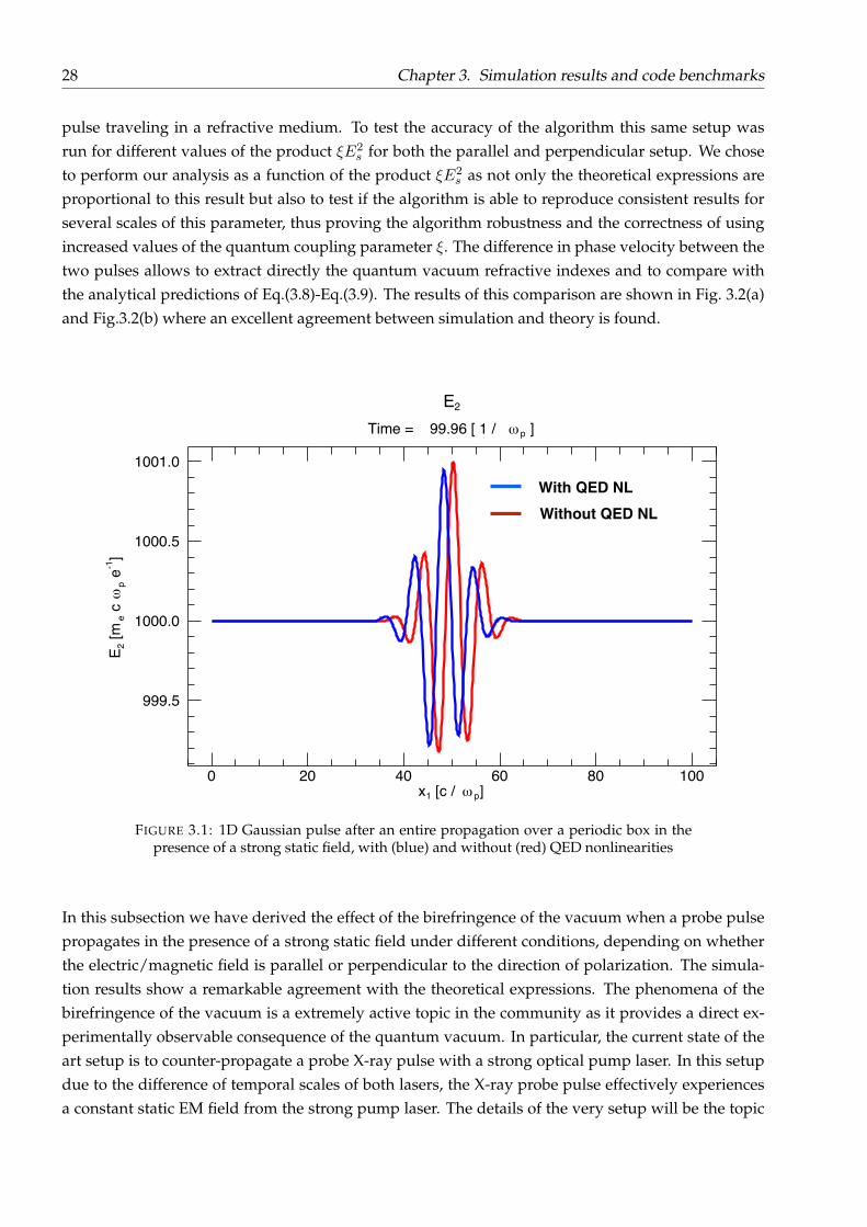
28 Chapter 3. Simulation results and code benchmarks
pulse traveling in a refractive medium. To test the accuracy of the algorithm this same setup wasrun for different values of the product ξE2
s for both the parallel and perpendicular setup. We choseto perform our analysis as a function of the product ξE2
s as not only the theoretical expressions areproportional to this result but also to test if the algorithm is able to reproduce consistent results forseveral scales of this parameter, thus proving the algorithm robustness and the correctness of usingincreased values of the quantum coupling parameter ξ. The difference in phase velocity between thetwo pulses allows to extract directly the quantum vacuum refractive indexes and to compare withthe analytical predictions of Eq.(3.8)-Eq.(3.9). The results of this comparison are shown in Fig. 3.2(a)and Fig.3.2(b) where an excellent agreement between simulation and theory is found.
E 2 [m
e c ω
p e-1
]
1001.0
1000.5
1000.0
999.5
x1 [c / ω p]100806040200
Time = 99.96 [ 1 / ω p ]
E2
With QED NLWithout QED NL
FIGURE 3.1: 1D Gaussian pulse after an entire propagation over a periodic box in thepresence of a strong static field, with (blue) and without (red) QED nonlinearities
In this subsection we have derived the effect of the birefringence of the vacuum when a probe pulsepropagates in the presence of a strong static field under different conditions, depending on whetherthe electric/magnetic field is parallel or perpendicular to the direction of polarization. The simula-tion results show a remarkable agreement with the theoretical expressions. The phenomena of thebirefringence of the vacuum is a extremely active topic in the community as it provides a direct ex-perimentally observable consequence of the quantum vacuum. In particular, the current state of theart setup is to counter-propagate a probe X-ray pulse with a strong optical pump laser. In this setupdue to the difference of temporal scales of both lasers, the X-ray probe pulse effectively experiencesa constant static EM field from the strong pump laser. The details of the very setup will be the topic

3.1. 1D Results 29
10−5 10−4 10−3 10−20.96
0.965
0.97
0.975
0.98
0.985
0.99
0.995
1
1.005
ξ Es2
n ||−1
Theory
Simulation
(a)
10−5 10−4 10−3 10−20.93
0.94
0.95
0.96
0.97
0.98
0.99
1
1.01
ξ Es2
n ⊥−1
Theory
Simulation
(b)
FIGURE 3.2: (a) Phase velocity (c = 1) of probe pulse with polarization parallel to Es,(b) Phase velocity (c = 1) of probe pulse with polarization perpendicular to Es, both as
a function of ξE2s parameter
of 4.
3.1.2 Counter-propagating plane waves
The birefringence of the vacuum discussed in the previous section is useful to explore the analyticaltechnique of solving the HE QED corrected Maxwell’s equations in a limit where one of the fields isstatic. Another limit is when two waves with similar or equal wavelength and frequency counter-propagate. This setup requires a finer mathematical treatment as there is no longer a separation ofscales that allows one to perform an ordering of the problem. Nevertheless, the procedure we willnow perform is a valuable technique to solve a set of nonlinear Maxwell’s equations with the ansatzthat the self-consistent solution is a perturbation to a well known solution of a simpler linear situa-tion. The setup consists of a 1D periodic box with two counter-propagating plane waves polarizedin the y direction, with the same frequency and amplitude, we can test how this interaction, whichwould normally result in a standing wave, is modified in the presence of the HE nonlinearities. Thisexample also serves as an ideal benchmark for the accuracy and stability of the code, once an exactanalytic result is obtained.
The theoretical analysis to address this scenario is similar to a Born series of partial waves. As-suming that the solution of the QED Maxwell’s equations are of the type
E = E(0) + E(1) + E(2) + ... (3.12)
B = B(0) +B(1) +B(2) + ... , (3.13)
where E(0) and B(0) are the unperturbed standing wave fields with frequency and wave-number,ω0 = k0 = 1, given by E(0) = E0 [cos(x− t) + cos(x+ t)] and B(0) = B0 [cos(x+ t)− cos(x− t)]whilst the remaining terms are successively higher order corrections to the standing wave fields,

30 Chapter 3. Simulation results and code benchmarks
weighted by an expansion parameter to be identified. Starting from the modified Maxwell’s equa-tions and inserting eq.(3.12) and eq.(3.13) as the expressions for the fields, we arrive at the waveequation for the first order correction to the electric field E(1)
� E1 = S1(x, t), (3.14)
where � = ∂µ∂µ, with µ = 0, 1, 2, 3, is the d’Alembert operator and the source term S1 = −∂t∂xM +
∂2t P . Inserting the zero order field in the source term, i.e. P,M = f(E(0), B(0)), we arrive at
S(1)(x, t) = 16ξE30 cos(t) cos(x) [3 cos(2t)− cos(2x)] (3.15)
This source term only accounts for the unperturbed fields being inserted into the nonlinear polariza-tion and magnetization. The formal solution of this equation is given by the convolution between thesource term and the Green’s function of the one dimensional wave operator [42],
E(1)(x, t) =
∫ L
0
∫ t
0dt′dx′G(x, x′, t, t′)S(x′, t′), (3.16)
where the Green’s function is
G(x, x′, t, t′) =1
2H[(t− t′)− |x− x′|
]. (3.17)
The modified electric field reads
E(1)(x, t) = −2ξE30 sin(t) cos(x) [2 sin(2t) (cos(2x)− 2)− 4t] . (3.18)
The corrected field exhibits a secular growth term modulated by an oscillating term. We also noticethat the relative amplitude between this term and the unperturbed field amplitude is ξE2
0 showingagain that this perturbative treatment is valid as long as ξE2
0 � 1. Taking the spatial Fourier trans-form of E(1), we verify that the fundamental mode k = k0 is reinforced by the linearly growing termand the appearance of an harmonic at k = 3k0. Defining the Fourier transform of E(x, t) as E(k, t),we obtain
E(1)(k = k0) = 4ξE30t sin(t) + 3ξE3
0 sin(t) sin(2t), (3.19)
E(1)(k = 3k0) = −ξE30 sin(t) sin(2t). (3.20)
The next order correction to the fieldE(2), reveals a k = k0 harmonic growing as t2, a secular k0 = 3k0
term and an oscillating k = 5k0 term. Repeating this process to higher orders, we can show thatthis nonlinear interaction generates odd higher harmonics from vacuum with the relative amplitudebetween these harmonics obeying the ordering
E(k = 2n+ 1) = (ξE20)nE(k = k0) (3.21)
These predictions were compared with the results of the QED solver using field amplitude of E0 =
0.0025Sch, λ0 = 1 µm plane waves and ξ = 10−9, such that the higher harmonics can be accurately

3.1. 1D Results 31
resolved above the numerical noise. The spatial Fourier transform of the fields at a certain time isshown in Fig. 3.3 for two simulations, with and without the self-consistent inclusion of HE correc-tions. We observe that when the nonlinearities are present, the odd higher harmonics are generatedwith a relative amplitude that matches the ordering given in eq.(3.21). In order to compare the sim-ulation results with eqs.(3.19-3.20), we subtracted from the full solution the classical vacuum electricfield (E0) in order to remove the zeroth order standing wave contribution. We then performed theFourier transform of this subtracted field. Finally, we tracked the temporal evolution of the ampli-tude of the k = k0 mode in Fourier space and compared it with eq.(3.19). Figure 3.4 shows thetemporal evolution of E1(k = k0) and compares the theoretical points (red) to the simulation results(blue).
|FFT
(E2)|
[me c
ωp e
-1]
102
100
10-2
10-4
10-6
10-8
k(x1) [1/(c / ω p)]86420
Time = 18.36 [ 1 / ω p ]|FFT (E 2)|
Simulation ResultsWithout QED NL
~𝛏E02
FIGURE 3.3: Spatial Fourier transform of electric field with and without QED NLpresent. The generation of odd higher harmonics can be observed in blue.
The simulation show an excellent agreement with the theoretical predictions for many laser cycles,ensuring that the algorithm is robust. Despite the one dimensionality of this example, the setup ofcounter-propagating beams is of great interest for planned experiments at extreme high intensitylaser facilities, as outlined in [29].

32 Chapter 3. Simulation results and code benchmarks
Time [1/ω0]0 10 20 30 40 50 60 70 80 90 100
E1 (k=1
) [m
Ec ω
0 e-1
]
0
0.005
0.01
0.015
0.02
0.025
0.03
0.035
0.04
Simulation results
Theoretical points
FIGURE 3.4: Temporal evolution of k = k0 Fourier mode of the subtracted electric field.
3.1.3 1D Birefringence revisited: Green function formalism
In the previous sub-section the formalism of the Green function was introduced as a mean to solve theone-dimensional wave equation with a source term. It is valuable to understand how how differentEM theoretical techniques are consistent with each other in the correct limits. In order to illustratethis we will reproduce the result of the birefringence of the vacuum derived in section 3.1.1, usingthe Green function formalism applied to the respective wave equation. Considering the field setupof a probe pulse in the presence of a strong static field in the following manner,
Ey = Ep(x, t) + Es , (3.22)
Bz = Bp(x, t). (3.23)
As in section 3.1.2 we insert the ansatz that the probe field can be decomposed inEp(x, t) = Ep0 +Ep1
where Ep0 = E0 cos(k0x − ω0t) is the unperturbed field obeying the dispersion relation ω0 = k0,φ = k0x − ω0t and Ep1 is the first order correction due to the quantum vacuum, to the unperturbedfield, which we shall now calculate. A corresponding ansatz is also valid for the magnetic field.Inserting this into the equations QED correcte Maxwell’s equations we obtain the following waveequation,
�(Ep0 + Ep1) = (∂2t − ∂2
x)(Ep1) = 4k20ξE
2sE0 cos(φ). (3.24)
this first step is exact since by construction, the wave equation differential operator applied to Ep0 iszero. The wave equation we are left with was solved by a convolution between the source term andthe appropriate Green function. This yields the following electric field,
Ep(x, t) = Ep0 + Ep1 = E0 cos(φ) + 2E0ξE2s (k0t sin(φ) + sin(ω0t) sin(k0x)) (3.25)
Eq.(3.25) contains the sum of the zero order unperturbed classical vacuum field with two correctiveterms of order ξE2
s , one with a secular growth rate and an oscillatory term. In this form, the solution

3.1. 1D Results 33
computed does not seem to be consistent with the expected result which is that the phase velocityof the probe pulse is modified. To convince ourselves that in fact this result is consistent with therefractive index Eq.(3.8) we start from the expression that is the solution of the birefringence of thevacuum and carry an expansion. We know that in a birefringent medium a wave will propagateaccording to
Ebir = E0 cos(k0x− ωt). (3.26)
Where the dispersion relation relating ω and k0 is not that of the classical vacuum, but rather ω =
vφk0 = (1 − 2ξE2s )k0. This dispersion relation was calculated using as the phase velocity consistent
with the refractive index in Eq.(3.8). To complete this derivation we will now insert this dispersionrelation in Eq.(3.26) and expand the result using a standard trigonometric identity.
Ebir = E0 cos(k0x− ωt) = E0 cos(k0x− k0(1− 2ξE2s )t) = E0 cos(φ− δωt), (3.27)
where δω = 2ξk0E2s and such that δω � ω0. This last result can be decomposed into a sum yielding
Ebir = E0 cos(φ− δωt) = cos(φ) cos(δωt) + sin(φ) sin(δωt) ≈ cos(φ) + δωt sin(φ), (3.28)
keeping a first order term in δω only. Finally, re-inserting δω, the perturbation to the frequency ofthe wave due to the quantum vacuum, yields an expression consistent with eq.(3.25), except for atransient term that becomes negligible when t� ω−1
0 . We finally obtain,
Ebir = cos(φ) + 2ξE2sk0t sin(φ). (3.29)
Compared to the previously obtained solution
EGreen = E0 cos(φ) + 2E0ξE2s (k0t sin(φ) + sin(ω0t) sin(k0x)) = Ebir + 2E0ξE
2s sin(ω0t) sin(k0x) (3.30)
This proves that solving the system of nonlinear QED corrected Maxwell’s equations via a directlinearization or using the Green’s function formalism, yields the same result.
As a discussion for future analytical techniques to be used in more complex setups, it is worthinvestigating the limitations of both techniques. Both eq.(3.29) and eq.(3.30) have an amplitude thatvaries with time whilst the wave is travelling through the birefringent medium. This variation ofamplitude does not occur in the original solution eq.(3.26). Instead, the solution in eq.(3.26) wasderived assuming that the probe pulse was already in the birefringent medium at t = 0, meaningthat there should be no change in amplitude throughout the propagation.
The changes in amplitude observed in eqs.(3.29-3.30) come from the fact that they are a limitderived from an expansion up to a certain order and valid only for short times where δωt is muchsmaller compared to unity. Therefore, we were to keep higher order terms in δω, leads to the sameresult as doing the full recursive Green function at all orders, that would not include a change inamplitude. This obsrvation leads us to conclude that rather than a change in amplitude, the termspropotional to time are a manifestation of a change in phase, but only up to a certain order.
Despite the limitations in terms of the field amplitudes presented in the approximate solutions,the phase velocity predicted in both models is identical and consistent with the simulation results

34 Chapter 3. Simulation results and code benchmarks
shown in fig.(3.2).As we shall see in Chapter 4 both phase velocity and amplitude effects in the birefringence of the
quantum vacuum have a different affect in the outcome of relevant observables in an experimentalsituation. This is an important connection that one must bear in mind when attempting to perform atheoretical analysis of more complex scenarios involving the birefringence of the vacuum.
3.2 2D Results
The one dimensional scenarios addressed in the previous sections were crucial to establish the ac-curacy and usefulness of the algorithm developed in one-dimension but also to explain analyticaltechniques one disposes of in order to tackle these problems from a theoretical point of view. How-ever, for practical purposes, the scenarios presented are limited as not only do they deal with planewaves and homogeneous static fields, but most importantly, they are oblivious to important two-dimensional finite-size beam effects that occur in real beams and laser pulses. Therefore, the gener-alization of the algorithm proposed to two-dimensions provides a tool that can be extremely com-petitive in simulating realistic scenarios with experimental relevance. This section begins with thedemonstration of the birefringence of vacuum in the presence of a static field, in two dimensions, toprove that the generalization of the algorithm to multi-dimensions does not jeopardize its accuracy.The remainder of the section is dedicated to presenting simulation results of the collision betweentwo Gaussian pulses, in different conditions, and the subsequent generation of higher harmonics.These simulations illustrate the usefulness of a multi-dimensional code in scenarios where a self-consistent analytical treatment is not available. This final feature emphasizes the usefulness of thealgorithm developed in this thesis.
3.2.1 2D vacuum birefringence
When performing a generalization from one dimension to multi-dimensions, a useful benchmarkis to verify that the one dimensional results, in a well studied scenario, can be recovered within atwo dimensional framework. Using this as motivation, a simple setup is to verify that a 2D planewave propagating in the x direction, will propagate with a phase velocity given by Eqs.(3.8-3.9) de-pending on whether the pulse is polarized parallel or perpendicular to the direction of the static field.
Figure 3.5 shows the simulation results of the phase velocity extracted from the simulation fora plane wave propagating in the x1 direction, in a 2D scenario, in the presence of a static fieldEs = 1000. The fact that the simulation results agree extremely well with the theoretical expres-sion derived for a one-dimensional pulse proves that the 2D generalization of the code is accurate inthe one dimensional limit of the birefringence of the quantum vacuum.
This test allows us to move on onto more complex simulation scenarios where a full self-consistentanalysis is not possible, with the confidence that the two dimensional code recovers the correct re-sults in the appropriate limits. In order to go beyond simulation setups using plane waves and reallyexplore the effect and complexity of finite size effects, we will now investigate scenarios using realis-tic laser pulses. In the following cases, the laser pulses used are self-consistently initialised and will

3.2. 2D Results 35
●
●● ●
●●
●
Theory, eq(3.8)
● Simulation Points
10-5 10-4 0.001 0.010 0.100
0.875
0.900
0.925
0.950
0.975
1.000
ξE02
Phasevelocity
[c]
FIGURE 3.5: Simulation results of the phase velocity of a plane wave propagating in thex1 direction in the presence of a strong static field, for different values of the quantum
parameter ξ. The corresponding prediction previously derived is plotted in red.
have an intensity varying with the distance from the axis of propagation and exhibit the focusing andde-focusing effects associated to realistic laser pulses. A revision of these effects can be found in anystandard optics textbook [43].
3.2.2 Counter-propagation of Gaussian laser pulses
In order to illustrate the usefulness of our algorithm in multi-dimensions, two setups were investi-gated in 2D: the counter propagation of two Gaussian pulses interacting at the focal point, and theperpendicular interaction of two Gaussian pulses focused at the same point. For these setups, a con-sistent analytical treatment becomes cumbersome especially due to the self-consistent treatment ofboth the transverse and longitudinal component of the pulses.
A quantum parameter of ξ = 10−6 was used for the sake of providing illustrative examples. Inthe first setup two λ = 1 µm laser beams with a normalized vector potential a0 = 50 (∼ 10−4Es innormalized units) and duration of 25 femtoseconds were counter-propagated and interacted in thepresence of the QED nonlinearities. Both beams had a waist W0 = 2.3 µm. Figure 3.6 shows thetransverse electric field of the laser beams before interaction, Fig.3.7-(a) the spatial Fourier transformof the beams with ξ = 0 (classical limit) and in Fig. 3.7-(b) the Fourier transform of the electric fieldafter the interaction (asymptotic state) including the HE corrections. As shown in Fig. 3.7-(b), afterthe interaction, odd higher harmonics are also generated as in the 1D case, with relative amplitudesconsistent with eq.(3.21). However, in this case the harmonics generated have the same Gaussianbehavior as the unperturbed pulses and attain a greater spread in Fourier space after the interaction.After the pulses have spatially overlapped, the harmonics propagate and leave an imprint of thenonlinear interaction, that co-propagates with the original beam.

36 Chapter 3. Simulation results and code benchmarks
x2 [c / ω
p]
200
150
100
50
0
x1 [c / ω p]300250200150100500
Time = 0.00 [ 1 / ω p ]
E2
E2 [m
e c
ωp e
-1]
40
20
0
-20
-40
FIGURE 3.6: Initial setup of Gaussian pulses. Both pulses are polarized in the x2 direc-tion and will focus in the center of the box.
4
2
0
-2
-4k(x1) [1/( ω 0/c)]
420-2-4
k(x 2
) [(ω
0/c)]
4
2
0
-2
-4
(a) tω0 = 160 (b) tω0 = 160
k(x1) [1/( ω 0/c)]420-2-4
|FFT
(E2)|
[me c
ω0 e
-1]
100
10-2
10-4
10-6
10-8
|FFT (E 2)|
FIGURE 3.7: Spatial Fourier transform of the electric field, (a) after the interaction butwhen QED corrections are absent, (b) after the interaction with self-consistent inclusionof the quantum corrections. k = 3k0 harmonics and small distortion of k = k0 can be
observed.

3.2. 2D Results 37
x 2 [c
/ ω
0]300
250
200
150
100
50
0x1 [c / ω 0]
300250200150100500
Time = 0.00 [ 1 / ω 0 ]
(E1,E2)
(E1,E
2) [m
e c ω
0 e-1]
40
30
20
10
0
FIGURE 3.8: Electric field setup for two Gaussian pulsed traveling in perpendiculardirections but focusing on the same point.
The second setup shown in Fig. 3.8 contains richer physics: it comprises of two 1µm Gaussianpulses with a0 = 50 and wave-numbers k1 and k2 that interact at their focus, with k1 ⊥ k2. Thebeam parameters are equal to those of the previous setup. The initial Fourier space of the beampropagating in the x direction is shown in Fig. 3.9-(a) and this spectrum would remain unalteredduring the interaction in the classical limit (ξ= 0). During the peak of the nonlinear interaction (atthe focal point) we see in Fig. 3.9-(b) that many pairs of (k1,k2) harmonic combinations are beinggenerated. More interestingly, there appears to be a continuous filling of Fourier space in betweenthe expected harmonics integer combination as the spatial overlap creates a multitude of nonlinearGaussian modes. This effect is lessened after the interaction since there is no longer a source to feedthese regions of Fourier space and only the integer expected combination of (k1,k2) harmonics areleft as an imprint of the interaction, see Fig. 3.9-(c). The longitudinal field component, inherent toa non-plane wave propagation, triggers a self-interaction of the Gaussian pulse through the QEDnonlinearities [44]. This self-interaction plays the role of a coupling source when both pulses inter-act spatially. Such terms are responsible for the (k0, 2k0) and the higher order (2.5k0, 2k0) harmonicpoints in Fig. 3.9-(b). The self-interaction coupling combined with the different propagation direc-tions, is the reason why this second setup generates several new harmonic couplings, compared with

38 Chapter 3. Simulation results and code benchmarksk(
x 2) [
1/(c
/ ω
0)]
6
4
2
0
-2
-4
-6
|FFT (E 2)|
|FFT
(E2)|
[me c
ω0 e
-1]
100
10-1
10-2
10-3
10-4
10-5
10-6
10-7
6
4
2
0
-2
-4
-6
k(x 2
) [1/
(c /
ω 0)]
6
4
2
0
-2
-4
-6k(x1) [1/(c / ω 0)]
6420-2-4-6
a) tω0 = 0 b) tω0 = 76
c) tω0 = 160
k(x1) [1/(c / ω 0)]6420-2-4-6
k(x1) [1/(c / ω 0)]6420-2-4-6
|FFT
(E2)|
[me c
ω0 e
-1]
100
10-1
10-2
10-3
10-4
10-5
10-6
10-7
FIGURE 3.9: Spatial Fourier transform for E2 field at different stages of interaction. (a)Initial Fourier space, if there were no vacuum nonlinearities this spectrum would re-main unchanged throughout the interaction. (b) At peak of nonlinear interaction whenthe pulses are completely overlapped in space. (c) Asymptotic state: after the nonlinearinteraction the pulses propagate independently but with higher harmonics generated
from the interaction.
the previous counter-propagating setup.The Fourier spectra obtained in these two setups show that the harmonics generated in either
case are distinct, thus allowing to clearly distinguish both cases. Future work will include the analyt-ical study of the relative intensity and spectral width of the generated harmonics and their possiblerelation with other beam parameters and with the fundamental interaction parameter ξ. Namely, itis of great interest to understand how the production of these higher harmonics from vacuum maybe optimized in terms of the duration of the pulses as these results can provide signatures of exper-imental relevance. A future setup to explore will also include the interaction of two laser beams atan arbitrary angle 0 < θ < π
2 radians in order to model realistic experimental conditions. If this an-gular dependence of the interaction is well understood, one could in principle determine how well

3.2. 2D Results 39
aligned two ultra-intense beams are by looking at the Fourier spectrum after a vacuum interaction.Finally, if one assumes that the parameter ξ is a well measured quantity, one could precisely mea-sure the initial intensity of the beams. This final property enhances the interest in this analysis in atime where ultra-intense laser facilities are being upgraded or constructed around the world and theexperimental techniques to measure such intensities is still not firmly established.


41
Chapter 4
Realistic scenarios of vacuumbirefringence
In chapter 3 we discussed how the HE QED corrections to Maxwell’s equations can induce the phe-nomenon of vacuum birefringence by creating an effective refractive index, greater than unity, fora pulse traveling in the presence of a strong static field. This physical consequence opens the doorto the experimental detection of the existence of the quantum vacuum, in the strong field regime.In this chapter we start by explaining the experimental setup proposed for the measurement of vac-uum birefringence followed by an extension of the theoretical analysis performed in chapter 3. Weshow that the physical observables in realistic setups are the ellipticity and angle of rotation in thepolarization of a probe pulse. We will further show how the simulations that can be performedusing the new numerical solver developed in this thesis, whilst emphasizing the fact that such isonly possible using high performance computing tools. The diagnostics created for this setup willbe explained and the results of two-dimensional simulations presented. The aim of this chapter isto prove that our work can be a valuable tool within the community to simulate currently plannedexperimental setups, without approximations, thus complementing the extensive theoretical work al-ready performed within a QED formalism. Finally, the fact that our algorithm is fully EM means thatthe results of our simulations are the fields and therefore contain information about experimentallyrelevant quantities such as phase and amplitude.
4.1 Setup and theoretical framework
4.1.1 Vacuum Birefringence: probing the quantum vacuum
As originally proposed in [38, 39] and re-examined in detail in [25, 45, 46], an X-ray probe pulse ofwavelength λX will experience vacuum birefringence when counter-propagated with a strong opticalpump laser of wavelength λ0. In particular, due to the difference of scales (λX � λ0), the X-ray probewill effectively experience a quasi-static field according to the pump profile. The setup of interest isillustrated in fig.4.1 where we see the X-ray probe pulse initially polarized at 45o compared to thepolarization of the pump pulse, leaving the region of interaction with an ellipticity induced in its po-larization as well as a rotation on the plane of polarization, due to the quantum vacuum interaction.

42 Chapter 4. Realistic scenarios of vacuum birefringence
Input x-ray probe
Optical Pump
Output x-ray probe
FIGURE 4.1: Experimental setup proposed to study the birefringence of the quantumvacuum via the change in the ellipticity of the polarization of a X-ray probe pulse, after
trasversing a strong optical pump laser.
This setup was first proposed in [39] including a theoretical analysis that did not take into accountthe fact that the pump laser has a profile which varies with space and time. Since then, more pow-erful theoretical methods have been employed to predict the rotation of polarization and ellipticitythat is expected to be observed for more complex setups taking into account finite-size beam effects.In particular, in [45] the authors use a QED M-matrix scattering formalism in order to compute thenumber of probe photons that flip between the two possible polarization states as well as the mo-mentum distribution of the scattering photons, thus predicting how the probe will be modified afterthe interaction whilst taking into account the approximate beam structure of the pump. The authorsof [46, 47] use a so-called light-front QED formalism, whereby they integrate over the world-line of agiven photon within the probe pulse, in the presence of the background EM field created by the opti-cal pump. Despite the impressive results derived in the works described, approximations regardingthe pump and probe profiles must be made within both theories. These include neglecting the longi-tudinal component of a Gaussian beam, or limitations due to the paraxial approximation. We wouldlike to emphasize that since our code solves the exact set of nonlinear Maxwell’s equations for anarbitrary field configuration, we are able to go beyond such approximations and deliver exact resultswithin the precision of the numerical scheme. Having explained the state of the art regarding the the-oretical methods to tackle this problem, we will describe in the next section, from an electromagneticpoint of view, why the phenomena of rotation of polarization and induced ellipticity occur.
4.1.2 Birefringence in a static field revisited
We will start with a one-dimensional approach to the problem and successively increase the com-plexity of the setup whilst bench-marking our results with the code. Consider a one-dimensionalpulse propagating in a background static electric field, as already addressed in section 3.1.1, with apolarization at an arbitrary angle to direction of the static electric field. Without loss of generality, the

4.1. Setup and theoretical framework 43
field setup can be written as
Ey = Es + cos(θ)Ep , (4.1)
Ez = sin(θ)Ep , (4.2)
By = − sin(θ)Ep , (4.3)
Bz = cos(θ)Ep , (4.4)
withEp = Ep0 cos(k0x− ωt) exp(−(x− x0 − ct)2/2σ2),
as the expression for the probe pulse package of frequency ω, wave-number k0, σ the duration ofthe pulse, Ep0 the amplitude and x0 defining the initial position. Furthermore, Es represents thestrong static field and θ the arbitrary angle between the direction of Es and the polarization of theprobe pulse. As we have seen in sec.3.1.1, the static electric field will induce a non-unity refractiveindex of the vacuum making the probe pulse travel with a phase velocity different from c. We alsoshowed that the refractive index of the vacuum depended on the direction of the polarization of theprobe pulse relative to the direction of the static field. In this scenario, the polarization of the probepulse can be decomposed parallel and perpendicular components relative to the direction of thestatic field, such that each one of these field components will experience a different refractive indexgiven by Eqs.(3.8-3.9) respectively. This setup is analogous to a bi-axial homogeneous anisotropicmedium, defined such that the electric permittivity and magnetic permeability tensors are diagonalmatrices whose elements in general differ. The fact that each field component will travel with adifferent phase velocity means that they continuously dephase from each other as they propagate inthe quantum vacuum. The relative phase between both components introduced by the propagationis called retardance. The retardance introduced in this case is very small since the corrections to therefractive index of the vacuum are of the order ξE2
s . Nevertheless, this retardance will induce a smallellipticity in the polarization of the probe pulse, as we shall now prove. The approximate phasevelocity for the parallel and perpendicular field components are given by the inverse of the refractiveindexes as,
v‖ = 1− 2ξE2s , (4.5)
v⊥ = 1− 7
2ξE2
s . (4.6)
Assuming that the polarization angle is θ = π4 , we obtain the following expressions for the fields:
~Ep(t, x) =A(x)√
2
(exp(−jωt) exp(jk‖x)~ey + exp(−jωt) exp(jk⊥x)~ez
), (4.7)
where A(x) is the spatial pulse envelope with a Gaussian profile and k‖, k⊥ denote the parallel andperpendicular wave-numbers respectively. After a propagation time T over a distance d and usingthe relation between vφ and the wave-number, we can re-write the above expression making it clear

44 Chapter 4. Realistic scenarios of vacuum birefringence
the ellipticity induced in the polarization is due to the retardation effect,
~Ep(T, d) =A(x)√
2
[exp(−jωT ) exp(jk‖d)~ey + exp(−jωT ) exp(jk⊥d)~ez
](4.8)
=A(x)√
2exp(−jωT )
[exp(jk0(1− 2ξE2
s )d)~ey + exp(jk0(1− 7
2ξE2
s )d)~ez
](4.9)
=A(x)√
2exp(−jωT ) exp(jk0d) [exp(−jδ)~ey + ~ez] exp(−jk0
7
2ξE2
sd), (4.10)
where δ = (72 − 2)ξE2
sk0d = 32ξE
2sk0d is the difference of phase between both the field components
and is defined as the ellipticity induced on the probe pulse due to the quantum vacuum interaction. Itmust emphasized at this point that an ellipticity in the polarization of a pulse is a directly observablequantity thus representing an experimental signature of the nonlinear quantum interaction betweenthe probe field and the background static field. In particular, techniques to measure extremely smallellipticities of the order of 10−9 for x-rays and 10−6 for optical lasers, have been developed in recentyears [48]. To conclude this section we reiterate that the ellipticity induced in the polarization of apulse traveling in the presence of a static electric field is approximately
δ =3
2ξE2
sk0d =3
2
2πd
λ0ξE2
s . (4.11)
The fact that this result is proportional to the ratio d/λ0, is physically relevant as it means that thegreater the interaction length (d) compared to the vacuum wavelength λ0, the greater the ellipticityinduced. This model is however over-simplistic as in realistic scenarios, the role of the backgroundstrong static field is replaced with that of an ultra-intense laser pulse with optical frequency suchthat from the point of view of the probe pulse (x-ray), the field is effectively static over long periodsof interaction. As is clear from the simulations performed in Chapter 3, the setup described in thissub-section is straightforward to simulate in order to verify how accurate eq.(4.11). However, beforethis is done, we will briefly digress to address the issue of how the ellipticity of the polarization maybe extracted from the simulation in a systematic and reliable way.
4.1.3 Post-processing diagnostic: polarization diagnostic
In the study of the birefringence of the vacuum with the aim of simulating experimentally relevantEM setups, it is imperative to use a diagnostic able to measure the polarization of a laser pulse. Ingeneral, due to the dynamic nature of the quantum vacuum interactions, the polarization of a pulsemay be varying in space during different time intervals of the simulation box. Therefore, we devel-oped a diagnostic that acts as a polarization detector that can be placed, for specific time intervals,in a given spatial position of the simulation. To illustrate the use of this diagnostic, consider the one-dimensional setup shown in fig.4.2(a). In this example,the detector is placed at the position x1 = 150
and the probe pulse travels through a static background electric field. The detector we developedwill record pairs of field values (Ez, Ey) at that point, as a function of time. Each of these points willthen be plotted in a (Ez, Ey) graph, thus allowing us to visualize the relative phase between bothfield components in time and measure the polarization of the pulse. This result is shown in fig.4.2(b).As this figure shows, we see a straight line of gradient one, confirming that the pulse is polarised

4.1. Setup and theoretical framework 45
with an angle θ = −π/4 in the y − z plane. However in fig.4.2(b) it can also be seen that the linehas a small thickness. This thickness is due to the fact that the polarisation has now the form of anextremely oblate ellipse. As the ellipticity induced cannot easily be resolved in fig.4.2(b), we performthe following trick: since we know that the ellipse has it’s major axis coinciding with a line of gra-dient one in this graph, we rotate the coordinate system by an angle θ = −π/4 using the followingtransformation:
x′ = x cos(θ)− y sin(θ) (4.12)
y′ = y cos(θ) + x sin(θ), (4.13)
where it is readily verified that the transformation matrix has a determinant equal to one. Apply-ing the above transformation to the data collected by the detector, we obtain fig. 4.2(c) where thestructure of the ellipse can be resolved in a far clearer way. Essentially, this transformation makes thex-axis of the figure correspond with the major axis or the ellipse. Finally, the diagnostic developedperforms one final stage by fitting the data obtained to the general expression of an ellipse in thegeneral quadratic form, given by
a′x2 + 2b′xy + c′y2 + 2d′x+ 2e′y + f ′ = 0 , (4.14)
with fitting coefficients a′, b′, c′, d′, e′ and f ′. The fitted ellipse is then plotted on the same figureas the data points and the fitting coefficients converted to the more useful ellipse parameters thatparametrise an ellipse in the general form. Figure 4.2(d) shows the result of this fit in blue. Phys-ically, the magnitude of the ellipticity induced is a measure of the flatness of the ellipse which isdirectly related to the magnitude of the quantum vacuum interaction.
The diagnostic developed includes a simple graphic interface that plots the simulation domainand allows the user to select where the detector has to be placed in a dynamical way. This featurecombined with the fact that the detector is able to probe whatever time scales of the simulation de-sired, makes this a very useful and robust tool to analyse scenarios where, for example, the ellipticityinduced on the probe pulse, varies as a function of the distance.
Finally, regarding the coordinate rotation performed to center the ellipse, it is worth noting thatif after a rotation by the initial angle of polarisation (in this case θ = π/4), there remains a residualde-centering of the major axis of the ellipse compared to the new x-axis, it means that the angle ofthe rotation performed does not coincide with the polarization angle of the pulse. This residual angleshows that during the interaction a rotation in the plane of polarisation of the probe pulse occured.This is a different physical effect called rotation of the angle of polarization, which we will shortlyexplain, that can eventually be another signature of the a quantum vacuum interaction. This effectis relevant in more complex setups where the amplitude of both field components change in a non-trivial way.
To illustrate the importance of the diagnostics developed, coupled with the QED solver, we willnow use the ellipse fitting parameters obtained to extract the ellipticity of the polarization obtainedin the example above and compare it with the theoretical result, eq.(4.11). To achieve this, we must

46 Chapter 4. Realistic scenarios of vacuum birefringenceE 2
[me c
ωp e
-1]
1001.0
1000.5
1000.0
999.5
999.0
x1 [c / ω p]5004003002001000
Time = 0.20 [ 1 / ω p ]E2
Detector position
Ey-1.5 -1 -0.5 0 0.5 1 1.5
E z
-0.015
-0.01
-0.005
0
0.005
0.01
0.015
Ey-1.5 -1 -0.5 0 0.5 1 1.5
E z
-0.015
-0.01
-0.005
0
0.005
0.01
0.015
Ey-1 -0.5 0 0.5 1
E z
-1
-0.8
-0.6
-0.4
-0.2
0
0.2
0.4
0.6
0.8
1(a) (b)
(c) (d)
FIGURE 4.2: (a) Setup described in section 4.1.1 where a probe pulse polarized with anangle θ = π
4 propagates in the presence of a strong static field, Es = 1000 (b) Resultof polarization diagnostic returned by the detector showing a line of gradient one butwith a small thickness caused due to the ellipticity induced in polarization of the pulse.(c) Polarization graph of the points presented in (b), rotated by θ = −π4 as to centerthe coordinate system such that the horizontal axis coincides with the major axis of theellipse, thus resolving the ellipticity in a more precise way. (d) The diagnostic finallyperforms a fit using the least squares method of the outer points of the ellipse to the
general quadratic equation for an ellipse, eq.(4.14).
first obtain an expression that relates the geometrical parameters of an ellipse (major radius, minorradius etc.) to the physical ellipticity of the polarization. A general derivation of the relation betweenthe structure of the EM fields and the corresponding geometric parameters of the ellipse inducedin the polarization, is presented in Appendix A. For this example, we show that the ellipticity δ isdirectly related to the minor radius b of the ellipse by the expression
b =Ep√
2δ , (4.15)
where Ep is the initial amplitude of the probe pulse and δ is the ellipticity, already defined as the

4.1. Setup and theoretical framework 47
accumulated phase difference between the two components of the probe pulse. Figure 4.3 showsthe rotated ellipse and corresponding fit for the simulation performed with the setup previouslydescribed of a probe pulse propagating in the presence of a strong static field. The simulation wasperformed with a probe pulse with a 0.1 keV pulse with a normalized wave-vector k0 = 10 andamplitude Ep = 1, in the presence of a static field of normalized magnitude Es = 1000. The quantumvacuum coupling parameter used was ξ = 10−11 and the detector was placed at x = 150, suchthat the length of interaction is equivalent to d = 100. All parameters were normalized with thesame normalizations as in section 3.1.1. The fit returned a minor radius of the ellipse b = 0.0103
corresponding to an ellipticity of
δsim =
√2b
Ep= 0.0143
whereas the expected theoretical value is
δtheo =3
2ξE2
sdk0 =3
2× 10−1110002 × 100× 10 = 0.015 .
Therefore, the ellipticity extracted from the simulation is accurate compared to the theoreticalprediction. This finding not only serves as an excellent benchmark for the precision of the code, butalso proves that the diagnostic developed serves as a powerful tool to study birefringence scenarios.Finally, there is one crucial feature revealed by the simulation results in this setup that must be em-phasized. Since the strong static field is present throughout all the spatial domain of the simulation,it acts as a constant source of vacuum birefringence making the ellipticity constantly increase withthe propagation distance as the probe field components are continuously becoming more de-phased.In fig.4.3, we see that the ellipse formed is actually a spiraling ellipse whose minor radius is contin-uously increasing. This means that, if we were to place the detector at a distance d2 = d + ∆, thenthe minor radius, and corresponding ellipticity induced would also increase by the ratio d2/d. Thiswill not be the case in more sophisticated setups where the x-ray probe pulse will interact with anoptical pump laser, due to the finite length of the interaction created by the profile of the pump. Thisexample also serves to illustrate a feature that is intuitive from the start: the greater the interactionregion of the quantum vacuum is, the greater the induced ellipticity. Thus, we should place a strongoptical laser as a pump, ideally, as intense as possible, for the longest duration possible. Finally, animportant consequence that emerges from this analysis is that the ellipticity induced in the probepulse due to vacuum birefringence is a cumulative effect.
We have shown, via simulations, that for a pulse propagating with a linear polarization of angle0 < θ < π/2 relative to a strong static field, there is an ellipticity induced in the polarization dueto the quantum interaction of vacuum birefringence. We developed a simple theoretical model toexplain the ellipticity induced and predict it’s value. We then compared the theoretical value calcu-lated to that extracted from the simulation results using a diagnostic we developed. This comparisonyielded an extremely accurate result thus proving the how powerful the algorithm developed in thisthesis can be deliver simulation results showing a variety of phenomena associated to the quantumvacuum. With the tools developed so far and motivated by accurate results in the example presented,in the next sections we will tackle more realistic setups, from both a theoretical and simulation point

48 Chapter 4. Realistic scenarios of vacuum birefringence
Ey-1.5 -1 -0.5 0 0.5 1 1.5
E z
-0.015
-0.01
-0.005
0
0.005
0.01
0.015
b
a
FIGURE 4.3: Polarization plot showing the ellipticity induced in the polarization of theprobe pulse after propagating in a birefringent vacuum, caused by a strong static field,over a propagation distance d = 100. The labels a and b define the major and minorradii of the fitted ellipse respectively and are an output of the diagnostic developed.Using these values we can extract the value of the ellipticity induced in the polarisation
of the pulse, from the simulation.
of view. The ultimate aim being to provide realistic predictions for quantum vacuum signatures thatcan be expected in planned experimental scenarios.
4.2 2D Birefringence with a realistic pump profile
In the previous section we studied the ellipticity induced in the polarisation of a probe pulse propa-gating in the presence of a strong static field. Despite providing useful physical insight, this scenariodoes not accurately portray a realistc experimental scenario where it is a strong optical laser pump,whose profile is not static, that creates the birefringence of the vacuum for the X-ray pulse. To addressthis, we simulate the following 2D setup, in a 1D limit, illustrated in fig.4.4, where a 10 keV X-ray iscounter-propagated with a 1 µm optical pulse, both with duration of 40 fs. The intensity of the opticalpump is 1023 Wcm−2 whereas the X-ray laser had an intensity of 1018Wcm−3. These parameters were

4.2. 2D Birefringence with a realistic pump profile 49
chosen according to the proposed beam parameters for the LCLSII update and the new SLAC X-raylaser. As shown in fig. 4.4(a), the transverse profile of the lasers was chosen to be constant (planewave in 2D). This was done so that we can gradually increase the complexity of the setup and beginby studying exclusively how introducing a profile to the pump laser effects the ellipticity induced,rather than including at this stage the greater complexity of transverse beam effects.
x 2 [c
/ ω
p]
10
8
6
4
2
0x1 [c / ω p]
80006000400020000
Time = 0.00 [ 1 / ω p ]
|E 2|
|E2|
[me c
ωp e
-1]
1.0000
0.1000
0.0100
0.0010
0.0001
x-ray probe Optical pump
x-ray probe (x1000)
Optical pump
(a) (b)
Field line-out for constant x2
FIGURE 4.4: (a) 2D Contour plot of the field setup we wish to simulate. In this sim-ulation we counter-propagate a weak X-ray probe laser (traveling to the right) with astrong optical laser (traveling to the left). In the transverse direction there is no profileof the beams, making this setup in practice quasi one-dimensional. (b) line-out for aconstant x2 of the plot shown in (a) where we can see the longitudinal profile of each
laser as well as the difference in wavelengths
We will now address, from a theoretical perspective, the EM setup showed in fig.4.4. The startingpoint fo describe this scenario is given by the following field configuration
Ey =1√2Epy + E0(x, t) , (4.16)
Ez =1√2Epz , (4.17)
By = − 1√2Bpy , (4.18)
Bz =1√2Bpz −B0(x, t) . (4.19)
Where E0(x, t) = B0(x, t) represent the self-consistent fields of the optical pump envelope. Tocreate a model to tackle this scenario using an EM model, we will apply the WKB (Wentzel-Kramers-Brillouin) method to solve the wave equation for the probe pulse, taking into account the profile ofthe pump. Let us briefly explain the basis of the WKB method and explain why it can be applied toour problem.

50 Chapter 4. Realistic scenarios of vacuum birefringence
4.2.1 Solving the wave equation using the WKB approximation
Many problems in physics, once formulated,have the need to solve a wave equation. The full homo-geneous wave equation for the variable y(x, t), normalized such that vφ ≡
vφc can be written as(
∂2x −
1
v2φ
∂2t
)y(x, t) = 0, (4.20)
where vφ is the phase velocity of the wave. Applying the anstatz that y ∼ A(x)ejωt yield the wellknown 1D Helmhotz equation (
∂2x −
ω2
v2φ
)A(x) = 0 . (4.21)
Defining the wave number k = ωvφ
, eq.(4.21) can be solved for A(x) where two constants, c1 and c2
still need to be determined by the initial conditions. This solution is given by
A(x) = c1 exp(jkx) + c2 exp(−jkx) , (4.22)
where the sign of each exponential will define the direction of propagtion. This derivation is valid aslong as the wave number is constant. The WKB approximation can be used to solve wave equationsin the form of eq.(4.21) but with k being a function of the coordinate of the differential equation.Therefore we wish to solve the following wave equation,
(∂2x − k2(x)
)A(x) = 0 , (4.23)
by assuming the solution is of the form
A(x) = c3 exp
(±j∫k(x)dx
). (4.24)
To verify the validity of this solution, we insert the ansatz in eq.(4.23) and by inspection try to under-stand when the solution is valid. This calculation can be easily shown to yield,
(∂2x + k(x)2
)exp
(±j∫k(x)dx
)= ±jk′(x) exp
(±j∫k(x)dx
). (4.25)
Therefore, if the right hand side of eq.(4.25) is negligible compared to the left hand side, the ansatz isvalid. This will be the caseh as long as the scale of variation of the wave number is slow compared tothe magnitude of the wave number. This criteria can be defined more rigorously by comparing theorder of both terms in eq.(4.25), yielding
dk(x)
dx
1
k2(x)� 1 . (4.26)
It can be shown that the next order of the WKB approximation leads to a correction in the amplitudeof the wave to account for the conservation of energy flux. This leads us to state the solution of

4.2. 2D Birefringence with a realistic pump profile 51
eq.(4.23) under the WKB approximation
A(x)WKB =1√k(x)
exp(±j∫k(x)dx) . (4.27)
For the purposes of our work we must solve a wave equation for a probe pulse in the case where therefractive index of the quantum vacuum (which is closely related to the wave number), is varyingin space, during the interaction, due to the presence of the optical pump laser. As we will showwhen we derive the dispersion relation for the probe laser in the presence of the probe pulse, it isreasonable to assume a phase velocity for the probe pulse of the type
vφ = 1 + αξE20(x),
where α is a constant and E0(x) the profile of the pump laser. Applying the relation between wavenumber and phase velocity and assuming that this profile can be decomposed as a product of anamplitude with an arbitrary function of order one with a scale of variation λ0, E0(x) = E0g(x), weobtain that
k(x)2 ≈ k2p
[1 + 2αξE2
0g2(x)
], (4.28)
where kp is the wave number of the probe in the classical vacuum. Inserting this expression for thewave number in the criteria of validity eq.(4.26) derived from the original wave equation yields thecondition under which the WKB approximation can be used for our setup. This criteria is therefore,
λpλ0� 1. (4.29)
The approximation is therefore valid in the slowly varying package limit, or in other words, as longthe the wave-length of the probe pulse is much smaller than the wavelength of the probe laser. Thiscondition is readily verified in the experimental conditions of interest due to the difference of scalesof the x-ray probe pulse compared to the optical pump laser.
In this section we have derived the WKB approximation as a powerful tool to solve wave equa-tions with a spatial-dependent wave number. We then applied the WKB criteria to the setup ofinterest in the context of vacuum birefringence and showed that the method can be applied due tothe separation of scales between the two laser pulses. Finally, note that this method allows us tocalculate the total phase accumulation of the probe pulse after interacting in the quantum vacuumby simply integrating over the profile of the pump laser. This technique will be extremely useful inderiving analytic results for the retardance, and thus the ellipticity induced, in the probe pulse afterthe interaction.
4.2.2 Derivation of the dispersion relation
The WKB derivation of the previous sub-section requires a dispersion relation that specifies the spa-tial dependence of the wave-number. This will be the purpose of this sub-section, where we will

52 Chapter 4. Realistic scenarios of vacuum birefringence
show that not only is the dispersion relation far more complicated than in the case of a simple strong-static field, but also, new physical phenomena appear due to the fact that the pump fields vary inspace and time. To derive the correct dispersion relation we start by calculating the EM invariantsthat result from the field setup present in eqs.(4.16-4.19), this yields the following non-vanishinginvariants:
E2 −B2 = 2EpyE0 + 2BpzB0 ,
~E · ~B = −(E0Bpy +B0Epz).
Using these invariants it is now possible to calculate all components of the polarization and magne-tization of the quantum vacuum, neglecting terms of order E2
pE0 or smaller. This yields:
Py = 4ξ(E2
0Epy +B0E0Bpz), (4.30)
Pz = 7ξ(B2
0Epz + E0B0Bpy), (4.31)
My = −7ξ(E2
0Bpy + E0B0Epz), (4.32)
Mz = 4ξ(B2
0Bpz + E0B0Epy). (4.33)
With these expressions one must now derive the wave equation for both the electric field com-ponents, parallel and perpendicular to the polarization of the pump field. Note that in this scenarioboth the probe and the pump laser will have a corresponding wave equation that is affected by theQED nonlinearities. However, to make the calculations feasible, we assume that the pump laser isunaffected by the nonlinear interaction with the probe laser. This assumption is reasonable not onlydue to the difference in amplitudes of each field but it is also a standard assumption when derivinginstabilities in plasma physics such as Brillouin or Raman amplification. Taking these considerationsinto account, we obtain the following wave equation for the parallel component of the probe pulse,
�Epy = 4ξ(2(∂t∂xE
20 − ∂2
tE20)Epy + (∂xE
20 − 3∂tE
20)(∂tEpy − ∂xEpy) + 2E2
0∂t∂xEpy − E20(∂2
x + ∂2t )Epy
).
(4.34)This differential equation is of the form of a wave equation with a source term linear in Epy and
it’s derivatives but with nonlinear coefficients. Before arriving to the final dispersion relation we willre-write eq.(4.34) in a way that offers greater physical insight regarding what physical effects can beexpected,
(a‖∂2t − b‖∂2
x)Epy = α‖Epy + γ‖(∂tEpy − ∂xEpy) + β‖∂t∂xEpy , (4.35)
Where the coeficients are defined as
α‖ = 8ξ(∂t∂xE20 − ∂2
tE20) ,
γ‖ = 4ξ(∂xE20 − 3∂tE
20) ,
β‖ = 8ξE20 ,
a‖ = 1 + 4ξE20 ,
b‖ = 1− 4ξE20 .

4.2. 2D Birefringence with a realistic pump profile 53
An important test of this result it to verify the limit where the pump field has no spatial or tem-poral variations (case of a strong static field), we recover the wave equation where only the refractiveindex of the probe pulse is changed. In this limit we set all derivatives of the pump field to zerowhich amounts to, α‖, β‖, γ‖ → 0 which leads to the correct result.
Equation (4.35) can de solved by inserting the ansatz Epy ∼ ejk−jωt and solved for ω yielding theself-consistent dispersion relation. Note that despite the coefficients having spatial and temporal de-pendence due to the pump laser profile, they vary on a larger scale compared to the characteristicfrequency and wavelengths of the probe pulse which permits to approximate these coefficients asquasi static and apply the WKB approximation as described in section 4.2.1. Applying the ansatz weobtain the following dispersion relation,
a‖ω2 + ω(jγ‖ − β‖k)− (k2b‖ + α‖ − jγ‖k) = 0 . (4.36)
The dispersion relation is quadratic in ω and can therefore be solved using the quadratic formula toyield two roots. Before showing the final result we would like to emphasize the fact that all com-ponents proportional to γ‖ in Eq.(4.36), are purely imaginary. This imaginary component in the dis-persion relation means that the solution to Eq.(4.36) will be complex, with an imaginary componentthat will lead to an exponential growth or damping of the probe amplitude in time. Applying thequadratic formula to Eq.(4.36) yields,
ω =β‖k − jγ‖ ±
√(jγ‖ − kβ‖)2 − 4a‖(jkγ‖ − b‖k2 − α‖)
2a‖. (4.37)
From Eq.(4.37), we confirm that a imaginary component arises in the dispersion relation, fromthe first term proportional to γ‖ and also from the square-root which is a complex number. Thisexpression appears to depend on all the coefficients in a complex manner. However, taking intoaccount the orderings for realistic simulation parameters, this expression can be heavily simplified.To perform this ordering, one must simply replace the spatial and temporal derivatives of the pumppulse by the characteristic scale of variation, 1/σ where σ is the duration of the pump laser. Thisprocess finally yields the following expression for the real and imaginary parts of the dispersionrelation,
ω = ωr + jωi , (4.38)
ωr ≈ k
(√b‖
a‖−
β‖
2a‖
), (4.39)
ωi ≈γ‖
2a‖
(1 +
√a‖
b‖
). (4.40)
Equations (4.38-4.40), completely describe the propagation of the parallel component of the probepulse. The same calculation was repeated for the component of the probe perpendicular to the pump

54 Chapter 4. Realistic scenarios of vacuum birefringence
laser yielding equations exactly in the same form but with the coefficients changed to,
α⊥ = 14ξ(∂t∂xE20 − ∂2
tE20),
γ⊥ = 7ξ(∂xE20 − 3∂tE
20),
β⊥ = 14ξE20 ,
a⊥ = 1 + 7ξE20 ,
b⊥ = 1− 7ξE20 .
A crucial conclusion of this analysis is the fact that both the real part and imaginary part of the dis-persion relation for the parallel and perpendicular components are different. This means that thephase velocity of each component will be different and thus an ellipticity will be induced in the po-larisation as already discussed previously. Furthermore, we have shown that there is a dampingin the amplitude of the probe pulse due to the space-time variation of the pump laser during thenonlinear interaction. The fact that the damping factor is different for both the parallel and perpen-dicular components means that after the interaction, they will no longer have the same amplitude.This mismatch in the amplitude of both components, small as it may be, will induce a rotation in thepolarization angle of the probe pulse that will be detected when the probe pulse crosses the detector,as explained in 4.1.3. Finally, the fact that the damping rate does not depend on the probe wave-number but rather only on the characteristics of the pump, is a valuable conclusion.The phenomena of the rotation of polarisation had already been predicted in previous work [29, 46,47] by computing the number of photon that flip from one polarisation to another using a QED for-malism. Furthermore, Dipiazza et.al in[29], predicted the rotation of polarisation in a different setupusing an EM formalism. However, to our knowledge, the derivation presented here is a novelty re-garding the setup proposed, and the dispersion relation, Eqs.(4.38-4.40), had not yet been derived.
So far, in the previous sections we derived the two observable physical consequences from the quan-tum interaction between a strong optical pump laser and a X-ray probe. In particular, we showedthat the different phase shifts introduced in each polarization component of the probe due to therespective phase velocities induces an ellipticity in the polarization whilst a damping mechanism inthe amplitudes of each polarisation component yields a rotation in the direction of polarisation ofthe pulse. As already emphasized, this setup of great experimental relevance, can be simulated withthe algorithm developed in our work. In the next section we will analyse the results of the simula-tions performed and compare with our theoretical predictions in both a quantitative an qualitativemanner.
4.2.3 Simulation result analysis
A crucial feature present in the simulations performed is the difference in scales between the twolaser pulses. This difference in scales (optical to X-ray) is about 3 orders of magnitude. Furthermore,the simulation parameters had to be such that the wavelength of the X-ray probe could be resolvedwith a criteria of 20 points per wavelength but also the width of the wave packages must be captured

4.2. 2D Birefringence with a realistic pump profile 55
within the simulation domain. Finally, and the simulation duration has to be such that the time be-fore, during and after the interaction can be simulated. These restrictions bring us to a crucial pointof this work: the fact that large computational resources are necessary to perform such simulationsand that the algorithm must be fully paralelized to operate on large computing clusters.The simu-lations about to be presented were performed at the ACCELERATES cluster (Lisbon, Portugal). Atypical simulation about to be presented lasted 12 hours using 1800 cores of ACCELERATES which isequivalent to approximately 22k computational hours. The fact that the algorithm we implementedwas done so in a fully parallel way represents a significant competitive advantage.
Table ?? summarizes the laser parameters used for the simulations and corresponding real parame-ters before normalization. The laser parameters used correspond to the proposed beam parametersfor the LCLSII update and the new SLAC X-ray laser. Finally, regarding the value of the quantumcoupling parameter ξ, we chose to vary this parameter whilst maintaining the remaining simulationparameters constant. We chose to do so for several reasons, most importantly it allows us to verify ifthe physical consequences we wish to observe scale linearly with the coupling parameter, but also torule out numerical artifacts that may only occur below certain values of the ξ parameter. The latterreason is important as we must not forget that the nonlinear vacuum corrections are small comparedto the unperturbed fields and therefore, from a computer precision point of view, there will be a limitto the precision of the machine, as well as numerical noise issues.
Physical QuantityPump Laser Probe Laser
Real value Normalised Real value Normalisedω 1.88× 10¹⁵ – 9.5× 10¹⁸ –λ 1 µm 1001 1.2 nm 1
Intensity (W cm−3) 1023 – 1018 –Electric field (V/m) 8.69× 10¹⁴ 0.34 2.75× 10¹² 0.001
Duration (fs) 40 316 40 316
TABLE 4.1: Laser parameters for the LCLSII update and the new SLAC X-ray laser. Forthe simulations performed for this setup all quantities were normalised to the X-ray
frequency.
The one-dimensional theory previously presented can be applied to the simulation setup shown infig.4.4 as we used plane waves in the transverse direction for both probe and pump. However, thelongitudinal profile of both pulses can be intialised with any function desired. In particular, it is ofinterest to test how the results vary according to the wave packet of the pump laser. To understandthis dependence, we performed simulations of the setup illustrated in fig.4.4 for different values of ξparameters but also for two different functions for the pump laser profile:
E0(x, t = 0) = E0 exp
(−(x− x0)2
2σ2
), (4.41)
E0(x, t = 0) = E0 cos(k0x) exp
(−(x− x0)2
2σ2
). (4.42)

56 Chapter 4. Realistic scenarios of vacuum birefringence
Where k0 and σ are the wave-number and duration of the pulse, respectively. These profiles wereselected to compare the induced ellipticity and rotation of polarisation when the pump laser is aGaussian package to when that same package is modulated by an oscillating function. Most impor-tantly, whilst eq.(4.42) has associated to it two spatial scales (σ, k0), the profile in eq.(4.41) only hasone scale of variation. Furthermore, as we saw in section 4.2.1, the spatial integral over the square ofthe pump profile is an important quantity that measures the effective length of interaction betweenthe probe pulse and the birefringent medium. The physical reason behind this is the fact the phaseof a wave in an inhomogeneous media is the sum of the optical phase in each layer of infinitesimalwidth. This motivates us to calculate the spatial integral of the square of both pump profiles in orderto estimate what can be expected in each case. This calculation yields,∫ ∞
−∞exp
(−(x− x0)2
2σ2
)dx = E2
0
√σ2π, (4.43)∫ ∞
−∞cos2(k0x) exp
(−(x− x0)2
2σ2
)dx = E2
0
√σ2π
(e−(k0σ)2 + 1
2
). (4.44)
Eq.(4.43) can be recovered as a limit of Eq.(4.44) by taking limit k0 → 0 which corresponds exactly tomaking the wavelength of the oscilating modulation of the pump laser to infinity thus recovering thelaser profile eq.(4.41) from eq.(4.42). Furthermore, since for the simulations performed, the quantityk0σ ≈ 20, the exponential of this number squared in eq.(4.44) is approximately zero, meaning that inpractice, the results of these integrations differ approximately by a factor of two, i.e.∫ ∞
−∞exp
(−(x− x0)2
2σ2
)dx = E2
0
√σ2π, (4.45)∫ ∞
−∞cos2(k0x) exp
(−(x− x0)2
2σ2
)dx → E2
0
√σ2π
2. (4.46)
This last limit corresponds to the existence of multiple wavelengths within the pump envelope. Wetherefore expect the results of the simulations for both cases, in terms of the ellipticity induced androtation of polarisation, to differ by a factor of approximately two.
The simulations were performed for values of ξ = [10−4 − 10−7] for both profiles. Figure 4.5(a),shows the result of the ellipticity diagnostic after a rotation by θ0 = −π/4 applied to a simulationwith ξ = 10−4 and the pump profile eq.(4.41). In red, we see the plot of the fitted expression to theouter ellipse. Figure 4.5(a) shows that an ellipticity was induced and a polarisation rotation of theprobe pulse. This angle of rotation can be measured from this diagnostic by measuring the anglebetween the major axis of the ellipse and the horizontal axis in Fig. 4.5(a). This angle is automati-cally given as an output of the fitted ellipse and serves as a direct measurement of the rotation in thepolarisation. Figure 4.5(b) shows the same ellipse, but further rotated by this residual angle from therotation in polarisation thus centering the ellipse about the Ey axis. A new fit of the centered ellipsewas performed and is shown in Fig.4.5(b). This procedure was done to show that the ellipse parame-ters obtained from the fit are invariant under coordinate rotation. Finally, one qualitative conclusioncan be extracted from the result if this diagnostic: in Fig. 4.5(a) the major axis of the ellipse makes anegative angle with the horizontal axis after being rotated by the initial polarisation angle θ0 = π/4,

4.2. 2D Birefringence with a realistic pump profile 57
which means that the polarisation after the interaction has changed by an angle θ < π/4. From thiswe conclude that the amplitude of the Ez component of the probe was damped by a greater amountthan the Ey component. This result is qualitatively consistent with the theoretical expression derivedfor the damping rate in Eq.(4.38) with γ⊥ > γ‖ leading to a greater damping rate for the perpendicu-lar (Ez) component than for the parallel (Ey).
Ey × 10-3-1.5 -1 -0.5 0 0.5 1 1.5
Ez
× 10-5
-1.5
-1
-0.5
0
0.5
1
1.5
Ey × 10-3-1.5 -1 -0.5 0 0.5 1 1.5
Ez
× 10-6
-8
-6
-4
-2
0
2
4
6
8(a) (b)
FIGURE 4.5: Figure showing the results of the ellipticity diagnostic with the respectivefit performed. In (a) the original polarization was rotated by θ = −π/4 where we seethat the residual angle that remains indicates the quantum interaction created a rotationin the original direction of polarization. In (b) we show figure (a) but rotated onceagain by this residual angle, measured from the diagnostic, to verify that the fitting
parameters are invariant under coordinate rotations.
Using the results derived so far, we will now derive theoretical expressions for both the ellipticityinduced and polarisation rotation angle, based on the dispersion relation eq.(4.38-4.40) and respectiveequations for the perpendicular component of the field. The ellipticity induced in the polarizationof the probe pulse can be calculated using the WKB approximation by integrating the phase of eachcomponent during the interaction period and subtracting each of the accumulated phases. Multiply-ing this phase difference by the wave number of the probe pulse yields the ellipticity. This calculationwas repeated for each type of pump profile yielding
δtheo1 =3
2k0
√πσξE2
0 , (4.47)
δtheo2 = 3k0
√πσξE2
0 . (4.48)
Where the 1,2 subscripts refer to each pump profile, Eqs.(4.41-4.42), respectively. In this calculationthe real part of the dispersion relation was approximated by Eq.(4.39). Note that Eqs.(4.47-4.48) differby a factor of 2, due to the integration over the pump profile, as already explained. The ellipticity

58 Chapter 4. Realistic scenarios of vacuum birefringence
diagnostic yields the value of the minor radius of the ellipse that can then be related to the ellipticityby the expression,
δsim =2√
2
Epbsim . (4.49)
This result can then be compared to the theoretical expressions, Eqs.(4.47-4.48). Having derivedtheoretical expressions for the ellipticity expected from the simulation, using the real part of thedispersion relation, we also derived the corresponding theoretical angle of rotation. This was doneby estimating the imaginary part of the dispersion relation thus arriving at the expected dampingrate of each component given by
Γ‖1 ≈ 4ξE20σ, (4.50)
Γ⊥1 ≈ 7ξE20σ, (4.51)
Γ‖2 ≈ 8ξE20σ, (4.52)
Γ⊥2 ≈ 14ξE20σ . (4.53)
Where again, the 1,2 subscripts refer to each pump profile. The final polarisation angle (θ) is relatedto the ratio of the amplitudes of each component, after the interaction, by the expression
tan(θ) =EzEy
= exp(−(Γ⊥ − Γ‖)). (4.54)
Inserting Eqs.(4.50-4.53) into Eq.(4.54) and noting that the rotation in the initial polarisation of θ0 = π4 ,
due to the HE quantum vacuum will be given by the final angle measured subtracted by the initialangle θ0, allows us to arrive at the final expression for the angle of rotation of polarisation that can becompared to that extracted from the simulation. These expressions, for each case of the pump profile,are given by,
∆φtheo1 =π
4− arctan
(e−3ξE2
0σ), (4.55)
∆φtheo2 =π
4− arctan
(e−6ξE2
0σ), (4.56)
The simulation described was repeated for different values of ξ. The ellipticities induced and thepolarisaion rotation angles were extracted from the simulation and are plotted in fig.4.6(a)-(b). Thesame plot also includes the corresponding theoretical expressions eqs(4.47-4.48) and eqs.(4.55-4.56),respectively.
The first conclusion that can be drawn from the results presented in fig.4.6(a)-(b) is that the sim-ulation points both for the ellipticity induced and also for the polarisation rotation angle, change bya factor of 2 when comparing the results with each type of pump profile. This result is in remarkableagreement with what we had predicted by performing a spatial integration over the pump profileand seems to indicate that the effect of the longitudinal profile of the pump can be taken into accountusing our technique, motivated by the WKB approximation. On the other hand, for both physicalquantities, the theoretical expressions previously derived and plotted as the orange and blue lines

4.2. 2D Birefringence with a realistic pump profile 59
(a) (b)
FIGURE 4.6: (a) Figure comparing the ellipticities extracted from the simulations per-formed for different values of the quantum coupling parameter. The points in blue andorange refer to the results of the simulations using eqs.(4.42),4.41), respectively and arecompared to the theoretical expressions derived for the corresponding pump profile,eqs.(4.48,4.47), respectively. (b) Figure comparing the rotation of polarization angle ex-tracted from the simulations performed for different values of the quantum couplingparameter. The points in blue and orange refer to the results of the simulations usingeqs.(4.42),4.41), respectively and are compared to the theoretical expressions derived for
the corresponding pump profile, eqs.(4.56,4.55), respectively.
show a good agreement with the simulation results up to a multiplicative factor of the order of unity.Nevertheless, the theoretical expressions deliver results with the correct order of magnitude. The factthat the theoretical expressions do not agree as closely as those of simulations from previous sectionsmay be due to a several number of reasons that we will now discuss.
Both from a theoretical and computational point of view, the simulations presented in this sectionare extremely complex. Furthermore, the theoretical analysis performed to derive the relevant dis-persion relations assumed that the propagation of the pump in the quantum vacuum is not modifiedwhich should be the case, however due to finite resolution numerical effects may not be the casedue to the interpolation of the invariants. The main reason for the small mismatch lies the methodused to derive the damping rates for the polarisaton rotation angle, which was rather crude as thespatial and temporal derivatives of the laser pump were simply replaced by the characteristic scaleof variation of the pump, 1/σ.
Despite the agreement between theory and simulation not being perfect, we were able to deriveuseful expressions and above all, show that the algorithm is able to reproduce all the physical effectsthat we predicted, most importantly, we have shown that these physical effects scale linearly with thequantum parameter ξ of the simulation. This final conclusion if extremely valuable, as it shows thatfor future more complex simulations, it is reasonable to use an increased value of ξ compared withthe physical value, without changing the reliability and accuracy of the physical results obtained.Another conclusion that cannot be illustrated in the results directly but serves as an important testof the diagnostic, is that the fitting parameters of the ellipse do not vary when one varies the posi-tion detector in the transverse direction. This had to be the case since we used plane waves in thetransverse direction and therefore the fields are constant for any line-out.

60 Chapter 4. Realistic scenarios of vacuum birefringence
To conclude, we have shown that our algorithm can be used to simulate setups of experimentalinterest aiming to detect the existence of the quantum vacuum by measuring changes in the ellipticityand angle of polarisation of a X-ray pulse probing a birefringent vacuum created by a strong pump.This final demonstration illustrates how the algorithm developed in this Master thesis can be a pow-erful tool for the strong field QED community by delivering simulation results in multi-dimensionalEM setups that can complement the theoretical work being developed using other formalisms, tounderstand the quantum vacuum.

61
Chapter 5
Conclusions and future prospects
The work developed throughout this master thesis had the objective of developing a computationaltool to study the quantum vacuum, encompassing theoretical, numerical and high performance com-puting concepts. In this final chapter we wish to state an overview of the work performed and reit-erate the main conclusions which we believe can contribute to the development of the field and beconsidered in the short term for several projects planned to study the quantum vacuum detect theexistence of the quantum vacuum rather than setting an upper limit to the coupling constant.
Regarding the outcome of this master thesis, a numerically stable and robust generalized FDTDscheme to solve the nonlinear set of QED Maxwell’s equations was developed and incorporatedin a standard PIC loop. This work represents an important step towards modeling plasma dynamicsin extreme scenarios when QED processes significantly alter the collective behavior of the system.The algorithm developed to tackle the nonlinearity of the set of QED Maxwell’s equations, as wellas the numerical aspects of precision and stability were described in Chapter 2. From the numericalanalysis, we derived a nonlinear numerical dispersion relation and showed that for typical simula-tion times, the algorithm is stable. Nevertheless, due to the nonlinear nature of the equations, weshowed that there will always be a small growth rate associated to a numerical wave, and derivedthe time scale in which the algorithm will become unstable.
In Chapter 3, we presented simulations confirming predicted optical phenomena such as vacuumbirefringence and high harmonics generation in one-dimensional setups, delivering results with anexcellent accuracy. The code was also extended for two-dimensional scenarios where two setups ofinteracting Gaussian beams were studied. The results highlight the importance of transverse beameffects and hint that the generation of higher harmonics from quantum vacuum can be achieved viathis interaction. The spectrum of the harmonics could provide a direct measurement of importantbeam properties such as the peak intensity and alignment. This algorithm may also be used to testtwo and three dimensional setups that have been proposed in the literature (where transverse andfinite spot size effects are taken into account under certain approximations), thus complementing theresults of previous theoretical works [29, 46].
Once the algorithm was properly tested and benchmarked in multi-dimensions, we concentratedour efforts on performing simulations and theoretical analysis of a setup with short term experi-mental relevance using realistic laser parameters. This was the purpose of chapter 4, to verify usingself-consistent simulations that a probe pulse will acquire a rotation and ellipticity of the polarisation,when counter-propagated with a strong laser pump. To achieve this objective we developed impor-tant diagnostic tools to measure the polarisation of a pulse in the simulation domain. Furthermore,

62 Chapter 5. Conclusions and future prospects
we developed a fully EM theoretical model to arrive at a dispersion relation for the simulation setupof interest thus obtaining theoretical predictions for the ellipticity induced and rotation of polarisa-tion angle. These theoretical expressions were compared to the corresponding simulation quantitiesextracted using the diagnostic, showing a good agreement. Finally, we repeated the simulation setupusing a realistic pump profile, including transverse effects, and were able to show that in this caseboth the ellipticity induced and rotation of polarisation angle vary according to the off axis distance.Although a theoretical analysis of this last complex setup was not performed, the results are a demon-stration of how useful the algorithm developed can be to provide predictions regarding experimen-tally significant quantities, in a self-consistent manner. We conclude from Chapter 3 and Chapter4that our algorithm contributes to the generalization of the Yee scheme, one of the most successfuland commonly used algorithms in computational physics, to scenarios where nonlinear polarizationand magnetization can impact EM propagation. This code can be used to benchmark planned exper-iments, leveraging on ultra-intense laser facilities able to deliver intensities of 1023 − 1024 W/cm2, toverify for the first time the dynamics of the quantum vacuum below the Schwinger limit.
We believe that our algorithm paves the way to a series of future work that can be orientated towardsthe needs of the strong field QED community. The fact that all around the world, top laser facilitiesare upgrading their ultra-intense laser sources to unprecedented intensities, presents an opportunityfor the computational tool developed in this work to deliver sound predictions of the magnitude ofthe phenomena that can be expected when probing the quantum vacuum. In particular, the fact thatrealistic experimental setups involve complex optical phenomena, makes the problem unattainablefrom a theoretical point of view and extremely demanding from a computational point of view. Thefact that our work is fully self-consistent within an EM framework and computationally paralelizedin order to run on large super computing clusters, is crucial for the strategic relevance of our algo-rithm. In concrete terms, it would be extremely useful to simulate the setup described in Chapter4, simulataneously using realistic pulse profiles for both pump and probe, rather than a plane wavefor the probe. In particular, the fact that we can vary initial parameters such as the focus, divergenceand intensity profile of the laser, means we will be able to perform a parameter scan and understandexactly what are the laser parameters that deliver the largest experimental signatures of the quantumvacuum. This will be pursued in a near future by our group.
One feature of the algorithm that was mentioned but not investigated in this work due to scopelimitations, is the fact that our QED solver is fully integrated within the PIC code OSIRIS. This meansthat one could simulate usual plasma dynamics, at a kinetic scale, but using a Maxwell’s equationssolver that takes into account the quantum vacuum corrections. This can be extremely useful inastrophysical scenarios where fields of the order of the Schwinger limit dictate the dynamics of thesystem.
The work in [49], showed that in extreme scenarios such as neutron star and pulsar magneto-spheres, it is likely that General Relativity (GR) effects, assume a greater role compared to QEDcorrections in terms of the macroscopic properties of the system such as the spin-down luminos-ity. However, the photon busrts emmitted from such system have to traverse large distances in thepresence of strong magnetic fields and the respective plasma present in the magnetosphere. The ex-istence of observational signatures, in the detected, of high magnetic field phenomena associated to

Chapter 5. Conclusions and future prospects 63
the quantum vacuum corrections can help understand the magnetic field profiles present in the sys-tem and thus help clarify the dynamics of such ultra-intense systems. A thorough review of all thephysical processes that are important in neutron star interiors and magnetospheres of pulsars, canbe found in [50], including the modification to the photon modes in the presence of strong magneticfields and the plasma in these extreme scenarios. The conclusions of these simulations may then beused to identify what, if any, physical mechanisms regarding quantum vacuum-plasma interactionare relevant.
To conclude, we believe that the work developed in this Master thesis will have a significant impactin the strong field QED community and open many doors towards future collaborations with othertop theoretical and experimental laser facilities around the world with the objective of understandingand probing the quantum vacuum for the first time.


65
Bibliography
1T. Rothman, Everything’s Relative: And Other Fables from Science and Technology, Comment: Greatbook on common misconseptions and unclaimed heroes in the history of Physics. (Sept. 2003),p. 72.
2P. A. M. Dirac, “The quantum theory of the electron”, Proceedings of the Royal Society of Lon-don A: Mathematical, Physical and Engineering Sciences 117, Comment: P.Dirac’s groundbreakingpaper where the equation bearing his name is first introduced, with the respective consequencesexplored., 610–624 (1928).
3P. A. M. Dirac, “Quantised singularities in the electromagnetic field”, Proceedings of the RoyalSociety of London A: Mathematical, Physical and Engineering Sciences 133, Comment: Ground-breaking article where the hole theory is first introduced and the positron proposed, 60–72 (1931).
4W. Heisenberg, “The fluctuations of charge connected with the formation of matter from radiation”,Schsiche Akad. Wissen 86, Comment: Formal treatment of vacuum fluctuations is performed usingformalism already developed by Heisenberg. (1934).
5W. Heisenberg, “Comments on the dirac theory of the positron”, Z.Phys. 90, Comment: Heisen-berg’s interpretation of Dirac’s theory is stated and the conclusion that quantum fluctuations leadto vacuum polarization. (1934).
6H. E. W. Heisenberg, “Folgerungen aus der diracschen theorie des positrons” zeitschr”, Z.Phys.98, Comment: Fundamental paper on which this theory is based. The full nonlinear corrections toMaxwell’s equations are computed and the weak field, low frequency approximation is derived.English translation can be found in arXiv:physics/0605038 [physics.hist-ph] (1936).
7F Sauter, “Ãber das verhalten eines elektrons im homogenen elektrischen feld nach der relativis-tischen theorie diracs”, Z.Phys 69, Comment: Original article where the process of pair productionwas addressed by Sauter as a tunneling process (1931).
8G. V. Dunne, “The heisenberg-euler effective action: 75 years on”, International Journal of ModernPhysics A 27, Comment: Accurate historic overview of the HE QED corrections, ranging from thework of Dirac that motivated Heisenberg, to the subsequent work by J.Schwinger. (2012).
9C. Danson, D. Hillier, N. Hopps, and D. Neely, “Petawatt class lasers worldwide”, High PowerLaser Science and Engineering 3, Comment: Recent overview of facilities available to deliver > 200TW. The main techniques for amplification and applications of such technology are also discussed.(2015).
10A. Spitkovsky, “Electrodynamics of Pulsar Magnetospheres”, in Young neutron stars and their en-vironments, Vol. 218, edited by F. Camilo and B. M. Gaensler, IAU Symposium, Comment: Revisionof current understanding of the electrodynamics of pulsar magnetospheres and the main challengesin modelling such systems. (2004), p. 357.

66 BIBLIOGRAPHY
11J. S. Heyl and N. J. Shaviv, “Qed and the high polarization of the thermal radiation from neutronstars”, Phys. Rev. D 66, Comment: In this article quantitative predictions of vacuum polarizationeffects on the dynamics of pulsar emmited radiation, are made. This work also proposes how theseeffects may be measured by detectors on earth and serve as evidence for the existence on the non-linear QED vacuum, 023002 (2002).
12R. A. Fonseca, L. O. Silva, F. S. Tsung, V. K. Decyk, W. Lu, C. Ren, W. B. Mori, S. Deng, S. Lee,T. Katsouleas, and J. C. Adam, OSIRIS: A three-dimensional, fully relativistic particle in cell code formodeling plasma based accelerators, Vol. 2331, Comment: Massivelly parallel fully relativistic PIC codedeveloped in a collaboration between IST and UCLA. The algorithm developed in this thesis shallbe incorporated in this code. (Springer Berlin / Heidelberg, 2002), pp. 342–351.
13J. M. Dawson, “Particle simulation of plasmas”, Rev. Mod. Phys. 55, Comment: Review of the PICmethod, difficulties associated to the method and an interesting opinion on how such computa-tional techniques can power future research in plasma physics., 403–447 (1983).
14D. Griffiths, Introduction to elementary particles, Physics textbook, Comment: Chapter 11 includes abrief and complete overview on how to create a field theory from a given Lagrangian density andhow to extract physical significance from local symmetry groups. (Wiley, 2008).
15M. Vranic, G. T., R. A. Fonseca, and L. O. Silva, “Quantum radiation reaction in head-on laser-electron beam interaction”, ArXiv 1511.04406, Comment: QED-PIC code simulations results andtheoretigal models that investigate the evolution of the energy spread and the divergence of elec-tron beams while they interact with different laser pulses at intensities where quantum effects andradiation reaction are of relevance. (2015).
16D. Green and C. Harvey, “Simla: simulating particle dynamics in intense laser and other electro-magnetic fields via classical and quantum electrodynamics”, Computer Physics Communications192, 313 –321 (2015).
17T. G. Blackburn, C. P. Ridgers, J. G. Kirk, and A. R. Bell, “Quantum radiation reaction in laserelectron-beam collisions”, Phys. Rev. Lett. 112, 015001 (2014).
18N. V. Elkina, A. M. Fedotov, I. Y. Kostyukov, M. V. Legkov, N. B. Narozhny, E. N. Nerush, and H.Ruhl, “Qed cascades induced by circularly polarized laser fields”, Phys. Rev. ST Accel. Beams 14,Comment: Monte-Carlo simulations of electron-positron-photon cascades initiated by slow elec-trons in circularly polarized fields of ultra-high strength are presented and discussed. This servesto show how different numerica tools complement each other in the self-consistent modeling ofQED phenomena within ultra-intense laser-matter physics., 054401 (2011).
19M. Vranic, T. Grismayer, J. Martins, R. Fonseca, and L. Silva, “Particle merging algorithm for piccodes”, Computer Physics Communications 191, 65 –73 (2015).
20T. Grismayer, M. Vranic, J. L. Martins, R. Fonseca, and S. L. O, “Seeded qed cascades in counterpropagating laser pulses”, ArXiv 1511.07503, submitted to Physical Review E (2015).
21T. Grismayer, M. Vranic, J. L. Martins, R. A. Fonseca, and L. O. Silva, “Laser absorption via quantumelectrodynamics cascades in counter propagating laser pulses”, Physics of Plasmas" 23, 056706,Comment: A model for laser light absorption in electron-positron plasmas self-consistently createdvia QED cascades is described. QED cascades are studied with multi-dimensional particle-in-cell

BIBLIOGRAPHY 67
simulations complemented by a QED module and a macro-particle merging algorithm that allowsto handle the exponential growth of the number of particles. (2016).
22C. P. Ridgers, C. S. Brady, R. Duclous, J. G. Kirk, K. Bennett, T. D. Arber, and A. R. Bell, “Denseelectron-positron plasmas and bursts of gamma-rays from laser-generated quantum electrody-namic plasmas)”, Physics of Plasmas 20, 056701 (2013).
23M. Vranic, J. L. Martins, J. Vieira, R. A. Fonseca, and L. O. Silva, “All-optical radiation reaction”,Phys. Rev. Lett. 113, Comment: 3D full-scale particle-in-cell simulations showing that the radiationreaction dominated regime can be reached in an all-optical configuration through the collision ofa 1 GeV laser wakefield accelerated electron bunch with a counterpropagating laser pulse., 134801(2014).
24A. Gonoskov, S. Bastrakov, E. Efimenko, A. Ilderton, M. Marklund, I. Meyerov, A. Muraviev, A.Sergeev, I. Surmin, and E. Wallin, “Extended particle-in-cell schemes for physics in ultrastrong laserfields: review and developments”, Phys. Rev. E 92, Comment: Review of state-of-the-art PIC sim-ulation techniques including QED processes. Future challenges are stated and current limitationsare explained., 023305 (2015).
25T. Heinzl and A. Ilderton, “Exploring high-intensity qed at eli”, English, The European PhysicalJournal D 55, Comment: Overview on the many QED phenomena that we expect to be able toprobe using the intensities to be achieved in the ELI project. Simple description of each process,with relevant references and state of the art understanding, is given. (2009).
26A. Di Piazza, C. Müller, K. Z. Hatsagortsyan, and C. H. Keitel, “Extremely high-intensity laser inter-actions with fundamental quantum systems”, Rev. Mod. Phys. 84, Comment: Extremely thoroughreview of strong field QED processes and how such phenomena can be detected and can affectlaser-laser, laser-matter interactions., 1177–1228 (2012).
27J. J. Klein and B. P. Nigam, “Birefringence of the vacuum”, Phys. Rev. 135, Comment: Vacuum bire-fringence derivation from HE QED Maxwell equations. Despite an error in the equations arrivedfor the phase velocity in equation (12), the remaining physical insight given if very relevant. (1964).
28G. Zavattini, U. Gastaldi, R. Pengo, G. Ruoso, F. D. Valle, and E. Milotti, “Measuring the magneticbirefringence of vacuum: the pvlas experiment”, International Journal of Modern Physics A 27,Comment: Detailed review on the physics of vacuum birefringence due to HE QED nonlineari-ties. Excellent explanation of experimental setup and some results are displayed, in a concise way.(2012).
29A. Di Piazza, K. Z. Hatsagortsyan, and C. H. Keitel, “Light diffraction by a strong standing elec-tromagnetic wave”, Phys. Rev. Lett. 97, Comment: The theoretical approach used in this work toderive the correction to the probe pulse wave package due to the HE QED nonlinearities is usefuland must be generalized for the theoretical work to be developed in this thesis., 083603 (2006).
30T. Cowan, Sauerbrey, Schlenvoigt, and Schramm, Comment: Results of this experiment are to ap-pear in the upcoming year. (2016).

68 BIBLIOGRAPHY
31M. Soljaic and M. Segev, “Self-trapping of electromagnetic beams in vacuum supported by qednonlinear effects”, Phys. Rev. A 62, Comment: Quasi-3D EM setup, yielding an extremely interest-ing conclusion: after two beams interact at right angles, the resuling wave packet can be a spatialsoliton due to the HE QED modified Maxwell equations., 043817 (2000).
32B. King, A. Di Piazza, and C. H. Keitel, “A matterless double slit”, Nat Photon 4, Comment: Appeal-ing experimental setup and results that it is possible to produce an interference pattern resemblingthat produce by a double-slit experiment. This result is to be reproduced in this thesis., 92–94 (2010).
33G. Brodin, M. Marklund, and L. Stenflo, “Proposal for detection of qed vacuum nonlinearities inmaxwell’s equations by the use of waveguides”, Phys. Rev. Lett. 87, Comment: Novel experimentalsetup to detect QED nonlinearities using existing technology. Clear notation of HE Lagrangian.,171801 (2001).
34B. King, P. Böhl, and H. Ruhl, “Interaction of photons traversing a slowly varying electromagneticbackground”, Phys. Rev. D 90, Comment: First numerical algorithm to solve the set of HE QEDmodified Maxwell equations in a 1D setup including also higher order, multi-photon interactions.The formalism explained in this work is detailed and useful, whilst the results presented are to berepreoduced in this thesis., 065018 (2014).
35K. Yee, “Numerical solution of initial boundary value problems involving maxwell’s equations inisotropic media”, Antennas and Propagation, IEEE Transactions on 14, Comment: FDTD methodto solve Maxwell equations. This is the algorithm that must be generalized to take into account theHE QED corrections., 302–307 (1966).
36Allen.Taflove and S. C. Hagness, Computational electrodynamics, Comment: Very informative sourceregarding numerical foundations of the Yee scheme in multidimensions. Stability and other impor-tant concepts are also thoroughly discussed. (Artech House; 3 edition (May 31, 2005), 2005) Chap. 3,pp. 59–62.
37J. Mckenna and P. M. Platzman, “Nonlinear interaction of light in a vacuum”, Phys. Rev. 129, Com-ment: Demonstration that the HE QED modified Maxwell equations are unchanged for an arbitrarynumber of plane waves propagating in the same direction., 2354–2360 (1963).
38R. Baier and P. Breitenlohner, “The vacuum refraction index in the presence of external fields”, IlNuovo Cimento B (1971-1996) 47, Comment: Starting from the low energy limit of the polarizationtensor for the propagation of a photon in an external field, the expressions for the modified vacuumrefractive indexes are derived for the first time., 117–120 (2015).
39E. Brezin and C. Itzykson, “Polarization phenomena in vacuum nonlinear electrodynamics”, Phys.Rev. D 3, Comment: Pioneer work on the birefringence of the vacuum. In particular, the expressionsfor the vacuum refractive index due to a strong static electric or magnetic field are derived usinga fully covariant formalism. Most importantly, the setup of the experiment to detect the quantumvacuum, explored in Chapte 4, is proposed for the first time., 618–621 (1971).
40N. Narozhny and A. Fedotov, “Third-harmonic generation in a vacuum at the focus of a high-intensity laser beam”, English, Laser Physics 17, Comment: High Harmonic generation is formallyderived in the context of ultra-high intensity laser interactions in the quantum vacuum. The angularspectrum of the scattered photon is computed., 350–357 (2007).

BIBLIOGRAPHY 69
41A. Di Piazza, K. Z. Hatsagortsyan, and C. H. Keitel, “Harmonic generation from laser-driven vac-uum”, Phys. Rev. D 72, Comment: This article investigates the high harmonic generation fromvacuum in the field of a superstrong standing laser wave as a possible experimental signature infuture experiments., 085005 (2005).
42J. Jackson, Classical electrodynamics, Comment: Reference textbook of advanced Classical Electro-dynamics. Very complete chapters regarding mathematical techniques to tackle electromagneticproblems and respective physical interpretations. (Wiley; 3 edition, 1998) Chap. 7.
43B. Saleh and M. Teich, Fundamentals of photonics, Wiley Series in Pure and Applied Optics, Com-ment: Reference textbook in theoretical and applied optics. A wide range of basic and advancedtopics are covered in depth with many problems to work through. (Wiley, 2007).
44A. Paredes, D. Novoa, and D. Tommasini, “Self-induced mode mixing of ultraintense lasers in vac-uum”, Phys. Rev. A 90, Comment: Interesting theoretical approach to the self-interaction and har-monic generation for a Gaussian beam propagting in the Quantum vacuum. This paper providestheoretical benchmarks that could be easily simulated with the tool developed in our work, 063803(2014).
45F. Karbstein, H. Gies, M. Reuter, and M. Zepf, “Vacuum birefringence in strong inhomogeneouselectromagnetic fields”, Phys. Rev. D92, Comment: Based on the Fermi Golden rule applied to thelow energy limit of the polarization tensor for a Gaussian pulse. The authors predict the expectedvalues for the rotation of polarisation and ellipticity induced in realistic beam geometries, afterapplying a few approximations. The results of this article can be compared to our simulation resultsin the appropriate EM setup., 071301 (2015).
46V. Dinu, T. Heinzl, A. Ilderton, M. Marklund, and G. Torgrimsson, “Photon polarization in light-by-light scattering: finite size effects”, Phys. Rev. D 90, Comment: Using a QED formalism, expressionsfor photon helicity and polarisation-flip probabilities are in arbitrary background fields that modelthe laser pump profile., 045025 (2014).
47V. Dinu, T. Heinzl, A. Ilderton, M. Marklund, and G. Torgrimsson, “Vacuum refractive indicesand helicity flip in strong-field qed”, Phys. Rev. D 89, Comment: Lightfront-QED formalism isintroduced in this article as a means of modelling the interaction of a photon in a background EMfield by integrating over the wordline of the photon using the polarisation tensor., 125003 (2014).
48T. Hahn, J. Bierbach, C. Rödel, D. Hemmers, M. Yeung, B. Dromey, S. Fuchs, A. Galestian, S.Kuschel, M. Zepf, G. G. Paulus, and G. Pretzler, “Broadband xuv polarimetry of high harmonicsfrom plasma surfaces using multiple fresnel reflections”, Applied Physics B 118, Comment: Pioneertechnique to measure the ellipticity and polarisation angle of a light pulse, to an unprecedented pre-cision. The precision limits demonstrated in this work are crucial to compare with the magnitudeof the physical effects obtained in our simulations., 241–245 (2015).
49J Pétri, “A 3+ 1 formalism for quantum electrodynamical corrections to maxwell equations in gen-eral relativity”, Monthly Notices of the Royal Astronomical Society 451, Comment: The dynamicalequations applicable to the electrodynamics of neutro stars and pulsars, are derived taking into ac-count both General relativity curvature effects and also the QED vacuum nonlinearities. This article

70 BIBLIOGRAPHY
concludes that Relativistic corrections are likely to play a far more important role relative to QEDvacuum corrections, in terms of the macroscopic dynamics of the system., 3581–3586 (2015).
50A. K. Harding and D. Lai, “Physics of strongly magnetized neutron stars”, Reports on Progress inPhysics 69, Comment: Extensive review of the possible physical processes occuring in the magne-tosphere of pulsars and neutron stars. Amongst the several topics discussed, the effect of vacuumpolarization on the outgoing photon sources, in the presence of the magnetic field profile of the sys-tem is studied. This reference is extremely interesting for our futurely planned work of studyingthe high intensity QED processes occuring within these astrophysical systems., 2631 (2006).

71
Appendix A
Appendix
The diagnostic developed to measure the polarisation of a laser pulse, was used throughout Chapter4 and represents a useful tool for the work performed but also for the future work discussed in Chap-ter 5. As we saw, a crucial feature in the usefulness of the diagnostic is the ability to fit data to theexpression of an ellipse in the general parametric form. However, the ability to relate the geometriccoefficients of the fitted ellipse to the physical quantities we wish to extract is crucial as it enables usto deliver physically relevant quantities that can probe the quantum vacuum. In this Appendix wewill show how these relations can be derived in a systematic way.
The general parametric form of an ellipse parametrised by 0 ≤ t < 2π with major radius a, mi-nor radius b, angle of rotation compared to the x-axis ϕ and centered about the point (Xc, Yc) is givenby
x(t) = Xc + a cos(t) cos(ϕ)− b sin(t) sin(ϕ), (A.1)
y(t) = Yc + a cos(t) sin(ϕ) + b sin(t) cos(ϕ). (A.2)
Figure A.1 illustrates the geometrical meaning of the parameters defined above.In the setups considered in this work, the relevant quantities we wish to extract are the ellipticity
of the polarisation and the polarisation rotation angle. As we saw, these quantities are closely relatedto the phase difference and amplitude of the incoming field components, respectively. Therefore, wewill assume that once the detector is placed in the simulation domain, it will be recording a pair offields (y, x) as a function of time. These fields can be written, without loss of generality as
y = Ey cos(t+ ε1), (A.3)
x = Ex cos(t+ ε2). (A.4)
Where t represents time, Ey and Ex are the respective amplitudes of each field component and ε1, ε2
represent the phase of each wave. As we already saw, the relation between Ey and Ex will dictate thepolarisation angle given by
tan(θ) =EyEx
. (A.5)
In particular, if Ey = Ex the polarisation angle of the pulse is θ = π/4. On the other hand, ε1 and ε2

72 Appendix A. Appendix
−1 −0.8 −0.6 −0.4 −0.2 0 0.2 0.4 0.6 0.8 1−1
−0.8
−0.6
−0.4
−0.2
0
0.2
0.4
0.6
0.8
1
𝜑
a
b
FIGURE A.1: Example of an arbitrary ellipse with the respective defining geometricparameters in the general parametric form.
will determine the ellipticity of the polarisation. Some limiting cases of interest include when ε1 = ε2
= 0, in which case the polarisation is linear, or ε1 − ε2 = ±π2 , in which case the polarisation will be
circular.Eqs.(A.3-A.4), can be expanded using the trigonometry identity of the Cosine of a sum. This
yields
y = Ey(
cos(t) cos(ε1)− sin(t) sin(ε1)), (A.6)
x = Ex(
cos(t) cos(ε2)− sin(t) sin(ε2)). (A.7)
Our primary objective is to be abe to relate one of the fitting coefficients to the ellipticity of thepolarization, defined as δ ≡ ε1 − ε2. To do so, we will perform a coordinate rotation on Eqs.(A.6-A.7) by an angle −ϕ. Furthermore we will take advantage of the fact that ε1 ∼ ε2 � 1 due to theperturbative nature of the QED corections induced. This transformation yields
y′ = (Ey cos(ϕ)− Ex sin(ϕ)) cos(t) + (Ex sin(ϕ)ε1 − Ey cos(ϕ)ε2) sin(t), (A.8)
x′ = (Ey sin(ϕ) + Ex cos(ϕ)) cos(t)− (Ex cos(ϕ)ε1 + Ey sin(ϕ)ε2) sin(t) (A.9)

Appendix A. Appendix 73
So far this is general, however, it will be of interest that this angle of rotation corresponds tothe initial polarisation angle so that we can center the major axis of the ellipse along the x axis.Furthermore, it is interesting to analyse a few limiting cases of Eqs.(A.8-A.9). We start of by takingthe limit where ϕ = pi/4, this yields
y′ =Ey − Ex√
2cos(t) +
Exε1 − Eyε2√2
sin(t), (A.10)
x′ =Ey + Ex√
2cos(t)− Exε1 + Eyε2√
2sin(t) (A.11)
This form can sill not be fully compared to the general parametric form of an ellipse since therotation of π/4 only leads to a special case if initially the amplitudes were the same. Therefore, wewill now take this further limit where Ey = Ex = E0 to show that when the rotation angle matchesthe initial polarization angle, we can relate the fitting parameters directly to the ellipticity induced.Applying this final limit to Eqs.(A.10-A.11), we obtain
y′ = E0
(ε1 − ε2√
2
)sin(t), (A.12)
x′ =2E0√
2cos(t)− E0
(ε1 + ε2√
2
)sin(t). (A.13)
This result is very useful since comparing Eqs.(A.12-A.13) with Eqs.(A.1-A.2) we can verify that theellipticity can be related to the minor radius as
b =E0√
2(ε1 − ε2)⇒ δ =
√2b
E0. (A.14)
This expression allows us to extract the ellipticity of the polarisation from the fitting parameters, inthe case when the amplitudes of the fields are equal.
To arrive at the previous result, we assumed that each phase was small but also that the angle bywhich we rotated the initial points corresponds to the angle of polarisation (in this example π/4).However, in the simulations performed, we wish to place the detector in a position to measure thepolarisation of the pulse after a nonlinear interaction has occured and therefore we may no longerknow what the angle of polarisation is, in the case the phenomenon of rotation of polarisation oc-cured. To study this further, we start from Eqs.(A.8-A.9), and apply the substitution ϕ → ϕ + ∆,where now ϕ is the initial angle of polarisation (which we know), and ∆ is the extra angle of rotationof polarisation induced due to the nonlinear interaction. Applying this transformation we obtain
y′ = (Ey cos(ϕ+ ∆)− Ex sin(ϕ+ ∆)) cos(t) + (Ex sin(ϕ+ ∆)ε1 − Ey cos(ϕ+ ∆)ε2) sin(t), (A.15)
x′ = (Ey sin(ϕ+ ∆) + Ex cos(ϕ+ ∆)) cos(t)− (Ex cos(ϕ+ ∆)ε1 + Ey sin(ϕ+ ∆)ε2) sin(t) (A.16)
This solution can now be expanded taking advantage of the fact that that ∆ � ϕ due to the per-turbative nature of the quantum vacuum interaction. This expansion allows us to relate the pointsobtained from the diagnostic, to the two relevant quantities in the problem, the ellipticity δ and therotation of polarisation angle ∆.