validating a kentucky wetland rapid assessment method for
TRANSCRIPT

Eastern Kentucky UniversityEncompass
Online Theses and Dissertations Student Scholarship
January 2015
Validating A Kentucky Wetland Rapid AssessmentMethod For Forested Riverine Wetlands UsingVegetation, Bird Surveys, And Landscape AnalysisJohnRyan Andrew PolascikEastern Kentucky University
Follow this and additional works at: https://encompass.eku.edu/etd
Part of the Ecology and Evolutionary Biology Commons, and the Environmental MonitoringCommons
This Open Access Thesis is brought to you for free and open access by the Student Scholarship at Encompass. It has been accepted for inclusion inOnline Theses and Dissertations by an authorized administrator of Encompass. For more information, please contact [email protected].
Recommended CitationPolascik, JohnRyan Andrew, "Validating A Kentucky Wetland Rapid Assessment Method For Forested Riverine Wetlands UsingVegetation, Bird Surveys, And Landscape Analysis" (2015). Online Theses and Dissertations. 305.https://encompass.eku.edu/etd/305


VALIDATING A KENTUCKY WETLAND RAPID ASSESSMENT METHOD
FOR FORESTED RIVERINE WETLANDS
USING VEGETATION, BIRD SURVEYS, AND LANDSCAPE ANALYSIS
By
JohnRyan Andrew Polascik
Bachelor of Science
King’s College
Wilkes-Barre, PA
2011
Submitted to the Faculty of the Graduate School of
Eastern Kentucky University
in partial fulfillment of the requirements
for the degree of
MASTER OF SCIENCE
May, 2015

ii
Copyright © JohnRyan Andrew Polascik, 2015
All Rights Reserved

iii
DEDICATION
I dedicate this thesis to my family, specifically, my mother and father, Andrea
Preputnick and John Joseph Polascik, without whom none of this would have been
possible. They have taught me that dedication and passion can lead to great things. From
a young age, I have always been taught the value of hard work. Their unconditional love
and support have helped me discover my passion. I am lucky to be their son.
iv
ACKNOWLEDGEMENTS
There are many people who deserve to be acknowledged for their contribution
and support throughout this project. This project was founded on collaboration and
support ranging from government agencies to friends and colleagues. I would still be in a
swamp up to my neck in sedges and mosquitoes if it wasn’t for their help. I would like to
take this opportunity to thank everyone involved.
I would first like to acknowledge my sources of funding. The Kentucky Division
of Water (KDOW) and the United States Environmental Protection Agency (USEPA)
played a critical role in providing the initial wetland development grant making this
project possible. I would also like to thank the Kentucky Water Resources Research
Institute (KWRRI), the Wetland Foundation, the Kentucky Ornithological Society (KOS)
and Eastern Kentucky University (EKU). Without the financial support from these
organizations, completing a project of this scale would have been impossible.
I would like to recognize my advisor, Dr. David Brown, for his advice, support,
and affording me the opportunity to be a part of this project. His dedication to his
students is rivaled only by his dedication to four-square. I would also like to thank my
committee members: Dr. Stephen Richter for his advice and dedication in the
development of this project and Dr. Amy Braccia for her helpful advice during the
development of my thesis and sharing her knowledge of forested floodplain wetland
ecology and metric development.
The development of a Kentucky Wetland Rapid Assessment Method would not be
possible without the multi-agency technical committee which included: EKU, KDOW,
USEPA, the United States Forest Service (USFS), the Kentucky Department of Fish and

v
Wildlife Resources (KDFWR), the United States Fish and Wildlife Service (USFWS),
the National Resources Conservation Services (NRCS), the Kentucky Department of
Natural Resources (KDNR), the United States Army Corp of Engineers (USACE), and
the Kentucky State Nature Preserves Commission (KSNPC).
I would like to take this opportunity to thank my good friend Tanner Morris.
We’ve worked on this together since day one. We’ve learned new plants, co-wrote grants
and reports, presented our work at conferences, learned all the statistics, and spent
countless hours driving to wetlands across the state always excited to see something new.
I would also like to thank John Yeiser, Jesse Godbold, Chelsea Cross, Alexi Dart-
Padover, Will Overbeck, Chelsea Czor, and Todd Weinkem for help with the collection
of the data used in this thesis. To Nick Revetta, Heidi Braunreiter, Brad McLeod, Louise
Peppe-McLeod, and Marissa Buschow thank you all for your advice, support and
friendship.

vi
ABSTRACT
Within the last two centuries, Kentucky has undergone wetland losses exceeding 80
percent (approximately 500,000 hectares). As a response to these losses, the Kentucky
Division of Water (KDOW) and Eastern Kentucky University (EKU) developed the
Kentucky Wetland Rapid Assessment Method (KY-WRAM) to evaluate the condition of
Kentucky’s remaining wetlands. The goal of this study was to validate the KY-WRAM
for forested riverine wetlands using a vegetation index of biotic integrity (VIBI), bird
surveys, and landscape development index (LDI). Specific objectives of this study were
to: 1) determine the correlation between bird species richness, VIBI, and LDI with the
KY-WRAM in forested riverine wetlands; and 2) determine which combination of
vegetation and landscape metrics best explain each of the KY-WRAM metric categories.
At twenty five sites throughout the Green, Upper Cumberland, and Kentucky River
Basins, a KY-WRAM, VIBI, LDI, and survey for bird species richness was conducted. A
linear regression indicated that the KY-WRAM was significantly, positively correlated
with the VIBI and bird species richness, while the KY-WRAM showed a negative,
marginally significant correlation with the LDI. Model-averaging using model selection
and parameter estimates indicated that the top models and predictor variables were (1)
percent forested, (2) floristic quality assessment index score and percent adventive, and
(3) percent adventive and Carex species richness for Metric 2 (Buffers and Surrounding
Land Use); Metric 4 (Habitat Reference Comparison); and, Metric 6 (Vegetation,
Interspersion, and Microtopography), respectively. Overall, the method’s effectiveness
was demonstrated by its ability to be predicted by biological and landscape indices at the
method level and biological and landscape variables at the metric level.
vii
TABLE OF CONTENTS
CHAPTER I: INTRODUCTION .........................................................................................1
CHAPTER II: STUDY AREA ............................................................................................8
CHAPTER III: METHODS ...............................................................................................15
Site Selection ..................................................................................................................15
KY-WRAM ......................................................................................................................15
Vegetation Surveys .........................................................................................................20
Bird Surveys ...................................................................................................................25
Landscape Analyses .......................................................................................................26
Statistical Analyses .........................................................................................................27
CHAPTER IV: RESULTS .................................................................................................32
CHAPTER V: DISCUSSION ............................................................................................38
LITERATURE CITED ......................................................................................................49
APPENDIX A: Scoring Summaries and Plant/Bird Species List ......................................56
APPENDIX B: Regression Figures ...................................................................................69
APPENDIX C: AIC Models and Parameter Estimates ......................................................73
APPENDIX D: PCA Eigenvalues, Variance, and Loading Values ...................................86
APPENDIX E: Supplimental Figures ................................................................................93

viii
LIST OF TABLES
Table 1. A comparison of current Kentucky Wetland Rapid Assessment Method
metrics and Ohio Rapid Assessment Method metrics ......................................3
Table 2. Site name, latitude, longitude, sample type (random or targeted), year sampled,
river basin, level II ecoregion, level III ecoregion, and level IV ecoregion .....9
Table 3. Variable abbreviations used in AIC and PCA analyses with variable
descriptions .....................................................................................................23
Table 4. Land use categories from the 2005 Kentucky Land Cover Dataset and
coefficients (LDIi) used in the Landscape Development Index calculation ...28
Table 5. Scoring summaries for the Kentucky Wetland Rapid Assessment Method and
individual metrics, Vegetation Index of Biotic Integrity, Landscape
Development Intensity Index, and Bird Species Richness .............................57
Table 6. All plant species recorded at sampling sites including scientific name,
common name, family, wetland classification, and coefficient of conservatism
(CofC) .............................................................................................................58
Table 7. All bird species recorded at sampling sites including scientific name, common
name, family, alpha code, species frequency by river basin, and species
frequency at all sites ........................................................................................65
Table 8a. Model selection for the effects of vegetation and land use variables on wetland
size and distribution (Metric 1) .......................................................................74
Table 8b. Model selection for the effects of vegetation and land use variables on upland
buffers and intensity of surrounding land use (Metric 2) ................................75
Table 8c. Model selection for the effects of vegetation and land use variables on wetland
hydrology (Metric 3) ........................................................................................76
Table 8d. Model selection for the effects of vegetation and land use variables on habitat
alteration and habitat structure (Metric 4) .......................................................77
Table 8e. Model selection for the effects of vegetation and land use variables on special
wetlands (Metric 5) .........................................................................................78
Table 8f. Model selection for the effects of vegetation and land use variables on
vegetation, interspersion, and habitat features (Metric 6) ...............................79

ix
Table 9a. Model-averaged estimates of vegetation and land use metrics as explanatory
variables for KY-WRAM Metric 1 based on the top models from Table 8a .80
Table 9b. Model-averaged estimates of vegetation and land use metrics as explanatory
variables for KY-WRAM Metric 2 based on the top models from Table 8b .81
Table 9c. Model-averaged estimates of vegetation and land use metrics as explanatory
variables for KY-WRAM Metric 3 based on the top models from Table 8c .82
Table 9d. Model-averaged estimates of vegetation and land use metrics as explanatory
variables for KY-WRAM Metric 4 based on the top models from Table 8d .83
Table 9e. Model-averaged estimates of vegetation and land use metrics as explanatory
variables for KY-WRAM Metric 5 based on the top models from Table 8e .84
Table 9f. Model-averaged estimates of vegetation and land use metrics as explanatory
variables for KY-WRAM Metric 6 based on the top models from Table 8f .85
Table 10a. Principal Component Analysis eigenvalues and the proportional and
cumulative variation of axes for Figure 8 .......................................................87
Table 10b. Principal Component Analysis loading values for KY-WRAM metrics in
Figure 8 ...........................................................................................................88
Table 10c. Vector coefficients and goodness of fit statistics (R2) for habitat variables fit
to the KY-WRAM PCA in Figure 8 using Program R Package Vegan,
function envfit .................................................................................................89
Table 11a. Principal Component Analysis eigenvalues and the proportional and
cumulative variation of axes for Figure 9 .......................................................90
Table 11b. Principal Component Analysis loading values for bird species in Figure 9 ...91
Table 11c. Vector coefficients and goodness of fit statistics (R2) for habitat variables fit
to the KY-WRAM PCA in Figure 9 using Program R Package Vegan,
function envfit .................................................................................................92

x
LIST OF FIGURES
Figure 1. Site location by county and river basin .............................................................10
Figure 2. Site location by level II ecoregion ......................................................................11
Figure 3. Site location by level III ecoregion ...................................................................12
Figure 4. Site location by level IV ecoregion ...................................................................14
Figure 5. The nested plot design used for VIBI data collection .......................................22
Figure 6a. Linear regression between the KY-WRAM score and LDI score ...................70
Figure 6b. Linear regression between the KY-WRAM score and VIBI score .................71
Figure 6c. Linear regression between the KY-WRAM score and bird species richness ..72
Figure 7a. Linear regression between VIBI score and LDI score......................................94
Figure 7b. Linear regression between bird species richness and VIBI score ...................95
Figure 7c. Linear regression between bird species richness and LDI score .....................96
Figure 8. Principal Component Analysis (PCA) of KY-WRAM metrics across all sites .97
Figure 9. Principal Component Analysis (PCA) of bird species across all sites ..............98

1
CHAPTER I INTRODUCTION
The use of Rapid Assessment Methods (RAMs) has become an integral part of the
protection of our nation’s wetlands in accordance with sections 401 and 404 of the U.S.
Clean Water Act (33 U.S.C. § 1251). Since an overwhelming majority of wetlands in the
United States have been filled or drained, and only 4 percent of wetlands have been
assessed for quality as of 2002 (U.S. EPA 2002a, Fennessey et al. 2007), it is imperative
to develop effective methods to evaluate and help protect wetlands. Despite the “no net
loss” policy implemented by the federal government, wetland destruction persists.
Evaluation and protection is particularly necessary in states that have experienced
wetland loss. States like Ohio and California have experienced wetland losses exceeding
90 percent (Mitsch and Gosselink 2007). In response to their losses, Ohio and California
have developed well-tested, rapid protocols for assessing wetland condition. Kentucky
faces a similar situation and has lost more than 80 percent of its wetlands (Dahl and
Johnson 1991), an area of approximately 500,000 hectares (Jones 2005). This
emphasizes the need for a well-tested RAM that can efficiently assess biological and
ecological integrity of this valuable habitat that once dominated Kentucky’s landscape.
In general, wetland assessments follow a three-level framework that incorporates
various methods based on the quantity of data gathered and the amount of time spent in
the field (Fennessey et al. 2007). Level 1 methods are broad landscape-scale assessments
often using remote-sensing. Level 2 methods are rapid assessments typically requiring
no more than a half day in the field. Level 3 methods are intensive assessments using
biotic surveys or physiochemical analysis (Fennessey et al. 2004, 2007). Additionally,

2
each of these three levels can be used for the validation of another. Prior to level 1
assessments, validation of a method was reliant upon its intensive or rapid counterpart.
As a result, this system of assessment development was dependent upon biotic and
physiochemical analysis. For this reason, level 1 assessments provide an independent
source of information that is vital to the process of rapid assessment development and
validation.
Rapid Assessment Methods (RAM)
The wetland RAM first developed by the Ohio EPA consisted of six primary
metric categories (Mack 2001a). The metrics currently assigned to the Ohio Rapid
Assessment Method (ORAM) are: wetland area, buffers, hydrology, habitat alteration,
special wetland communities, and vegetation, interspersion and microtopography (Mack
2001a). Due to the success of the ORAM as a level 2 assessment method for Ohio, the
ORAM metrics were adapted as a foundation for the development of a wetland rapid
assessment method for Kentucky in a collaborative effort between Eastern Kentucky
University (EKU) and The Kentucky Division of Water (KDOW). The Kentucky
Wetland Rapid Assessment Method (KY-WRAM) is based on the same main six metrics
of the ORAM, but some submetrics added, removed, or revised to better correspond to
the environmental conditions and stressors characterizing Kentucky’s wetlands (Table 1).
Level 2 assessments were developed with the intent of classifying and
categorizing wetlands and assigning it a quantitative score based on a brief field
evaluation (Mack et al. 2000). Through this assessment, wetlands can be classified into 3

3
Table 1. A comparison of current Kentucky Wetland Rapid Assessment Method metrics from draft
field form and Ohio Rapid Assessment Method metrics from version 5.0.
KY-WRAM ORAM
Metric Number Name Number Name
1 Wetland Size
and Distribution
1a Wetland Size
1 Wetland Area 1b Wetland Scarcityb
2
Upland Buffers
and Intensity of
Surrounding
Land Use
2a Average Buffer Width around
Wetland’s Perimeter 2a Average Buffer Width
2b
Intensity of Surrounding Land
Use within 1,000-feet of the
Wetland
2b Intensity of
Surrounding Land Use
2c Connectivity to Other Natural
Areasb
3 Hydrology
3a Input of Water from an Outside
Source 3a Sources of Water
3b Hydrological Connectivity 3b Connectivity
3c Duration of
Inundation/Saturation 3c
Maximum Water
Depthc
3d Alterations to Natural
Hydrologic Regime 3d
Duration of
Inundation/Saturation
3e Modifications to
Hydrology
4
Habitat
Alteration and
Habitat
Structure
Development
4a Substrate/Soil Disturbance 4a Substrate Disturbance
4b Habitat Alteration 4b Habitat Development
4c Habitat Reference Comparison 4c Habitat Alteration
5 Special
Wetlandsa
5a Regulatory Protection/Critical
Habitat
5 Special Wetland
Communities 5b High Ecological Value/Ranked
Community
5c Low-Quality Wetland
6
Vegetation,
Interspersion,
and Habitat
Features
6a Wetland Vegetation
Components 6a
Wetland Vegetation
Communities
6b Open Water, Mudflat and
Aquatic Bed Habitatsb 6b
Horizontal
Community
Interspersion
6c Coverage of Highly-Invasive
Plant Species 6c
Coverage of Invasive
Plant Species
6d Horizontal Interspersion 6d Microtopography
6e Microtopographic Features
aA change was made to metric; bA submetric was added; and cA submetric was removed
Sources: Kentucky Division of Water (2013a) KY-WRAM Field Form - Draft. Kentucky Division of
Water. 200 Fair Oaks Lane, 4th floor, Frankfort, Kentucky.
Mack JJ (2001a) Ohio Rapid Assessment Method for wetlands, manual for using Version 5.0.
Ohio EPA Technical Bulletin Wetland/2001-1-1. Ohio Environmental Protection Agency,
Division of Surface Water, 401 Wetland Ecology Unit, Columbus, Ohio.
4
categories based on their function and integrity. Category 1 wetlands have lower function
and integrity, Category 2 wetlands have moderate function and integrity, and Category 3
wetlands have superior wetland function and integrity (Mack 2001a).
Rapid assessments are designed to be fast and less rigorous than intensive
assessments. To insure that they are accurate they must be validated using independent
assessments including intensive surveys of biological communities and landscape-based
analyses. Rapid assessment methods can also be validated by comparison to level 1
methods, which are increasingly accessible through the rapid increase of remote sensing
data and analysis methods (i.e. GIS).
Landscape Analysis and Landscape Development Index (LDI)
One recent approach to quantifying disturbance on the landscape scale is the
Landscape Development Index (LDI). The LDI quantifies and weights anthropogenic
disturbance based on land use percentages (Brown and Vivas 2005). Since its recent
development, the LDI has been adopted as a primary method of Level 1 assessment and
validation for wetland rapid assessment (Mack 2004, Gara and Micacchion 2010).
Intensive Surveys and Indices of Biotic Integrity (IBI)
Biological integrity is the ability to support and maintain balanced, integrated
functionality in the natural habitat of a given region (Karr and Dudley 1981, Karr 1991).
The development of indices of biotic integrity (IBI) over the past several decades has led
to the proliferation of IBIs at the regional scale. The history of IBIs originated with fish
in streams to assess water quality standards in accordance with the Clean Water Act (Karr
5
1981). Since that time, IBIs for plants (Mack 2001b, Mack 2004, Miller et al. 2006,
Mack 2007) amphibians (Micacchion 2004), macroinvertebrates (Kerans and Karr 1994),
and birds (O’Connell et al. 2000, Veselka et al. 2004) have all been used to assess biotic
integrity.
Historically, wetland vegetation has shown strong correlations between wetland
quality and disturbance (Mack 2001b, U.S. EPA 2002b, Mack 2007). The use of plants
as an indicator of quality was first demonstrated using the Floristic Quality Assessment
Index for Northern Ohio (Andreas and Lichvar 1995). A wetland plant can be defined as
a plant that is “growing in water or on a substrate that is at least periodically deficient in
oxygen as a result of excessive water content” (Cowardin et al. 1979). The use of
hydrophytic vegetation as one of the defining characteristic of a wetland and its response
to disturbances makes it the model assemblage for intensive data used for monitoring
wetland quality.
Multiple studies have shown that bird communities can be successful predictors
of wetland disturbance (Croonquist and Brooks 1991, Bryce et al. 2002) and of
ecological condition (O’Connell et al. 2000). Similar research also indicates that the
same methods used to rapidly assess wetlands are significantly correlated with avian
species richness and diversity (Stapanian et al. 2004, Peterson and Niemi 2007, Stein
2009). These patterns have been shown repeatedly across several studies and have been
used in the process of validating multiple rapid assessment methods. Historically, the
studies showing this correlative data were conducted in estuarine and riverine wetlands
using various sources of data (Peterson and Niemi 2007, Stein 2009). These studies also

6
suggest that bird assemblages can be particularly useful as indicators in the design and
validation of a rapid assessment method, specifically for metric development.
Several studies have attempted to define wetland bird species that can be used as
indicators of wetland disturbance (Krzys et al. 2002, Stapanian et al. 2004, and Peterson
and Niemi 2007). Peterson and Niemi (2007) further delineate the definition of wetland
dependent species and classify wetland birds into obligate and ubiquitous wetland birds
in relation to wetland quality. Obligatory bird species are specific to certain wetland types
and can be indicators of high quality wetlands (i.e., Prothonotary Warbler). Ubiquitous
bird species would be those that are found in wetlands with lower quality (i.e., Red-
winged Blackbird). Based on Peterson and Niemi’s results, several species were found to
respond to certain attributes of wetlands in a predictable manner, justifying the use of
avian species to serve as predictors of wetland quality.
Forested Riverine Wetlands
Forested riverine wetlands are dynamic and varied ecosystems that occur in
floodplains with a primary source of water attributed to stream channels (Brinson 1993).
Their functions and values within a landscape include, but are not limited to buffering
and mitigating flood damage, water regulation and supply, serving as a buffer for nutrient
and effluent run off to water supplies, provide valuable habitat to species that require
dynamic hydrologic regimes, and provide recreational and cultural value. With the
exception of estuaries, they are considered one of the most valuable habitats worldwide
(Costanza et al. 1997). Mitsch and Gosselink (2007) define a riverine wetland ecosystem

7
as an, “Ecosystem with a high water table because of proximity to an aquatic ecosystem,
usually a stream or river. Also called a bottomland hardwood forest, floodplain forest,
bosque, riparian buffer, and streamside vegetation strip.” For the purposes of this study,
a forested riverine wetland includes any riparian forest located within a floodplain and is
hydrologically connected to a river through seasonal inundation.
Goal and Objectives
The overall goal of this study was to validate the KY-WRAM for forested riverine
wetlands using intensive, level 3 assessments and landscape-based level 1 assessments.
Specifically, I looked to evaluate the KY-WRAM at the metric level using intensive data
collected to characterize wetland disturbance from two biotic perspectives and landscape-
based data to characterize wetland disturbance from a landscape perspective. The two
biotic communities that were used as intensive assessments were plant and bird
communities. The purpose of using two assemblages for this study was to utilize their
unique responses to wetland quality and disturbance. A level 1 landscape-based
assessment was used as an independent measure of anthropogenic disturbance.
The first objective of this study was to determine the correlation of each of the
vegetation, bird species richness, and landscape assessments with the total KY-WRAM
score and its ability to predict anthropogenic disturbance in forested riverine wetlands.
The second objective was to determine the relationship between specific vegetation and
landscape metrics and each of the six KY-WRAM metric categories.

8
CHAPTER II
STUDY AREA
Sites were located within the Green (n=11), Upper Cumberland (n=9), and the
Kentucky (n=5) river basins of Kentucky (Table 2, Figure 1). These sites represent 12
counties, including Henderson, Ohio, Muhlenberg, Hopkins, Adair, McCreary, Pulaski,
Laurel, Knox, Madison, Fayette, and Estill (Figure 1). Study sites were located within
two of Kentucky’s three designated level II ecoregions, the Interior Low Plateau (IP) and
the Appalachian Plateau (AP) (Figure 2). This study did not include wetlands located
within the Mississippi Embayment (ME).
This study was designed to focus on forested riverine wetlands, which are
observed to be the most abundant wetland type throughout the state. The topography
includes rolling hills, ridges, and gaining streams while the geology is primarily alluvial.
Approximately 82 percent of palustrine wetlands in Kentucky (excluding farm ponds) are
classified as forested and forested/scrub-shrub (US FWS 2002). While forested riverine
wetlands are found within the ME, they differ in their hydrologic regimes and plant
communities (Jones 2005).
The AP extends as far north as New York and down through Eastern Kentucky
into Georgia and Alabama. This region encompasses approximately 30 percent of
Kentucky’s total area and is dominated by mixed mesophytic forests (Jones 2005).
Within the AP there are three designated level III ecoregions and nine level IV
ecoregions. The level III ecoregions consist of the Central Appalachians (CA), the
Southwestern Appalachians (SA) and the Western Allegheny Plateau (WAP) (Figure 3).

9
Tab
le 2
. W
etla
nd
nam
e, l
atit
ude,
longit
ude,
sam
ple
type
(ran
dom
or
targ
eted
), y
ear
sam
ple
d, ri
ver
bas
in,
lev
el I
I ec
ore
gio
n,
lev
el
III
ecore
gio
n, an
d l
evel
IV
eco
regio
n.
Lev
el I
V
Eco
reg
ion
GR
SW
L
HE
R
GR
SW
L
WO
B
GR
SW
L
Cas
H
GR
SW
L
GR
SW
L
GR
SW
L
HE
R
CP
CP
DA
P
CP
CP
HE
R
CP
PE
PE
OB
NF
PE
OB
IB
GR
SW
L
IB
Lev
el I
II
Eco
reg
ion
IRV
H
IP-I
II
IRV
H
IRV
H
IRV
H
IRV
H
IRV
H
IRV
H
IRV
H
IP-I
II
SA
SA
CA
SA
SA
IP-I
II
SA
SA
SA
IP-I
II
WA
P
IP-I
II
IP-I
II
IRV
H
IP-I
II
Lev
el I
I
Eco
reg
ion
IP
IP
IP
IP
IP
IP
IP
IP
IP
IP
AP
AP
AP
AP
AP
IP
AP
AP
AP
IP
AP
IP
IP
IP
IP
Riv
er B
asi
n
Gre
en
Gre
en
Gre
en
Gre
en
Gre
en
Gre
en
Gre
en
Gre
en
Gre
en
Gre
en
Upper
Cum
ber
lan
d
Upper
Cum
ber
lan
d
Upper
Cum
ber
lan
d
Upper
Cum
ber
lan
d
Upper
Cum
ber
lan
d
Upper
Cum
ber
lan
d
Upper
Cum
ber
lan
d
Upper
Cum
ber
lan
d
Upper
Cum
ber
lan
d
Ken
tuck
y
Ken
tuck
y
Ken
tuck
y
Ken
tuck
y
Gre
en
Ken
tuck
y
Yea
r
2012
2012
2012
2012
2012
2012
2012
2012
2012
2012
2012
2012
2012
2012
2012
2012
2012
2012
2012
2013
2013
2013
2013
2013
2013
Sa
mp
le T
yp
e
Ran
dom
Ran
dom
Ran
dom
Ran
dom
Ran
dom
Ran
dom
Ran
dom
Ran
dom
Ran
dom
Ran
dom
Ran
dom
Ran
dom
Ran
dom
Ran
dom
Ran
dom
Ran
dom
Ran
dom
Ran
dom
Tar
get
ed
Ran
dom
Ran
dom
Ran
dom
Ran
dom
Tar
get
ed
Tar
get
ed
Lo
ng
itu
de
-87.4
302
-85.1
76
-87.4
113
-87.3
022
-87.4
193
-86.7
963
-87.4
110
-87.4
369
-86.9
867
-85.1
594
-84.3
459
-84.0
582
-83.9
818
-84.0
416
-84.0
808
-84.5
625
-84.0
532
-84.7
062
-84.1
984
-84.2
706
-83.9
377
-84.2
489
-84.3
055
-87.4
772
-84.5
725
La
titu
de
37.4
921
37.2
367
37.3
764
37.7
619
37.2
406
37.5
366
37.5
462
37.1
902
37.3
470
37.2
480
36.6
712
37.1
078
36.8
308
37.1
474
36.9
123
37.3
417
37.0
857
36.6
483
37.2
372
37.8
789
37.6
888
37.6
738
38.0
666
37.3
446
37.9
899
Sit
e N
am
e
KY
W12
-001
KY
W12
-016
KY
W12
-017
KY
W12
-020
KY
W12
-025
KY
W12
-030
KY
W12
-033
KY
W12
-037
KY
W12
-039
KY
W12
-212
KY
W12
-226
KY
W12
-227
KY
W12
-240
KY
W12
-243
KY
W12
-244
KY
W12
-245
KY
W12
-391
KY
W12
-414
KY
W12
-HP
B
KY
W13
-213
KY
W13
-214
KY
W13
-222
KY
W13
-229
KY
W13
-MA
D
KY
W13
-OH
M
Sit
e
1
2
3
4
5
6
7
8
9
10
11
12
13
14
15
16
17
18
19
20
21
22
23
24
25

10
. F
igure
1. S
ite
loca
tion b
y c
ounty
and r
iver
bas
in.

11
Fig
ure
2. S
ite
loca
tion b
y l
evel
II
ecore
gio
n.

12
Fig
ure
3. S
ite
loca
tion b
y l
evel
III
eco
regio
n.

13
Wetlands were sampled within all level III ecoregions (Table 2). The level IV ecoregions
consist of Carter Hills (CarH), the Cumberland Mountains Thrust Block (CMTB), the
Cumberland Plateau (CP), the Dissected Appalachian Plateau (DAP), the Knobs-Lower
Scioto Dissected Plateau (KLSDP), the Monongahela Transitional Zone (MTZ), the
Northern Forested Plateau Escarpment (NFPE), the Ohio/ Kentucky Carboniferous
Plateau (OKCP), and the Plateau Escarpment (PE) (Figure 4). Of these nine level IV
ecoregions, only four had wetlands sampled. These included the CP, the DAP, the
KLSDP, and the PE (Table 2).
The IP extends from Indiana, Illinois and Ohio down through central Kentucky
into Tennessee and Northern Alabama (Jones 2005). This region encompasses
approximately 65 percent of Kentucky’s total area and is dominated by the Oak/Hickory
forests and western mesophytic forests (Jones 2005). Within the IP there are three
designated level III ecoregions and thirteen level IV ecoregions. The level III ecoregions
consist of the Interior Plateau (IP-III), the Interior River Valleys and Hills (IRVH) and
the Mississippi Valley Loess Plains (MVLP) (Figure 3). Wetlands were only sampled
within the IP-III and IRVH. The level IV ecoregions consist of the Caseyville Hills
(CasH), the Crawford-Mammoth Cave Uplands (CHMCU), the Eastern Highland Rim
(EHR), the Green River-Southern Wabash Lowlands (GRSWL), the Hills of the
Bluegrass (HB), the Inner Bluegrass (IB), the Knobs-Norman Upland (KNU), the Loess
Plains (LP), the Mitchell Plains (MP), the Outer Bluegrass (OB), the Outer Nashville
Basin (ONB), the Wabash-Ohio Bottomland (WOB), the Western Highland Rim (WHR),
and the Western Pennyroyal Karst Plains (WPKP) (Figure 4). Of these thirteen level IV
ecoregions, only six had wetlands sampled (Table 2).

14
F
igure
4. S
ite
loca
tio
n b
y l
evel
IV
eco
regio
n

15
CHAPTER III METHODS
Site Selection
Sites were initially chosen by the Western Ecology Division of the US
Environmental Protection Agency using a generalized random tessellation stratified
(GRTS) sample design (Stevens and Olsen 2004). In addition, several sites were targeted
as reference and disturbed to increase the frequency of high and low quality sites (Table
2). Reference site locations were obtained from the Kentucky State Nature Preserves
Commission (KSNPC), while highly disturbed sites were targeted by searching imagery
from the National Wetland Inventory (NWI) database and the Kentucky Land Cover
Dataset (Kentucky Department of Geographic Information 2007). For all sites, the NWI
was used to verify wetland existence, size, and Cowardin classification. For the final site
selection process, following U.S. EPA guidelines for designing assessment method
validation studies (U.S. EPA 2002c), I stratified the sample into three disturbance
categories of equal size: disturbed, moderately disturbed and non-disturbed (i.e.
reference). I used GIS analysis to determine landscape disturbance (see Landscape
Analyses section of Methods) as a method of identifying sites that were targeted as the
most disturbed.
KY-WRAM
A KY-WRAM was conducted at every site during the 2012 and 2013 field season.
The protocol followed the latest draft of the KY-WRAM field form and guidance manual
(KDOW 2013a, 2013b). The KY-WRAM was conducted by at least one individual

16
“rater” and completed on the same day as the vegetation survey. All raters conducting a
KY-WRAM received similar training prior to the field season. Scores from multiple
raters at each site were averaged. The KY-WRAM is comprised of 6 metrics designed to
measure disturbance and habitat quality. The maximum score possible was 99. Since
some points are given for all wetlands, regardless of their condition, the minimum
possible score for forested wetlands was 12.
Metric 1 – Wetland Size and Distribution, includes two submetrics: 1a. Wetland
Size, and 1b. Wetland Scarcity. The maximum for this metric was 9 points. Wetland Size
was determined using a combination of ArcGIS, NWI maps, soil maps, and field
verification. If the size exceeded 125 acres, a score of 6 was assigned automatically.
Wetland scarcity was determined within a 2-mile buffer around the NWI boundary of the
wetland and based on inspection of satellite imagery and buffers. The percent of NWI
wetlands within the 2-mile buffer was visually estimated by the rater and used to
determine the submetric score. It was reasoned that wetlands located in landscapes with
a scarcity of wetlands had a more important function and were thus given more points. If
the total wetland area within the buffer represented less than 20 percent of the 2-mile
buffer then the wetland received a maximum score of 3 for the submetric.
Metric 2 – Buffers and Intensity of Surrounding Land Use was comprised of three
submetrics: 2a. Average Buffer Width, 2b. Intensity of Surrounding Land Use, and 2c.
Connectivity to Other Natural Areas. The maximum number of points for this metric was
12. Average Buffer Width was determined in a standardized fashion using a 150-ft
buffer calculated around the NWI wetland boundary. If all 150-ft surrounding the
wetland were considered natural buffer, the submetric received the maximum score of 4.

17
Intensity of Surrounding Land Use was determined by estimating the percentage of land
use types within a 1,000-ft buffer surrounding the wetland. Dominant land use was
classified as >25% of the 1,000-ft buffer. Land use was categorized as very low intensity
(4 points), low intensity (2 points), moderately high intensity (1 point), and high intensity
(0 points). If more than one land use type was classified as dominant, points were
averaged between categories. A maximum of 4 points was awarded if the majority of the
land use was predominantly very low intensity. Connectivity to Other Natural Areas was
determined by first calculating a 1,000-ft and 2,500-ft buffer, and then measuring the area
within those buffers that was continuous natural area or connected by patch corridors. A
maximum of 4 points was received if greater than 50% of the 2,500-ft buffer area was
natural habitat or connected through a corridor.
Metric 3 – Hydrology was comprised of four submetrics: 3a. Input of Water, 3b.
Hydrological Connectivity, 3c. Duration of Inundation/Saturation, and 3d. Alterations to
Hydrologic Regime. The maximum number of points this metric could receive was 28.
Input of Water was determined by the rater on site and sources could include surface
water, ground water, or precipitation. All sites received 1 point for precipitation, and
along with a combination of surface and ground water, a site could receive a maximum of
9 points for this submetric. The Hydrological Connectivity submetric was given points if
the wetland was located within a 100-year floodplain, a corridor between a water source
and human land use, or located in a wetland complex. The maximum potential score
awarded for all three of these criteria was 6 points. Duration of Inundation/Saturation
was determined by the rater throughout the site assessment based on indicators of
hydroperiod. A maximum of 4 points was awarded if the wetland was semi- to
18
permanently inundated/saturated. Alterations to Hydrologic Regime was scored based on
a checklist survey of hydrologic disturbances and their intensity. If no hydrologic
alterations were present, the wetland would receive a maximum of 9 points for this
submetric.
Metric 4 – Habitat Alteration and Habitat Reference Comparison consisted of
three submetrics: 4a. Substrate/Soil Disturbance, 4b. Habitat Alteration, and 4c. Habitat
Reference Comparison. The maximum number of points for this metric was 20.
Substrate/Soil Disturbance was determined based on a checklist of soil disturbances and
their relative intensity. If no substrate or soil disturbance was apparent, a maximum of 4
points was awarded for this submetric. Habitat Alteration was also determined based on
a checklist of disturbances and their intensity. If no habitat alterations were apparent, a
site could receive a maximum of 9 points for this submetric. Habitat Reference
Comparison was determined by best professional judgment of the rater by comparing the
overall condition of the wetland to the best example of its type, a good example of its
type, a fair example of its type, or a poor example of its type. If the habitat was a high-
quality reference habitat, the submetric would score the maximum of 7 points.
Metric 5 – Special Wetlands consisted of three submetrics: 5a. Regulatory
Protection/Critical Habitat, 5b. High Ecological Value/Ranked Communities, and 5c.
Low-Quality Wetland. The maximum number of points awarded for this metric was 10,
although presence of multiple criteria could exceed that score. A unique feature of this
metric was a possible 10 point deduction from the score based on the determination of
Low-Quality Wetlands. Regulatory Protection/Critical Habitat was awarded 10 points if a
federally threatened or endangered species or critical habitat was within the HUC-12
19
watershed. Federally listed species and habitat were determined using US Fish and
Wildlife Services threatened and endangered species maps. If a state listed species was
known to occur, 10 points were awarded for a S1 or mixed qualifier, 5 points were
awarded for an S2 or mixed qualifier, or 3 points for an S3 or mixed qualifier. State
listed species and rare communities within the watershed were determined by the
Kentucky State Nature Preserves Commission by submitting x/y coordinates of the site.
High Ecological Value/Ranked Communities that may occur as forested riverine
wetlands include Wet Bottomland Hardwood Forests (S2) and Bottomland Slough (S2),
both of which would receive a maximum of 5 points. Low Quality Wetlands were less
than 1 acre and had either a coverage of invasive species that exceeded 75%, was
nonvegetated mineland/excavated, or a constructed stormwater treatment pond. If a
wetland met any of these three criteria, it received a deduction of 10 points from the
overall score.
Metric 6 – Vegetation, Interspersion, and Habitat Features was comprised of five
submetrics: 6a. Wetland Vegetation Components, 6b. Open Water, Mudflat, and Aquatic
Bed Habitats, 6c. Coverage of Highly Invasive Plant Species, 6d. Horizontal
Interspersion, and 6e. Microtopographic Features. The maximum number of points this
metric could receive was 20. Wetland Vegetation Components were determined
separately for forest, shrub and herbaceous layers. Within each layer, scores were
assigned based on the size (less than or greater than 0.1 acre), the relative coverage (< or
> 25% of the wetland area), and the diversity of native vegetation (low, moderate or
high). If the vegetation component of a wetland for each of the three layers was greater
than 0.1 acre, covered 25% of the total wetland area, and had high native diversity, it

20
received 9 points. Open Water, Mudflat, and Aquatic Bed Habitats was scored based on
the total area covered by any of these habitats, with a maximum score of 3 points for ≥
2.5 acres. Coverage of Highly Invasive Plant Species was determined by the rater
throughout the site assessment. A highly invasive plant list from the Kentucky Exotic
Pest Plant Council (KY-EPPC 2013) was used in addition to a checklist provided on the
field form. If less than 1% of aerial coverage was invasive species, the wetland received
1 point, however, if more than 75% of aerial coverage was invasive species, 5 points
were deducted. Horizontal Interspersion was determined by the rater throughout the site
assessment. If a wetland had a high degree of interspersion, it received the maximum of
5 points. Microtopographic Features were determined by the rater throughout the site
assessment. This submetric included four categories comprised of
hummocks/tussocks/mounds, large woody debris, large snags, and amphibian
breeding/nursery habitat. Each of these four components was evaluated by the rater and
could receive a maximum of 3 points each. A maximum of 12 points was received if
each of the four components met the highest criteria.
Vegetation Surveys
At each site, intensive vegetation data were collected using the Ohio Vegetation
Index of Biological Integrity (Mack 2007) modified for Kentucky’s vegetation.
Vegetation surveys of a wetland were conducted using a series of 10 plots or “modules”
in a 2x5 arrangement numbered 1 through 10 counterclockwise (Peet et al. 1998). Each
module had a dimension of 10-m2 (0.01ha). Of the 10 modules, four (modules 2, 3, 8 and
9) were sampled intensively and six (modules 1, 4, 5, 6, 7 and 10) were treated as

21
residual modules (Figure 5, Mack 2007). Intensive modules were surveyed for plant
species at four scales: 0.01-m2, 0.1-m2, 1-m2 and 10-m2. Surveys at 0.01-m2, 0.1-m2, 1-m2
scale were conducted at two opposite corners of a module. All plants that fell within the
module were identified to the species level, and assigned to a cover class category
(solitary/few, 0-1%, 1-2%, 2-5%, 5-10%, 10-25%, 25-50%, 50-75%, 75-95%, and 95-
99%). Any specimen that could not be properly identified in the field was collected,
number cataloged and pressed for later identification. Voucher specimens for each
wetland were collected and used for reference within each site. Wetland vegetation was
only surveyed within a hydrogeomorphic (HGM) riverine classification and did not
include any emergent and/or shrub dominated wetland areas. Forested wetlands that
included seep, groundwater or isolated depressional hydrology exclusively were excluded
from this study. Once vegetation data were collected, it was categorized and calculated
to produce vegetation metrics and combined to produce a score (see Mack 2007). An
individual wetland had the potential to score between 0 and 100 on the VIBI.
Vegetation metrics used were from the Ohio VIBI (Mack 2004, see pages 17 –
19). Metrics calculated for the forested VIBI included: floristic quality assessment index
(FQAI), shade, seedless vascular plants, percent bryophyte, percent hydrophyte, percent
sensitive, percent tolerant, small tree, subcanopy importance value, and canopy
importance value. Additional vegetation metrics calculated and used in validation
analysis include: percent adventive, stems per hectare, Carex species richness,
hydrophyte species richness, and dicot species richness (Table 3).

22
Figure 5. The nested plot design used for VIBI data collection.
The arrangement shown at the top left was used at most
sites, while the arrangement shown at the top right and
center bottom are modified versions that were used
where wetland size and shape shapes limited use of the
standard arrangement.
Source: Mack JJ (2007) Integrated Wetland Assessment Program.
Part 9: Field Manual for the Vegetation Index of Biotic
Integrity for Wetlands v. 1.4. Ohio EPA Technical Report
WET/2007-6. Ohio Environmental Protection Agency,
Wetland Ecology Group, Division of Surface Water,
Columbus, Ohio.

23
Table 3. Variable abbreviations used in AIC and PCA analyses with variable descriptions. See
Method section for variable definitions.
AIC PCA Description
KY-WRAM (response)
Metric 1 k1 KY-WRAM Metric 1 score
Metric 2 k2 KY-WRAM Metric 2 score
Metric 3 k3 KY-WRAM Metric 3 score
Metric 4 k4 KY-WRAM Metric 4 score
Metric 5 k5 KY-WRAM Metric 5 score
Metric 6
k6
KY-WRAM Metric 6 score
Landscape (predictor)
%cultivated cult Percent area cultivated within a 1000-m radius
%forested forest Percent area forested within a 1000-m radius
ldi
Landscape Development Intensity index score
Vegetation (predictor)
%adventive adv Percent relative cover of adventive species in a VIBI survey
%hydrophyte
Percent relative cover of hydrophyte species in a VIBI survey
%sensitive
Percent relative cover of sensitive species in a VIBI survey
canopy iv caniv Canopy Importance Value
carex sr
Number of Carex species in a VIBI survey
dicot sr
Number of dicot species in a VIBI survey
fqai fqai Floristic Quality Assessment Index score
hydro sr
Number of dicot species in a VIBI survey
small tree st Number of small trees estimated per hectare in a VIBI survey
stems
Number of stems estimated per hectare in a VIBI survey
subcanopy iv subiv Subcanopy Importance Value
shade Number of shade tolerant species in a VIBI survey

24
Calculations followed those found in Mack 2007. The FQAI metric was
calculated as:
𝐼 = ∑( 𝐶𝑜𝑓𝐶𝑖)
√𝑁
where I is the FQAI score, CofCi is Coefficient of Conservatism of each species i and N
is the number of species identified within a sample plot. The CofC is a value that ranks
species based on their affinity for specific habitats and tolerance to disturbance from 1
(generalist; tolerant) to 10 (specialist; sensitive). The CofC list used for the Ohio VIBI
and FQAI calculations did not include all plants for Kentucky. Therefore, a Kentucky-
specific CofC list was used to modify the VIBI (Shea et al. 2010). The FQAI calculation
includes non-native and introduced species, which are assigned CofC values of 0 and
included in the total value of N. The shade metric was calculated as the sum of all shade
tolerant or shade facultative species identified within the sample plot. SVP was
calculated as the total number of species of fern or fern allies identified within the sample
plot. Percent bryophyte is calculated as the estimated percent cover dominated by
bryophyte species. The percent sensitive metric was calculated as the number of species
considered “sensitive” (i.e. CofC value of 6–10) divided by the total number of species
identified within the sample plot. The percent tolerant metric was calculated as the
number of species considered tolerant (i.e. CofC of 0–2) divided by the total number of
species identified within the sample plot. The small tree (i.e. pole timber) metric was
calculated by summing the relative density of tree species in the 10–15-cm, 15–20-cm,
and 20–25-cm diameter at breast height (DBH) size class. The relative density was
calculated by dividing the number of stems for a certain species by the number of trees of
all species (Mack 2007). The subcanopy importance value (IV) metric was calculated by
25
summing the average IV of native, shade tolerant subcanopy species and the average IV
of all native, facultative shade tolerant species (Mack 2007). The canopy IV metric was
calculated by summing relative frequency, average relative density, and average basal
area of native canopy species (Mack 2007). The percent adventive metric was calculated
as the number of non-native and invasive species identified divided by the total number
of species identified within the sample plot. The stems per hectare metric was calculated
as the number of stems of native facultative wetland tree species (FacW) or obligate
wetland tree species (Obl) sampled within the sample plot and extrapolated to estimate
per hectare. The Carex species richness metric was calculated as the number of native
Carex species found within the sample plot. The hydrophyte species richness metric was
calculated as the number of native species considered hydrophytic with an indicator
status of either FacW or Obl. The dicot species richness metric was calculated as the
number of native dicotyledon species identified within the sample plot.
Bird Surveys
At each wetland site, a point count was conducted to quantify bird species
richness. Point counts were conducted on forested riverine bird communities similar to
those described by Peterson and Niemi (2007). Point counts were conducted within a
100-m radius for 15-minutes separated into three 5-minute intervals. Point counts were
only conducted between the time period of 30 minutes before sunrise to 3 hours after
sunrise. Species were documented on a spot map. All breeding birds were counted by
either a visual (male and female) or audible (male only) detection, and if discernible,

26
the age of an individual was also noted. The first two 5-minute intervals consisted of
passive observational detection. The final interval included playback of wetland bird
species that were otherwise difficult to detect. Point counts were not conducted during
periods of inclement weather (i.e. precipitation, high winds or dense fog). In general,
point counts were located near the approximate center of the VIBI plot. The latitude and
longitude of each point count was documented using a Garmin eTrex 20 handheld GPS.
All point counts were conducted between 15 June and 25 June 2013.
Landscape Analyses
For each site, a Landscape Development Index (LDI) was calculated. LDI
analysis was done using a combination of ArcGIS v10.1 (Environmental Systems
Research Institute 2011) and ground-truthing during site visits. The LDI was calculated
as the summation of the percent of the total area of influence for each given land use type
by the LDI coefficient for each given land use type, or
𝐿𝐷𝐼𝑡𝑜𝑡𝑎𝑙 = ∑ %𝐿𝑈𝑖 ∙ 𝐿𝐷𝐼𝑖
where, LDItotal is the LDI ranking for landscape unit, %LUi is the percent of the total area
of influence in land use i, and LDIi is the landscape development intensity coefficient for
land use i (Brown and Vivas 2005).
LDI scores were calculated on a scale of 1 through 10, where 10 defined a
completely disturbed area and 1 is defined as a reference habitat. The primary layer for
this analysis consisted of the 2005 Kentucky Land Cover Dataset (Kentucky Department
of Geographic Information 2007). The Kentucky Land Cover Dataset layer has a

27
resolution of 30-m with a designated land use type and associated LDI coefficient for
each grid pixel (Table 4). A 1000-m buffer around the point-count and VIBI survey was
used for calculations. Mack (2006) used a similar LDI analysis to calibrate the Ohio
VIBI using the 2001 NLCD and modifications of the LDI coefficients. Since this study
was in an ecoregion similar to Ohio, I followed the LDI coefficients of Mack (2006,
2007), however, some of the land cover coefficients changed between land cover
datasets. To account for this, I referenced primary literature for appropriate coefficients
(Brown and Vivas 2004, Congalton and Green 2009).
Statistical Analyses
All analyses were conducted using Program R (R Development Core Team 2012).
To determine the success of the KY-WRAM as a rapid method of describing the
condition of wetlands, simple linear regressions were performed using the KY-WRAM
against the landscape and the biotic assessments that included both vegetation-based and
bird-based methods. The simple linear regressions provided a way of determining the
success of an assessment method by plotting it against the score of other assessment
methods. Simple linear regression typically includes a response and independent
variable; however, the data collected did not include a direct biological response, rather a
correlative relationship used to determine the success of the KY-WRAM. The variables
used are not independent and dependent in the traditional sense of cause and effect.
Since the goal of this study was to determine the KY-WRAM’s success as a measure of
wetland disturbance, KY-WRAM score was treated as the response variable.

28
Table 4. Land use categories from the 2005 Kentucky Land Cover Dataset and
coefficients (LDIi) used in the Landscape Development Index calculation.
Coefficients were based on Mack 2007 (a), Mack 2006 (b), Brown and Vivas
2005 (c), and Congalton and Green 2009 (d).
Land Use Type (numeric ID) Land Use Type (description) LDIi
11 Open Water 1a
21 Developed, Open Space 6.92a,b
22 Developed, Low Intensity 7.55a,b
23 Developed, Medium intensity 9.42a,b
24 Developed, High Intensity 10c
31 Barren Land 8.32a,b
41 Deciduous Forest 1a,b
42 Evergreen Forest 1a,b
43 Mixed Forest 1a,b
52 Scrub/Shrub 1d
71 Grassland/Herbaceous 1d
81 Pasture/Hay 3.41a,b
82 Cultivated Crops 7a,b
90 Woody Wetlands 1a,b
95 Emergent Herbaceous Wetlands 1a,b
Sources: Mack JJ (2007) Integrated Wetland Assessment Program. Part 9: Field
Manual for the Vegetation Index of Biotic Integrity for Wetlands v. 1.4.
Ohio EPA Technical Report WET/2007-6. Ohio Environmental
Protection Agency, Wetland Ecology Group, Division of Surface Water,
Columbus, Ohio.
Mack JJ (2006) Landscape as a predictor of wetland condition: An
evaluation of the landscape development index (LDI) with a large
reference wetland dataset from Ohio. Environmental Monitoring and
Assessment 120:221-241.
Brown MT, Vivas MB (2005) Landscape Development Intensity Index.
Environmental Monitoring and Assessment 101:289-309.
Congalton R, Green K (2009) Assessing the Accuracy of Remotely
Sensed Data: Principles and Practices, second edition. CRC/Taylor &
Francis, Boca Raton, FL, USA.

29
Since the KY-WRAM is composed of multiple metrics representing different
wetland functions and stressors, simply plotting the final score against the score of
another assessment method would yield limited information. To help explain the
relationship between vegetation and landscape variables and the KY-WRAM metrics, a
multiple regression and model selection-based analysis was used to determine the
importance of vegetation and landscape variables in predicting individual KY-WRAM
metrics. An information-theoretic approach was incorporated to identify a best-fit model.
This was accomplished by calculating Akaike’s Information Criterion (AIC) for each
model, or
𝐴𝐼𝐶 = −2 log(𝐿) + 2𝐾
where, L is calculated as the maximum likelihood for a candidate model, and K represents
the number of parameters within the model. This AIC equation is generally used for
applicably large datasets. A second-order bias correction (AICc) was used to account for
the small data set (Burnham and Anderson 2004). An AICc is generally recommended
for finite sample sizes (<40). The AICc is defined as
𝐴𝐼𝐶𝑐 = −2 log(𝐿) + 2𝐾 + 2𝐾(𝐾 + 1)
𝑛 − 𝐾 − 1
where, n represents the sample size. A series of a priori candidate models comprised of
combinations of VIBI metrics and LDI components were used in each of the six AIC
analyses (Anderson et al. 2000). A multi-model inference approach was used, as several
variables and models were expected to be correlated with KY-WRAM metrics (Burnham
and Anderson 2004). Top models were classified as having a ∆AICc < 2.0. Models were

30
considered similar if the ratio of Akaike weights between two models (i.e. Evidence
Ratio) was < 2. Model-averaged parameter estimates of variables with 95% CI not
overlapping with zero were considered to be statistically significant variables within the
top models. AICc and model-averaged parameter estimates were conducted using the
Vegan package with Program R (Oksanen et al. 2013).
For each AIC model, a test for multicolinearity was conducted among all
predictor variables to eliminate redundant variables. If two predictor variables exceed an
R2 value greater than or equal to 0.7, the variable determined to be least biologically
meaningful was excluded. The biological value of a variable was determined based on
literature review and best professional judgment. Additionally, any variable that was not
normally distributed was excluded.
A Principal Component Analysis (PCA) was utilized for the ordination of (1) bird
species among sites and (2) KY-WRAM metrics to determine the variation within the
dataset and correlation of variables. An environmental fit of vegetation metrics,
landscape variables, and KY-WRAM metrics (for bird communities only) was plotted
against the PC axes to determine relationships. PCA is an unconstrained method of
ordination that plots a set of variables along orthogonal axes defined by the dataset
(Borcard et al. 2011). For bird communities, the goals of this analysis were to 1)
determine potential indicator species of high and low quality habitat, and 2) determine
habitat variables associated with specific bird species. Axes for each of the two PCA
analyses were comprised of combinations of either bird species or KY-WRAM metrics
from the 25 sites. Raw presence-absence species data were transformed using a Hellinger

31
transformation prior to the analysis. This type of transformation has been shown to be
appropriate for presence-absence community data in PCA analysis (Borcard et al. 2011).
This transformation uses Ochiai distance and so avoids some of the assumptions
associated with Euclidean distance such as normality and linearity. Preliminary
inspection of PCA plots suggested there was no strong bias or arching effect that
sometimes occurs with untransformed species community data in PCA (Legendre and
Gallagher 2001). KY-WRAM metric loading scores were determined for importance
within each of the PC axes. VIBI metrics and landscape variables were correlated against
the PCA axes representing the combined KY-WRAM metrics. Bird species loading
scores were determined for importance within each of the PC axes. KY-WRAM metrics,
VIBI metrics, and landscape variables were fitted against bird species. Habitat variables
were included using an environmental fitting procedure in Program R, Package Vegan
using function envfit to explore the correlation between these variables and the PCA
axes. The habitat variables included six metrics from the VIBI (small tree, canopy IV,
subcanopy IV, fqai, %adventive, and shade), all six KY-WRAM metrics, and two
landscape variables (%forested and %cultivated).

32
CHAPTER IV
RESULTS
The total KY-WRAM scores among wetlands ranged from 30.5 to 88.8 (�̅� =
59.67; 𝑆𝐷 = 15.73) (Table 5, Appendix A). The total VIBI scores ranged from 25 to 80
(�̅� = 51.28; 𝑆𝐷 = 18.38). A total of 236 plant species across 74 families were
identified. The most abundant families were Sedges (Cyperaceae: 33 species), Grasses
(Poaceae: 19 species), and Composite Flowers (Asteraceae: 18 species) (Table 6,
Appendix A). The most abundant genus was Carex sedges: 28 species. Total LDI scores
ranged from 1.37 to 6.33 (�̅� = 3.25; 𝑆𝐷 = 1.58). Total bird species richness ranged
from 7 to 17 (�̅� = 11; 𝑆𝐷 = 2.43). A total of 51 bird species across 21 families were
identified. The most abundant families were Wood Warblers (Parulidae: 13 species),
Tyrant Flycatchers (Tyrannidae: 4 species), Woodpeckers (Picidae: 4 species), and
Sparrows and allies (Emberizidae: 4 species) (Table 7, Appendix A). The most frequent
species were Carolina Chickadee (Poecile carolinensis: 16 sites), Carolina Wren
(Thyrothorus ludovicianus: 15 sites), Acadian Flycatcher (Empidonax virescens: 13
sites), Blue-gray Gnatcatcher (Polioptila caerulea: 13 sites), Ovenbird (Seirus
aurocapilla: 13 sites), Red-eyed Vireo (Vireo olivaceus: 13 sites), and Yellow-billed
Cuckoo (Coccyzus americanus: 13 sites).
Based on linear regression analyses, the KY-WRAM showed a marginally
significant, negative relationship with the LDI (R2 = 0.13; F1,23 = 3.422; p = 0.077)
(Figure 6a, Appendix B), and a significant, positive relationship with the VIBI (R2 =
0.192; F1,23 = 5.455; p = 0.029) (Figure 6b, Appendix B). Bird species richness showed a
33
significant, positive relationship with the KY-WRAM (R2 = 0.192; F1,23 = 10.768; p =
0.029) (Figure 6c, Appendix B). For the VIBI, there was a marginally significant,
negative relationship with the LDI (R2 = 0.149; F1,23 = 4.013; p = 0.057) (Figure 7a,
Appendix E). Bird species richness showed a significant, positive relationship with the
VIBI (R2 = 0.661; F1,23 = 44.750; p < 0.001) (Figure 7b, Appendix E) and a significant,
negative relationship with the LDI (R2 = 0.183; F1,23 = 5.140; p = 0.033) (Figure 7c,
Appendix E).
Model selection results indicated that among the vegetation and landscape
variables, a single variable, fqai best explained the KY-WRAM metric for wetland area
(Table 8a, Appendix C). The evidence ratio between the top two models was 1.44. A
multi-model inference approach was used due to the high degree of uncertainty between
the top models with similar AICc weights (ω). The six top models were used in model
averaging because they had a ΔAICc < 2.0. Their cumulative ω was 0.6. All of the top
models had just a single variable including, fqai, ldi, %cultivated, %forested, %adventive,
and stems. I examined parameter estimates to determine effect sizes of each variable.
The model-averaged 95% confidence intervals (CI) for the effect of fqai, ldi, %adventive,
%forested, %cultivated and stems all included zero (Table 9a, Appendix C). This
indicated that all of the top models had a small effect size.
Model selection results indicated that among the vegetation and landscape
variables, the best model for explaining the wetland buffers KY-WRAM metric included
the %forested variable (Table 8b, Appendix C). The evidence ratio between the top two
models was 1.3. A multi-model inference approach was used due to the high degree of

34
uncertainty between the top models with similar ω. The four top models were used in
model averaging because they had a ΔAICc < 2.0. Their cumulative ω was 0.62. Top
models were %forested, %adventive + %forested, %cultivated + %adventive + ldi, and
fqai + %forested. I examined parameter estimates to determine effect sizes of each
variable. The model-averaged 95% CI for the effect of fqai, ldi, %cultivated, %sensitive,
and %adventive all included zero, indicating a small effect size for these variables (Table
9b, Appendix C). The model-averaged 95% CI for the effect of %forested (β = 0.080; SE
= 0.021; CI = 0.037, 0.122) did not include zero which indicated a large effect size and
importance within the top models.
Model selection results indicate that ldi was the best model for the effect of
vegetation and landscape variables on wetland hydrology (Table 8c, Appendix C). The
evidence ratio between the top two models was 2.51. A multi-model inference approach
was used due to the high degree of uncertainty between the top models with similar ω.
There were three top models considered with a ΔAICc < 2.0. Their cumulative ω was
0.34. Top models were ldi, %hydrophyte, and fqai. I examined parameter estimates to
determine effect sizes of each variable. The model-averaged 95% CI for the effect of ldi,
%hydrophyte, fqai, carex sr, hydro sr, and stems all included zero, indicating a smaller
effect size for these variables (Table 9c, Appendix C).
Model selection results indicate that ldi + %adventive + %forested was the best
model for the effect of vegetation and landscape variables on wetland habitat alteration
(Table 8d, Appendix C). The evidence ratio between the top two models was 1.03. A
multi-model inference approach was used due to the high degree of uncertainty between

35
the top models with similar ω. There were five top models considered with a ΔAICc <
2.0. Their cumulative ω was 0.58. Top models were ldi + %adventive + %forested, ldi +
%adventive, fqai + %forested, ldi + %adventive + canopy iv, and %forested. I examined
parameter estimates to determine effect sizes of each variable. The model-averaged 95%
CI for the effect of subcanopy iv, canopy iv, ldi, small tree, and %adventive all included
zero, indicating a smaller effect size for these variables (Table 9d, Appendix C). The
model-averaged 95% CI for the effect of fqai (β = 0.330; SE = 0.160; CI = 0.016, 0.644)
and %adventive (β = -0.129; SE = 0.048; CI = -0.224, -0.035) did not include zero,
indicating a larger effect size and importance of the variables in the top models.
Model selection results indicate that %sensitive was the best model for the effect
of vegetation and landscape variables on special wetlands (Table 8e, Appendix C). The
evidence ratio between the top two models was 1.09. A multi-model inference approach
was used due to the high degree of uncertainty between the top models with similar ω.
There were seven top models considered with a ΔAICc < 2.0. Their cumulative ω was
0.59. Top models were %sensitive, fqai, %cultivated, dicot sr, carex sr, ldi, and
%adventive. I examined parameter estimates to determine effect sizes of each variable.
The model-averaged 95% CI for the effect of ldi, %sensitive, %cultivated, %adventive,
fqai, carex sr, and dicot sr all included zero, indicating a smaller effect size for these
variables (Table 9e, Appendix C).
Model selection results indicate that %adventive + carex sr was the best model
for the effect of vegetation and landscape variables on wetland vegetation, interspersion
and microtopography (Table 8f, Appendix C). The evidence ratio between the top two

36
models was 1.3. A multi-model inference approach was used due to the high degree of
uncertainty between the top models with similar ω. There were four top models
considered with a ΔAICc < 2.0. Their cumulative ω was 0.79. Top models were
%adventive + carex sr, %adventive + ldi + carex sr, fqai + %adventive, and fqai +
%adventive + carex sr. I examined parameter estimates to determine effect sizes of each
variable. The 95% CI for the effect of ldi, %cultivated, and fqai all included zero,
indicating a smaller effect size for these variables (Table 9f, Appendix C). The model-
averaged 95% CI for the effect of %adventive (β = -0.189; SE = 0.051; CI = -0.288, -
0.090) and carex sr (β = 0.552; SE = 0.252; CI = 0.058, 1.047) did not include zero
which indicated a large effect size and importance of the variables in the top models.
Results of the Principal Component Analysis for KY-WRAM metrics showed
axes PC1 and PC2 explained 51.2% of the variation among the dataset (Table 10a,
Appendix D). The PC1 and PC2 axis explained 29.4% and 21.8% of the variation,
respectively (Figure 8, Appendix E). KY-WRAM metrics 1, 3, and 5 loaded strongly on
PC1, while metrics 2 and 6 loaded strongly on PC2 (Table 10b, Appendix D). VIBI
metrics and landscape variables that showed strong correlations with PC1 were forest and
fqai (Table 10c, Appendix D). Results of the Principal Component Analysis for bird
species showed axes PC1 and PC2 explained 22.2% of the variation among the datasets
(Table 11a, Appendix D). The PC1 and PC2 axes explained 12.7% and 9.5% of the
variation in bird species, respectively (Figure 9, Appendix E). Specific bird species
loading scores were determined to be associated strongly with a PC axes if it exceeded a
threshold of > 0.2 (Table 11b, Appendix D). KY-WRAM metrics, VIBI metrics, and
landscape variables that showed strong negative correlations with PC1 were cult while

37
variables that showed strong positive correlations with PC1 were fqai, shade, k2, and k4
(Table 11c, Appendix D).

38
CHAPTER V
DISCUSSION
The regression analyses suggest the KY-WRAM total score was predicted by the
VIBI score. This was expected as both methods were adapted from the Ohio EPA and
both have been rigorously tested and shown to be correlated with wetland quality (Mack
et al. 2000, Mack 2004). However, a large portion of the variation between the KY-
WRAM and the VIBI relationship remains unexplained. This is probably due in large
part to geographic variation in the plant communities and the possibility that several of
the VIBI metrics do not reflect Kentucky’s forested wetland quality. For instance, the
VIBI metric for seedless vascular plant did not appear to be a strong predictor of wetland
floristic quality within this study. Historically, ferns and fern allies have been
documented as predictors of forested wetland quality (Mack 2001b, 2004). However,
forested riverine wetlands throughout Kentucky may have some inherently different
forest structures and natural disturbance regimes that do not demonstrate these
correlations. The two major ecoregions in this study (the Interior Low Plateau and
Appalachian Plateau) exhibited different subcanopy and herbaceous layer structures. The
most obvious sites where the seedless vascular plant metric might not be predictive of
wetland quality were in the Green river basin. Plant communities were accounted for by
adjusting coefficient of conservatism ranks to fit Kentucky’s species list and species
distribution. However, despite the relatively close proximity between Kentucky and
Ohio, where both the VIBI and ORAM originated, the dominant forested community
types differ between wetlands in Ohio (ephemeral/depressional) and Kentucky (forested
riverine). Of the wetlands sampled, no site received a total KY-WRAM score under 30

39
and only three sites received scores between 30 and 40. This is possibly due to the design
of the KY-WRAM and the nature of forested wetlands. Generally, these forested riverine
wetlands retain functions even when subjected to low to moderate levels of disturbance,
and tend to score points in the categories of size and scarcity (metric 1), hydrology
(metric 3), habitat reference (metric 4) and vegetation (metric 6).
Bird species richness was a successful predictor of the KY-WRAM. This has
been similarly tested and observed in Ohio by Stapanian et al. (2004) using the ORAM;
however wetland types between studies varied. For instance, Stapanian et al. (2004)
targeted shrub-scrub wetlands with a forested buffer whereas this study targeted forested
wetlands with no specific criteria for buffers. They found total bird species richness to be
significantly related to total ORAM scores. Both studies had similar total RAM score
ranges: 45 – 86.5 in Ohio (Stapanian et al. 2004), compared to 30.5 – 88.8 in this study.
Although both results were significant, this suggests a similar pattern and problem of
limited scoring boundaries with a particular wetland type and an unknown relationship
between bird species richness and RAM score. For bird species richness to be a
successful predictor of the KY-WRAM, it is likely responding similarly to multiple
metrics of the KY-WRAM.
Based on the results of the PCA ordination plot of bird species, several species
were observed to be strongly related to KY-WRAM metrics, VIBI metrics, and landscape
variables. Most notably, Carolina Chickadee (Poecile carolinensis), Carolina Wren
(Thryothorus ludovicianus), House Wren (Troglodytes aedon), American Robin (Turdus
migratorius), Field Sparrow (Spizella pusilla), Indigo Bunting (Passerina cyanea),

40
Mourning Dove (Zenaida maacroura), Eastern Towhee (Pipilo erthrophthalmus), and
Northern Cardinal (Cardinalis cardinalis) were observed to be positively associated with
percent cultivated. Species positively associated with metric 2, metric 4, FQAI, and
percent shade tolerant plant species were Wood Thrush (Hylocichla mustelina), Scarlet
Tanager (Piranga olivacea), Kentucky Warbler (Oporonis formosus), Hooded Warbler
(Wilsonia citrina), and Ovenbird (Seiurus aurocapilla). Although the results of the PCA
and cumulative proportion of the two PC axes explained only 22.2% of the variation in
the bird dataset, it appears that those species that did show strong responses were
responding similarly to several landscape variables (percent cultivated), KY-WRAM
metrics (buffers and surrounding land use and habitat reference comparison), and VIBI
metrics (floristic quality and percent shade tolerant species). The result of low percent of
variation explained in the dataset is likely due to the weak associations of multiple
species to PC axes and clustered within the center of the PCA plot. The gradients that do
appear to be associated with PC1, however.
Based on personal observation of the wetlands sampled, several notable
functional, migratory, and foraging guilds were observed among forested riverine bird
communities. Since observations and surveys were conducted during the breeding
season, functional (i.e. ground nesting, double brood species, canopy nesting) and
foraging guilds (i.e. insectivorous, omnivorous, granivorous) were observed in all
wetlands and generally observed to be associated with metrics such as surrounding land
use, buffer width, and habitat reference. Other measures of bird community composition
(i.e. diversity and evenness) were not observed throughout forested riverine wetlands

41
regardless of quality. Generally, larger groups of bird species were not observed at sites
throughout the breeding season.
As expected, the KY-WRAM showed a negative relationship with the LDI;
however, this relationship was not significant. This was likely due to the frequency of
disturbance type in the regions sampled. The most disturbed sites sampled in this study
had a high percent of agricultural land use in the surrounding landscape. Generally, the
majority of wetland disturbance surrounding sites were from pasture and hay (LDI
coefficient = 3.71) and cultivated crops (LDI coefficient = 7) primarily throughout the
Green river basin. This resulted in a narrow range of disturbance where few wetlands
exhibited a surrounding landscape with an LDI greater than 6.33. Mack (2006) found
similar results when comparing results from the forested VIBI with LDI in forested
riverine wetlands of Ohio (R2 = 0.525, p = 0.012, n = 11) where LDI scores did not
exceed 7. Despite efforts to target disturbed wetlands, no sites had LDI scores exceeding
6.33. This may also suggest that disturbance at a landscape scale of the remaining
forested wetlands is relatively intermediate in degree throughout Kentucky.
Model results and parameter estimates for the analysis of metric 1 suggest that
none of the top models or variables were successful or meaningful predictors of wetland
area. Scores from metric 1 ranged from 5 to 9. With the exception of one site, all sites
scored between a 3 and a 6 for submetric 1a (wetland size) and scored either a 2 or a 3 for
submetric 1b (wetland scarcity). While the scoring ranges for wetland size varied, the
scoring boundaries were limited to a maximum of 6 and considered anything greater than
50 acres, however, several sites exceeded 1,000 acres. The results of low evidence or

42
heavily weighted top model and no variable with meaningful parameter estimates suggest
that landscape and vegetation variables do not successfully predict wetland size or
scarcity. This is likely due to the low variability observed for metric 1 within the dataset
(Table 5). Previous research has indicated that wetland size may not be a reliable
indicator of wetland functions and values (Snodgrass et al. 2000, Babbitt 2005); however,
these studies show the importance of amphibians and smaller, isolated wetlands.
Regardless of the findings within this study, wetland size and scarcity are undoubtedly
important components of wetland assessments for regulatory purposes, specifically for
mitigation.
Model results and parameter estimates for the analysis of metric 2 suggest that
percent forested area within a 1,000-m buffer was a successful predictor of buffers and
surrounding land use of a wetland. The variable of %forested was in 3 of the 4 top
models and had a significant, positive parameter estimate. This suggests its importance
in predicting surrounding land use. Metric 2 is primarily estimated based on desktop or
map based analysis of satellite imagery. A high percent forested area surrounding a
wetland generally suggests a wide buffer width surrounding a wetland, low intensity of
surrounding land use, and connectivity to other natural areas. While metric 2 and
%forested are highly correlated, the two variables are calculated with somewhat different
methods. For example, %forested is determined using buffers, analyses, and calculated
via standardized methods of detecting forested areas. Metric 2 is calculated using
estimated methods via the rater either in the field or by desktop. The strong relationship
with %forested suggests that metric 2 accurately predicts surrounding land use as
determined using the KY-WRAM.
43
Model results and parameter estimates for the analysis of metric 3 suggest that
none of the top models or variables were successful or meaningful predictors of wetland
hydrology. The results of no significant or heavily weighted top model and no variable
with meaningful parameter estimates suggest that landscape and vegetation variables do
not successfully predict hydrology. Scores of metric 3 ranged from 9 to 24. Scores
ranged between 5 and 9 for submetric 3a (input of water from an outside source), scores
ranged from 2 to 6 for submetric 3b (hydrologic connectivity), scores ranged from 1 to 4
for submetric 3c (duration of inundation), and scores ranged from 1 to 9 for submetric 3d
(alteration to natural hydrologic regime). The scoring boundaries were limited to a
maximum of 28, although no site received a score greater than 24. The scoring of metric
3 was limited to a minimum of 9. This lower limit occurred because all sites in this study
received 4 points for being within a floodplain, 1 point for receiving water from
precipitation (submetric 3a), 2 points for being within a 100-year floodplain (submetric
3b), 1 point for being seasonally saturated within the upper 12 inches of soil (submetric
3c), and 1 point for alterations severely impacting the hydrology of the wetland
(submetric 3d). While none of the variables showed significant parameter estimates and
confidence intervals, top predictor variables included ldi, %hydrophyte, and fqai. One
possible explanation for the result of no top model or significant parameter estimates
could be the narrow range of metric 3 scores. The forested riverine wetlands sampled in
this study exhibited similar hydrologic regimes, inundation periods, and connectivity, and
they likely represent most wetlands of this type across the state of Kentucky. However,
other studies have described positive relationships between species richness and
connectivity (Bornette et al. 1998) and flooding disturbance regimes (Bornette and

44
Amoros 1996), and an increase in non-native species through habitat alterations
(Matthews et al. 2009). Additionally, the alteration of hydrology and natural hydrologic
regimes can directly influence and potentially shift the ecosystems within
aquatic/terrestrial transition zone of the floodplain that are adapted to water inputs on a
regular and semi-regular basis (Junk et al. 1989).
Analysis and model selection of metric 4 suggests that floristic quality and
percent adventive species were successful predictors of habitat alteration and habitat
structure development. The parameters fqai and %adventive were in 1 and 3 of the top 5
models, respectively. A positive parameter estimate was observed for fqai while a
negative parameter estimate was observed for %adventive. Biologically, it was expected
that the KY-WRAM sub-metric for habitat reference condition would be positively
associated with floristic quality, whereas the KY-WRAM submetric for habitat alteration
would be related to percent cover of non-native and invasive species. The results of this
study suggest that conditions of plant quality, as captured by VIBI metrics, are a stronger
predictor of habitat quality as measured by KY-WRAM metric 4 than landscape-based
parameters such as ldi, %forested, and %cultivated. Similarly, the ORAM metric of
habitat alteration was determined to be one the major components predicting OH VIBI in
forested wetlands (Stapanian et al. 2013).
Model results and parameter estimates for the analysis of metric 5 suggest that
none of the parameters or candidate models were successful or meaningful predictors of
special wetlands. Scores of metric 5 ranged from 0 to 10. Scores ranged between 0 and
10 for submetric 5a (regulatory protection/critical habitat), scores ranged from 0 to 8 for

45
submetric 5b (high ecological value/ranked communities), and all sites received a score
of 0 for submetric 5c (low-quality wetland). Results of this analysis suggest that none of
the parameters and candidate models used in the analysis predict metric 5. This observed
effect is likely related to the fact that metric 5 can receive points for multiple factors that
may not be biologically related, including the presence of critical habitat, regulatory
protection, state-ranked communities. The combination of these components makes it
more likely that the metric will receive points and from a statistical standpoint, offers
little predictive ability using linear data. The majority of points were received from
submetric 5a due to federal or state listed species within the HUC-12 watershed and
submetric 5b for critical habitat. None of the wetlands within the dataset received
negative points from submetric 5c. These results suggest that the special wetlands metric
is not validated by standard landscape or biotic variables, but this metric undoubtedly
addresses important management factors not addressed in other metrics. Because of the
distribution of scores for this metric, it’s possible that this metric should be analyzed
differently by using a generalized linear model. Alternatively, the metric could be broken
down further to look at performance at the submetric level.
Analysis and model selection of metric 6 suggest that Carex species richness and
percent adventive species were successful predictors of vegetation, interspersion, percent
cover of invasive plant species, and microtopographic features. The parameters carex sr
and %adventive were in 3 and 4 of the top 4 models, respectively. A positive parameter
estimate was observed for carex sr while a negative parameter estimate was observed for
percent adventive species. It was expected that a measure of vegetation diversity,
interspersion, invasive plant cover, and microtopographic features to be associated with

46
Carex species richness and percent adventive species quantified within a wetland. The
relationship between wetland habitat and Carex species richness was likely driven, in
part, by the fact that Carex was the most abundant genus observed throughout the study.
This strong relationship suggests that Carex species richness could serve as a proxy for
diversity, habitat quality, and microtopography in forested riverine wetlands (Hipp 2008).
While Carex species richness is not currently among the forested VIBI metrics, it has
demonstrated the ability to determine wetland condition. Percent adventive species was
expected to be negatively associated with a measure of vegetative quality. While
%adventive estimated by quantitative plot-based measurements, submetric 6c (cover of
highly invasive plant species) was estimated by the rater in the field. Similarly, ORAM
metric (vegetation, interspersion, and microtopography) was observed as a significant
predictor of the OH VIBI in forested wetlands (Stapanian et al. 2013). The strong
correlation between these two measures suggests that field raters conducting rapid
assessments can efficiently estimate invasive species coverage within a wetland.
Overall, the KY-WRAM was observed to be a successful predictor of wetland
quality in forested riverine wetlands when tested against biotic (VIBI and bird species
richness) and landscape-based (LDI) indicators at the method level. Although bird
species richness was not rigorously tested as an independent wetland assessment method
for Kentucky, it did provide some perspective for a biological community with a quick
response to anthropogenic disturbances. The results of this study indicated relationships
between bird species richness and other assessment methods. Thus, future research
should explore new metrics based on the observations of this study to describe avian
communities and variation in these metrics should be tested for their response to

47
disturbance in Kentucky’s wetlands. Future research should also include additional sites
of different Cowardin and HGM classification, include additional river basins within the
dataset to explore the possibility of geographic variation in scoring and species
composition, and include any additional IBIs or IBI modifications for Kentucky to
continue the evaluation of the KY-WRAM.
The overall breakdown of the KY-WRAM by metrics revealed that there were
correlations between metric 2 and %forested; metric 4 and fqai and %adventive; and
metric 6 with carex sr and %adventive. This suggests that vegetation and landscape
variables effectively predict the KY-WRAM metrics that provide a rapid estimate of
similar categories. I did not include the total VIBI as a predictor variable in modelling
KY-WRAM metric scores, in part because of inconsistencies between Kentucky’s
wetlands and the metrics of the Ohio VIBI. However, as a Kentucky-specific VIBI
becomes available, the inclusion of the total VIBI score would be warranted in future
studies. A further improvement in my modeling approach might involve narrowing the
list of candidate models by eliminating those with low weights- in this study, the each
KY-WRAM metric was investigated with more 20 candidate models. To some degree,
the model weights of the best models were reduced by inclusion of a large number of
models with low performance. Although metrics 1, 3, and 5 were not predicted by any of
the vegetation or landscape variables due to the low variation in scoring (metrics 1 and 5)
and the use of variables within the model that were not able to explain the metric (metric
3), their inclusion in the KY-WRAM is necessary and has an inherent importance for
regulatory purposes including mitigation and habitat protection. These metrics provide a

48
valuable assessment of wetland condition in the determination of wetland size, hydrology
and hydrologic alterations, and regulatory protection at the state and federal level.

49
LITERATURE CITED
Anderson DR, Burnham KP, Thompson WL (2000) Null hypothesis testing: Problems,
prevalence and an alternative. Journal of Wildlife Management 64:912-923.
Babbitt KJ (2005) The relative importance of wetland size and hydroperiod for
amphibians in southern New Hampshire, USA. Wetlands Ecology and
Management 13:269-279.
Borcard D, Gillet F, Legendre P (2011) Numerical Ecology with R. Springer, New York,
NY, USA.
Bornette G, Amoros C (1996) Disturbance regimes and vegetation dynamics: role of
floods in riverine wetlands. Journal of Vegetation Science 7:615-622.
Bornette G, Amoros C, N. Lamouroux (1998) Aquatic plant diversity in riverine
wetlands: the role of connectivity. Freshwater Biology 39:267-283.
Brinson MM (1993) A hydrogeomorphic classification for wetlands. Technical Report
WRP-DE-4. Vicksburg, MS: U.S. Army Engineers Waterways Experiment
Station.
Brown MT, Vivas MB (2005) Landscape Development Intensity Index. Environmental
Monitoring and Assessment 101:289-309.
Bryce SA, Hughes RM, Kaufmann PR (2002) Development of a bird integrity index:
Using bird assemblages as indicators of riparian condition. Environmental
Management 30(2):294-310.
Burnham KB, Anderson DR (2004) Multimodel inference: understanding AIC and BIC
in model selection. Sociological Methods and Research 33:261-305.
50
Congalton R, Green K (2009) Assessing the Accuracy of Remotely Sensed Data:
Principles and Practices, second edition. CRC/Taylor & Francis, Boca Raton, FL,
USA.
Costanza R, d’Arge R, de Groot R, Farber S, Grasso M, Hannon B, Limburg K, Naeem
S, O’Neill RV, Paruelo J, Raskin RG, Sutton P, van del Belt M (1997) The value
of the worlds ecosystem services and natural capital. Nature 387:253-260.
Cowardin LM, Carter V, Golet FC, LaRoe ET (1979) Classification of wetlands and
deepwater habitats of the United States. U.S. Fish and Wildlife Service,
FWS/OBS-79/31, December 1979.
Croonquist MJ, Brooks RP (1991) Use of avian and mammalian guilds as indicators of
cumulative impacts in riparian-wetland areas. Environmental Management
15(5):701-714.
Dahl TE, Johnson CE (1991) Status and Trends of Wetlands in the Conterminous United
States, Mid-1970’s to Mid-1980’s. U.S. Department of the Interior, Fish and
Wildlife Service, Washington, D.C. 28 pages.
Environmental Systems Research Institute (2011) ArcGIS, version 10.1. Environmental
Systems Research Institute, Incorporated, Redlands.
Fennessy MS, Jacobs AD, Kentula ME (2004) Review of Rapid Methods for assessing
wetland condition. EPA/620/R-04/009. U.S. Environmental Protection Agency,
Washington, D.C.
Fennessy MS, Jacobs AD, Kentula ME (2007) An evaluation of rapid methods for
assessing the ecological condition of wetlands. Wetlands 27(3):543-560.

51
Gara BD, Micacchion M (2010) Assessment of wetland mitigation projects in Ohio.
Volume 2: Developing a GIS-based tool to optimize vernal pool wetland
mitigation site selection. Ohio EPA Technical Report WET/2010-1B. Ohio
Environmental Protection Agency, Wetland Ecology Group, Division of Surface
Water, Columbus, Ohio.
Hipp AL (2008) A field guide to Wisconsin sedges. The University of Wisconsin Press,
Madison, WI, USA.
Jones RL (2005) Plant Life of Kentucky: An Illustrated Guide to the Vascular Flora.
University Press of Kentucky. Lexington, KY, USA.
Junk WJ, Bayley PB, Sparks RE (1989) The flood pulse concept in river-floodplain
systems. Pages 110-127 in Proceedings of the International Large River
Symposium. Canadian Special Publications Fisheries. Aquatic Sciences 106.
Karr JR (1981) Assessment of biotic integrity using fish communities. Fisheries 6(6):21-
27.
Karr JR (1991) Biological integrity: a long-neglected aspect of water resource
management. Ecological Applications 1:66-84.
Karr JR, Dudley DR (1981) Ecological perspectives on water quality goals.
Environmental Management 5:55-68.
Kentucky Exotic Plant Pest Council (2013) Exotic Invasive Plants of Kentucky, third
edition. http://www.se-eppc.org/ky/list.htm. Accessed October, 2013.
Kentucky Division of Water (2013a) KY-WRAM Field Form - Draft. Kentucky Division
of Water. 200 Fair Oaks Lane, 4th floor, Frankfort, Kentucky.
Kentucky Division of Water (2013b) KY-WRAM Guidance Manual - Draft. Kentucky
Division of Water. 200 Fair Oaks Lane, 4th floor, Frankfort, Kentucky.

52
Kentucky Division of Geographic Information (2007) Kentucky 2005 Anderson Level II
- Land Cover. ftp://ftp.kymartian.ky.gov/kls/KY_LC2005.zip. Accessed August,
2013.
Kerans BL, Karr JR (1994) A benthic index of biotic integrity (B-IBI) for rivers of the
Tennessee Valley. Ecological Applications 4:768-785.
Krzys G, Waite TA, Stapanian MA, Vucetich JA (2002) Assessing avian richness in
remnant wetlands: Towards an improved methodology. Wetlands 22(1):186-190.
Legendre P, Gallagher ED (2001) Ecologically meaningful transformations for ordination
of species data. Oecologia 129:271-280.
Mack JJ (2001a) Ohio Rapid Assessment Method for wetlands, manual for using Version
5.0. Ohio EPA Technical Bulletin Wetland/2001-1-1. Ohio Environmental
Protection Agency, Division of Surface Water, 401 Wetland Ecology Unit,
Columbus, Ohio.
Mack JJ (2001b) Vegetation Indices of Biotic Integrity (VIBI) for Wetlands: Ecoregional,
Hydrogeomorphic, and Plant Community Comparison with Preliminary Aquatic
Life Use Designations. Final Report to U.S. EPA Grant No. CD985875, Volume 1.
Wetland Ecology Group, Division of Surface Water, Ohio Environmental
Protection Agency, Columbus, OH.
Mack JJ (2004) Integrated Wetland Assessment Program. Part 4: Vegetation Index of
Biotic Integrity (VIBI) and Tiered Aquatic Life Uses (TALUs) for Ohio wetlands.
Ohio EPA Technical Report WET/2004-4. Ohio Environmental Protection
Agency, Wetland Ecology Group, Division of Surface Water, Columbus, Ohio.
Mack JJ (2006) Landscape as a predictor of wetland condition: An evaluation of the
landscape development index (LDI) with a large reference wetland dataset from
Ohio. Environmental Monitoring and Assessment 120:221-241.

53
Mack JJ (2007) Integrated Wetland Assessment Program. Part 9: Field Manual for the
Vegetation Index of Biotic Integrity for Wetlands v. 1.4. Ohio EPA Technical
Report WET/2007-6. Ohio Environmental Protection Agency, Wetland Ecology
Group, Division of Surface Water, Columbus, Ohio.
Mack JJ, Micacchion M, Augusta L, Sablak GR (2000) Vegetation Indices of Biotic
Integrity (VIBI) for Wetlands and Calibration of the Ohio Rapid Assessment
Method for Wetlands v. 5.0. Final Report to U.S. EPA. Ohio Environmental
Protection Agency, Division of Surface Water, 401 Wetland Ecology Unit,
Columbus, Ohio.
Matthews JR, Peralta AL, Soni A, Baldwin P, Kent AD, Endress AD (2009) Local and
landscape correlates of non-native species invasion in restored wetlands.
Ecography 32:1031-1039.
Micacchion M (2004) Integrated Wetland Assessment Program. Part 7: Amphibian Index
of Biotic Integrity for Ohio Wetlands. Ohio EPA Technical Report WET/2004-7.
Ohio Environmental Protection Agency, Wetland Ecology Group, Division of
Surface Water, Columbus, Ohio.
Miller SJ, Wardrop DH, Mahaney WM, Brooks RP (2006) A plant-based index of
biological integrity (IBI) for headwater wetlands in central Pennsylvania.
Ecological Indicators 6:290-312.
Mitsch WJ, Gosselink JG (2007) Wetlands, fourth edition. John Wiley & Sons, Inc., New
York, NY, USA.
O’Connell TJ, Jackson LE, Brooks PR (2000) Bird guilds as indicators of ecological
condition in the central Appalachians. Ecological Applications 10(6):1706-1721.
Oksanen J, Blanchet FG, Kindt R, Legendre P, Minchin PR, O’Hara RB, Simpson GL,
Solymos P, Stevens MHM, Wagner H (2013) Vegan: Community Ecology
Package. R package version 2.0-7. http://CRAN-R-project.orgpackage=vegan.
Accessed February, 2013.

54
Peet RK, Wentworth TR, White PS (1998) A flexible, multipurpose method for recording
vegetation composition and structure. Castanea 63(3):262-274.
Peterson AC, Niemi GJ (2007) Evaluation of the Ohio Rapid Assessment Method for
wetlands in the Western Great Lakes: An analysis using bird communities. Journal
of the Great Lakes Research 33(3):280-291.
R Development Core Team (2012) R: a language and environment for statistical
computing. R Foundation for Statistical Computing, Vienna, Austria. Retrieved
from http://R-project.org. Accessed February, 2013.
Shea M, White D, Ladd M, Evans M (2010) Floristic quality assessment for Kentucky.
Unpublished report to the Kentucky State Nature Preserves Commission.
Snodgrass JW, Komoroski MJ, Bryan AL Jr., Burger J (2005) Relationships among
isolated wetland size, hydroperiod, and amphibian species richness: Implications
for wetland regulations. Conservation Biology 14:414-419.
Stapanian MA, Waite TA, Krzys G, Mack JJ, Micacchion M (2004) Rapid assessment
indicator of wetland integrity as an unintended predictor of avian diversity.
Hydrobiologia 520:119-126.
Stapanian MA, Mack JJ, Adams JV, Gara B, Micacchion M (2013) Disturbance metrics
predict a wetland vegetation index of biotic integrity. Ecological Indicators
24:120-126.
Stein ED, Fetscher AE, Clark RP, Wiskind A, Grenier JL, Sutula M, Collins JN, Grosso
C (2009) Validation of a Wetland Rapid Assessment Method: Use of EPA’s Level
1-2-3 Framework for Method Testing and Refinement. Wetlands 29(2):648-665.
Stevens DL, Olsen AR (2012) Spatially balanced sampling of natural resources. Journal
of the American Statistical Association 99(465):262-278.
55
US Environmental Protection Agency (2002a) National Water Quality Inventory: 2000
Report. U.S. Environmental Protection Agency, Office of Water, Washington, DC,
USA, EPA- 841-R-02-001.
US Environmental Protection Agency (2002b) Methods for evaluating wetland condition:
Using vegetation to assess environmental conditions in wetlands. Office of Water,
U.S. Environmental Protection Agency, Washington, DC. EPA-822-R-02-020.
US Environmental Protection Agency (2002c) Methods for evaluating wetland condition:
Biological assessment methods for birds. Office of Water, U.S. Environmental
Protection Agency, Washington, DC. EPA-822-R-02-023.
US Fish and Wildlife Service (2002) National Wetlands Inventory website. US
Department of the Interior, Fish and Wildlife Service, Washington, D.C.
http://www.fws.giv/wetlands/.
Veselka W, Anderson JT, Kordek WS (2004) Using dual classification in the
development of avian wetland indices of biological integrity for wetlands in West
Virginia, USA. Environmental Monitoring and Assessment 164:533-48.

56
APPENDIX A
Scoring Summaries and Plant/Bird Species List
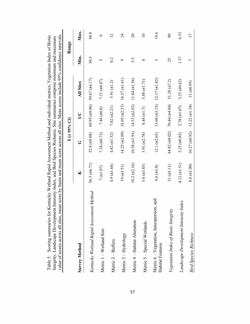
57
Tab
le 5
.
Sco
rin
g s
um
mar
ies
for
Ken
tuck
y W
etla
nd R
apid
Ass
essm
ent
Met
hod a
nd i
ndiv
idu
al m
etri
cs,
Veg
etat
ion
In
dex
of
Bio
tic
Inte
gri
ty, L
and
scap
e D
evel
opm
ent
Inte
nsi
ty I
ndex
, an
d B
ird S
pec
ies
Ric
hnes
s. S
ite
sum
mar
ies
com
pri
se m
inim
um
an
d m
axim
um
val
ue
of
score
s ac
ross
all
sit
es, m
ean s
core
by b
asin
and m
ean s
core
acr
oss
all
sit
es.
Mea
n s
core
s in
clu
de
95%
co
nfi
den
ce i
nte
rval
s.
Ra
ng
e
Ma
x.
88
.8
9
12
24
20
10
19
.6
80
6.3
3
17
Min
.
30
.5
5
0.2
9
5.5
0
3
25
1.3
7
7
x̄ (
± 9
5%
CI)
All
Sit
es
59
.67 (
±6.1
7)
7.3
1 (
±0
.47
)
5.9
1 (
±1
.2)
16
.57 (
±1.6
1)
11
.84 (
±1.5
6)
5.8
8 (
±1
.71
)
12
.17 (
±1.8
2)
51
.28 (
±7.2
)
3.2
5 (
±0
.62
)
11
(±
0.9
5)
UC
69
.95 (
±9.8
6)
7.4
4 (
±0
.8)
7.8
2 (
±2
.21
)
18
.05 (
±2.3
7)
14
.53 (
±2.8
3)
8.4
4 (
±1
.7)
13
.68 (
±3.1
5)
70
.44 (
±4.0
4)
2.7
8 (
±1
.07
)
13
.22 (
±1.3
4)
G
52
.8 (
±9
.08
)
7.3
4 (
±0
.73
)
4.8
2 (
±1
.52
)
14
.25 (
±2.0
9)
10
.38 (
±1.9
1)
3.9
1 (
±2
.78
)
12
.1 (
±2
.65
)
44
.82 (
±8.0
2)
3.2
5 (
±0
.85
)
10
.27 (
±0.9
2)
K
56
.3 (
±6
.71
)
7 (
±1
.07
)
4.9
(±
1.6
8)
19
(±
3.5
1)
10
.2 (
±2
.16
)
5.6
(±
3.8
5)
9.6
(±
3.8
)
31
(±
5.1
1)
4.1
2 (
±1
.51
)
8.6
(±
1.0
0)
Su
rvey
Met
hod
Ken
tuck
y W
etla
nd
Ra
pid
Ass
essm
ent
Met
hod
Met
ric
1 –
Wet
lan
d S
ize
Met
ric
2 –
Buff
ers
Met
ric
3 –
Hy
dro
log
y
Met
ric
4 –
Hab
itat
Alt
erat
ion
Met
ric
5 –
Spec
ial
Wet
lan
ds
Met
ric
6 –
Veg
etat
ion
, In
ters
per
sion,
and
Hab
itat
Fea
ture
s
Veg
etati
on
In
dex
of
Bio
tic
Inte
gri
ty
La
nd
sca
pe
Dev
elo
pm
ent
Inte
nsi
ty I
ndex
Bir
d S
pec
ies
Ric
hnes
s

58
Table 6. All plant species recorded at sampling sites including scientific name, common name,
family, wetland classification, and coefficient of conservatism (CofC). CofC values are ranked
from least conservative (0) to most conservative (10) (Shea et al. 2010). Invasive species (*)
are not ranked.
Scientific Name Common Name Family Wet Class CofC
Acer negundo Boxelder Maple Aceraceae Fac 1
Acer rubrum Red Maple Aceraceae Fac 3
Acer saccharinum Silver Maple Aceraceae FacW 2
Aesculus flava Yellow Sweet Buckeye Hippocastanaceae FacU 6
Aesculas glabra Ohio Buckeye Hippocastanaceae FacU 3
Agrimonia parviflora Many-flowered Agrimony Rosaceae FacW 4
Alisma subcordatum Common Water-plantain Alismataceae Obl 3
Alliaria petiolate Garlic Mustard Brassicaceae FacU *
Allium vineale Field Garlic Liliaceae FacU *
Alnus serrulata Smooth Alder Betulaceae Obl 6
Ambrosia artemisifolia Common Ragweed Asteraceae FacU 0
Ambrosia trifida Giant Ragweed Asteraceae FacU 0
Amphicarpaea
bracteata Hog-peanut Fabaceae Fac 4
Apios americana Potato-bean Fabaceae FacW 4
Arisaema dracontium Green Dragon Araceae FacW 6
Arundinaria gigantea River Cane Poaceae FacW 5
Asclepias incarnata Swamp Milkweed Asclepidaceae Obl 5
Asimina triloba North American Papaw Annonaceae FacU 7
Asplenium platyneuron Ebony spleenwort Aspleniaceae FacU 3
Aster lanceolatus Narrow-leaved Michaelmas
Daisy Asteraceae Obl 4
Aster prenanthoides Crooked-stem Aster Asteraceae Fac 5
Athyrium filix-femina Lady-fern Dryopteridaceae Fac 7
Berberis thunbergii Japanese Barberry Berberidaceae FacU *
Betula nigra River Birch Betulaceae FacW 4
Bidens connata Beggar-ticks Asteraceae FacW 5
Bidens frondosa Beggar-ticks Asteraceae FacW 1
Bignonia capreolata Cross-vine Bignoniaceae Fac 6
Boehmeria cylindrical Bog-hemp Urticaceae FacW 5
Botrychium biternatum Sparse-lobed Grape Fern Ophioglossaceae Fac 6
Botrychium virginianum Rattlesnake Fern Ophioglossaceae FacU 6
Calystegia sepium Hedge Bindweed Convolvulaceae Fac 1
Campsis radicans Trumpet Creeper Bignoniaceae Fac 1
Carex blanda Woodland Sedge Cyperaceae Fac 2
Carex conjuncta Soft Fox Sedge Cyperaceae FacW 5
Carex crinita var.
crinita Fringed Sedge Cyperaceae Obl 6

59
Table 6. Continued.
Scientific Name Common Name Family Wet Class CofC
Carex crus-corvi Raven's-foot Sedge Cyperaceae Obl 5
Carex davisii Davis' Sedge Cyperaceae Fac 5
Carex festucacea Fescue Sedge Cyperaceae Fac 7
Carex debilis var. debilis White-edged Sedge Cyperaceae Fac 7
Carex frankii Frank's Sedge Cyperaceae Obl 3
Carex gigantea Large Sedge Cyperaceae Obl 7
Carex gracillima Graceful Sedge Cyperaceae FacU 6
Carex granularis Meadow Sedge Cyperaceae FacW 5
Carex grayi Gray's Sedge Cyperaceae FacW 6
Carex grisea Narrow-leaved Sedge Cyperaceae Upl 4
Carex hirtifolia Hairy-leaved Sedge Cyperaceae Upl 7
Carex hyalinolepis Shoreline Sedge Cyperaceae Upl 5
Carex intumescens Bladder Sedge Cyperaceae FacW 6
Carex louisianica Louisiana's Sedge Cyperaceae Obl 7
Carex lupulina Hop Sedge Cyperaceae Obl 6
Carex muskingumensis Muskingum Sedge Cyperaceae Obl 8
Carex radiata Star Sedge Cyperaceae Upl 6
Carex rosea Stellate Sedge Cyperaceae Upl 5
Carex sparganoides Bur-reed Sedge Cyperaceae FacU 5
Carex squarrosa Squarrose Sedge Cyperaceae FacW 5
Carex stipata Awl-fruited Sedge Cyperaceae Obl 5
Carex swanii Swan's Sedge Cyperaceae FacU 5
Carex tribuloides Blunt Broom Sedge Cyperaceae FacW 3
Carex typhina Cattail Sedge Cyperaceae FacW 7
Carex vulpinoidea Fox Sedge Cyperaceae Obl 3
Carpinus caroliniana American Hornbeam Betulaceae Upl 6
Carya carolinae-septentrionalis Carolina Shagbark-
hickory Juglandaceae Upl 7
Carya cordiformis Bitternut Juglandaceae FacU 5
Carya laciniosa Big Shellbark Juglandaceae Fac 6
Carya ovata Shagbark Hickory Juglandaceae FacU 5
Celtis laevigata Sugarberry Ulmaceae FacW 3
Celtis occidentalis Hackberry Ulmaceae FacU 3
Cephalanthus occidentalis Buttonbush Rubiaceae Obl 3
Cercis canadensis Redbud Caesalpiniaceae FacU 3
Chasmanthium latifolium River Oats Poaceae FacU 4
Cicuta maculate Spotted Cowbane Apiaceae Obl 2

60
Table 6. Continued.
Scientific Name Common Name Family Wet Class CofC
Cinna arundinacea Wood Reedgrass Poaceae FacW 5
Circaea lutetiana Enchanter's Nightshade Onagraceae FacU 4
Commelina communis Dayflower Commelinaceae Fac *
Commelina virginica Virginia Day-flower Commelinaceae FacW 4
Cornus drummondii Rough Leaved Dogwood Cornaceae Fac 4
Cornus florida Flowering Dogwood Cornaceae FacU 5
Cryptotaenia canadensis Wild Chervil Apiaceae Fac 4
Cuscuta gronovii Love-vine Cuscutaceae Upl 4
Dicanthelium acuminatum Tall Rough Panic-grass Poaceae Fac 5
Dicanthelium clandestinum Deer Tongue Poaceae Fac 3
Dioscorea oppositifolia Chinese Yam Dioscoreaceae Upl *
Dioscorea villosa Colic-root Dioscoreaceae FacU 4
Diospyros virginiana Persimmon Ebenaceae Fac 2
Duchesnea indica Indian Strawberry Rosaceae FacU *
Elaeagnus umbellata Autumn Olive Podostemaceae Upl *
Eleocharis obtusa Blunt Spikerush Cyperaceae FacW 1
Elymus hystrix Bottlebrush Poaceae Upl 5
Elymus riparius Nodding Wild Rye Poaceae FacW 5
Elymus macgregorii Early Wild Rye Poaceae Fac 6
Elymus virginicus var. varginicus Virginia Wild Rye Poaceae Upl 5
Euonymus alatus Winged Spindle-tree Celastraceae Upl *
Euonymus fortunei Winter Creeper Celastraceae Upl *
Eupatorium coelestinum Mistflower Asteraceae Fac 3
Eupatorium fistulosum Joe-pye-weed Asteraceae FacW 5
Eupatorium perfoliatum Common Thoroughwort Asteraceae FacW 3
Fagus grandifolia American Beech Fagaceae FacU 5
Fraxinus pennsylvanica Green Ash Oleaceae FacW 3
Galium aparine Cleavers Rubiaceae FacU 0
Galium tinctorium Stiff Marsh Bedstraw Rubiaceae Obl 5
Geum canadense Wild Avens Rosaceae FacU 2
Geum virginianum Rough Avens Rosaceae Fac 5
Glechoma hederacea Ground Ivy Lamiaceae FacU *
Gleditsia triacanthos Honey-locust Caesalpiniaceae Fac 1
Glyceria septentrionalis Floating Manna-grass Poaceae Obl 7
Glyceria striata Fowl Manna-grass Poaceae Obl 4
Hamamelis virginicus Witch-hazel Hamamelidaceae FacU 6
Hibiscus laevis Halberd-leaved Rose-Mallow Malvaceae Obl 4
Houstonia purpurea Large Houstonia Rubiaceae Upl 4

61
Table 6. Continued.
Scientific Name Common Name Family Wet Class CofC
Hypericum prolificum Shrubby St. John's-wort Clusiaceae FacU 4
Ilex deciduas Possum-haw Aquifoliaceae FacW 5
Ilex opaca American Holly Aquifoliaceae FacU 5
Impatiens capensis Spotted Touch-me-not Balsaminaceae FacW 2
Iris virginica var. shrevei Southern Blue Flag Iridaceae Upl 7
Juglans nigra Black Walnut Juglandaceae FacU 4
Juncus effuses Soft Rush Juncaceae Obl 4
Juncus diffusissimus Diffuse Rush Juncaceae FacW 4
Juncus tenuis Slender Rush Juncaceae Fac 0
Juniperus virginiana Eastern Red Cedar Cupressaceae FacU 1
Leersia lenticularis Catchfly-grass Poaceae Obl 8
Leersia oryzoides Rice Cutgrass Poaceae Obl 3
Leersia virginica Cutgrass Poaceae FacW 2
Ligustrum sinense Japanese Privet Oleaceae Upl *
Lindera benzoin Spicebush Lauraceae FacW 5
Liquidambar styraciflua Sweetgum Hamamelidaceae Fac 3
Liriodendron tulipifera Tulip-poplar Magnoliaceae FacU 2
Lobelia cardinalis Cardinal-flower Campanulaceae FacW 5
Lonicera japonica Japanese Honeysuckle Caprifoliaceae Fac *
Lonicera maackii Shrub Honeysuckle Caprifoliaceae Upl *
Lonicera morrowii Shrub Honeysuckle Caprifoliaceae FacU *
Ludwigia palustris Marsh Purslane Onagraceae Obl 5
Luzula acuminate Hairy Woodrush Juncaceae Fac 5
Lycopus americanus Cut-leaved Water Hoarhound Lamiaceae Obl 4
Lycopus virginicus Spring Scorpion-grass Lamiaceae Obl 4
Lysimachia ciliate Fringed Loosestrife Primulaceae FacW 5
Lysimachia nummularia Moneywort Primulaceae FacW *
Magnolia acuminata Cucumber-tree Magnoliaceae Upl 7
Magnolia macrophyla Big-leaved Magnolia Magnoliaceae Upl 8
Magnolia tripetala Umbrella Magnolia Magnoliaceae FacU 7
Microstegium vimineum Japanese Stilt Grass Poaceae Fac *
Mimulus alatus Sharp-winged Monkey-flower Scrophulariaceae Obl 4
Morus rubra Red Mulberry Moraceae FacU 2
Nyssa sylvatica Black Tupelo Nyssaceae Fac 4
Onoclea sensibilis Sensitive Fern Dryopteridaceae FacW 4
Ostrya virginiana American Hop-hornbeam Betulaceae FacU 6
Oxalis grandis Great Yellow Wood-sorrel Oxalidaceae Upl 6
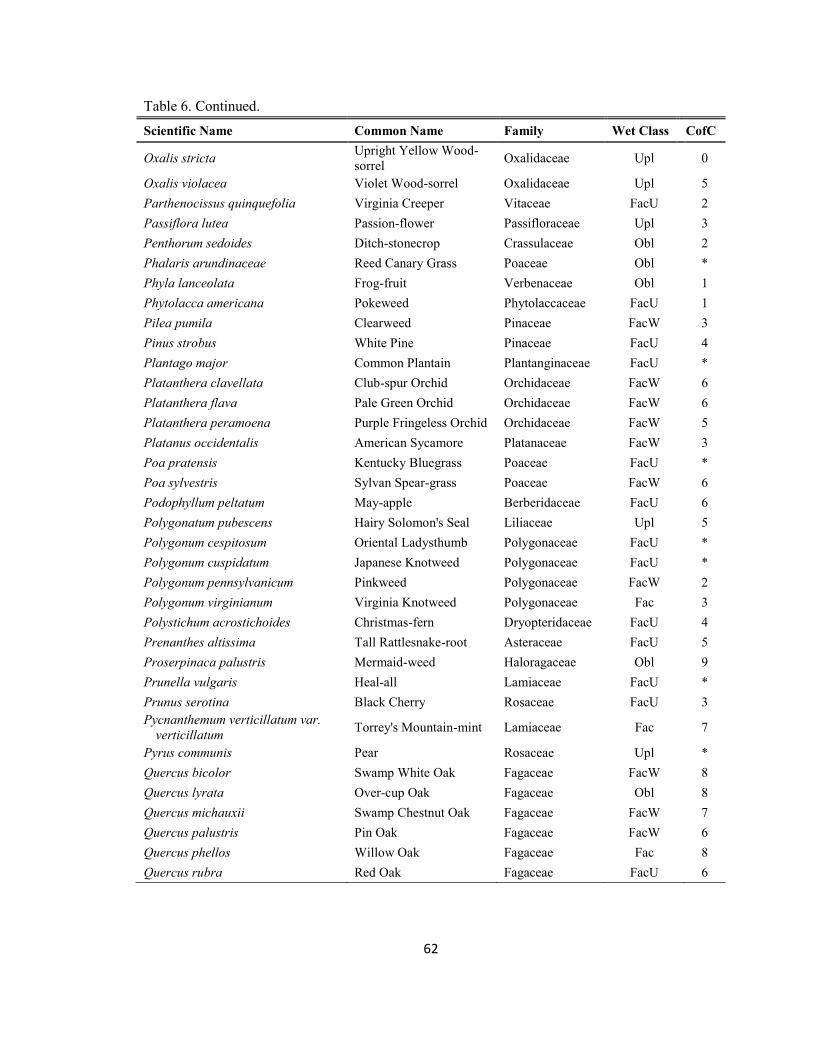
62
Table 6. Continued.
Scientific Name Common Name Family Wet Class CofC
Oxalis stricta Upright Yellow Wood-
sorrel Oxalidaceae Upl 0
Oxalis violacea Violet Wood-sorrel Oxalidaceae Upl 5
Parthenocissus quinquefolia Virginia Creeper Vitaceae FacU 2
Passiflora lutea Passion-flower Passifloraceae Upl 3
Penthorum sedoides Ditch-stonecrop Crassulaceae Obl 2
Phalaris arundinaceae Reed Canary Grass Poaceae Obl *
Phyla lanceolata Frog-fruit Verbenaceae Obl 1
Phytolacca americana Pokeweed Phytolaccaceae FacU 1
Pilea pumila Clearweed Pinaceae FacW 3
Pinus strobus White Pine Pinaceae FacU 4
Plantago major Common Plantain Plantanginaceae FacU *
Platanthera clavellata Club-spur Orchid Orchidaceae FacW 6
Platanthera flava Pale Green Orchid Orchidaceae FacW 6
Platanthera peramoena Purple Fringeless Orchid Orchidaceae FacW 5
Platanus occidentalis American Sycamore Platanaceae FacW 3
Poa pratensis Kentucky Bluegrass Poaceae FacU *
Poa sylvestris Sylvan Spear-grass Poaceae FacW 6
Podophyllum peltatum May-apple Berberidaceae FacU 6
Polygonatum pubescens Hairy Solomon's Seal Liliaceae Upl 5
Polygonum cespitosum Oriental Ladysthumb Polygonaceae FacU *
Polygonum cuspidatum Japanese Knotweed Polygonaceae FacU *
Polygonum pennsylvanicum Pinkweed Polygonaceae FacW 2
Polygonum virginianum Virginia Knotweed Polygonaceae Fac 3
Polystichum acrostichoides Christmas-fern Dryopteridaceae FacU 4
Prenanthes altissima Tall Rattlesnake-root Asteraceae FacU 5
Proserpinaca palustris Mermaid-weed Haloragaceae Obl 9
Prunella vulgaris Heal-all Lamiaceae FacU *
Prunus serotina Black Cherry Rosaceae FacU 3
Pycnanthemum verticillatum var.
verticillatum Torrey's Mountain-mint Lamiaceae Fac 7
Pyrus communis Pear Rosaceae Upl *
Quercus bicolor Swamp White Oak Fagaceae FacW 8
Quercus lyrata Over-cup Oak Fagaceae Obl 8
Quercus michauxii Swamp Chestnut Oak Fagaceae FacW 7
Quercus palustris Pin Oak Fagaceae FacW 6
Quercus phellos Willow Oak Fagaceae Fac 8
Quercus rubra Red Oak Fagaceae FacU 6

63
Table 6. Continued.
Scientific Name Common Name Family Wet Class CofC
Quercus velutina Black Oak Fagaceae Upl 5
Ranunculus hispidus Hispid Buttercup Ranunculaceae Fac 4
Rhododendron arborescens Smooth Azalea Ericaceae Fac 8
Rosa multiflora Multiflora Rose Rosaceae FacU *
Rosa palustris Swamp-rose Rosaceae Obl 6
Rubus allegheniensis Mountain Blackberry Rosaceae FacU 2
Rudbekia laciniata Green-headed
Coneflower Asteraceae FacW 5
Rumex crispus Yellow Dock Polygonaceae FacU *
Rumex obtusifolius Bitter Dock Polygonaceae FacU *
Rumex verticillatus Swamp Dock Polygonaceae Obl 5
Sagittaria latifolia Duck-potato Alismataceae Obl 4
Salix nigra Black Willow Salicaceae FacW 3
Sambucus canadensis Common Elderberry Caprifoliaceae FacW 2
Sanicula trifoliata Large-fruited Snakeroot Apiaceae Upl 4
Saururus cernuus Swamp-lily Saururaceae Obl 6
Schoenoplectus tabernaemontani Soft-stemmed Bulrush Cyperaceae Obl 3
Scirpus atrovirens Dark-green Bulrush Cyperaceae Obl 3
Scirpus georgianus Dark-green Bulrush Cyperaceae Obl 3
Scirpus polyphyllus Leafy Bulrush Cyperaceae Obl 3
Scutellaria lateriflora Mad-dog Skullcap Lamiaceae FacW 5
Sedum ternatum Wild Stonecrop Crassulaceae Upl 5
Senico aureus Golden Ragwort Asteraceae FacW 5
Senico glabellus Butterweed Asteraceae Obl 2
Silphium perfoliatum Cup-plant Asteraceae FacU 6
Sium suave Hemlock Apiaceae Obl 6
Smilax glauca Sawbrier Smilacaceae FacU 3
Smilax hispida Hispid Greenbrier Smilacaceae Fac 3
Smilax rotundifolia Common Greenbrier Smilacaceae Fac 4
Solanum carolinense Horse-nettle Solanaceae Upl *
Solidago canadensis Canada Goldenrod Asteraceae Upl 4
Sorghum halepense Johnson-grass Poaceae FacU *
Stachys tenuifolia Hedge Nettle Lamiaceae Obl 4
Symphiocarpus orbiculatus Coralberry Caprifoliaceae Upl 2
Thalictrum pubescens Tall Meadow-rue Ranunculaceae FacW 4
Thalictrum thalictroides Rue-anemone Ranunculaceae FacU 5
Thelypteris noveboracensis New York Fern Thelypteridaceae Fac 5
Toxicodendron radicans Poison Ivy Anacardiaceae Fac 2

64
Table 6. Continued.
Scientific Name Common Name Family Wet Class CofC
Tradescantia subaspera var. montana Zigzag Spiderwort Commelinaceae Upl 7
Trillium erectum Purple Trillium Liliaceae FacU 6
Tsuga canadensis Eastern Hemlock Pinaceae FacU 6
Typha latifolia Common Cat-tail Typhaceae Obl 1
Ulmus americana American Elm Ulmaceae FacW 5
Ulmus rubra Slippery Elm Ulmaceae Fac 4
Urtica dioica Stinging Nettle Urticaceae FacU 4
Verbesina alternifolia Wingstem Asteraceae Fac 2
Vernonia gigantea Tall Ironweed Asteraceae Fac 2
Viburnum dentatum Southern Arrow-wood Caprifoliaceae Fac 7
Viburnum rufidulum Southern Black-haw Caprifoliaceae Upl 4
Viola canadensis Canada Violet Violaceae Upl 6
Viola cucullata Marsh Blue Violet Violaceae FacW 4
Vitis aestivalis Summer Grape Vitaceae FacU 3
Vitis cinerea Graybark Grape Vitaceae FacW 3
Vitis riparia Frost Grape Vitaceae FacW 4
Xanthium strumarium Common Cocklebur Asteraceae Fac *
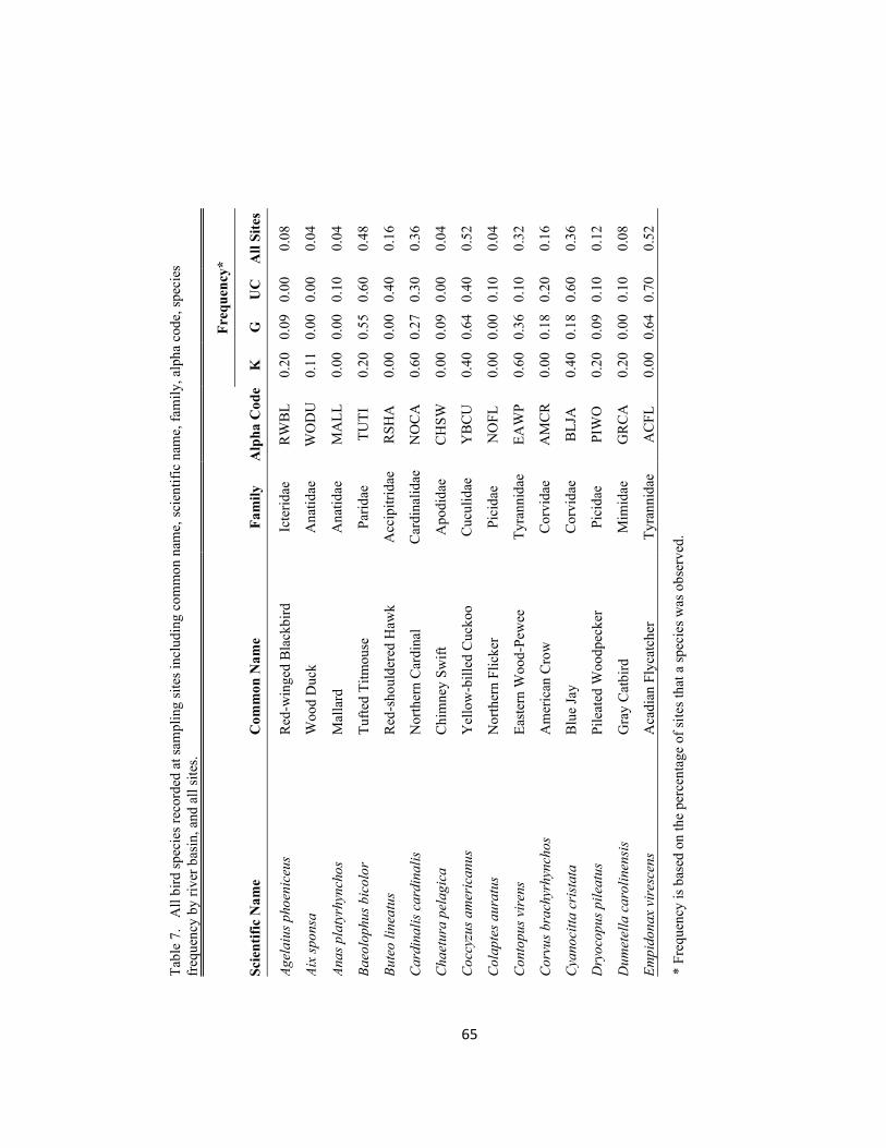
65
Tab
le 7
.
All
bir
d s
pec
ies
reco
rded
at
sam
pli
ng
sit
es i
ncl
ud
ing
co
mm
on
nam
e, s
cien
tifi
c n
ame,
fam
ily
, al
ph
a co
de,
sp
ecie
s
freq
uen
cy b
y r
iver
bas
in,
and
all
sit
es.
Fre
qu
ency
* A
ll S
ites
0.0
8
0.0
4
0.0
4
0.4
8
0.1
6
0.3
6
0.0
4
0.5
2
0.0
4
0.3
2
0.1
6
0.3
6
0.1
2
0.0
8
0.5
2
UC
0.0
0
0.0
0
0.1
0
0.6
0
0.4
0
0.3
0
0.0
0
0.4
0
0.1
0
0.1
0
0.2
0
0.6
0
0.1
0
0.1
0
0.7
0
G
0.0
9
0.0
0
0.0
0
0.5
5
0.0
0
0.2
7
0.0
9
0.6
4
0.0
0
0.3
6
0.1
8
0.1
8
0.0
9
0.0
0
0.6
4
K
0.2
0
0.1
1
0.0
0
0.2
0
0.0
0
0.6
0
0.0
0
0.4
0
0.0
0
0.6
0
0.0
0
0.4
0
0.2
0
0.2
0
0.0
0
Alp
ha
Co
de
RW
BL
WO
DU
MA
LL
TU
TI
RS
HA
NO
CA
CH
SW
YB
CU
NO
FL
EA
WP
AM
CR
BL
JA
PIW
O
GR
CA
AC
FL
Fa
mil
y
Icte
rid
ae
An
atid
ae
An
atid
ae
Par
idae
Acc
ipit
rid
ae
Car
din
alid
ae
Ap
od
idae
Cu
culi
dae
Pic
idae
Ty
ran
nid
ae
Co
rvid
ae
Co
rvid
ae
Pic
idae
Mim
idae
Ty
ran
nid
ae
* F
req
uen
cy i
s b
ased
on
th
e per
cen
tag
e of
site
s th
at a
sp
ecie
s w
as o
bse
rved
.
Co
mm
on
Na
me
Red
-win
ged
Bla
ckb
ird
Wo
od
Du
ck
Mal
lard
Tu
fted
Tit
mou
se
Red
-sh
ou
lder
ed H
awk
No
rth
ern
Car
din
al
Ch
imn
ey S
wif
t
Yel
low
-bil
led
Cu
cko
o
No
rth
ern
Fli
cker
Eas
tern
Wo
od
-Pew
ee
Am
eric
an C
row
Blu
e Ja
y
Pil
eate
d W
oo
dp
eck
er
Gra
y C
atb
ird
Aca
dia
n F
lyca
tch
er
Sci
enti
fic
Na
me
Ag
ela
ius
pho
enic
eus
Aix
sp
on
sa
An
as
pla
tyrh
ynch
os
Ba
eolo
ph
us
bic
olo
r
Bu
teo
lin
eatu
s
Ca
rdin
ali
s ca
rdin
ali
s
Ch
aet
ura
pel
ag
ica
Co
ccyz
us
am
eric
an
us
Co
lap
tes
au
ratu
s
Co
nto
pu
s vi
ren
s
Co
rvu
s b
rach
yrh
ynch
os
Cya
no
citt
a c
rist
ata
Dry
oco
pu
s p
ilea
tus
Du
met
ella
ca
roli
nen
sis
Em
pid
on
ax
vire
scen
s

66
Tab
le 7
.
Con
tin
ued
.
Fre
qu
ency
* A
ll S
ites
0.0
4
0.0
4
0.2
8
0.0
4
0.0
4
0.0
4
0.2
0
0.0
8
0.1
6
0.3
6
0.2
0
0.4
8
0.4
4
0.1
2
0.2
4
UC
0.0
0
0.1
0
0.7
0
0.0
0
0.1
0
0.1
0
0.3
0
0.1
0
0.4
0
0.9
0
0.2
0
0.3
0
0.2
0
0.1
0
0.4
0
G
0.0
9
0.0
0
0.0
0
0.0
0
0.0
0
0.0
0
0.1
8
0.0
9
0.0
0
0.0
9
0.1
8
0.7
3
0.6
4
0.1
8
0.1
8
K
0.0
0
0.0
0
0.2
0
0.2
0
0.0
0
0.0
0
0.0
0
0.0
0
0.0
0
0.0
0
0.2
0
0.2
0
0.4
0
0.0
0
0.0
0
Alp
ha
Co
de
CO
YE
WE
WA
WO
TH
YB
CH
BA
OR
SW
WA
RB
WO
SO
SP
GC
FL
KE
WA
LO
WA
NO
PA
INB
U
DO
WO
EA
TO
Fa
mil
y
Par
uli
dae
Par
uli
dae
Tu
rdid
ae
Par
uli
dae
Icte
rid
ae
Par
uli
dae
Pic
idae
Em
ber
izid
ae
Ty
ran
nid
ae
Par
uli
dae
Par
uli
dae
Par
uli
dae
Car
din
alid
ae
Pic
idae
Em
ber
izid
ae
* F
req
uen
cy i
s b
ased
on
th
e per
cen
tag
e of
site
s th
at a
sp
ecie
s w
as o
bse
rved
Co
mm
on
Na
me
Co
mm
on
Yel
low
thro
at
Wo
rm-e
atin
g W
arb
ler
Wo
od
Th
rush
Yel
low
-bre
aste
d C
hat
Bal
tim
ore
Ori
ole
Sw
ain
son
's W
arb
ler
Red
-bel
lied
Wo
od
pec
ker
So
ng
Sp
arro
w
Gre
at C
rest
ed F
lyca
tch
er
Ken
tuck
y W
arb
ler
Lo
uis
ian
a W
ater
thru
sh
No
rth
ern
Par
ula
Ind
igo B
un
tin
g
Do
wn
y W
oo
dp
eck
er
Eas
tern
To
wh
ee
Sci
enti
fic
Na
me
Geo
thly
pis
tri
cha
s
Hel
mit
her
os
verm
ivo
rus
Hyl
oci
chla
mu
stel
ina
Icte
ria
vir
ens
Icte
rus
gla
bu
la
Lim
no
thly
pis
sw
ain
son
ii
Mel
an
erp
es c
aro
lin
us
Mel
osp
iza
mel
od
ia
Myi
arc
hu
s cr
init
us
Op
oro
nis
fo
rmo
sus
Pa
rkes
ia m
ota
cill
a
Pa
rula
am
eric
an
a
Pa
sser
ina
cya
nea
Pic
oid
es p
ub
esce
ns
Pip
ilo
ert
hro
ph
tha
lmu
s

67
Tab
le 7
.
Con
tin
ued
.
Fre
qu
ency
* A
ll S
ites
0.0
8
0.1
6
0.6
0
0.5
2
0.2
8
0.0
4
0.5
2
0.2
4
0.0
4
0.0
4
0.2
0
0.2
4
0.0
4
0.6
0
0.0
8
UC
0.2
0
0.1
0
0.4
0
0.7
0
0.0
0
0.1
0
0.9
0
0.1
0
0.1
0
0.0
0
0.2
0
0.1
0
0.0
0
0.3
0
0.0
0
G
0.0
0
0.2
7
0.6
4
0.5
5
0.6
4
0.0
0
0.3
6
0.2
7
0.0
0
0.0
9
0.0
9
0.4
5
0.0
9
0.7
3
0.0
0
K
0.0
0
0.0
0
0.8
0
0.2
0
0.0
0
0.0
0
0.2
0
0.4
0
0.0
0
0.0
0
0.4
0
0.0
0
0.0
0
0.8
0
0.4
0
Alp
ha
Co
de
SC
TA
SU
TA
CA
CH
BG
GN
PR
OW
EA
PH
OV
EN
YT
WA
BT
NW
EA
BL
WB
NU
AM
GO
FIS
P
CA
RW
HO
WR
Fa
mil
y
Th
rau
pid
ae
Th
rau
pid
ae
Par
idae
Po
lio
pti
lid
ae
Par
uli
dae
Ty
ran
nid
ae
Par
uli
dae
Par
uli
dae
Par
uli
dae
Tu
rdid
ae
Sit
tid
ae
Fri
ng
illi
dae
Em
ber
izid
ae
Tro
glo
dy
tid
ae
Tro
glo
dy
tid
ae
* F
req
uen
cy i
s b
ased
on
th
e per
cen
tag
e of
site
s th
at a
sp
ecie
s w
as o
bse
rved
Co
mm
on
Na
me
Sca
rlet
Tan
ager
Su
mm
er T
anag
er
Car
oli
na
Ch
ick
adee
Blu
e-g
ray
Gn
atca
tch
er
Pro
tho
no
tary
War
ble
r
Eas
tern
Ph
oeb
e
Ov
enb
ird
Yel
low
-th
roat
ed W
arb
ler
Bla
ck-t
hro
ated
Gre
en W
arb
ler
Eas
tern
Blu
ebir
d
Wh
ite-
bre
aste
d N
uth
atch
Am
eric
an G
old
fin
ch
Fie
ld S
par
row
Car
oli
na
Wre
n
Ho
use
Wre
n
Sci
enti
fic
Na
me
Pir
an
ga
oli
vace
a
Pir
an
ga
ru
bra
Po
ecil
e ca
roli
nen
sis
Po
lio
pti
la c
aer
ule
a
Pro
ton
ota
ria
cit
rea
Sa
yorn
is p
ho
ebe
Sei
uru
s a
uro
cap
illa
Set
op
ha
ga
do
min
ica
Set
op
ha
ga
vir
ens
Sia
lia
sia
lis
Sit
ta c
aro
lin
ensi
s
Sp
inu
s tr
isti
s
Sp
izel
la p
usi
lla
Th
ryo
tho
rus
lud
ovi
cia
nu
s
Tro
glo
dyt
es a
edo
n

68
Tab
le 7
.
Con
tin
ued
.
Fre
qu
ency
* A
ll S
ites
0.1
6
0.0
4
0.1
6
0.4
8
0.2
0
0.0
8
UC
0.1
0
0.1
0
0.3
0
0.6
0
0.6
0
0.1
0
G
0.0
0
0.0
0
0.0
9
0.4
5
0.0
0
0.0
9
K
0.6
0
0.0
0
0.0
0
0.4
0
0.0
0
0.0
0
Alp
ha
Co
de
AM
RO
BW
WA
WE
VI
RE
VI
HO
WA
MO
DO
* F
req
uen
cy i
s b
ased
on
th
e per
cen
tag
e of
site
s th
at a
sp
ecie
s w
as o
bse
rved
Fa
mil
y
Tu
rdid
ae
Par
uli
dae
Vir
eon
idae
Vir
eon
idae
Par
uli
dae
Co
lum
bid
ae
Co
mm
on
Na
me
Am
eric
an R
ob
in
Blu
e-w
ing
ed W
arb
ler
Wh
ite-
eyed
Vir
eo
Red
-ey
ed V
ireo
Ho
od
ed W
arb
ler
Mo
urn
ing
Do
ve
Sci
enti
fic
Na
me
Tu
rdu
s m
igra
tori
us
Ver
miv
ora
pin
us
Vir
eo g
rise
us
Vir
eo o
liva
ceu
s
Wil
son
ia c
itri
na
Zen
aid
a m
aa
crou
ra

69
APPENDIX B
Regressions Figures

70
Figure 6a. Linear regression between the KY-WRAM score and LDI score.
Different symbols represent river basin for each site.

71
Figure 6b. Linear regression between the KY-WRAM score and VIBI score.
Different symbols represent river basin for each site.

72
Figure 6c. Linear regression between KY-WRAM score and bird species
richness. Different symbols represent river basin for each site.

73
APPENDIX C
AIC Models and Parameter Estimates

74
Table 8a. Model selection for the effects of vegetation and land use variables on wetland size and
distribution (Metric 1).
Model K AICc ∆AICc ω LL
fqai 3 84.69 0.00 0.14 -38.77
ldi 3 85.41 0.73 0.10 -39.14
%cultivated 3 85.59 0.90 0.09 -39.22
%forested 3 85.64 0.95 0.09 -39.25
%adventive 3 85.65 0.96 0.09 -39.25
stems 3 85.65 0.96 0.09 -39.25
fqai + ldi 4 86.90 2.21 0.05 -38.45
fqai + %cultivated 4 87.15 2.46 0.04 -38.57
fqai + %forested 4 87.22 2.54 0.04 -38.61
fqai + stems 4 87.52 2.84 0.03 -38.76
fqai + %adventive 4 87.54 2.85 0.03 -38.77
ldi + stems 4 88.25 3.56 0.02 -39.12
%adventive + ldi 4 88.26 3.57 0.02 -39.13
%cultivated + ldi 4 88.27 3.58 0.02 -39.13
%cultivated + stems 4 88.42 3.73 0.02 -39.21
%cultivated + %adventive 4 88.43 3.75 0.02 -39.22
%adventive + %forested 4 88.47 3.79 0.02 -39.24
fqai + %cultivated + ldi 5 89.96 5.28 0.01 -38.40
fqai + ldi + %forested 5 90.02 5.33 0.01 -38.43
fqai + %cultivated + stems 5 90.26 5.57 0.01 -38.55
fqai + %cultivated + %adventive 5 90.31 5.62 0.01 -38.57
fqai + %forested + stems 5 90.34 5.65 0.01 -38.59
%cultivated + ldi + %forested 5 91.02 6.33 0.01 -38.93
ldi + %forested + stems 5 91.15 6.47 0.01 -39.00
%cultivated + ldi + stems 5 91.40 6.71 0.00 -39.12
%cultivated + %adventive + ldi 5 91.42 6.73 0.00 -39.12
%cultivated + %forested + stems 5 91.58 6.89 0.00 -39.21
fqai + %cultivated + %forested + %adventive + ldi + stems 8 101.51 16.82 0.00 -38.25
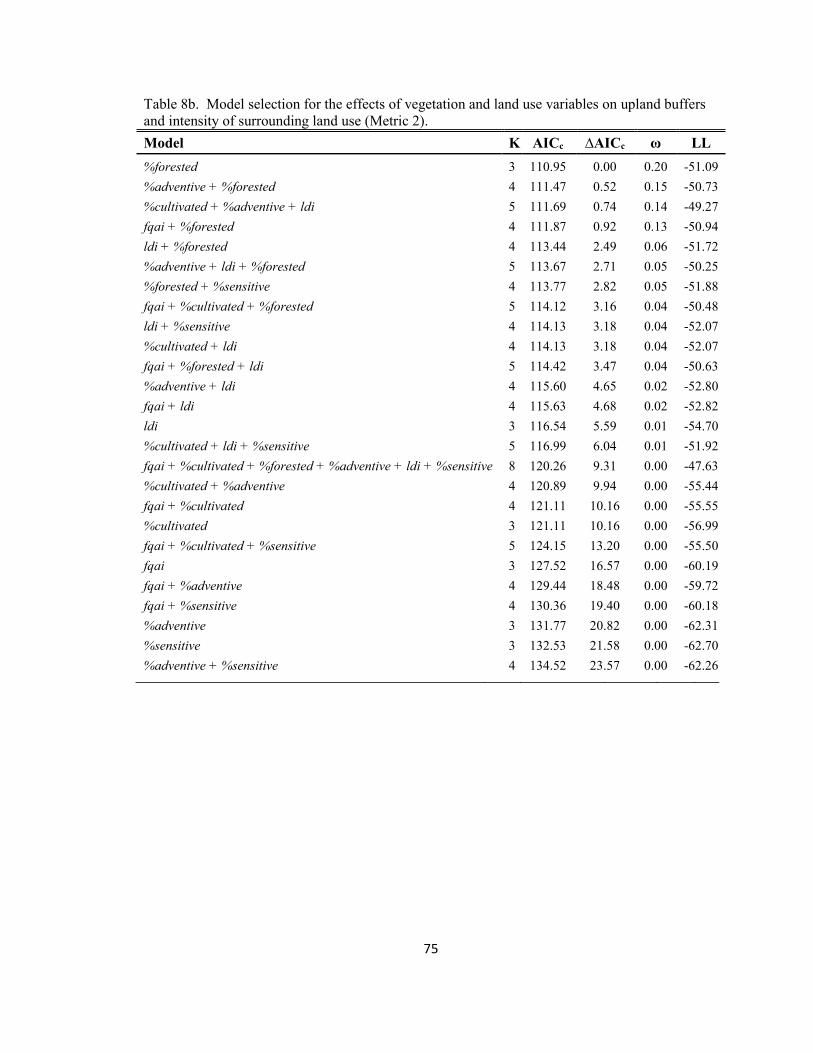
75
Table 8b. Model selection for the effects of vegetation and land use variables on upland buffers
and intensity of surrounding land use (Metric 2).
Model K AICc ∆AICc ω LL
%forested 3 110.95 0.00 0.20 -51.09
%adventive + %forested 4 111.47 0.52 0.15 -50.73
%cultivated + %adventive + ldi 5 111.69 0.74 0.14 -49.27
fqai + %forested 4 111.87 0.92 0.13 -50.94
ldi + %forested 4 113.44 2.49 0.06 -51.72
%adventive + ldi + %forested 5 113.67 2.71 0.05 -50.25
%forested + %sensitive 4 113.77 2.82 0.05 -51.88
fqai + %cultivated + %forested 5 114.12 3.16 0.04 -50.48
ldi + %sensitive 4 114.13 3.18 0.04 -52.07
%cultivated + ldi 4 114.13 3.18 0.04 -52.07
fqai + %forested + ldi 5 114.42 3.47 0.04 -50.63
%adventive + ldi 4 115.60 4.65 0.02 -52.80
fqai + ldi 4 115.63 4.68 0.02 -52.82
ldi 3 116.54 5.59 0.01 -54.70
%cultivated + ldi + %sensitive 5 116.99 6.04 0.01 -51.92
fqai + %cultivated + %forested + %adventive + ldi + %sensitive 8 120.26 9.31 0.00 -47.63
%cultivated + %adventive 4 120.89 9.94 0.00 -55.44
fqai + %cultivated 4 121.11 10.16 0.00 -55.55
%cultivated 3 121.11 10.16 0.00 -56.99
fqai + %cultivated + %sensitive 5 124.15 13.20 0.00 -55.50
fqai 3 127.52 16.57 0.00 -60.19
fqai + %adventive 4 129.44 18.48 0.00 -59.72
fqai + %sensitive 4 130.36 19.40 0.00 -60.18
%adventive 3 131.77 20.82 0.00 -62.31
%sensitive 3 132.53 21.58 0.00 -62.70
%adventive + %sensitive 4 134.52 23.57 0.00 -62.26

76
Table 8c. Model selection for the effects of vegetation and land use variables on wetland
hydrology (Metric 3).
Model K AICc ∆AICc ω LL
ldi 3 145.03 0.00 0.19 -68.94
%hydrophyte 3 146.87 1.84 0.08 -69.86
fqai 3 146.98 1.95 0.07 -69.92
stems 3 147.26 2.23 0.06 -70.06
%hydrophyte + ldi 4 147.27 2.24 0.06 -68.64
hydro sr 3 147.47 2.44 0.06 -70.16
carex sr 3 147.53 2.50 0.05 -70.19
ldi + stems 4 147.63 2.60 0.05 -68.82
ldi + hydro sr 4 147.71 2.68 0.05 -68.85
fqai + ldi 4 147.73 2.70 0.05 -68.87
ldi + carex sr 4 147.89 2.86 0.05 -68.94
fqai + hydro sr 4 149.36 4.33 0.02 -69.68
fqai + carex sr 4 149.50 4.47 0.02 -69.75
stems + %hydrophyte 4 149.50 4.47 0.02 -69.75
fqai + stems 4 149.52 4.49 0.02 -69.76
hydro sr + %hydrophyte 4 149.65 4.62 0.02 -69.82
carex sr + %hydrophyte 4 149.67 4.64 0.02 -69.84
fqai + hydro sr 4 149.81 4.78 0.02 -69.90
stems + carex sr 4 150.06 5.03 0.02 -70.03
stems + hydro sr 4 150.08 5.05 0.02 -70.04
carex sr + hydro sr 4 150.23 5.20 0.01 -70.11
ldi + hydro sr + %hydrophyte 5 150.27 5.24 0.01 -68.56
fqai + ldi + carex sr 5 150.84 5.81 0.01 -68.84
fqai + stems + carex sr 5 152.25 7.22 0.01 -69.55
fqai + hydro sr + %hydrophyte 5 152.51 7.48 0.00 -69.68
stems + hydro sr + %hydrophyte 5 152.62 7.59 0.00 -69.73
carex sr + hydro sr + %hydrophyte 5 152.68 7.65 0.00 -69.76
ldi + carex sr + hydro sr 5 152.68 7.65 0.00 -69.76
fqai + ldi + stems + carex sr + hydro sr + %hydrophyte 8 161.91 16.88 0.00 -68.46
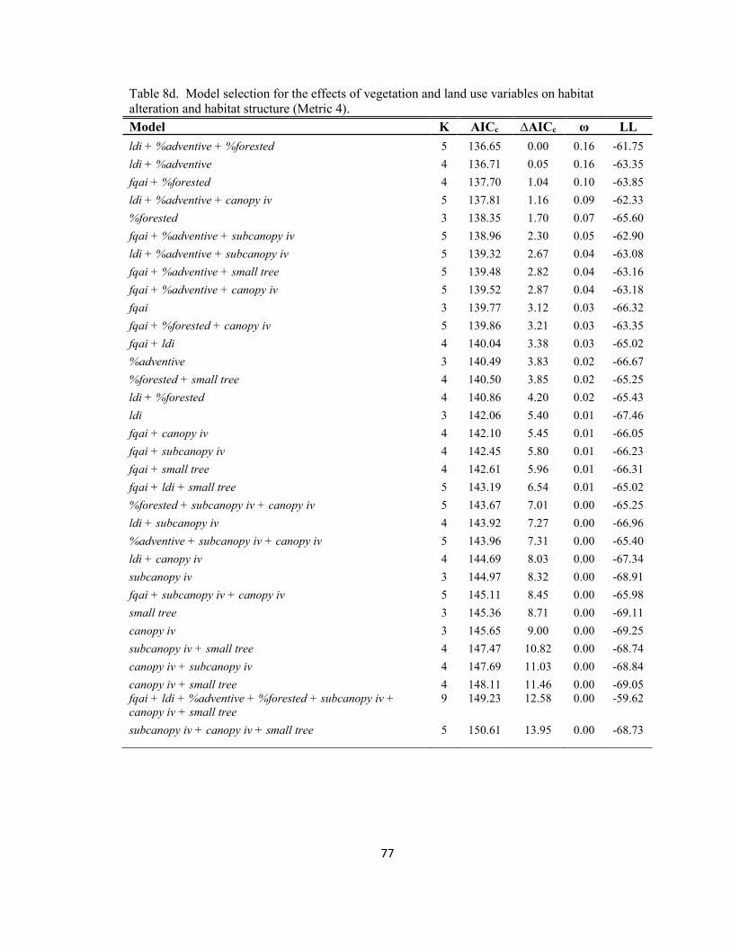
77
Table 8d. Model selection for the effects of vegetation and land use variables on habitat
alteration and habitat structure (Metric 4).
Model K AICc ∆AICc ω LL
ldi + %adventive + %forested 5 136.65 0.00 0.16 -61.75
ldi + %adventive 4 136.71 0.05 0.16 -63.35
fqai + %forested 4 137.70 1.04 0.10 -63.85
ldi + %adventive + canopy iv 5 137.81 1.16 0.09 -62.33
%forested 3 138.35 1.70 0.07 -65.60
fqai + %adventive + subcanopy iv 5 138.96 2.30 0.05 -62.90
ldi + %adventive + subcanopy iv 5 139.32 2.67 0.04 -63.08
fqai + %adventive + small tree 5 139.48 2.82 0.04 -63.16
fqai + %adventive + canopy iv 5 139.52 2.87 0.04 -63.18
fqai 3 139.77 3.12 0.03 -66.32
fqai + %forested + canopy iv 5 139.86 3.21 0.03 -63.35
fqai + ldi 4 140.04 3.38 0.03 -65.02
%adventive 3 140.49 3.83 0.02 -66.67
%forested + small tree 4 140.50 3.85 0.02 -65.25
ldi + %forested 4 140.86 4.20 0.02 -65.43
ldi 3 142.06 5.40 0.01 -67.46
fqai + canopy iv 4 142.10 5.45 0.01 -66.05
fqai + subcanopy iv 4 142.45 5.80 0.01 -66.23
fqai + small tree 4 142.61 5.96 0.01 -66.31
fqai + ldi + small tree 5 143.19 6.54 0.01 -65.02
%forested + subcanopy iv + canopy iv 5 143.67 7.01 0.00 -65.25
ldi + subcanopy iv 4 143.92 7.27 0.00 -66.96
%adventive + subcanopy iv + canopy iv 5 143.96 7.31 0.00 -65.40
ldi + canopy iv 4 144.69 8.03 0.00 -67.34
subcanopy iv 3 144.97 8.32 0.00 -68.91
fqai + subcanopy iv + canopy iv 5 145.11 8.45 0.00 -65.98
small tree 3 145.36 8.71 0.00 -69.11
canopy iv 3 145.65 9.00 0.00 -69.25
subcanopy iv + small tree 4 147.47 10.82 0.00 -68.74
canopy iv + subcanopy iv 4 147.69 11.03 0.00 -68.84
canopy iv + small tree 4 148.11 11.46 0.00 -69.05
fqai + ldi + %adventive + %forested + subcanopy iv +
canopy iv + small tree
9
149.23
12.58
0.00
-59.62
subcanopy iv + canopy iv + small tree 5 150.61 13.95 0.00 -68.73

78
Table 8e. Model selection for the effects of vegetation and land use variables on special wetlands
(Metric 5).
Model K AICc ∆AICc ω LL
%sensitive 3 148.89 0.00 0.12 -70.87
fqai 3 149.07 0.18 0.11 -70.96
%cultivated 3 149.45 0.56 0.09 -71.15
dicot sr 3 149.69 0.80 0.08 -71.28
carex sr 3 149.99 1.10 0.07 -71.42
ldi 3 150.50 1.60 0.06 -71.68
%adventive 3 150.50 1.61 0.06 -71.68
fqai + %sensitive 4 150.97 2.08 0.04 -70.49
fqai + %cultivated 4 151.37 2.48 0.04 -70.69
%sensitive + %adventive 4 151.75 2.86 0.03 -70.87
carex sr + dicot sr 4 151.79 2.90 0.03 -70.90
fqai + carex sr 4 151.85 2.96 0.03 -70.92
fqai + %adventive 4 151.87 2.98 0.03 -70.94
fqai + dicot sr 4 151.91 3.02 0.03 -70.96
fqai + ldi 4 151.93 3.03 0.03 -70.96
ldi + %cultivated 4 152.26 3.37 0.02 -71.13
ldi + dicot sr 4 152.53 3.64 0.02 -71.27
ldi + carex sr 4 152.66 3.77 0.02 -71.33
fqai + %sensitive + %cultivated 5 153.27 4.38 0.01 -70.06
ldi + %sensitive + %cultivated 5 153.34 4.45 0.01 -70.09
%sensitive + %cultivated + %adventive 5 153.54 4.65 0.01 -70.19
%sensitive + carex sr + dicot sr 5 154.00 5.11 0.01 -70.42
fqai + %sensitive + carex sr 5 154.13 5.24 0.01 -70.49
fqai + ldi + %cultivated 5 154.41 5.52 0.01 -70.63
%adventive + carex sr + dicot sr 5 154.84 5.95 0.01 -70.84
fqai + carex sr + dicot sr 5 154.87 5.98 0.01 -70.86
fqai + ldi + %adventive 5 155.03 6.14 0.01 -70.93
ldi + %cultivated + %adventive 5 155.23 6.34 0.01 -71.03
fqai + ldi + %sensitive + %cultivated + %adventive +
carex sr + dicot sr
9
169.29
20.40
0.00
-69.65

79
Table 8f. Model selection for the effects of vegetation and land use variables on vegetation,
interspersion, and habitat features (Metric 6).
Model K AICc ∆AICc ω LL
%adventive + carex sr 4 136.51 0.00 0.27 -63.25
%adventive + ldi + carex sr 5 137.04 0.53 0.21 -61.94
fqai + %adventive 4 137.62 1.12 0.16 -63.81
fqai + %adventive + carex sr 5 137.75 1.24 0.15 -62.29
%adventive 3 139.59 3.09 0.06 -66.22
fqai + %cultivated + %adventive 5 139.81 3.30 0.05 -63.32
%cultivated + %adventive 4 140.03 3.52 0.05 -65.01
%adventive + ldi 4 140.99 4.49 0.03 -65.50
%cultivated + %adventive + ldi 5 142.89 6.38 0.01 -64.86
fqai + %cultivated + %adventive + ldi + carex sr 7 143.09 6.59 0.01 -61.25
carex sr 3 145.40 8.89 0.00 -69.13
ldi + carex sr 4 147.08 10.58 0.00 -68.54
fqai + carex sr 4 147.48 10.98 0.00 -68.74
%cultivated + carex sr 4 147.60 11.10 0.00 -68.80
fqai + ldi + carex sr 5 149.94 13.43 0.00 -68.39
fqai 3 150.11 13.60 0.00 -71.48
%cultivated + ldi + carex sr 5 150.14 13.63 0.00 -68.49
fqai + %cultivated + carex sr 5 150.33 13.82 0.00 -68.58
fqai + %cultivated 4 152.89 16.39 0.00 -71.45
fqai + ldi 4 152.95 16.44 0.00 -71.47
%cultivated 3 153.07 16.56 0.00 -72.96
ldi 3 153.38 16.87 0.00 -73.28
%cultivated + ldi 4 155.87 19.36 0.00 -72.93
fqai + %cultivated + ldi 5 156.05 19.54 0.00 -71.45
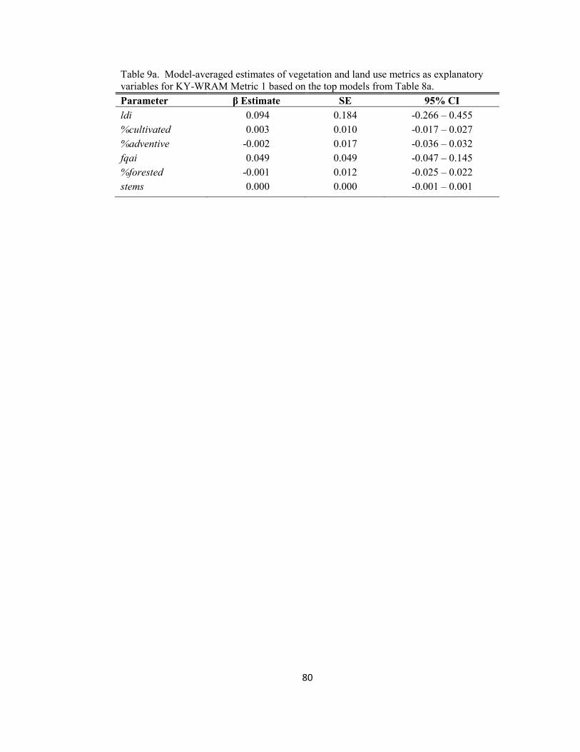
80
Table 9a. Model-averaged estimates of vegetation and land use metrics as explanatory
variables for KY-WRAM Metric 1 based on the top models from Table 8a.
Parameter β Estimate SE 95% CI
ldi 0.094 0.184 -0.266 – 0.455
%cultivated 0.003 0.010 -0.017 – 0.027
%adventive -0.002 0.017 -0.036 – 0.032
fqai 0.049 0.049 -0.047 – 0.145
%forested -0.001 0.012 -0.025 – 0.022
stems 0.000 0.000 -0.001 – 0.001

81
Table 9b. Model-averaged estimates of vegetation and land use metrics as explanatory
variables for KY-WRAM Metric 2 based on the top models from Table 8b. Metrics
labelled with a (*) were statistically significant, and confidence intervals do not overlap
zero.
Parameter β Estimate SE 95% CI
fqai 0.116 0.086 -0.053 – 0.284
ldi -0.831 0.515 -1.840 – 0.178
%cultivated -0.041 0.021 -0.081 – 0.000
%forested* 0.080 0.022 0.038 – 0.123
%sensitive 0.006 0.026 -0.046 – 0.057
%adventive -0.051 0.030 -0.109 – 0.007

82
Table 9c. Model-averaged estimates of vegetation and land use metrics as explanatory
variables for KY-WRAM Metric 3 based on the top models from Table 8c.
Parameter β Estimate SE 95% CI
ldi -0.797 0.525 -1.826 – 0.232
%hydrophyte -0.031 0.041 -0.112 – 0.050
fqai 0.109 0.176 -0.236 – 0.454
carex sr -0.065 0.305 -0.663 – 0.534
hydro sr 0.035 0.136 -0.232 – 0.301
stems 0.001 0.001 -0.002 – 0.003

83
Table 9d. Model-averaged estimates of vegetation and land use metrics as explanatory
variables for KY-WRAM Metric 4 based on the top models from Table 8d. Metrics
labelled with a (*) were statistically significant, and confidence intervals do not overlap
zero.
Parameter β Estimate SE 95% CI
subcanopy iv -0.418 12.554 -25.024 – 24.188
canopy iv -9.049 28.208 -64.337 – 46.238
fqai* 0.330 0.160 0.016 – 0.644
ldi -0.636 0.805 -2.214 – 0.925
small tree -1.009 8.990 -18.628 – 16.610
%forested -0.074 0.039 -0.004 – 0.150
%adventive* -0.129 0.048 -0.224 – -0.035

84
Table 9e. Model-averaged estimates of vegetation and land use metrics as explanatory
variables for KY-WRAM Metric 5 based on the top models from Table 8e.
Parameter β Estimate SE 95% CI
ldi -0.041 0.627 -1.271 – 1.188
%sensitive 0.064 0.056 -0.045 – 0.173
%cultivated -0.035 0.037 -0.107 – 0.037
%adventive -0.013 0.064 -0.139 – 0.113
fqai 0.181 0.191 -0.193 – 0.556
carex sr 0.193 0.331 -0.456 – 0.842
dicot sr -0.085 0.121 -0.152 – 0.322

85
Table 9f. Model-averaged estimates of vegetation and land use metrics as explanatory
variables for KY-WRAM Metric 6 based on the top models from Table 8f. Metrics
labelled with a (*) were statistically significant, and confidence intervals do not overlap
zero.
Parameter β Estimate SE 95% CI
%adventive* -0.189 0.051 -0.288 – -0.090
ldi -0.589 0.437 -1.445 – 0.267
carex sr* 0.552 0.252 0.058 – 1.047
%cultivated -0.032 0.030 -0.090 – 0.026
fqai 0.231 0.145 -0.055 – 0.517

86
APPENDIX D
PCA Eigenvalues, Variance, and Loading Values

87
Table 10a. Principal Component Analysis eigenvalues and the proportional
and cumulative variation of axes for Figure 8. Two axes explained 51.2% of
the variation present in the sampled data of KY-WRAM metrics.
PC1 PC2
Eigenvalue 2.350 1.741
Proportion Explained 0.294 0.218
Cumulative Proportion 0.294 0.512
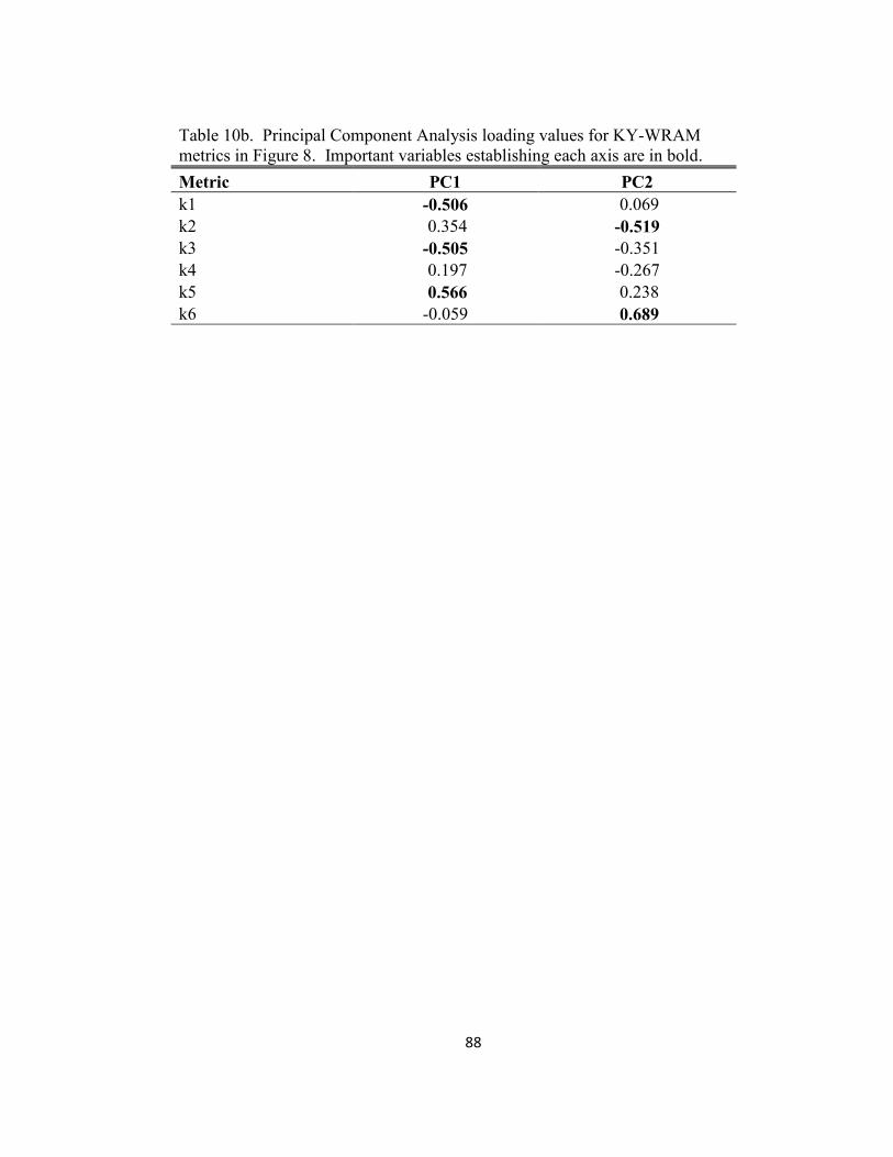
88
Table 10b. Principal Component Analysis loading values for KY-WRAM
metrics in Figure 8. Important variables establishing each axis are in bold.
Metric PC1 PC2
k1 -0.506 0.069
k2 0.354 -0.519
k3 -0.505 -0.351
k4 0.197 -0.267
k5 0.566 0.238
k6 -0.059 0.689

89
Table 10c. Vector coefficients and goodness of fit statistics (R2) for habitat variables
fit to the KY-WRAM PCA in Figure 8 using Program R Package Vegan, function
envfit. Significant variables designated with a (*) indicate significance of P < 0.05,
and a (**) indicate significance of P < 0.01.
Variable PC1 PC2 R2
cult -0.776 0.631 0.165
forest** 0.897 -0.441 0.398
fqai* 0.975 0.223 0.306
shade 0.948 -0.318 0.085
st -0.735 0.678 0.028
subiv 0.999 -0.042 0.017
caniv -0.826 0.563 0.055
adv -0.661 -0.751 0.169

90
Table 11a. Principal Component Analysis eigenvalues and the proportional
and cumulative variation of axes for Figure 9. Three axes explained 22.2% of
the variation present in the sampled data of bird species.
PC1 PC2
Eigenvalue 6.340 4.736
Proportion Explained 0.127 0.095
Cumulative Proportion 0.127 0.222
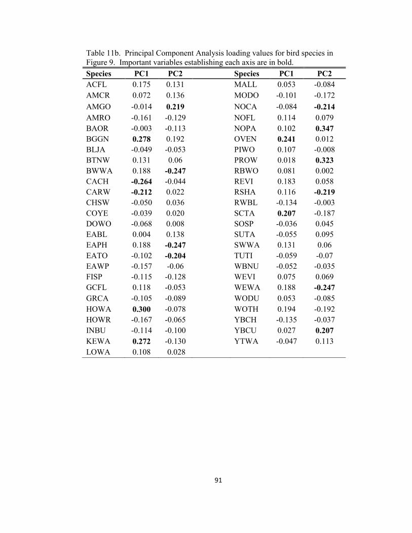
91
Table 11b. Principal Component Analysis loading values for bird species in
Figure 9. Important variables establishing each axis are in bold.
Species PC1 PC2 Species PC1 PC2
ACFL 0.175 0.131
MALL 0.053 -0.084
AMCR 0.072 0.136
MODO -0.101 -0.172
AMGO -0.014 0.219
NOCA -0.084 -0.214
AMRO -0.161 -0.129
NOFL 0.114 0.079
BAOR -0.003 -0.113
NOPA 0.102 0.347
BGGN 0.278 0.192
OVEN 0.241 0.012
BLJA -0.049 -0.053
PIWO 0.107 -0.008
BTNW 0.131 0.06
PROW 0.018 0.323
BWWA 0.188 -0.247
RBWO 0.081 0.002
CACH -0.264 -0.044
REVI 0.183 0.058
CARW -0.212 0.022
RSHA 0.116 -0.219
CHSW -0.050 0.036
RWBL -0.134 -0.003
COYE -0.039 0.020
SCTA 0.207 -0.187
DOWO -0.068 0.008
SOSP -0.036 0.045
EABL 0.004 0.138
SUTA -0.055 0.095
EAPH 0.188 -0.247
SWWA 0.131 0.06
EATO -0.102 -0.204
TUTI -0.059 -0.07
EAWP -0.157 -0.06
WBNU -0.052 -0.035
FISP -0.115 -0.128
WEVI 0.075 0.069
GCFL 0.118 -0.053
WEWA 0.188 -0.247
GRCA -0.105 -0.089
WODU 0.053 -0.085
HOWA 0.300 -0.078
WOTH 0.194 -0.192
HOWR -0.167 -0.065
YBCH -0.135 -0.037
INBU -0.114 -0.100
YBCU 0.027 0.207
KEWA 0.272 -0.130
YTWA -0.047 0.113
LOWA 0.108 0.028

92
Table 11c. Vector coefficients and goodness of fit statistics (R2) for habitat variables fit
to the KY-WRAM PCA in Figure 9 using Program R Package Vegan, function envfit.
Significant variables designated with a (*) indicate significance of P < 0.05, a (**)
indicate significance of P < 0.01, and a (***) indicate significance of P < 0.001.
Variable PC1 PC2 R2
forest 0.721 0.692 0.148
cult* -0.912 -0.409 0.273
k1 0.192 -0.981 0.033
k2** 0.990 0.134 0.581
k3 0.970 -0.244 0.114
k4** 0.982 -0.190 0.442
k5 0.832 -0.555 0.133
k6 0.949 0.316 0.052
fqai** 0.899 -0.437 0.482
shade*** 0.820 -0.572 0.519
st -0.542 0.841 0.159
subiv 0.981 -0.196 0.096
caniv -0.926 0.378 0.196
adv 0.954 -0.300 0.015

93
APPENDIX E
Supplemental Figures

94
Figure 7a. Linear regression between the VIBI score and LDI score. Different
symbols represent river basin for each site.
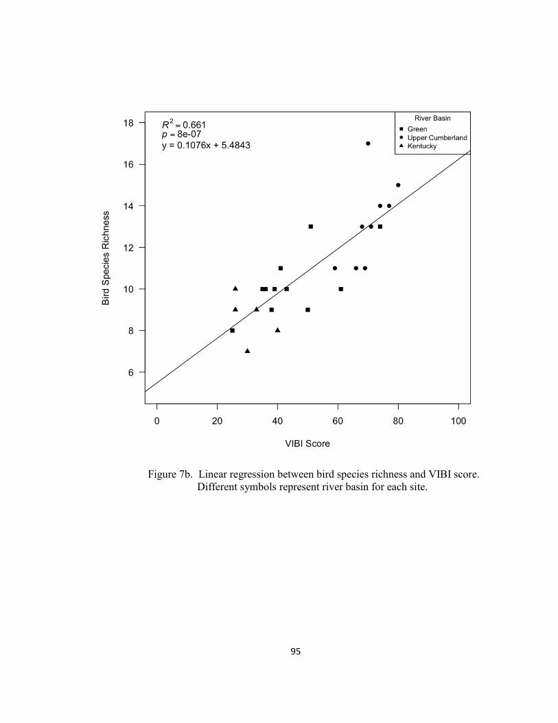
95
Figure 7b. Linear regression between bird species richness and VIBI score.
Different symbols represent river basin for each site.

96
Figure 7c. Linear regression between bird species richness and LDI score.
Different symbols represent river basin for each site.

97
Figure 8. Principal Component Analysis (PCA) of KY-WRAM metrics
across all sites. Vectors indicate increasing direction of change of
each metric. Red variables represent KY-WRAM metrics. Blue
variables represent an environmental fitting function of vegetation
metrics and landscape variables related to KY-WRAM metrics.
Numbers represent specific sites (see Table 2).

98
Figure 9. Principal Component Analysis (PCA) of bird species across all
sites. Vectors indicate increasing direction of change of each
species. Red variables represent bird species. Blue variables
represent an environmental fitting function of vegetation metrics,
KY-WRAM metrics, and landscape variables in relation to bird
species. Numbers represent specific sites (see Table 2).