validation of large structural dynamics models using modal test
TRANSCRIPT

IMPERIAL COLLEGE OF SCIENCE, TECHNOLOGY & MEDICINE
University of London
VALIDATION OF LARGE STRUCTURAL
DYNAMICS MODELS
USING MODAL TEST DATA
by
Nedzad Imamovic
A thesis submitted to the University of London
for the degree of Doctor of Philosophy
Department of Mechanical Engineering
Imperial College of Science, Technology & Medicine
London
February 1998
Abstract
This thesis presents research ideas and findings about structural dynamics modelvalidation when applied to real engineering problems. Since most practicalengineering problems involve modelling of complicated structures, the theoreticalmodels used are generally quite large and so this thesis focuses on application ofmodel validation to these large models.
Model validation consists of: data requirements, test planning, experimental testing,correlation, error location and updating. The goal of data requirements is to definethe required amount of experimental data for successful validation of a model. Thisrequirement for the optimum experimental data is coupled with test planning todesign an optimum modal test in terms of specifying the best suspension, excitationand response locations.
Test planning analysis uses the initial theoretical model (the model which is beingvalidated) and all new test planning methods are designed in such way that theyminimise the influence of any errors of the initial model to the results of testplanning.
Correlation is presented as a refined tool for automatic selection of correlated modepairs during updating, but correlation is also used for determination ofcompleteness of experimental data and determination of main discrepanciesbetween the two models.
Error location is studied extensively together with new practical limitations formodel updating parameters. No new updating method is introduced, but insteadthe existing sensitivity-based method is examined for its applicability to largeindustrial test cases. Particular attention is paid to automatic selection of updatingparameters during updating in order to keep the sensitivity matrix well-conditionedand to obtain an accurate solution for updating parameters.
Every test case presented in this thesis uses real experimental data rather thansimulated data and this gives a particular value of this work, as it is presented onseveral industrial applications throughout the text.

Acknowledgements
I would like to express my gratitude to my supervisor Prof. D J Ewins and to Dr. MImregun for their valuable advice, interest and encouragement throughout thisproject.
I would like to thank all my colleagues from Imperial College Dynamics Section forvaluable scientific discussions about the subject described in this thesis.
I am also grateful to Rolls-Royce plc. (particularly the Whole Engine ModellingGroup) for providing the financial and technical support for this project.
Special thanks are due to my parents, Resad and Alma and my brother Adem for alltheir love and support they provided during the course of this work, especiallyduring the last few months. Without them this thesis would not have beencompleted.

Nomenclature
Basic Terms, Dimensions and Subscripts
x,y,z translational degrees-of-freedom
N number of degrees-of-freedom of the complete theoretical model
n number of (measured) degrees-of-freedom of experimental model
s number of slave/secondary/unmeasured degrees-of-freedom
m number of modes of experimental model/
number of master degrees-of-freedom
ω , f frequency of vibration (in rads ;Hz respectively)
ε tolerance value
i, j,k,r integer indices
i −1
A, B,a,b real constants
Matrices, Vectors and Scalars
[ ] two dimensional matrix
{ } column vector
[‘ ‘] diagonal matrix
[ ]T transpose of a matrix
{ }T transpose of a vector
I[ ] identity matrix
[ ]−1 inverse of a matrix
[ ]+ generalised/pseudo inverse of a matrix
[ ]* complex conjugate of a matrix
U[ ], V[ ] matrices of left and right singular vectors
Σ[ ] rectangular matrix of singular values

S[ ] sensitivity matrix
T[ ] transformation matrix
norm of a matrix/vector
absolute value of a complex number
Spatial and Modelling Properties
M[ ] mass matrix
K[ ] stiffness matrix
D[ ] structural damping matrix
C[ ] viscous damping matrix
Modal and Frequency Response Properties
ω r natural frequency of r-th mode
ηr structural damping loss factor of r-th mode
mr generalised mass of r-th mode
kr generalised stiffness of r-th mode
[‘λ‘] eigenvalue matrix
ψ[ ] unit-normalised mode shape/eigenvector matrix
φ[ ] mass-normalised mode shape/eigenvector matrix
ψ{ }r; φ{ }
rr-th mode shape/eigenvector
α ω( )[ ] receptance matrix
Z ω( )[ ] dynamic stiffness matrix
α jk ω( )=x j
f k
individual element of receptance matrix between coordinates j and
k (response at DOF j due to excitation at DOF k)
r Ajk = φ jrφkr modal constant
R[ ] residual matrix

Standard Abbreviations
DOF(s) degree(s)-of-freedom
EMM error matrix method
FE finite element
FRF frequency response function
MAC modal assurance criterion
NCO normalised cross-orthogonality
SCO SEREP cross-orthogonality
COMAC coordinate modal assurance criterion
RFM response function method
SVD singular value decomposition
CMP(s) correlated mode pair(s)
ADPR Average Driving Point Residue
ADDOFD Average Driving DOF Displacement
ADDOFV Average Driving DOF Velocity
ADDOFA Average Driving DOF Acceleration
ODP Optimum Driving Point
NODP Non-Optimum Driving Point
EI Effective Independence

Structure of Thesis
Each chapter consists of several sections. Every section is numbered separatelyusing the chapter number to which the section belong followed by a separatenumber for section, such as 1.1, 3.4, etc. Some sections have further subsectionswhich have separate identification using section number followed by subsectionnumber such as 5.6.1, 7.2.5, etc.
All mathematical expressions (equations) in the text are numbered. Each expressionnumber consists of chapter, section and/or subsection number followed by theexpression number, such as 3-1, 4.2-3, 5.3.7-1, etc.
All figures given in the text also have a unique identification which is equivalent tothe numbering system for the equations. Majority of Figures are given within thetext, but some of them are given at the end of the relevant chapter.
For instance, if expression 4.3.2-6 is referenced somewhere in the text, then theadvantage of this numbering system is that the reader can instantly identify theposition of the equation in the text, in this case it is chapter 4, section 3 andsubsection 2. In most cases, the reader is given an opportunity to identify thementioned method by simply looking into the contents, or if it is necessary to find aparticular section then this numbering system gives an advantage.

Contents
Abstract
Acknowledgements
Nomenclature
Structure of Thesis
1.0 Introduction
1.1. Needs for Model Validation in Practice 1
1.2. Model Validation Definitions 4
1.3. Literature Survey 5
1.3.1. Test Planning 5
1.3.2. Correlation 6
1.3.3. Model Updating 7
1.4. Scope of the Thesis 9
1.5. Closing Remarks 10
2.0 Theoretical Modelling
2.1. Introduction 11
2.1.1. Analytical and Numerical Methods 11
2.1.2. Discrete Models and Concepts of Mass, Stiffness
and Damping 11
2.2. Numerical Modelling Analyses 12
2.2.1. Time-domain Analysis 12
2.2.2. Frequency-domain Analysis 14
2.2.3. Relationship between Time- and
Frequency-domain Analyses 14
2.3. Finite Element Method 15
2.3.1. Finite Element Mass and Stiffness Matrices Formulation 15

2.4. Governing Equation and Solution 17
2.4.1. Guyan (or Static) Reduction 19
2.4.2. Generalised Dynamic Reduction 20
2.4.3. SEREP Reduction 20
2.5. Eigensolution of Large Models 22
2.6. Conclusions 23
3.0 Planning of Modal Tests
3.1. Introduction 24
3.1.1. Pre-Test Planning 24
3.2. Signal Processing and Modal Analysis Mathematical Basics 25
3.3. Pre-Test Planning Mathematical Background 28
3.3.1. Time and Frequency Domains Relationship 28
3.3.2. Definitions for the Average Values
of Displacement, Velocity and Acceleration Amplitudes 30
3.4. Optimum Suspension Positions 32
3.4.1. Testing for Free-Free Boundary Conditions 32
3.5. Optimum Driving Positions 33
3.5.1. General Requirements for Optimum Excitation Positions 33
Process of Energy Transfer during Excitation 34
3.5.2. Hammer Excitation 35
3.5.3. Shaker Excitation 35
3.5.4. Optimum Driving Point (ODP) Technique 36
3.5.5. Non-Optimum Driving Point (NODP) Technique 36
3.5.6. Determination of the Optimum Driving Positions 37
ODP-Based Methods 38
NODP-Based Methods 38
3.5.7. Application of the ODP and NODP Techniques 39
Simple Plate 39
Engine Casing 48

3.5.8. Conclusions About Selection of Optimum
Suspension and Excitation Locations 52
3.6. Optimum Measurement Positions 52
3.6.1. Definitions for optimum measurement positions 53
3.6.2. Use of Average Displacement, Velocity and Acceleration 53
3.6.3. Effective Independence (EI) method 54
3.6.4. ADDOFV(A)-EI Method 55
3.6.5. Application of the EI and ADDOFV(A)-EI Methods 56
Clamped Disk 57
Simple Beam Structure
(Lloyd’s Register Correlation Benchmark) 59
Engine Nozzle Structure 61
3.6.6. Conclusions for Selection of Optimum
Measurement Locations 65
3.7. Reliability of Pre-Test Planning: Why/When does it work? 65
3.8. Closing Remarks 67
4.0 Model Correlation
4.1. Introduction 68
4.2. Standard Correlation Methods 68
4.2.1. Numerical Comparison of Mode Shapes 69
4.2.2. Visual Comparison of Mode Shapes 70
4.2.3. Problem of Complex Mode shapes 71
Assessing the Modal Complexity
of Experimental Mode Shapes 71
4.2.4. Realisation of Complex Mode Shapes 73
4.3. Reduction of Theoretical Model to the Number of Measured DOF 75
4.4. Minimum Test Data Requirements for Correlation 75
4.5. SEREP-based Normalised Cross
Orthogonality Correlation Technique 76
4.6. Natural Frequency Comparison 77
4.7. Automatic Correlation Procedure 78
4.8. Test Case Study 80
4.9. Comparison of Response Properties 83
4.10. Calculation of Frequency Response Functions (FRFs) 84
4.10.1. Finding The Residual Effects For
The System - The "Forest" Technique 87
4.11. "FOREST" Accuracy Diagram 91
4.11.1. Application Of The FOREST Technique 93
4.11.2. Application of the FOREST Accuracy Diagram 95
4.12. FOREST Test Case Study 95
4.13. Co-ordinate Modal Assurance Criterion (COMAC) 97
4.14. Conclusions 99
5.0 Error Location Theory
5.1. Introduction 100
5.1.1. Identification Approach 101
5.2. Causes of Discrepancies in Model Validation 102
5.2.1. Introduction 102
5.2.2. Errors in Experimental Data 104
5.2.3. Errors in Finite Element Modelling 104
Mesh Distortion Related Errors 105
Configuration Related Errors 107
5.3. Updating Parameters Definition 108
5.3.1. Whole Matrix Updating Parameter 108
5.3.2. Spatial-type Updating Parameter 109
5.3.3. Design-type Updating Parameter 110
5.3.4. General Spring-like Updating Parameter 110
5.3.5. Limitations of Updating Parameters Value 112
Singularity of the stiffness matrix 112
Ill-conditioning of the stiffness matrix 113

5.4. Selection of Updating Parameters 113
5.4.1. Classification of Methods for Initial
Selection of Updating Parameters 114
Empirically-based initial
selection of updating parameters 114
Sensitivity-based initial
selection of updating parameters 114
5.4.2. Important Factors in Selection of Updating Parameters 115
5.5. Objective Function Diagrams 116
5.5.1. Random Errors Distribution Theory 123
5.6. Conclusions 124
6.0 Model Updating
6.1. Introduction 125
6.1.1. Definition of The Updated Model 126
6.2. Classification of Updating Methods 127
6.2.1. Modal domain updating methods 127
6.2.2. Frequency domain updating methods 128
6.3. Application of Linear Regression Theory to Model Updating 128
6.3.1. Least-Squares Method 130
6.3.2. Singular Value Decomposition 133
6.3.3. Solutions of Overdetermined
and Undetermined Linear Systems 135
Solving of overdetermined updating equation 135
Normal equations 136
Solving of underdetermined updating equation 137
6.4. Assessment of the Rank and the Conditioning
of Updating Equation 138
6.4.1. Identifying the Column Space of the Matrix of Predictors 139
6.4.2. Selection of Updating Parameters using
Identifying the Column Space of the Matrix of Predictors 140
Use of cond S[ ]T S[ ]( ) for
selection of updating parameters 145
6.5. Calculation of Sensitivity Matrix 146
6.5.1. Calculation of Eigenvalue Sensitivities 146
6.5.2. Calculation of Eigenvector Sensitivities 146
6.5.3. Use of Eigenvector Sensitivities 148
6.5.4. Weighting of the Sensitivity Matrix (Updating Equation) 151
6.6. Conclusions 152
7. Model Validation Case Studies
7.1. Model Validation of Lloyd’s Register
Structural Dynamics Correlation Benchmark 153
7.1.1. Introduction 153
7.1.2. FE model 153
7.1.3. Experimental data 155
7.1.4. Correlation between experimental and initial FE results 155
7.1.5. Error localisation in FE model 156
7.1.6. Updating of FE model 156
7.1.7. Convergence of updating parameters 157
7.1.8. Correlation between experimental and updated FE model 159
7.1.9. Conclusions for Validation of
Lloyd’s Register Correlation Benchmark 160
7.2. Model Validation of an Aerospace Structure (C-Duct) 161
7.2.1. Introduction 161
7.2.2. FE model 161
7.2.3. Modal Test Data 161
7.2.4. Correlation between measured and the initial FE data sets 164
7.2.5. Error Localisation 166
7.2.6. Model Updating 167
7.2.7. Convergence of updating parameters 167
7.2.8. Selection of the final updated model 167
7.2.9. Conclusions for Validation of C-Duct
Structural Dynamic Model 170
8.0 Conclusions and Suggestions for Future Work
8.1. Conclusions 171
8.2. List of Contributions to Model Validation 175
8.2.1. Contributions to Test Planning 175
8.2.2. Contributions to Correlation 176
8.2.3. Contributions to Error Location Theory 176
8.2.4. Contributions to Model Updating 177
8.3. Suggestions for Future Work 177
8.6. Final Word 180
References 181
Appendices 197

MODEL VALIDATION OF LARGE FINITE ELEMENT MODELS USING TEST DATA, PhD ThesisNedzad Imamovic, Imperial College of Science, Technology & Medicine, London 1998
Chapter 1. Introduction__________________________________________________________________________________________
__________________________________________________________________________________________
Page 1
1. Introduction
This chapter provides a general introduction to structural dynamic model validationtechnology. Fundamental concept of model validation and its application in theoverall design process are outlined and some basic definitions for model validationtopics are introduced. In addition, a classification and comparison of existingvalidation techniques from different branches of mechanical engineering arepresented in this chapter. Finally, in the light of the application of model validationtechnology, the scope of this thesis is given at the end of the chapter.
1.1. Need for Model Validation in Practice
A traditional form of the "design-to-production-line" cycle of a product is shown inFigure 1.1. After the initial outline design of a product has been made, preliminaryanalysis including dynamic effects is performed and the first prototype is built.Various tests are carried out on the prototype, and if the prescribed properties of thedesign of the product are met, then full production can begin. However, it is veryunlikely that the initial design of a product will have all the previously-prescribeddesign properties and so some changes to the initial design become necessary. Afterthese changes are made, i.e. after the product has been re-designed, the wholevalidation process has to begin again, from analysis to building a new prototypeand testing. It can be seen that this route to final production might be veryexpensive and time-consuming, because in the case of any changes being made tothe initial design of the product, the whole process of building a new prototype totesting has to be repeated.
DESIGN ANALYSIS PROTOTYPE TEST PRODUCTION
RE-DESIGN
passed
failed
Figure 1.1. Simplified "Design-to-Production-Line" Cycle

MODEL VALIDATION OF LARGE FINITE ELEMENT MODELS USING TEST DATA, PhD ThesisNedzad Imamovic, Imperial College of Science, Technology & Medicine, London 1998
Chapter 1. Introduction__________________________________________________________________________________________
__________________________________________________________________________________________
Page 2
A more modern form of the "design-to-production-line" cycle is shown in Figure1.2. Here, after the initial design of the product, a preliminary analysis is performedand a prototype is built. Some "simple" non-destructive experiments, such as modaltests, may be performed on the prototype and the measured results compared withanalysis. This comparison between two data sets is known as the correlation
process. If the analytical predictions correlate (i.e. agree) well with the experimentalresults, then further analysis (aeroelasticity, transient dynamic, etc.) can beperformed using the same model. However, it is very unlikely that the initial modelof the structure will represent the measured behaviour accurately, and therefore itbecomes necessary to refine the initial model so that the predictions using therefined model are in acceptable agreement with the experimental results. Once arefined model which possesses the measured characteristics is found, it is possibleto simulate important verification tests that may be destructive and may requirecomplete or partial destruction of the prototype. This simulation of verification testsprovides a possibility of verifying the design without destruction of the prototype,and consequently the whole design and production process would have a lower costfor the manufacturer. If any of these simulated verification tests are not passed, thestructure undergoes a re-design process and the whole cycle is repeated from theprevious analysis step. Once the design specifications are met by a re-designedmodel, production can begin. It is clear that this route to the final product is cheaperthan the traditional way of design and verification since it does not require a newprototype after changes to the initial design.
To illustrate the above discussion, we shall compare these two design-and-verification approaches in the production of aircraft engines. When the first aircraftengine prototype is constructed, many design and working engine requirementshave to be verified. Some of these constraints are the containment, blade-off andbird-strike requirements at specific running conditions. These requirements arecrucial from the point of view of safety and every type of aircraft engine must betested in order to verify compliance with these requirements. These tests aredestructive and are consequently very expensive. However, if an accurate model ofthe structure is available, then it would be possible to simulate these tests fordifferent conditions, to predict engine behaviour during the events in question andto verify the design without destroying the whole engine every time one of thesetests is carried out. At this stage of development of model validation technology theresearch is concentrated on development of validation techniques which would

MODEL VALIDATION OF LARGE FINITE ELEMENT MODELS USING TEST DATA, PhD ThesisNedzad Imamovic, Imperial College of Science, Technology & Medicine, London 1998
Chapter 1. Introduction__________________________________________________________________________________________
__________________________________________________________________________________________
Page 3
enable engineers to carry out only one destructive test and to simulate other testswith different operating conditions, and therefore destroy only one engine insteadof several.
DESIGN ANALYSIS PROTOTYPESIMPLEEXPERIMENT
CORRELATION
UPDATING
FURTHERANALYSIS
TESTSIMULATION
RE-DESIGN
PRODUCTION
passed
passed
failed
failed
OPTIMUMTESTDESIGN
Figure 1.2. Simplified Modern “Design-to-Production-Line” Cycle.
Another example of the application of this technology is to aeroelasticity analysis,where the behaviour of coupled fluid-structure models is simulated in thecomputer. Although the predictions in fluid dynamic analysis are generally lessaccurate than those in structural dynamics, it is evident that having a verifiedstructural model would increase the accuracy of aeroelasticity predictions.

MODEL VALIDATION OF LARGE FINITE ELEMENT MODELS USING TEST DATA, PhD ThesisNedzad Imamovic, Imperial College of Science, Technology & Medicine, London 1998
Chapter 1. Introduction__________________________________________________________________________________________
__________________________________________________________________________________________
Page 4
1.2. Model Validation Definitions
The development of fast digital computers, numerical simulation techniques andmeasurement technology has led to an increase in the use of theoretical modelvalidation techniques in practice. Validation techniques combine the theoreticalsimulation of a phenomenon with experimental testing of an actual structure,leading to comparison and refinement of the theoretical model on the basis ofexperimental results. There are several scientific fields in which validationtechniques are used extensively, e.g. static-, stress-, fatigue-, fracture- and dynamicanalysis, but the fastest growing usage of validation techniques is in structuraldynamics. The reason for this rapid and extensive growth lies in the applicability ofvibration theory, well-established modal testing technology and well-developedmethods for numerical simulation of vibration phenomena whose theoreticalmodels can be used for other analysis. These reasons have contributed to a demandfor the development of a new area in structural dynamics analysis known asvalidation of structural dynamic models or, more commonly, model correlation
and updating.
Another important part of model validation process is test planning which hasemerged in the last few years as a precondition for successful correlation. Test
planning is a process of determining the optimum test parameters such assuspension, excitation and measurement locations on the basis of preliminarytheoretical predictions before commencement of the actual test. Clearly, the result oftest planning is dependent on the very model which is being validated and, as such,carries some uncertainties which have to be resolved during the validation process.This makes the test planning an extremely difficult problem since it relies on amodel which may have any degree of error and uncertainty.
Correlation is a process of comparison of the dynamic properties between two datasets. Although correlation is described as a comparison process, essentially it ismore than a simple comparison and in reality is also a process of assessment of theresult of test planning and the global completeness of experimental data set.

MODEL VALIDATION OF LARGE FINITE ELEMENT MODELS USING TEST DATA, PhD ThesisNedzad Imamovic, Imperial College of Science, Technology & Medicine, London 1998
Chapter 1. Introduction__________________________________________________________________________________________
__________________________________________________________________________________________
Page 5
There are many ways of defining model updating but the simplest and mostcommon definition is "adjustment of the theoretical model on the basis of modal testresults in order to minimise the discrepancies between theoretical and experimentalbehaviour of a structure" [1]. The advantages of an efficient model updating methodfor the simulation of structural behaviour are obvious, i.e. by performing only oneseries of modal tests on a structure, the initial model can be updated to match theexperimental results and this updated model can then be used for a wide range offurther dynamic analyses. Any results which come from further analysis need notbe validated since the model which was used to calculate those results was alreadyshown to be ’correct’. In practice, this means that once a successful updating of themodel of a structure is completed, there would be no need to perform and repeatexpensive experiments because the behaviour can be simulated theoretically usingthe updated model. Model validation can also be used to learn how to modelvarious structures, structural joints and other uncertainties in the modelling.
1.3. Literature Survey
This section gives a concise introduction to existing methods for model validationand it provides a list of the most important references. More details about somemethods described in this section can be found in relevant chapters and thereforeonly discussion about some existing methods is given here.
1.3.1. Test Planning
Test planning consists of determining the optimum suspension, optimum excitationand optimum response locations. Although each of these three requirements isequally important for a successful test, selection of optimum suspension is generallyviewed as being less significant than the other two requirements. Consequently, itappears that very little systematic research has been reported about selection ofoptimum suspension positions. Usually, the suspension for a modal test is selectedas such that there is least interference between the structure and the ground, and thedecision about suspension locations and orientation is based on the experience ofthe experimentalists. Some good tips about selection of suspension are described byEwins, [2].

MODEL VALIDATION OF LARGE FINITE ELEMENT MODELS USING TEST DATA, PhD ThesisNedzad Imamovic, Imperial College of Science, Technology & Medicine, London 1998
Chapter 1. Introduction__________________________________________________________________________________________
__________________________________________________________________________________________
Page 6
Selection of excitation location(s) is of paramount importance for a successful modaltest. There are two types of modal test as far as excitation strategy is concerned. Oneis the type where one reference point is used in the test to measure all modes withincertain frequency range, and in this case the reference point must be selected in aregion of structure where all modes are clearly recorded on the reference point FRF.An interesting study of this type of excitation was done by Lim, [3]. Another type ofmodal test is where multi-source of excitation is used for isolation of certain modes,usually when heavy damping is present in a structure. Some reference to thisparticular case of mode isolation can be found in [4].
Selection of measurement locations is critical for a successful modal test. There arenumerous instances where, after the test has been completed, it was concluded thateither an insufficient number of measurement locations was selected or too manypoints were measured and valuable time and resources were spent unnecessarily.One standard procedure for selection of measurement locations is to perform aGuyan reduction on the theoretical model and to select the same locations formeasurement as described in [5]. Another very efficient method was introduced byKammer which is based on estimation of the contribution of each observation to theleast-squares problem. The method is called Effective Independence and a fulldescription can be found in [6]. This method will be used (in this thesis) as a basisfor developing a new method for selecting optimum measurement locations.
1.3.2. Correlation
Correlation is probably the most mature area of model validation process. The mostfundamental form of correlation is a comparison between mode shapes using ModalAssurance Criterion (MAC) introduced by Allemang and Brown in [7]. A moreadvanced form of correlation based on the MAC formulation but using the mass orstiffness orthogonality property was introduced by Lieven in [8]. Modal Scale Factorwas introduced by Ewins, [2] and represents a measure of the slope between twomode shapes. The final result from this correlation is to produce a list of correlatedmode pairs (CMPs). It is important that each mode shape in a given data set islinearly independent of any other mode shape from the same data set. Clearly, thisrequirement is highly dependent on the choice of measurement locations and it isnecessary to evaluate the suitability of measurement locations. In most practicalcases, the MAC coefficient is used for this evaluation, but some other procedures

MODEL VALIDATION OF LARGE FINITE ELEMENT MODELS USING TEST DATA, PhD ThesisNedzad Imamovic, Imperial College of Science, Technology & Medicine, London 1998
Chapter 1. Introduction__________________________________________________________________________________________
__________________________________________________________________________________________
Page 7
can be successfully used, such as singular value decomposition (SVD), [9], or ameasure of the kinetic energy per mode, [10].
There are other forms of correlation, and another useful one is cross-orthogonalityfor every DOFs for selected number of modes. This procedure is known as Co-ordinate Modal Assurance Criterion and was introduced by Lieven and Ewins in[11].
1.3.3. Model Updating
Model updating is the most difficult part of the model validation process and as
such is the most challenging. Model updating is described as an area where most
effort was concentrated within structural dynamics community. Although recently
solving model updating problem in general is portrayed to have a similar fate as
general solution of model identification problem, still model updating as a primary
part of model validation process has its established role.
One of the major problems in model updating is incompleteness of experimental
model in terms of the number of measured DOFs. This problem has been overcome
in some situations either by reducing the theoretical (usually the larger data set)
model or by expanding the experimental model, although the author came across a
few practical cases in which experimental data set had larger number of DOF
thanks to laser scanning techniques applied in modal testing. Several reduction and
expansion techniques can be found in [12],[13],[14],[5] and [15].
Model updating methods can be classified in two groups as far as the data used for
updating is concerned. One group includes methods which use direct frequency
response data for updating, and the other group contains methods which use modal
data. Methods which use modal data for updating can be further divided into two
groups; (i) direct methods and (ii) iterative methods.

MODEL VALIDATION OF LARGE FINITE ELEMENT MODELS USING TEST DATA, PhD ThesisNedzad Imamovic, Imperial College of Science, Technology & Medicine, London 1998
Chapter 1. Introduction__________________________________________________________________________________________
__________________________________________________________________________________________
Page 8
One of the most simple direct updating approaches is Error Matrix Method (EMM)proposed by Sidhu and Ewins [16]. The method proposed earlier by Baruch[17]assumes that the mass matrix is correct and updated the stiffness matrix usingLagrange multipliers. The problem with these methods is that they correct eithermass or stiffness matrix globally, usually ruining the sparseness of the systemmatrices which is unacceptable for large models.
Methods based on force balance assume that mass matrix is accurate and theycorrect the stiffness matrix using the force balance equation as describes by Berger,Chaquin and Ohayon [18]. Link [19],[20] used this approach to develop a newmethod for model updating by minimising the force residue using a weighted least-squares approach. Also, methods based on orthogonality were proposed by Niedbal[21] to solve the updating problem, usually as a least-squares approach. Manydifferent variations of the force balance and orthogonality methods have beenproposed, but their major weakness is that they require full experimental modeshape vectors and as such they are not directly applicable for updating of largemodels because their use would require either reduction of larger model orexpansion of smaller model.
The sensitivity method [22],[23] is a prime representative of the updating approachwhich allows selection of updating parameters but does not require fullexperimental mode shapes and as such this method seems to be suitable forupdating of large models. Also, it is worth noting that model updating methodsbased on control methods, such as eigenstructure assignment method proposed byMinas and Inman [24],[25] are quite promising since they can be defined in such away that they do not require full experimental mode shape matrix.
Lin and Ewins [26] proposed a method which uses frequency response data forupdating of structural models instead of modal data. There is another family ofmethods which use frequency response data directly, such as method ofminimisation of response equation errors proposed by Natke [1]. Again, there areseveral variations of this updating approach, and most of them allow selection ofupdating parameters and can cope with incompleteness of experimental data quitewell. A major shortcoming of these methods is that they usually do not lead to aproper least-squares approach due to the presence of noise in the experimental data,as will be explained in more detail in chapter 6.

MODEL VALIDATION OF LARGE FINITE ELEMENT MODELS USING TEST DATA, PhD ThesisNedzad Imamovic, Imperial College of Science, Technology & Medicine, London 1998
Chapter 1. Introduction__________________________________________________________________________________________
__________________________________________________________________________________________
Page 9
There is a new family of updating approaches based on stochastic optimisationmethods such as the genetic algorithm (GE) method. Genetic algorithms are mainlyused for solving complicated optimisation problems and they have the advantageover deterministic optimisation approaches, such as simulated annealing (SA), thatthey provide faster convergence to near global minimum value. These two methods(GA and SA) seem to be very promising, but at this stage their contribution tomodel updating is more of an academic character and they are still not ready forapplication to large models.
1.4. Scope of the Thesis
Model validation has reached a critical stage when it is rapidly becoming anessential tool in the design process. There is no doubt that the aerospace industry isbecoming a major user of model validation technology. At this stage, many differentupdating methods were developed, and many researchers rushed to produce yetanother different method for model updating, which works well on simulated casestudies but often fails to produce good results when used with real experimentaldata.
In order to apply model validation technology to real engineering problems, it isnecessary to close the gaps between the test planning, correlation and updatingprocesses. These three processes have to be integrated with the requirementsdescribed for the final updated model so that a model validation strategy can bedefined which can offer solutions for real engineering problems.
In order to reach these goals the following needs to be done and forms the basis ofresearch in this thesis:
(i) It is necessary to define the minimum data requirements for correlation andupdating using the information about the final application of the models to bevalidated;
(ii) development of methods which will enable the user to plan a modal test usingany available preliminary knowledge about the model. Test planning has to be usedto ensure that the minimum effort is spent obtaining the most valuable informationabout the structure’s dynamic behaviour;

MODEL VALIDATION OF LARGE FINITE ELEMENT MODELS USING TEST DATA, PhD ThesisNedzad Imamovic, Imperial College of Science, Technology & Medicine, London 1998
Chapter 1. Introduction__________________________________________________________________________________________
__________________________________________________________________________________________
Page 10
(iii) a comprehensive study of error location theory is required;
(iv) experience suggests that currently the most promising numerical updatingapproach is the sensitivity method and therefore this method has to be adapted forapplication to large theoretical models;
(v) an additional constraint for this study is that any new method has to be testedand verified using practical experimental data. There seems to be too manyacademically valuable algorithms which work successfully only when simulatedexperimental data is used.
These tasks constitute the work reported in this thesis which is structured as follow:Chapter 2 provides theoretical background information about vibration theory andfinite element modelling technology. Chapter 3 gives details about test planning.Chapter 4 describes the correlation process and defines a new automatic correlationprocedure to be used in updating. Chapter 5 provides a comprehensive study abouterror location in finite element models. Chapter 6 gives detailed analysis aboutlimitations of the sensitivity least-squares updating approach. Chapter 7 givesdetails about two practical model validation test cases. Chapter 8 presents someoverall conclusions and provides a list of specific contributions made in this projectand suggestions for further research.
1.5. Closing Remarks
It is the author’s belief that recognising and identifying the role of model validationin the overall design process is an important process that should be well understoodbefore attempting a systematic study of model validation such as this. Positions androles of model validation technology within the design process are clearly identifiedand highlighted in this chapter.

MODEL VALIDATION OF LARGE FINITE ELEMENT MODELS USING TEST DATA, PhD ThesisNedzad Imamovic, Imperial College of Science, Technology & Medicine, London 1998
Chapter 2. Theoretical Modelling__________________________________________________________________________________________
______________________________________________________________________________________
Page 11
2.0 Theoretical Modelling
2.1. Introduction
This chapter provides an introduction to the basis of theoretical modelling used in
model validation technology.
2.1.1. Analytical and Numerical Methods
Theoretical prediction techniques used in structural dynamics can be divided into
two main families: one based on classical analytical methods and the other on
numerical methods.
Classical analytical methods are restricted to simple types of structure (one- and
two-dimensional structures of simple geometric form) because they do not discretise
the structural domain but the solution is found continuously for the whole domain.
Numerical methods approximate and divide the solution domain and find a
solution for a certain number of discrete points throughout the domain. Numerical
methods are applicable to structures of arbitrary geometry and these methods will
be used to predict and validate the dynamic behaviour of structures in this work.
2.1.2. Discrete Models and Concepts of Mass, Stiffness and Damping
A discrete model of a structure consists of elements that are defined by several
nodes. Adjacent elements are connected through common nodes to form an
assembled discrete model of the structure. Each element is defined by its nodes,
material and physical properties, and these data are used for defining mass,
stiffness and damping matrices of the element. Each node has six degrees-of-
freedom, three translations and three rotations.
The mass matrix of an element is a basic representation of its inertia properties
concentrated at degrees-of-freedom at nodes which define the element.
MODEL VALIDATION OF LARGE FINITE ELEMENT MODELS USING TEST DATA, PhD ThesisNedzad Imamovic, Imperial College of Science, Technology & Medicine, London 1998
Chapter 2. Theoretical Modelling__________________________________________________________________________________________
______________________________________________________________________________________
Page 12
The stiffness matrix of an element provides information about stiffness properties at
degrees-of-freedom at nodes which define the element.
The damping matrix of an element defines damping properties at degrees-of-freedom at nodes which define the element.
Thus, using simple concepts of mass, stiffness and damping formulations, anystructure can be represented at a number of nodes. The sum of all degrees-of-freedom at all defined nodes of a model is called the total number of degrees-of-freedom and this number is an important characteristic of the model. The totalnumber of degrees-of-freedom can vary for different models, but experience showsthat for accurate predictions of the dynamic properties of practical structures thisnumber can be quite large. It is quite common to come across models which haveseveral hundred thousand degrees-of-freedom and these models can be somewhatdifficult to analyse because of their size. This work is particularly focused on theapplication of model validation techniques for these large models. The term ‘largemodel’ is explained in section 2.5.
2.2. Numerical Modelling Analyses
Numerical prediction methods can be implemented in either the time or thefrequency domains.
2.2.1. Time-domain Analysis
Time-domain predictions (transient analysis) are the most general and can dealwith any type of excitation pattern or structural non-linearity (geometrical, material,etc.), but the calculations are expensive and CPU time-consuming. The disadvantageof time-domain analysis is the difficulty in performing the equivalent experiment,and the repeatability, impracticality and cost of transient experiments. Furthermore,transient analysis can be performed as either direct or segregated. A direct
transient analysis generates and assembles the full structural matrices and solves allunknowns at every time step (e.g. the Finite Element Method), while the segregated
transient analysis partitions the solution equations into several sets of unknownsinstead and solves each unknown set separately, using the last values of theunknowns when solving for a new unknown set until all unknowns converge tostable solution values (e.g. the Finite Volume and Boundary Element Methods).

MODEL VALIDATION OF LARGE FINITE ELEMENT MODELS USING TEST DATA, PhD ThesisNedzad Imamovic, Imperial College of Science, Technology & Medicine, London 1998
Chapter 2. Theoretical Modelling__________________________________________________________________________________________
______________________________________________________________________________________
Page 13
Also, a transient analysis requires the modelling of the damping and the solutiontends to be very dependent on the damping model used, which is generallyunknown and difficult to specify.
A general limitation of the transient type of analysis is the incremental time stepused, ∆tmin . Usually, in order to obtain convergence in a transient analysis, the time
step is determined by consideration of wave propagation and the size of the mesh. Itis common practice to set the time step to a value small enough such that the wavescan be ‘caught’ between the two nearest nodes several times before the changetransfers from one node to the other. If the distance between any two adjacent nodesin the mesh is ∆Xmin , and the maximum wave velocity in the material domain iscwave , then the maximum allowed transient analysis time step ∆tmax is defined by the
following expression:
∆tmax =∆Xmin
cwave
(2.2.1-1)
The actual transient analysis time step must be smaller than this maximum allowedvalue but too small a value would require a huge CPU effort and would beimpractical, i.e.:
ATHRESHOLD<<∆tmin <∆tmax (2.2.1-2)
where ATHRESHOLD is the computer threshold value. The time step used must be
significantly larger than the threshold value, which is dependent on the number ofdigits that the computer can store for one number. The threshold value is defined asthe minimum value of variable ε for which the expression below holds:
ATHRESHOLD = min(ε) such that a + ε > a, a ∈ R. (2.2.1-3)
For double-precision representation of real numbers (each real number isrepresented by 16 digits only), the threshold value obtained by applying the abovealgorithm is
ATHRESHOLD(16 −digits ) = 2.2204460492503130 x 10⁻¹⁶ (2.2.1-4)
MODEL VALIDATION OF LARGE FINITE ELEMENT MODELS USING TEST DATA, PhD ThesisNedzad Imamovic, Imperial College of Science, Technology & Medicine, London 1998
Chapter 2. Theoretical Modelling__________________________________________________________________________________________
______________________________________________________________________________________
Page 14
while for single-precision real number the threshold value is
ATHRESHOLD(8− digits) = 1.1920929 x10 −7 (2.2.1-5)
The threshold coefficient value is an important parameter that will be used
throughout this text and constitutes a general limitation of the application of
numerical methods.
2.2.2. Frequency-domain Analysis
The frequency-domain method of analysis has a major advantage in the practicality
of vibration theory, namely: repeatable and cheap numerical analysis. The main
disadvantage of numerical analysis in the frequency domain is the difficulty of
modelling material and geometrical non-linearities and of other types of non-
linearity. From the computational point of view, this type of analysis is not
particularly CPU-time expensive but does require a large amount of active (RAM)
memory. Frequency-domain analysis does not necessarily require modelling of
damping in the model, which further simplifies the analysis and makes the
computational effort more realistic and affordable. The main limitation of frequencydomain analysis is the maximum frequency value, f max , above which the natural
frequencies and mode shapes cannot be extracted from the spatial model. Generally,
it is not possible to calculate all the natural frequencies and mode shapes from an FE
model and only a limited number of them would be accurate, even if convergence is
obtained, as the higher mode shapes would resemble noise. Another limitation, as
far as the upper value of the frequency range of interest is concerned, is the time-
sampling of the measured signal in order to measure the higher frequency
responses.
2.2.3. Relationship between Time- and Frequency-domain Analyses
After obtaining a solution in the time domain, it is possible to convert the results
into the frequency domain. This transformation is based on Fourier Analysis and
will be described in more detail in section 3.2. It is, however, appropriate to give
here the relationship between the limits of the transient, ∆tmin , and the frequency,f max , analyses. If the structural model has been validated in a frequency range
MODEL VALIDATION OF LARGE FINITE ELEMENT MODELS USING TEST DATA, PhD ThesisNedzad Imamovic, Imperial College of Science, Technology & Medicine, London 1998
Chapter 2. Theoretical Modelling__________________________________________________________________________________________
______________________________________________________________________________________
Page 15
whose upper limit is f max , then the minimum transient analysis time step which
should be used is defined by the following expression:
∆tmin =C
f max
. (2.2.3-1)
The constant C takes a value typically in the range 5-10 in order to ensure that onlythose modes which belong to the validated frequency range contribute to thetransient analysis. It will be shown later that the contribution of each mode to thetotal response is inversely proportional to the square of the natural frequency of thatmode. Since the higher modes have larger natural frequencies, their contribution tothe total response decreases with increasing mode number.
Numerical example of corresponding limits in the time and frequency domain:f 2 = 500 Hz
C = 5∆tmin = 0.01 sec
The above example shows that if the structural model has been validated up to thelimiting frequency, f max , then any transient analysis with a time step value greater
than ∆tmin should give a time history result that is accurate up to a level which is
determined by the maximum contribution of the first omitted mode inside thevalidated frequency range.
2.3. Finite Element Method
The most commonly-used modelling technique for prediction of the dynamicproperties of structures (natural frequencies and mode shapes) and of their responsecharacteristics is that of Finite Element Analysis [27],[28],[29],[30],[31]. The FiniteElement Method is based on discretisation of the structural geometry domain intoseparate elements which are used to create global mass, stiffness and dampingmatrices.
2.3.1. Finite Element Mass and Stiffness Matrices Formulation
The Finite Element Method is based on discretisation of the structural domain intoseparate elements for which shape functions are defined and each element is

MODEL VALIDATION OF LARGE FINITE ELEMENT MODELS USING TEST DATA, PhD ThesisNedzad Imamovic, Imperial College of Science, Technology & Medicine, London 1998
Chapter 2. Theoretical Modelling__________________________________________________________________________________________
______________________________________________________________________________________
Page 16
constructed from several nodes. The stiffness matrix of a finite element is definedusing the principle of minimum potential energy. If a finite element consists of r
nodes, then the co-ordinates, x , and the displacements, u , of interior points can beexpressed in terms of the co-ordinates, xi , and the displacements, ui , at those nodes,
as follows:
x = Nixii =1
r
∑ (2.3.1-1)
u = Niuii =1
r
∑ (2.3.1-2)
The general formulation of the structural mass and stiffness matrices, when theshape functions are defined in the local co-ordinate system, is as follows:
Me[ ]= N[ ]T ρ N[ ]det J( )dξ1dξ2dξ3
−1
1
∫−1
1
∫−1
1
∫ (2.3.1-3)
Ke[ ]= B[ ]TD[ ] B[ ]det J( )dξ1dξ2dξ3
−1
1
∫−1
1
∫−1
1
∫ (2.3.1-4)
where N[ ] is the shape function matrix,B[ ] is the derivative of the shape function matrix,D[ ] is the matrix of material constants ,J[ ] is the Jacobian matrix between the global and a local element co-ordinate
system.
As can be seen from expressions (2.3.1-3) and (2.3.1-4), the terms in the structuralmass and stiffness matrices are not explicit functions of the finite element designparameters such as node positions, material properties, area, second moment of areaand physical dimensions of the structure. In order to obtain the values of the massand stiffness matrix terms, integration is required over the domain of the singleelement. Unfortunately, it is not possible to solve the integrals in the expressions(2.3.1-3) and (2.3.1-4) analytically; only a numerical solution can be found, whichfurther complicates the function between mass and stiffness matrix elements and thefinite element design parameters.

MODEL VALIDATION OF LARGE FINITE ELEMENT MODELS USING TEST DATA, PhD ThesisNedzad Imamovic, Imperial College of Science, Technology & Medicine, London 1998
Chapter 2. Theoretical Modelling__________________________________________________________________________________________
______________________________________________________________________________________
Page 17
The overall mass and stiffness matrices are obtained by assembling mass andstiffness matrices of the individual elements at the common nodes and are definedby the following expressions:
MA[ ]= Me[ ]i =1
Nelem
∑ (2.3.2-5)
KA[ ]= Ke[ ]i=1
Nelem
∑ (2.3.2-6)
The mass matrix formulation using expression (2.3.1-3) gives a so-called ‘consistent’mass matrix and predictions using this formulation are usually more accurate thanpredictions using a lumped mass matrix formulation. The lumped mass matrixformulation is a simple concentration of the mass at the translational degrees-of-freedom; this leads to a diagonal form of mass matrix.
Unfortunately, it is not possible to derive an expression that would define adamping matrix for a general structural element, such as the mass or stiffnessmatrix expressions given in (2.3.1-3) and (2.3.1-4). In practice, a global dampingmatrix is assembled from damping values between several pairs of degrees-of-freedom, and these damping values are simply specified by the analyst. A dampingcoefficient between two degrees-of-freedom cannot be derived from the physicalproperties of elements and these parameters are extremely complex to modelaccurately.
2.4. Governing Equation and Solution
The equation of motion for a structural system which has N degrees-of-freedom,and considering general viscous damping, is of the following form:
MA[ ] Ý Ý x { }+ CA[ ] Ý x { }+ KA[ ] x{ }= f{ } (2.4-1)
Since it is very difficult to model damping accurately, different forms of damping(e.g. proportional damping) can be assumed in order to simplify the analysis, but inmost cases damping can be excluded when natural frequencies and mode shapesare calculated so that the following equation is obtained:
MODEL VALIDATION OF LARGE FINITE ELEMENT MODELS USING TEST DATA, PhD ThesisNedzad Imamovic, Imperial College of Science, Technology & Medicine, London 1998
Chapter 2. Theoretical Modelling__________________________________________________________________________________________
______________________________________________________________________________________
Page 18
MA[ ] Ý Ý x { }+ KA[ ] x{ } = f{ } (2.4-2)
Considering the homogeneous part of the expression (2.4-2) and assuming aharmonic response of the following form:
x t( ){ }= φ{ }eiωt (2.4-3)
the generalised form of the eigenproblem can be written in the form
KA[ ]− ω 2 MA[ ]( ) φ{ }= 0{ } (2.4-4)
where natural frequencies are defined by solution of the following expression
det KA[ ]− ω2 MA[ ]( )= 0 (2.4-5)
The solution of the equation (2.4-5) leads to N values of the natural frequency,ω1, ..ωr .,ω N , which can be substituted back into equation (2.4-4) to yield the modeshapes φ1{ }, ..., φN{ } (also called normal modes), which describe the deformation
shapes of the structure when it vibrates at each of the corresponding naturalfrequencies.
By performing a simple algebraic manipulation, it can be shown that the mass-normalised mode shapes satisfy the orthogonality conditions with respect to massand stiffness matrices as defined in the following expressions:
φ[ ]TM[ ] φ[ ]= \I\[ ] (2.4-6)
φ[ ]TK[ ] φ[ ]= \ω r
2\[ ] (2.4-7)
Later, it will be seen that the orthogonality conditions are important features ofmode shapes for both correlation and updating.
The basic equation (2.4-2) may need reduction prior to solution in the case of nullcolumn appearance in a mass matrix. These massless degrees-of-freedom can beeffectively removed using static (i.e. Guyan) reduction without altering the finalsolution. In the case of having too large a model there are other reductions which

MODEL VALIDATION OF LARGE FINITE ELEMENT MODELS USING TEST DATA, PhD ThesisNedzad Imamovic, Imperial College of Science, Technology & Medicine, London 1998
Chapter 2. Theoretical Modelling__________________________________________________________________________________________
______________________________________________________________________________________
Page 19
can be applied in order to make the solution of expression (2.4-5) possible, but anyreduction of the full set (apart from the massless degrees-of-freedom) would alterthe calculated dynamic properties of the system. The most common reductiontechniques are: (i) Static (Guyan) reduction, (ii) Generalised Dynamic reduction, and(iii) SEREP reduction. These reduction techniques are described in detail in thefollowing sections.
2.4.1. Guyan (or Static) Reduction
The Guyan [5] or Static reduction technique is a simple approach which has theparticular feature of removing massless degrees-of-freedom without altering thefinal solution of the eigenproblem described in expression (2.4-4). The mass andstiffness matrices of the full model are partitioned into master and slave degrees-of-freedom, as indicated in the following expression:
Mmm Mms
Msm Mss
Ý Ý x mÝ Ý x s
+Kmm Kms
Ksm Kss
xm
xs
=0
0
(2.4.1-1)
Neglecting the inertia terms for the second set of equations, and after expressing thexs set of co-ordinates as functions of stiffness terms, the following transformation
matrix is obtained:
xm
xs
=I
−Kss−1Ksm
xm{ }= Ts[ ] xm{ } (2.4.1-2)
The Guyan-reduced mass and stiffness matrices are then defined as
MR[ ]= Ts[ ]TM[ ] Ts[ ] and (2.4.1-3)
KR[ ]= Ts[ ]TK[ ] Ts[ ], respectively. (2.4.1-4)
In the case of removing non-massless degrees-of-freedom, this reduction techniquewill produce an exact response only at zero frequency.

MODEL VALIDATION OF LARGE FINITE ELEMENT MODELS USING TEST DATA, PhD ThesisNedzad Imamovic, Imperial College of Science, Technology & Medicine, London 1998
Chapter 2. Theoretical Modelling__________________________________________________________________________________________
______________________________________________________________________________________
Page 20
2.4.2. Generalised Dynamic Reduction
The previous section describes how to reduce system matrices by neglecting theinertia terms from expression (2.4.1-1). If, however, the inertia terms are notneglected when expressing slave co-ordinates as a function of master co-ordinates,then the following transformation matrix can be obtained:
xm
xs
=I
− Kss − ω 2Mss( )−1Ksm − ω 2Msm( )
xm{ }= TD[ ] xm{ } (2.4.2-1)
This method is an extension of the Guyan reduction process in that the responseproperties are equivalent to those of the full matrices only for the frequency thatwas specified in the reduction process [14]. The transformation matrix is used in thesame way as specified in expressions (2.4.1-3) and (2.4.1-4) to obtain reduced systemmatrices.
2.4.3. SEREP Reduction
Most reduction processes reduce the size of the model but do not generally retainthe properties of the initial model, expect in the SEREP reduction process, [14]. Thisprocess reduces the size of the original model while retaining the exact modalproperties and is not dependent on the choice of master co-ordinates [56].
The SEREP transformation can be written as follows
X{ }N = φ[ ]NxmP{ }m (2.4.3-1)
We can rewrite equation (2.4.3-1) with respect to the master and slave degrees offreedom, Xn and Xs , respectively as:
Xn
Xs
=φn
φ s
Nxm
P{ }m (2.4.3-2)
where n is the number of measured co-ordinates and m is the number of measuredmodes.

MODEL VALIDATION OF LARGE FINITE ELEMENT MODELS USING TEST DATA, PhD ThesisNedzad Imamovic, Imperial College of Science, Technology & Medicine, London 1998
Chapter 2. Theoretical Modelling__________________________________________________________________________________________
______________________________________________________________________________________
Page 21
From equation (2.4.3-2), the vector of displacements in the master co-ordinates is
X{ }n = φ[ ]nxmP{ }m (2.4.3-3)
Using equation (2.4.3-3), it is possible to determine the displacement vector inmodal co-ordinates as follows:
P{ }m = φ[ ]mxn
+X{ }n (2.4.3-4)
where φ[ ]mxn
+ denotes the pseudo-inverse of φ[ ]nxm. In order to have a unique
solution of the least-squares problem in equation (2.4.3-4), the following conditionmust be satisfied [9]:
rank( φ[ ]nxm) = m (2.4.3-5)
and this means that a required condition is that n ≥ m , i.e. the number ofmeasurement co-ordinates must be greater than or equal to the number of measuredmodes. However, the condition n ≥ m is not sufficient, even if there are more co-ordinates than modes, as the rank may or may not be equal to the number of modes.The rank of the measured mode shape matrix depends on the choice of themeasured co-ordinates as well as their number. For example, if five modes havebeen extracted by measuring ten degrees-of-freedom all near the tip of a cantileverbeam, the φ[ ]nxm
matrix will almost certainly be rank-deficient. This requirement
will be used later in order to determine the minimum data requirements forcorrelation.
In order to satisfy condition (2.4.3-5), the relation between the full set of co-ordinates and the master co-ordinates is:
X{ }N = T[ ]Nxn X{ }n (2.4.3-6)
where the transformation matrix, T[ ], is given by:
T[ ]Nxn = φ[ ]Nxmφ[ ]mxn
+ (2.4.3-7)

MODEL VALIDATION OF LARGE FINITE ELEMENT MODELS USING TEST DATA, PhD ThesisNedzad Imamovic, Imperial College of Science, Technology & Medicine, London 1998
Chapter 2. Theoretical Modelling__________________________________________________________________________________________
______________________________________________________________________________________
Page 22
Reduced mass and stiffness system matrices are given by:
MR[ ]nxn= T[ ]nxN
TM[ ]NxN T[ ]Nxn (2.4.3-8)
KR[ ]nxn= T[ ]nxN
TK[ ]NxN T[ ]Nxn (2.4.3-9)
After substituting equation (2.4.3-7) into equations (2.4.3-8) and (2.4.3-9), thereduced mass and stiffness matrices become
MR[ ]nxn= φ[ ]nxm
+T φ[ ]mxn
+ (2.4.3-10)
KR[ ]nxn= φ[ ]nxm
+T \ω \2[ ]
mxmφ[ ]mxn
+ (2.4.3-11)
For more details of the properties of these matrices, see reference [56].
2.5. Eigensolution of Large Models
Most engineering structures are quite complicated and consequently their finiteelement models are also complicated and large. The description ‘large’ applied to afinite element model is a relative one and cannot be precisely defined. Usually,‘large’ is defined by the size of the RAM and ROM memory of the computer used.Model validation technology application almost certainly requires several iterationsto be performed, but there is no guarantee that an accurate model will be foundafter analysis and therefore nobody will invest an excessive amount of money forapplication of this technology. Also, there are some methods in model validationtechnology that require a large amount of memory, such as the calculation ofeigenvector sensitivities, and there are physical limitations imposed by the availablefacilities on the size of the largest finite element model. In addition, modelvalidation methods involve complex calculations of matrices whose sizes aredetermined from the total number of degrees-of-freedom of the finite elementmodel, and special care has to be taken to ensure that some practically-impossiblecriteria are not generated by use of improper numerical methods.

MODEL VALIDATION OF LARGE FINITE ELEMENT MODELS USING TEST DATA, PhD ThesisNedzad Imamovic, Imperial College of Science, Technology & Medicine, London 1998
Chapter 2. Theoretical Modelling__________________________________________________________________________________________
______________________________________________________________________________________
Page 23
What, then, does the term ‘large finite element model’ mean here?A simple answer to this question is that the word ‘large’ is not associated with aparticular number. The use of the term ‘large’ finite element model means that thesemethods obviate the need for some conditions or calculations which may beimpossible in practical terms. One good example of these practically unattainableconditions is one which requires calculation of all mode shapes of a finite elementmodel of a structure in order to eliminate the residual effects on the FrequencyResponse Functions. Even though this task could be performed for some modelsprovided that available facilities do not impose limits, in most practical situationsthere is no method that would offer an accurate solution for the calculation of thehigher mode shapes.
2.6. Conclusions
Numerical modelling techniques, and the Finite Element Method in particular, areultimately tools for prediction of the dynamic behaviour of structures. The time-domain method of analysis is the most general but is computationally veryexpensive, while the frequency-domain analysis is not as generally applicable forsimulation but is computationally less expensive and as such it has a place as aprimary validation type of analysis. Most simulation techniques are based on time-domain analysis methods, but the equivalent experiments are very expensive andinappropriate for model validation. The relationship between the limitations of thetime- and frequency-domain analyses gives a clear starting point for defininggeneral data requirements for validation of structural dynamic models. Afterdefining further analysis of a structural dynamic model, the analyst can define theminimum transient analysis time step for the further analysis, and this informationcan be used for determination of the frequency range in which the structural modelhas to be validated. This frequency range is a base for determination of theminimum data requirements for model validation, as will be pointed out in thefollowing chapters.
MODEL VALIDATION OF LARGE FINITE ELEMENT MODELS USING TEST DATA, PhD ThesisNedzad Imamovic, Imperial College of Science, Technology & Medicine, London 1998
Chapter 3. Planning of Modal Tests__________________________________________________________________________________________
______________________________________________________________________________________
Page 24
3.0 Planning of Modal Tests
3.1. Introduction
Modal testing is one of the fastest-growing experimental techniques of the last twodecades. There are a number of different industrial sectors which use modal testingas a standard link in the production chain. Modal testing is a method of constructinga mathematical model of the structure’s dynamic behaviour based on vibration testdata rather than on a theoretical analysis of the structure.
Although the mathematical basis of modal testing is well developed, experienceshows that the quality of results obtained by applying modal testing can be sensitiveto the set-up of experiments. There are some elements of these experiments that arenot easy to incorporate in modal testing but, fundamentally, they are an importantpart of it. These elements are normally assumed to be perfect in the theory of modaltesting, and are: (i) suspension of the test piece, (ii) choice of driving positions and(iii) choice of measurement positions. This chapter provides a theoretical basis thatcan be applied to determine the optimum suspension, driving and measurementpositions or, more precisely, to plan optimum modal tests.
3.1.1. Pre-Test Planning
Each time a modal test is undertaken on a structure, one of the first things which hasto be decided is how many and which responses should be measured, how thestructure should be suspended and which positions are most suitable as excitationlocations. Usually, experience and intuition are used to answer these questions, butin many cases, after the test is finished and when reviewing the experimental results,it is realised that not all the best measurement points were always selected or maybethat some of them need not have been measured at all, and the same applies tosuspension and excitation position.
One of the approaches used to select measurement points is to show visually apreliminary estimate of the theoretical mode shapes and the corresponding naturalfrequencies of the structure and, on the basis of these data, to select the optimumsuspension, excitation and measurement positions. This is not a strongly-recommended approach since any prior knowledge of the values for modalparameters of a theoretical model can influence measurements and, in extreme
MODEL VALIDATION OF LARGE FINITE ELEMENT MODELS USING TEST DATA, PhD ThesisNedzad Imamovic, Imperial College of Science, Technology & Medicine, London 1998
Chapter 3. Planning of Modal Tests__________________________________________________________________________________________
______________________________________________________________________________________
Page 25
cases, the experimentalist can end up tuning the experimental set-up in order tomeasure values of modal parameters which are close to the theoretically-predictedones.
One major goal of planning a modal test is determination of the data requirementsfor a particular test. Depending on the final purpose of the experimental results,such as: (i) measuring the structure’s natural frequencies only; (ii) correlation withtheoretical predictions, or (iii) updating of a theoretical model of a structure, thenumber and position of the measurement points will be decided, but in any case it isdesirable that an optimum set of points is selected. This means that before any actualselection of the measurement points is made, an evaluation of all degrees-of-freedom has to be made in order to select the minimum number and the best choicefor suspension, excitation and measurement points.
There are limited numbers of measurement positions and modes that can bemeasured during a modal test and, in general, test data tend to be incomplete bycomparison with theoretical data. There are two main sources of incompleteness inthe experimental data obtained from modal tests; the extent of the measuredfrequency range (or number of measured modes) and the number of measurementdegrees-of-freedom. The number of the measured degrees-of-freedom mainlydepends on the final application of the experimental results and/or the number ofmeasured modes, although most correlation and updating methods require that thenumber of measured degrees-of-freedom is greater than the number of meauredmodes.
3.2. Signal Processing and Modal Analysis Mathematical Basics
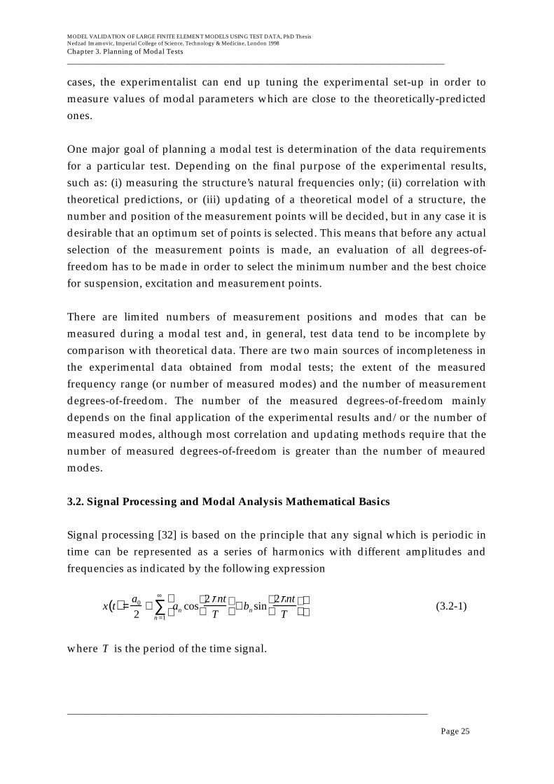
Signal processing [32] is based on the principle that any signal which is periodic intime can be represented as a series of harmonics with different amplitudes andfrequencies as indicated by the following expression
x t( ) =a0
2+ an cos
2πnt
T
+ bn sin
2πnt
T
n =1
∞
∑ (3.2-1)
where T is the period of the time signal.

MODEL VALIDATION OF LARGE FINITE ELEMENT MODELS USING TEST DATA, PhD ThesisNedzad Imamovic, Imperial College of Science, Technology & Medicine, London 1998
Chapter 3. Planning of Modal Tests__________________________________________________________________________________________
______________________________________________________________________________________
Page 26
In fact, expression (3.2-1) provides the transformation between the time andfrequency domains for a periodic time signal, x t( ) , where the coefficients an and bn
can be found as functions of a known x t( ) via the following expressions:
an =2
T
x t( )
0
T
∫ cos2πnt
T
dt (3.2-2a)
bn =2
T
x t( )
0
T
∫ sin2πnt
T
dt (3.2-2b)
In the case that x t( ) is discretised and defined only at a set of N time points,tk, (k = 1, N) , the Discrete Fourier Transformation (DFT) has to be employed which is
defined as
xk = x tk( )( )=a0
2+ an cos
2πntkT
+ bn sin
2πntk
T
n =1
N / 2
∑ k = 1,. .. N (N even) (3.2-3)
The coefficients an and bn are called Fourier or Spectral coefficients for the function,
x t( ) . The measurement signals (accelerometer and force transducer outputs) are in
the time domain and the corresponding spectral properties are in the frequencydomain.
During measurement, the accelerometer and force time signals are digitised andrecorded for a set of N evenly-spaced time values in the period, T . Assuming thatthe measured signal is periodic in time T , there is a simple relationship between thefrequency range 0 − ωmax( ) and the resolution of the analyser with the number of
discrete values N( ) and sample length T( ) , described by the following expressions:
ωmax =1
2
2πN
T
(3.2-4)
∆ω =2πT
(3.2-5)
The above equations show the limitation when measurement of the higherfrequency responses is attempted.

MODEL VALIDATION OF LARGE FINITE ELEMENT MODELS USING TEST DATA, PhD ThesisNedzad Imamovic, Imperial College of Science, Technology & Medicine, London 1998
Chapter 3. Planning of Modal Tests__________________________________________________________________________________________
______________________________________________________________________________________
Page 27
The basic equation for solution of the Fourier or Spectral coefficients is of thefollowing form:
x1
.
.
xN
=
0.5 cos 2π / T( )..... .
.. .
0.5 cos 2Nπ / T( )
a0
a1
b1
.
(3.2-6)
Discrete Fourier Transform analysis can lose on accuracy when applied toexperimental data and this loss of accuracy can magnify during the analysis iftransient signals are not properly treated. These effects are known as (a) aliasing and(b) leakage. The treatment methods for the above features are windowing, zooming,averaging and filtering. For more details about these properties of the DiscreteFourier Transformation can be found in reference [2],[32].
The Frequency Response Function (FRF) is defined as the ratio of the FourierTransforms of the response and the excitation signal, or, mathematically stated:
Hij ω( ) =Xi ω( )Fj ω( )
, Fk ω( ) = 0, k = 1,.. . N, k ≠ j (3.2-7)
Once the measured FRFs are obtained by experiment, they need to be furtheranalysed in order to extract the modal parameters, which consists of the naturalfrequencies, damping factors and mode shapes. There are several methods forextraction of the modal parameters from these response data and selection of amethod for the analysis depends on the influence of damping on the FRFs, thepresence of close modes etc.. It is important to be aware that some modal parameterextraction methods do not consider the influence of the out-of-range modes whileothers compensate for the residual terms and this indicates that the response modelis more general than the equivalent modal model. Having estimated the modalparameters of individual FRFs, derivation of the experimental mode shapes isrelatively simple and animation of the experimental modes can be performed.
MODEL VALIDATION OF LARGE FINITE ELEMENT MODELS USING TEST DATA, PhD ThesisNedzad Imamovic, Imperial College of Science, Technology & Medicine, London 1998
Chapter 3. Planning of Modal Tests__________________________________________________________________________________________
______________________________________________________________________________________
Page 28
3.3. Pre-Test Planning Mathematical Background
3.3.1. Time and Frequency Domains Relationship
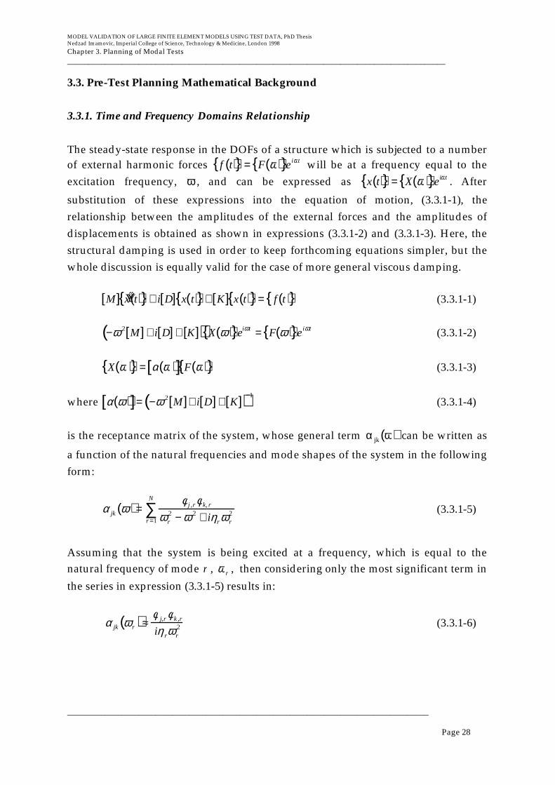
The steady-state response in the DOFs of a structure which is subjected to a numberof external harmonic forces f t( ){ }= F ω( ){ }eiωt will be at a frequency equal to theexcitation frequency, ω , and can be expressed as x t( ){ }= X ω( ){ }eiωt . After
substitution of these expressions into the equation of motion, (3.3.1-1), therelationship between the amplitudes of the external forces and the amplitudes ofdisplacements is obtained as shown in expressions (3.3.1-2) and (3.3.1-3). Here, thestructural damping is used in order to keep forthcoming equations simpler, but thewhole discussion is equally valid for the case of more general viscous damping.
M[ ] Ý Ý x t( ){ }+ i D[ ] x t( ){ }+ K[ ] x t( ){ }= f t( ){ } (3.3.1-1)
−ω 2 M[ ]+ i D[ ]+ K[ ]( ) X ω( ){ }eiωt = F ω( ){ }eiωt (3.3.1-2)
X ω( ){ }= α ω( )[ ] F ω( ){ } (3.3.1-3)
where α ω( )[ ]= −ω 2 M[ ]+ i D[ ]+ K[ ]( )−1 (3.3.1-4)
is the receptance matrix of the system, whose general term α jk ω( ) can be written as
a function of the natural frequencies and mode shapes of the system in the followingform:
α jk ω( )=φ j ,rφk, r
ωr2 − ω 2 + iηrω r
2r =1
N
∑ (3.3.1-5)
Assuming that the system is being excited at a frequency, which is equal to thenatural frequency of mode r , ωr , then considering only the most significant term in
the series in expression (3.3.1-5) results in:
α jk ω r( )≈φ j,r φk ,r
iηrωr2 (3.3.1-6)
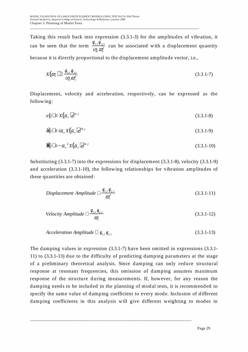
MODEL VALIDATION OF LARGE FINITE ELEMENT MODELS USING TEST DATA, PhD ThesisNedzad Imamovic, Imperial College of Science, Technology & Medicine, London 1998
Chapter 3. Planning of Modal Tests__________________________________________________________________________________________
______________________________________________________________________________________
Page 29
Taking this result back into expression (3.3.1-3) for the amplitudes of vibration, it
can be seen that the term φ i, rφ j, r
iηr ωr2 can be associated with a displacement quantity
because it is directly proportional to the displacement amplitude vector, i.e.,
X ω r( )∝φ i,r φ j,r
iηrω r2 (3.3.1-7)
Displacement, velocity and acceleration, respectively, can be expressed as thefollowing:
x t( ) = X ωr( )eiω r t (3.3.1-8)
Ý x t( ) = iωr X ωr( )eiω rt (3.3.1-9)
Ý Ý x t( ) = −ω r2 X ω r( )eiω rt (3.3.1-10)
Substituting (3.3.1-7) into the expressions for displacement (3.3.1-8), velocity (3.3.1-9)and acceleration (3.3.1-10), the following relationships for vibration amplitudes ofthese quantities are obtained:
Displacement Amplitude ∝φi ,r φ j ,r
ωr2 (3.3.1-11)
Velocity Amplitude ∝φ i,r φ j ,r
ωr
(3.3.1-12)
Acceleration Amplitude ∝ φ i,rφ j ,r (3.3.1-13)
The damping values in expression (3.3.1-7) have been omitted in expressions (3.3.1-11) to (3.3.1-13) due to the difficulty of predicting damping parameters at the stageof a preliminary theoretical analysis. Since damping can only reduce structuralresponse at resonant frequencies, this omission of damping assumes maximumresponse of the structure during measurements. If, however, for any reason thedamping needs to be included in the planning of modal tests, it is recommended tospecify the same value of damping coefficient to every mode. Inclusion of differentdamping coefficients in this analysis will give different weighting to modes in
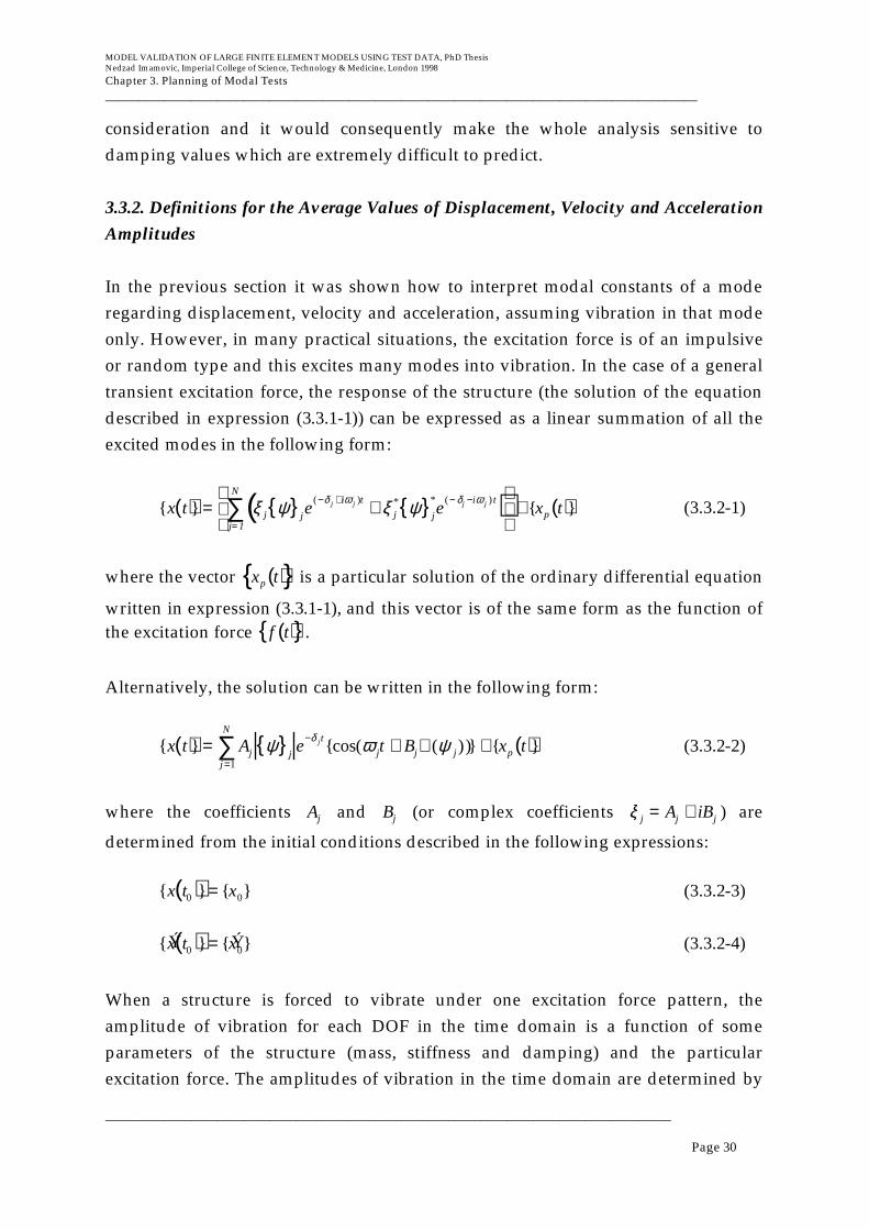
MODEL VALIDATION OF LARGE FINITE ELEMENT MODELS USING TEST DATA, PhD ThesisNedzad Imamovic, Imperial College of Science, Technology & Medicine, London 1998
Chapter 3. Planning of Modal Tests__________________________________________________________________________________________
______________________________________________________________________________________
Page 30
consideration and it would consequently make the whole analysis sensitive todamping values which are extremely difficult to predict.
3.3.2. Definitions for the Average Values of Displacement, Velocity and Acceleration
Amplitudes
In the previous section it was shown how to interpret modal constants of a moderegarding displacement, velocity and acceleration, assuming vibration in that modeonly. However, in many practical situations, the excitation force is of an impulsiveor random type and this excites many modes into vibration. In the case of a generaltransient excitation force, the response of the structure (the solution of the equationdescribed in expression (3.3.1-1)) can be expressed as a linear summation of all theexcited modes in the following form:
{x t( )} = ξ j ψ{ }je(−δ j +iω j )t + ξ j
* ψ{ }j
*e
(− δj −iω j ) t( )j= 1
N
∑
+ {xp t( )} (3.3.2-1)
where the vector xp t( ){ } is a particular solution of the ordinary differential equation
written in expression (3.3.1-1), and this vector is of the same form as the function ofthe excitation force f t( ){ }.
Alternatively, the solution can be written in the following form:
{x t( )} = Aj ψ{ }je
−δ j t{cos(ω jt + Bj∠(ψ j))j =1
N
∑ } + {xp t( )} (3.3.2-2)
where the coefficients Aj and Bj (or complex coefficients ξ j = Aj + iBj ) are
determined from the initial conditions described in the following expressions:
{x t0( )}= {x0} (3.3.2-3)
{Ý x t0( )} = { Ý x 0} (3.3.2-4)
When a structure is forced to vibrate under one excitation force pattern, theamplitude of vibration for each DOF in the time domain is a function of someparameters of the structure (mass, stiffness and damping) and the particularexcitation force. The amplitudes of vibration in the time domain are determined by

MODEL VALIDATION OF LARGE FINITE ELEMENT MODELS USING TEST DATA, PhD ThesisNedzad Imamovic, Imperial College of Science, Technology & Medicine, London 1998
Chapter 3. Planning of Modal Tests__________________________________________________________________________________________
______________________________________________________________________________________
Page 31
the natural frequencies and mode shapes which are simple functions of thestructural and geometrical properties (mass, stiffness and damping) of the structureunder investigation. This shows that for a particular excitation there will be onepattern of amplitudes of vibration in the time domain which is determined by thecontributions of all the modes in the frequency domain. Therefore, in order topredict the average response at a DOF for displacement of the structure for a generalexcitation which would excite modes over a wide frequency range, the AverageDriving DOF Displacement (ADDOFD) level can be defined as the average sum ofall contributing modes as shown in the following expression:
ADDOFD( j) =φ jr
2
ω r2
r=1
m
∑ (3.3.2-5)
Similarly, the Average Driving DOF Velocity (ADDOFV) parameter is defined by:
ADDOFV( j) =φ jr
2
ωrr=1
m
∑ (3.3.2-6)
and it should be noted that the ADDOFV coefficient is the same as the AverageDriving Point Residue (ADPR) coefficient, described in detail in reference [33].
Finally, the Average Driving DOF Acceleration coefficient (ADDOFA) describes theaverage acceleration of the response and the parameter can be defined by thefollowing expression:
ADDOFA( j) = φ jr2
r =1
m
∑ (3.3.2-7)
The reason for assigning the label ’average’ to all the three above-defined parametersis because there are several modes which contribute to the whole response signal.Usually, when the structure is excited by an impulsive force, not all modescontribute to the response because some of the modes from the excitation frequencyrange are not excited for some reason (such as a poor choice of the excitationposition).
The ADDOFD, ADDOFV and ADDOFA parameters define the ’average’ amplitudesof the imaginary response caused by an hypotetically impulsive excitation which
MODEL VALIDATION OF LARGE FINITE ELEMENT MODELS USING TEST DATA, PhD ThesisNedzad Imamovic, Imperial College of Science, Technology & Medicine, London 1998
Chapter 3. Planning of Modal Tests__________________________________________________________________________________________
______________________________________________________________________________________
Page 32
would act on all DOFs simultaneously and therefore would excite all modes fromthe excitation frequency range.
3.4. Optimum Suspension Positions
Determination of the optimum suspension positions is a process of finding anarrangement such that particular boundary conditions can be achieved duringtesting. In many practical situations, the boundary conditions sought during testingare free-free and these are best approximated by suspending the structure on softsprings. The major difficulty is to find positions on the structure where thesesuspension springs should be attached, since any connection to the structure caninterfere with its response and produce different dynamic parameters to thosewhich should apply for the true free-free boundary conditions.
3.4.1. Testing for Free-Free Boundary Conditions
The free-free boundary conditions are the most common type of boundaryconditions in practice. Theoretically, under these boundary conditions the structureis not connected to any other object and it is clear that this cannot be achieved inpractice, apart from few situations where some form of non-contact force field isestablished to position test piece (e.g. magnetic field). Another situation wheretheoretically free-free boundary conditions could be achieved is testing in the zerogravity space. These special situations of achievable free-free boundary conditionswithout connection of the test piece to other objects are extremely rare and limitedthat their significance has a pure academic character.
In order to simulate free-free boundary conditions using some form of connection ofthe test piece to other objects, it would be necessary that each attachment location issituated on or very close to the nodal lines of all excited modes during testing. Thenodal line of a mode is defined as a set of all DOFs inside geometrical domain of thestructure which have zero amplitudes of vibration. When the structure is excited,several modes contribute to the time response, but since these modes contribute atdifferent frequencies and they may have arbitrary phase difference between them(which is determined by the initial conditions, (3.3.2-3) and (3.3.2-4)), there is noguarantee that it is possible to find locations on the structure which have a totalresponse equal to zero. If such locations existed then they would be the optimumsuspension locations to achieve free-free boundary conditions. Hence, locations

MODEL VALIDATION OF LARGE FINITE ELEMENT MODELS USING TEST DATA, PhD ThesisNedzad Imamovic, Imperial College of Science, Technology & Medicine, London 1998
Chapter 3. Planning of Modal Tests__________________________________________________________________________________________
______________________________________________________________________________________
Page 33
which have minimum total response seem to be the optimum choice foraccomplishment of free-free boundary conditions. Since the ‘average’ amplitude oftotal response (in terms of displacements) is defined by ADDOFD, this parametercan be used to find optimum suspension locations.
The optimum suspension locations for modal testing are generally to be found in theregions of a structure where the average displacement is the lowest, i.e. in thoseregions which are defined by low values of the ADDOFD coefficient. Unfortunately,as far as a suspension locations are concerned, there are physical limitations thatrestrict how and where the structure can be suspended and, usually, the number ofpossibilities for practical suspension attachments is small.
Optimum suspension = minj
ADDOFD( j)( ) (3.4.1-1)
The use of the ADDOFD function to find optimum locations is conservative since itassumes the worst case scenario, which is that all modes contribute to the totalresponse. The probability of this happening in practice is low and any degrees-of-freedom which have a low value of the ADDOFD coefficient when all modes arecontributing can have only even lower values if some modes are not excited, as isthe case in many practical situations.
3.5. Optimum Driving Positions
3.5.1. General Requirements for Optimum Excitation Positions
There are two main types of excitation for structures in respect to the input ofexcitation energy: (i) the non-destructive impact from an external source and (ii) thenon-destructive attachment to an external source. Apart from these excitations withphysical connections to the structure, there are some other excitation techniqueswhich do not require physical contact between the test structure and the source ofexcitation and these include: (i) excitations by magnetic field and (ii) excitations bysound waves or air pressure.
The process of energy transfer from an excitation source to a structure's modes is arather complicated process but there are a few major features which characterise it.Whether an excitation is impact- or continuous force-like, the excitation must notcause any permanent damage to the tested structure, not even in the vicinity of the

MODEL VALIDATION OF LARGE FINITE ELEMENT MODELS USING TEST DATA, PhD ThesisNedzad Imamovic, Imperial College of Science, Technology & Medicine, London 1998
Chapter 3. Planning of Modal Tests__________________________________________________________________________________________
______________________________________________________________________________________
Page 34
impact locations. The most common damage which occurs during a modal test iswhen a hammer excitation is used to excite high-frequency modes. In order to avoiddouble-hit effects and to have short enough impact times to excite the high-frequency modes, it is necessary to use a hard metal tip on the hammer. Thestructure should be checked during the test to make sure there are no permanentdeformations caused by the metal tip of the hammer. Another example of possibledamage during modal testing is the use of a shaker on lightly damped structuresnear resonant frequencies. This can cause such large deformations at frequenciesclose to and at resonances that these can consequently cause permanent damage tostructures.
Process of Energy Transfer during Excitation
The exact process of energy transfer from the excitation source to each mode of thestructure involves complex energy transformations during the vibration process.When a structure is excited by an impact, for instance, a certain amount of energy istransferred from the excitation source to the structure. If we assume that there is noloss of energy in plastic deformations at the excitation position, or in sound and heatduring the impact process, then all energy input to the structure will be transferredinto strain and/or kinetic energy at the vicinity of the excitation position. Thiskinetic and strain energy will initiate vibrations of the adjacent degrees-of-freedomand that will consequently cause generation of mechanical waves and theirdistribution throughout the domain of the whole structure. These waves will reflectat the boundaries of the structure and will interact among themselves until somekind of steady-state wave transmission pattern is established. In the frequencydomain the general response of the structure can be separated into several frequencyresponses or modes. Since the speed of both the longitudinal and transverse wavesin most practical materials is quite high, this will make the transmission time of theboth waves a short period of time, it can be assumed that the distribution of energythroughout the domain of a structure and the establishment of all modes is almostinstantaneous.
There are many factors which determine the distribution of energy into the modes,such as: (i) the level of damping of the structure, (ii) the elastic properties of thestructure, (iii) the mass distribution, (iv) the homogeneouisity of the density andelastic properties throughout the domain, (v) the isotropy of the structural

MODEL VALIDATION OF LARGE FINITE ELEMENT MODELS USING TEST DATA, PhD ThesisNedzad Imamovic, Imperial College of Science, Technology & Medicine, London 1998
Chapter 3. Planning of Modal Tests__________________________________________________________________________________________
______________________________________________________________________________________
Page 35
properties, (vi) any known or unknown imperfections such as cracks, pre-stresslevels and deformations and (vii) other factors like current temperature, etc..
In reality, it is impossible to predict effects of all these factors accurately in order tooptimise the excitation position for a modal test, but it is known that one of thefactors which determines the amount of energy received by each mode is the relativeposition of an excitation source to each mode shape. It is known that if a source ofexcitation is close to or at a nodal line of a mode, then little or no energy will betransferred to that mode which, consequently, will not be registered in the measuredresponse. Other commonly-observed effects of the excitation position upon thewhole vibration process during a modal test are so-called ’double-hit’ by a hammeror interference caused by interaction between the shaker and the structure.Several new techniques to select an optimum driving position for the excitation of asmany modes as possible within a specified frequency range are presented in thefollowing sections.
3.5.2. Hammer Excitation
Apart from a general requirement to avoid excitation positions near any nodal lineson the structure, there is a common experience that regions of high average velocityshould be avoided since hitting in the vicinity of these positions can cause the so-called ‘double-hit’ effect. Therefore, the ADDOFV parameter can be of help whendeciding where not to excite a structure using a hammer, and regions of high valuesof this parameter should be avoided.
3.5.3. Shaker Excitation
The general requirement for avoiding excitation close to any nodal lines applies alsofor excitation using a shaker, but it is also necessary to minimise the interference of ashaker with a structure during vibration testing. Since a shaker is, in fact, essentiallya simple mass-spring-damper attached to the test structure, the least interference ofthe shaker will have or would occur if the shaker is attached to a region where theaverage acceleration, the ADDOFA parameter, has a minimum value. Therefore, theADDOFA parameter can be used when deciding where not to attach a shaker to astructure.

MODEL VALIDATION OF LARGE FINITE ELEMENT MODELS USING TEST DATA, PhD ThesisNedzad Imamovic, Imperial College of Science, Technology & Medicine, London 1998
Chapter 3. Planning of Modal Tests__________________________________________________________________________________________
______________________________________________________________________________________
Page 36
3.5.4. Optimum Driving Point (ODP) Technique
The Optimum Driving Point (ODP) technique is designed to identify positionswhich are close to or on the nodal lines of any mode within a specified frequencyrange. Hence, the values of the modal constants for degrees-of-freedom which areclose to or on nodal lines of a mode will be close to zero. In order to describe theposition of any DOF in respect to the position of nodal lines of all modes, modalconstants for all selected modes at each DOF are multiplied together and theresulting value is a coefficient called the ODP parameter for each DOF.Mathematically, the ODP method is based on the following expression:
ODP i( )= φ i,rr =1
m
∏ (3.5.4-1)
The DOFs which have ODP value close to zero are the DOFs which are close to or ona nodal line and, consequently, should be avoided as possible excitation positions.Contrary to the above-mentioned DOFs, the positions which have values of the ODPparameter which are different to zero are those which should be considered aspossible excitation positions since they are not close to the nodal lines of any modein the specified frequency range.
3.5.5. Non-Optimum Driving Point (NODP) Technique
The NODP technique is based on a similar principle for assessment of the optimumdriving point to that used for the ODP technique: the method defines a parameterfor each DOF which describes how close that DOF is to a nodal line of any modewithin a specified frequency range. This method selects the minimum absolute valueof the modal constants for all selected modes for a DOF and defines that value as theNODP parameter for that DOF. Mathematically, the method is based on thefollowing expression:
NODP i( ) = minr
φ i, r( ) (3.5.5-1)
It can be seen from the above expression that this parameter does not average all themodal constants but shows only the lowest-valued from all modes underconsideration. The values of this parameter do not show how good a particularposition is as a driving point, but they show how poor each DOF is in that role.
MODEL VALIDATION OF LARGE FINITE ELEMENT MODELS USING TEST DATA, PhD ThesisNedzad Imamovic, Imperial College of Science, Technology & Medicine, London 1998
Chapter 3. Planning of Modal Tests__________________________________________________________________________________________
______________________________________________________________________________________
Page 37
Therefore, if a DOF has a low value of the NODP parameter, this means that thisDOF is not suitable as a possible driving position. In contrast, if a DOF has a highvalue of NODP, this does not necessarily mean that this DOF is automatically thebest driving position. This is the reason for naming this method the Non-OptimumDriving Point (NODP), because it shows which points are not optimum rather thanassessing an average value for all modes under consideration.
3.5.6. Determination of the Optimum Driving Positions
The ODP and NODP parameters essentially consider only positions of the nodallines of all modes under consideration in order to discriminate DOFs as potentiallygood or bad excitation positions. These techniques do not consider the actual energytransfer from the excitation source to a test piece in order to select the optimumexcitation location. Although it is very important that the excitation position is notset close to or on any of the nodal lines, there are some additional effects which haveto be taken into account when selecting this position. If a hammer excitation is to beused, then there is a possibility of a double-hit if the excitation is applied inside ahigh-velocity region of a structure. If, however, a shaker is used for excitation, thenthere is a requirement for the interference of the shaker with the structure beingtested to be minimised. Since a shaker can be considered as a simple mass-spring-damper attached to the test structure, it is clear that the least interference would becaused if the shaker is attached to the structure in the region where the averageacceleration is lowest.
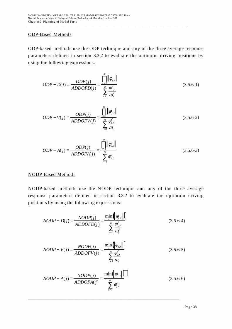
MODEL VALIDATION OF LARGE FINITE ELEMENT MODELS USING TEST DATA, PhD ThesisNedzad Imamovic, Imperial College of Science, Technology & Medicine, London 1998
Chapter 3. Planning of Modal Tests__________________________________________________________________________________________
______________________________________________________________________________________
Page 38
ODP-Based Methods
ODP-based methods use the ODP technique and any of the three average responseparameters defined in section 3.3.2 to evaluate the optimum driving positions byusing the following expressions:
ODP − D( j) =ODP( j)
ADDOFD( j)=
φ j ,rr =1
m
∏φ j ,r
2
ω r2
r =1
m
∑(3.5.6-1)
ODP − V( j) =ODP( j)
ADDOFV( j)=
φ j ,rr= 1
m
∏φ j ,r
2
ω rr =1
m
∑(3.5.6-2)
ODP − A( j) =ODP( j)
ADDOFA( j)=
φ j, rr= 1
m
∏φ j, r
2
r= 1
m
∑(3.5.6-3)
NODP-Based Methods
NODP-based methods use the NODP technique and any of the three averageresponse parameters defined in section 3.3.2 to evaluate the optimum drivingpositions by using the following expressions:
NODP − D( j) =NODP( j)
ADDOFD( j )=
minr
φ j ,r( )φ j, r
2
ω r2
r= 1
m
∑(3.5.6-4)
NODP − V( j) =NODP( j)
ADDOFV( j )=
minr
φ j ,r( )φ j, r
2
ω rr= 1
m
∑(3.5.6-5)
NODP − A( j) =NODP( j)
ADDOFA( j)=
minr
φ j ,r( )φ j ,r
2
r =1
m
∑(3.5.6-6)

MODEL VALIDATION OF LARGE FINITE ELEMENT MODELS USING TEST DATA, PhD ThesisNedzad Imamovic, Imperial College of Science, Technology & Medicine, London 1998
Chapter 3. Planning of Modal Tests__________________________________________________________________________________________
______________________________________________________________________________________
Page 39
3.5.7. Application of the ODP and NODP Techniques
Both the ODP and NODP techniques have been applied to several test casestructures in order to identify the optimum driving point(s) for modal testing. Asimple plate structure was used to demonstrate the application of the proposedmethods for the optimisation of modal testing. It should be noted that in majoritycases presented here regions indicated in RED are not the optimum as defined bythe methods used.
Simple Plate
The geometry of the simple plate used as a test case can be seen in Figure 3.5.7-1. Weshall assume that a modal test is to be performed on the structure and that all modesin the range 0-200 Hz should be measured. Preliminary analysis predicts severalmodes in that range, and these are given in Figure 3.5.7-1. Since the prediction of thepreliminary mode shapes could be incomplete, i.e. not all modes from the frequencyrange might be predicted, another two modes with higher natural frequencies wereincluded in the analysis to allow for the possibility of inaccurate predictions. Allmode shapes used in the analysis are out-of-plane modes.
The Average Displacement, Velocity and Acceleration Estimates
Estimates of the average displacement, velocity and acceleration quantities areindicated by the values of the ADDOFD, ADDOFV and ADDOFA parameters, andare given in Figures 3.5.7-2, -3 and -4, respectively. All three contour diagramsindicate that the edges of the plate, and particularly the corners have higher averageresponse levels than elsewhere, while the inner area of the plate has low averageresponse level. There is a significant difference between the contours for the averagedisplacement, velocity and acceleration parameters in the size of the central regionof low response values. It can be seen from the pictures that the average accelerationcontours have the largest area of low signal values, while the average displacementcontour has the smallest area. It should be noted here that the optimum suspensionposition of the structure is considered to be in the area of the lowest averagedisplacement values, which is clearly defined in Figure 3.5.7-2. The average velocitycontours can help to identify the regions where the possibility of the double-hit by ahammer

MODEL VALIDATION OF LARGE FINITE ELEMENT MODELS USING TEST DATA, PhD ThesisNedzad Imamovic, Imperial College of Science, Technology & Medicine, London 1998
Chapter 3. Planning of Modal Tests__________________________________________________________________________________________
______________________________________________________________________________________
Page 40
Figure 3.5.7-1. Mode Shape Nodal Lines of Simple Plate.

MODEL VALIDATION OF LARGE FINITE ELEMENT MODELS USING TEST DATA, PhD ThesisNedzad Imamovic, Imperial College of Science, Technology & Medicine, London 1998
Chapter 3. Planning of Modal Tests__________________________________________________________________________________________
______________________________________________________________________________________
Page 41
excitation is high and should be avoided. The average acceleration contours canhelp to find the best place to attach a shaker to excite the structure as well as suitableplaces for transducer locations where the average response signal strength is high, inorder to minimise the noise-to-signal ratio and to improve the accuracy of the test.
Figure 3.5.7-2. ADDOFD of Simple Plate.
Figure 3.5.7-3. ADDOFV of Simple Plate.
Figure 3.5.7-4. ADDOFA of Simple Plate.
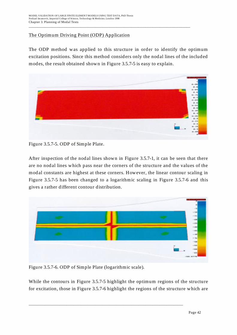
MODEL VALIDATION OF LARGE FINITE ELEMENT MODELS USING TEST DATA, PhD ThesisNedzad Imamovic, Imperial College of Science, Technology & Medicine, London 1998
Chapter 3. Planning of Modal Tests__________________________________________________________________________________________
______________________________________________________________________________________
Page 42
The Optimum Driving Point (ODP) Application
The ODP method was applied to this structure in order to identify the optimumexcitation positions. Since this method considers only the nodal lines of the includedmodes, the result obtained shown in Figure 3.5.7-5 is easy to explain.
Figure 3.5.7-5. ODP of Simple Plate.
After inspection of the nodal lines shown in Figure 3.5.7-1, it can be seen that thereare no nodal lines which pass near the corners of the structure and the values of themodal constants are highest at these corners. However, the linear contour scaling inFigure 3.5.7-5 has been changed to a logarithmic scaling in Figure 3.5.7-6 and thisgives a rather different contour distribution.
Figure 3.5.7-6. ODP of Simple Plate (logarithmic scale).
While the contours in Figure 3.5.7-5 highlight the optimum regions of the structurefor excitation, those in Figure 3.5.7-6 highlight the regions of the structure which are
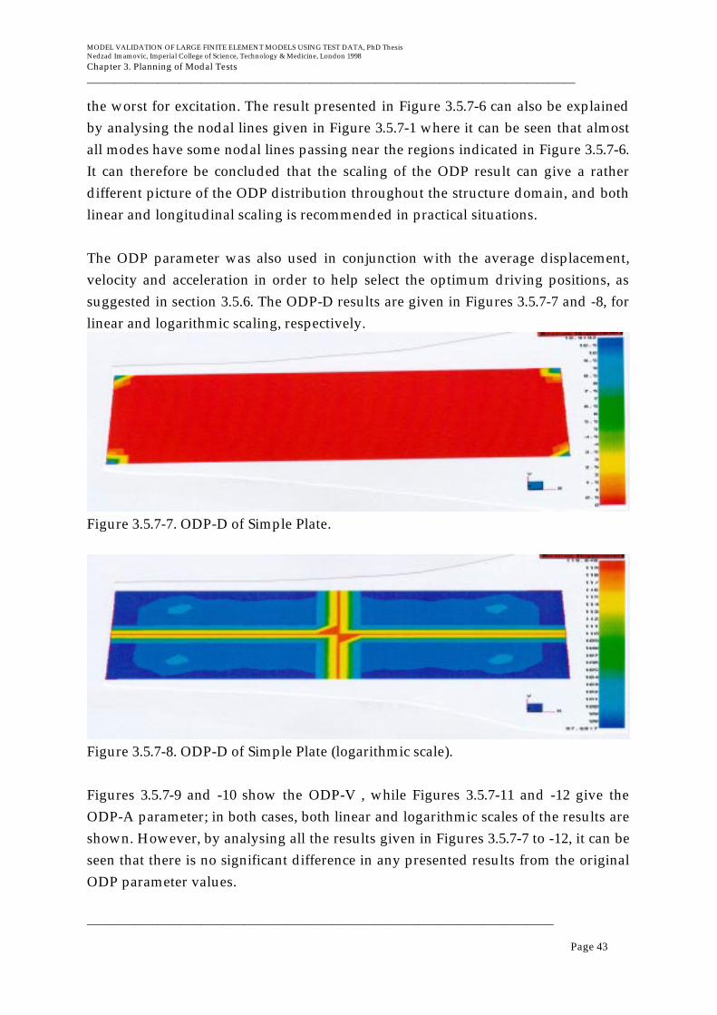
MODEL VALIDATION OF LARGE FINITE ELEMENT MODELS USING TEST DATA, PhD ThesisNedzad Imamovic, Imperial College of Science, Technology & Medicine, London 1998
Chapter 3. Planning of Modal Tests__________________________________________________________________________________________
______________________________________________________________________________________
Page 43
the worst for excitation. The result presented in Figure 3.5.7-6 can also be explainedby analysing the nodal lines given in Figure 3.5.7-1 where it can be seen that almostall modes have some nodal lines passing near the regions indicated in Figure 3.5.7-6.It can therefore be concluded that the scaling of the ODP result can give a ratherdifferent picture of the ODP distribution throughout the structure domain, and bothlinear and longitudinal scaling is recommended in practical situations.
The ODP parameter was also used in conjunction with the average displacement,velocity and acceleration in order to help select the optimum driving positions, assuggested in section 3.5.6. The ODP-D results are given in Figures 3.5.7-7 and -8, forlinear and logarithmic scaling, respectively.
Figure 3.5.7-7. ODP-D of Simple Plate.
Figure 3.5.7-8. ODP-D of Simple Plate (logarithmic scale).
Figures 3.5.7-9 and -10 show the ODP-V , while Figures 3.5.7-11 and -12 give theODP-A parameter; in both cases, both linear and logarithmic scales of the results areshown. However, by analysing all the results given in Figures 3.5.7-7 to -12, it can beseen that there is no significant difference in any presented results from the originalODP parameter values.

MODEL VALIDATION OF LARGE FINITE ELEMENT MODELS USING TEST DATA, PhD ThesisNedzad Imamovic, Imperial College of Science, Technology & Medicine, London 1998
Chapter 3. Planning of Modal Tests__________________________________________________________________________________________
______________________________________________________________________________________
Page 44
Figure 3.5.7-9. ODP-V of Simple Plate.
Figure 3.5.7-10. ODP-V of Simple Plate (logarithmic scale).
Figure 3.5.7-11. ODP-A of Simple Plate.
Figure 3.5.7-12. ODP-A of Simple Plate (logarithmic scale).

MODEL VALIDATION OF LARGE FINITE ELEMENT MODELS USING TEST DATA, PhD ThesisNedzad Imamovic, Imperial College of Science, Technology & Medicine, London 1998
Chapter 3. Planning of Modal Tests__________________________________________________________________________________________
______________________________________________________________________________________
Page 45
The Non-Optimum Driving Point (NODP) Application
The NODP method was applied to this test case and the results are given in Figures3.5.7-13 and -14 for linear and logarithmic scales, respectively.
Figure 3.5.7-13. NODP of Simple Plate.
Figure 3.5.7-14. NODP of Simple Plate (logarithmic scale).
The linear scale contours of the NODP parameter values indicate several regions ofthe structure where the NODP parameter values are different to zero. The regions ofthe structure where the NODP values are close to zero are the regions which aredefinitely not suitable for excitation. This parameter indicates the regions of thestructure which should not be selected as excitation positions but the rest of thestructure, in which the values of the NODP parameter are greater than zero, shouldnot be taken as necessarily being good excitation positions. As expected, the logscale of the NODP parameter results indicates that the two central lines are of verylow value compared with the rest of the structure.

MODEL VALIDATION OF LARGE FINITE ELEMENT MODELS USING TEST DATA, PhD ThesisNedzad Imamovic, Imperial College of Science, Technology & Medicine, London 1998
Chapter 3. Planning of Modal Tests__________________________________________________________________________________________
______________________________________________________________________________________
Page 46
Application of the NODP method in conjunction with the average displacement,velocity and acceleration parameters was carried out in order to determine theoptimum excitation positions using these criteria. Division of the NODP parameterby the ADDOFD parameter gives new contours, as shown in Figures 3.5.7-15 and -16for linear and log scales, respectively.
Figure 3.5.7-15. NODP-D of Simple Plate.
Figure 3.5.7-16. NODP-D of Simple Plate (logarithmic scale).
Analysing the nodal lines of all modes given in Figure 3.5.7-1, it can be concludedthat there are no nodal lines near the indicated excitation locations; furthermore,considering the distribution of the average displacement value, it can be concludedthat the ADDOFD values are low at these locations. The log scale of NODP-D plotsindicate again the regions of the structure where the concentration of nodal lines ishigh for the included modes, and the excitation position should not be placed closeto these central regions of the structure, as shown in Figure 3.5.7-16.
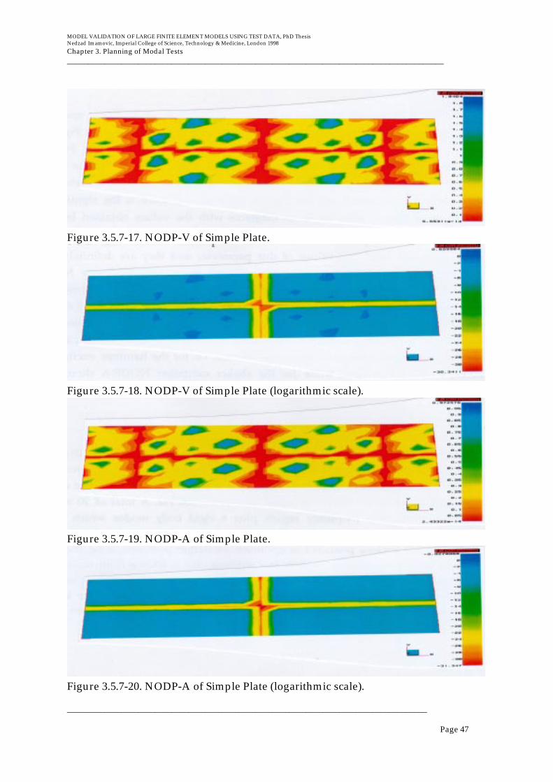
MODEL VALIDATION OF LARGE FINITE ELEMENT MODELS USING TEST DATA, PhD ThesisNedzad Imamovic, Imperial College of Science, Technology & Medicine, London 1998
Chapter 3. Planning of Modal Tests__________________________________________________________________________________________
______________________________________________________________________________________
Page 47
Figure 3.5.7-17. NODP-V of Simple Plate.
Figure 3.5.7-18. NODP-V of Simple Plate (logarithmic scale).
Figure 3.5.7-19. NODP-A of Simple Plate.
Figure 3.5.7-20. NODP-A of Simple Plate (logarithmic scale).

MODEL VALIDATION OF LARGE FINITE ELEMENT MODELS USING TEST DATA, PhD ThesisNedzad Imamovic, Imperial College of Science, Technology & Medicine, London 1998
Chapter 3. Planning of Modal Tests__________________________________________________________________________________________
______________________________________________________________________________________
Page 48
The NODP-V parameter is shown in Figures 3.5.7-17 and -18 for linear and logscaling respectively, produced almost identical results to those shown in Figures3.5.7-15 and -16 for NODP-D. Also, the NODP-A parameter as shown in Figure3.5.7-19 and 3.5.7-20 indicates very similar results to those given in Figures 3.5.7-15to -18. Although the contours obtained by dividing the NODP parameter by threedifferent parameters are similar but not identical, there is the significant differenceof how to compare these diagrams with the values obtained by the ODP method. Asexplained earlier, the NODP values indicate regions of the structure which have lowvalues of this parameter and they are definitely not suitable as potential excitationpositions. Since neither the ODP nor NODP method consider the energy transferfrom the excitation source to the structure, it is necessary to check several locationsindicated by the NODP method as potentially good excitation positions, i.e. thelocations which have non-zero values of the NODP parameter. Depending upon thetype of the excitation method, the relevant diagram should be selected, i.e. for thehammer excitation, NODP-V should be used, while for the shaker excitation NODP-A should be selected for determination of the optimum driving location.
Engine Casing
Application of the ODP and NODP methods in order to choose the optimumexcitation locations for a modal test produced results which were confirmed by atest carried out earlier. The natural frequencies and mode shapes of engine casingwere calculated in the frequency region within 0 - 180 Hz. A total of 20 modes werefound in this frequency region plus 6 rigid body modes which were excluded fromthe analysis. The ODP results are given in Figure 3.5.7-21 in a log scale. The tworegions predicted as optimum excitation positions using the ODP method are theregions of extremely low stiffness (this is known from modelling of engine casing)and as such are not very suitable as excitation positions because impact within lowstiffness region can result in mechanical damage to the component. This highlights aweakness of the ODP technique when it is individually used for selection ofoptimum excitation location.
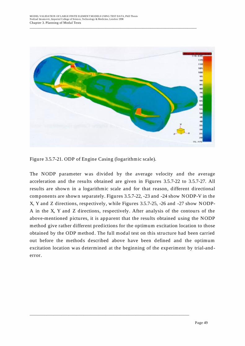
MODEL VALIDATION OF LARGE FINITE ELEMENT MODELS USING TEST DATA, PhD ThesisNedzad Imamovic, Imperial College of Science, Technology & Medicine, London 1998
Chapter 3. Planning of Modal Tests__________________________________________________________________________________________
______________________________________________________________________________________
Page 49
Figure 3.5.7-21. ODP of Engine Casing (logarithmic scale).
The NODP parameter was divided by the average velocity and the averageacceleration and the results obtained are given in Figures 3.5.7-22 to 3.5.7-27. Allresults are shown in a logarithmic scale and for that reason, different directionalcomponents are shown separately. Figures 3.5.7-22, -23 and -24 show NODP-V in theX, Y and Z directions, respectively, while Figures 3.5.7-25, -26 and -27 show NODP-A in the X, Y and Z directions, respectively. After analysis of the contours of theabove-mentioned pictures, it is apparent that the results obtained using the NODPmethod give rather different predictions for the optimum excitation location to thoseobtained by the ODP method. The full modal test on this structure had been carriedout before the methods described above have been defined and the optimumexcitation location was determined at the beginning of the experiment by trial-and-error.

MODEL VALIDATION OF LARGE FINITE ELEMENT MODELS USING TEST DATA, PhD ThesisNedzad Imamovic, Imperial College of Science, Technology & Medicine, London 1998
Chapter 3. Planning of Modal Tests__________________________________________________________________________________________
______________________________________________________________________________________
Page 50
Figure 3.5.7-22. NODP-A (X component) of Engine Casing (logarithmic scale).
Figure 3.5.7-23. NODP-A (Y component) of Engine Casing (logarithmic scale).
Figure 3.5.7-24. NODP-A (Z component) of Engine Casing (logarithmic scale).
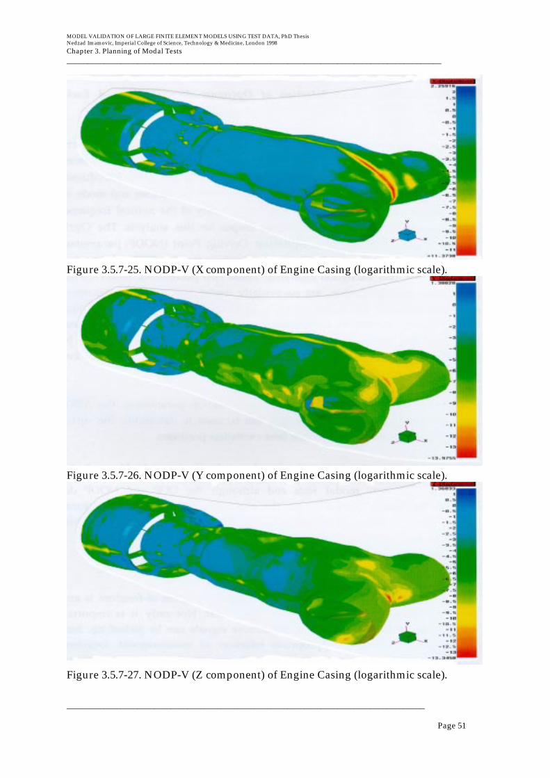
MODEL VALIDATION OF LARGE FINITE ELEMENT MODELS USING TEST DATA, PhD ThesisNedzad Imamovic, Imperial College of Science, Technology & Medicine, London 1998
Chapter 3. Planning of Modal Tests__________________________________________________________________________________________
______________________________________________________________________________________
Page 51
Figure 3.5.7-25. NODP-V (X component) of Engine Casing (logarithmic scale).
Figure 3.5.7-26. NODP-V (Y component) of Engine Casing (logarithmic scale).
Figure 3.5.7-27. NODP-V (Z component) of Engine Casing (logarithmic scale).
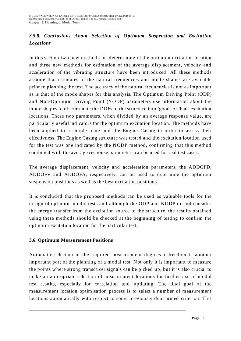
MODEL VALIDATION OF LARGE FINITE ELEMENT MODELS USING TEST DATA, PhD ThesisNedzad Imamovic, Imperial College of Science, Technology & Medicine, London 1998
Chapter 3. Planning of Modal Tests__________________________________________________________________________________________
______________________________________________________________________________________
Page 52
3.5.8. Conclusions About Selection of Optimum Suspension and Excitation
Locations
In this section two new methods for determining of the optimum excitation locationand three new methods for estimation of the average displacement, velocity andacceleration of the vibrating structure have been introduced. All these methodsassume that estimates of the natural frequencies and mode shapes are availableprior to planning the test. The accuracy of the natural frequencies is not as importantas is that of the mode shapes for this analysis. The Optimum Driving Point (ODP)and Non-Optimum Driving Point (NODP) parameters use information about themode shapes to discriminate the DOFs of the structure into ‘good’ or ‘bad’ excitationlocations. These two parameters, when divided by an average response value, areparticularly useful indicators for the optimum excitation location. The methods havebeen applied to a simple plate and the Engine Casing in order to assess theireffectivness. The Engine Casing structure was tested and the excitation location usedfor the test was one indicated by the NODP method, confirming that this methodcombined with the average response parameters can be used for real test cases.
The average displacement, velocity and acceleration parameters, the ADDOFD,ADDOFV and ADDOFA, respectively, can be used to determine the optimumsuspension positions as well as the best excitation positions.
It is concluded that the proposed methods can be used as valuable tools for thedesign of optimum modal tests and although the ODP and NODP do not considerthe energy transfer from the excitation source to the structure, the results obtainedusing these methods should be checked at the beginning of testing to confirm theoptimum excitation location for the particular test.
3.6. Optimum Measurement Positions
Automatic selection of the required measurement degrees-of-freedom is anotherimportant part of the planning of a modal test. Not only it is important to measurethe points where strong transducer signals can be picked up, but it is also crucial tomake an appropriate selection of measurement locations for further use of modaltest results, especially for correlation and updating. The final goal of themeasurement location optimisation process is to select a number of measurementlocations automatically with respect to some previously-determined criterion. This

MODEL VALIDATION OF LARGE FINITE ELEMENT MODELS USING TEST DATA, PhD ThesisNedzad Imamovic, Imperial College of Science, Technology & Medicine, London 1998
Chapter 3. Planning of Modal Tests__________________________________________________________________________________________
______________________________________________________________________________________
Page 53
might be defined as a linearly-independent truncated set of measured mode shapes,and/or the value of signal-to-noise ratio for measurement positions.
3.6.1. Definitions for optimum measurement positions
Before any evaluation of optimum transducer locations can be attempted, it isnecessary to have some preliminary theoretical representation of the dynamicbehaviour of the structure. These preliminary results usually come from a FiniteElement Model (they are called "preliminary" because this might not be the finaltheoretical model of the structure) and this model will be referred to as thepreliminary theoretical model. The full set of all the co-ordinates in this preliminarytheoretical model will be referred to as potential measurement points. These are allthe DOFs at the grid points in the preliminary theoretical model of the structure.
It is clear that some points cannot be measured simply because there is no access tothem, at least with existing experimental techniques, and so there will be a subset ofall the potential measurement points which consists of those DOFs which are
accessible for measurement and these are called possible measurement points.Generally, this set only includes points on the surface of the model and only thosewhich are actually accessible. It will be assumed that all the potential measurementpositions that are inaccessible will be excluded from the selection of the optimummeasurement positions.
3.6.2. Use of Average Displacement, Velocity and Acceleration
It is desirable to minimise the noise-to-signal ratio during the measurements inorder to obtain a reliable set of experimental data. Once again, it is very clear thatmeasurements close to or on nodal lines should be avoided since the strength of theresponse in these regions is low.
In the planning of modal tests it is also important to specify the right measurementquantity (acceleration, velocity or displacement) during the test. In most practicalsituations, acceleration is measured. Transducers (or accelerometers) are placed tomeasure the acceleration response which can be transformed analytically into eitherdisplacement, velocity or acceleration signals, but what is physically measured is theacceleration at the measurement locations. Therefore, the ADDOFA parametershould be used to identify the regions of the structure which have high response

MODEL VALIDATION OF LARGE FINITE ELEMENT MODELS USING TEST DATA, PhD ThesisNedzad Imamovic, Imperial College of Science, Technology & Medicine, London 1998
Chapter 3. Planning of Modal Tests__________________________________________________________________________________________
______________________________________________________________________________________
Page 54
levels and these regions should be considered as potentially good measurementlocations.
In some situations, the actual measurement quantity is velocity, i.e. in the case ofmeasurement being performed using a laser velocimeter. In this case, the sametheory applies as for acceleration transducers, but the average velocity ADDOFVparameter is used rather than the average acceleration parameter, ADDOFA.
3.6.3. Effective Independence (EI) method
The Effective Independence transducer location optimisation technique was firstproposed by Kammer in 1991, and is based on the following iterative process.
The initial mode shape matrix (only possible measurement DOFs are included inthis matrix), φ[ ]Nxm
, is used to calculate the following so-called ’Fisher Information
Matrix’, A[ ] :
A[ ]mxm = φ[ ]mxN
T φ[ ]Nxm(3.6.3-1)
and this matrix is then used to calculate so-called ’Prediction Matrix’, E[ ] , of the
mode shape matrix, as follows:
E[ ]NxN = φ[ ]NxmA[ ]mxm
−1 φ[ ]mxN
T (3.6.3-2)
This Prediction Matrix is a symmetric and an idempotent matrix, i.e. it possesses thefollowing features:
trace E[ ]( ) = rank E[ ]( )= rank φ[ ]( )= m (3.6.3-3)
E[ ]2 = E[ ] (3.6.3-4)
eij2
j =1
N
∑i =1
N
∑ = m (3.6.3-5)
0 ≤ eii ≤ 1 for all i (3.6.3-6)
−0.5 ≤ eii ≤ 0.5 for all i ≠ j (3.6.3-7)
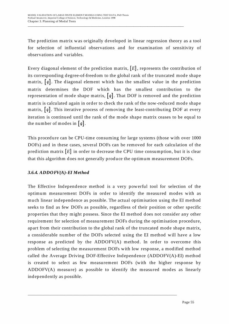
MODEL VALIDATION OF LARGE FINITE ELEMENT MODELS USING TEST DATA, PhD ThesisNedzad Imamovic, Imperial College of Science, Technology & Medicine, London 1998
Chapter 3. Planning of Modal Tests__________________________________________________________________________________________
______________________________________________________________________________________
Page 55
The prediction matrix was originally developed in linear regression theory as a toolfor selection of influential observations and for examination of sensitivity ofobservations and variables.
Every diagonal element of the prediction matrix, E[ ] , represents the contribution of
its corresponding degree-of-freedom to the global rank of the truncated mode shapematrix, φ[ ]. The diagonal element which has the smallest value in the prediction
matrix determines the DOF which has the smallest contribution to therepresentation of mode shape matrix, φ[ ]. That DOF is removed and the prediction
matrix is calculated again in order to check the rank of the now-reduced mode shapematrix, φ[ ]. This iterative process of removing the least-contributing DOF at every
iteration is continued until the rank of the mode shape matrix ceases to be equal tothe number of modes in φ[ ].
This procedure can be CPU-time consuming for large systems (those with over 1000DOFs) and in these cases, several DOFs can be removed for each calculation of theprediction matrix E[ ] in order to decrease the CPU time consumption, but it is clear
that this algorithm does not generally produce the optimum measurement DOFs.
3.6.4. ADDOFV(A)-EI Method
The Effective Independence method is a very powerful tool for selection of theoptimum measurement DOFs in order to identify the measured modes with asmuch linear independence as possible. The actual optimisation using the EI methodseeks to find as few DOFs as possible, regardless of their position or other specificproperties that they might possess. Since the EI method does not consider any otherrequirement for selection of measurement DOFs during the optimisation procedure,apart from their contribution to the global rank of the truncated mode shape matrix,a considerable number of the DOFs selected using the EI method will have a lowresponse as predicted by the ADDOFV(A) method. In order to overcome thisproblem of selecting the measurement DOFs with low response, a modified methodcalled the Average Driving DOF-Effective Independence (ADDOFV(A)-EI) methodis created to select as few measurement DOFs (with the higher response byADDOFV(A) measure) as possible to identify the measured modes as linearlyindependently as possible.
MODEL VALIDATION OF LARGE FINITE ELEMENT MODELS USING TEST DATA, PhD ThesisNedzad Imamovic, Imperial College of Science, Technology & Medicine, London 1998
Chapter 3. Planning of Modal Tests__________________________________________________________________________________________
______________________________________________________________________________________
Page 56
The actual algorithm of the ADDOFV(A)-EI method does not differ very much fromthe algorithm of the basic EI method. The principal goal of the ADDOFV(A)-EImethod is the same as for the EI method, i.e. the truncated mode shape matrix has tobe of full rank. The main difference between the EI and ADDOFV(A)-EI methods isin the selection of the least contributing DOF to the rank of the truncated modeshape matrix, the ADDOFV(A) of all DOFs is taken into consideration in order toremove the DOFs with low response first. This is achieved by multiplication of theADDOFV(A) value of each DOF with the corresponding diagonal values of theprediction matrix, as shown in the expression below:
Eaddofv (a)[ ]NxN
= E[ ]NxN diag ADDOFV( A)[ ]( ) (3.6.4-1)
or eiiaddofv (a) = eii ADDOFV(A)(i) i = 1, N (3.6.4-2)
The optimum measurement DOFs are selected by removing the DOF with thelowest eii
addofv (a) value at each iteration until the rank of the mode shape matrix ceases
to be equal to the number of modes in the mode shape matrix. For large systems(those with 1000 DOFs and over), several DOFs can be removed for each calculationof eii
addofv (a) matrix in order to decrease the CPU-time, but this procedure would
probably produce a different result to the one when only one DOF is removed at atime.
By combining the two methods together, each DOF with a low response value (asdefined by ADDOFV(A) method) would have the chance of removal greatlyincreased compared with the basic EI method so the final selection of measurementDOFs should consist of those with the higher responses.
3.6.5. Application of the EI and ADDOFV(A)-EI Methods
The EI and ADDOFV(A)-EI methods were applied to several test cases and thissection contains results of these studies.
Clamped Disk

MODEL VALIDATION OF LARGE FINITE ELEMENT MODELS USING TEST DATA, PhD ThesisNedzad Imamovic, Imperial College of Science, Technology & Medicine, London 1998
Chapter 3. Planning of Modal Tests__________________________________________________________________________________________
______________________________________________________________________________________
Page 57
A shell model of a disk (shown in Figure 3.6.5-1), which was clamped at the outerradius, was run using MSC/NASTRAN to extract 10 natural frequencies and modeshapes. The number of DOFs of the full model was 1284. The total ADDOFV sum ofall the selected measurement DOFs and the condition number of the truncated modeshape matrix were monitored during the elimination process in order to compareDOF selection for both EI and ADDOFV(A)-EI methods. The higher the value of theADDOFV sum for selected DOFs, the better the selection of measurement DOFsfrom an average response consideration. The smaller the condition number of thetruncated mode shape matrix, the better the selection of measurement DOFs frommode shape linear independence consideration. There are different levels for thecritical condition number defined in the literature, but it will be accepted here that
any value of the condition number below 103 represents a well-conditioned matrix;
the values between 103 and 107 can be considered as poorly conditioned matrix but
are still acceptable in a numerical sense and any value higher than 107 represents a
near-singular or a singular matrix. The values of these two parameters (thecondition number and the ADDOFV sum) have to be balanced to obtain theoptimum selection of measurement DOFs, but there is a priority to keep thecondition number as small as possible compared with the ADDOFV sum forselected measurement DOFs. The values of all these parameters are given in Table3.6.5-1 for different numbers of measurement DOFs.
No. of
measured
DOF
EI
ADDOFV
sum 10−4
ADDOFV-EI
ADDOFV
sum 10−4
EI
Condition
Number
ADDOFV-EI
Condition
Number
EI
Rank
ADDOFV-EI
Rank
100 13.9937 15.3304 1.238 1.704 10 10
50 7.22242 7.55616 1.256 1.694 10 10
30 4.37002 4.47722 1.322 1.675 10 10
20 2.90501 3.05140 1.477 2.03 10 10
15 2.11996 2.30500 1.568 2.233 10 10
10 1.44001 1.47900 2.192 4.527 10 10
Table 3.6.5-1. Clamped disk, 10 Modes, EI and ADDOFV-EI selection ofmeasurement DOF.
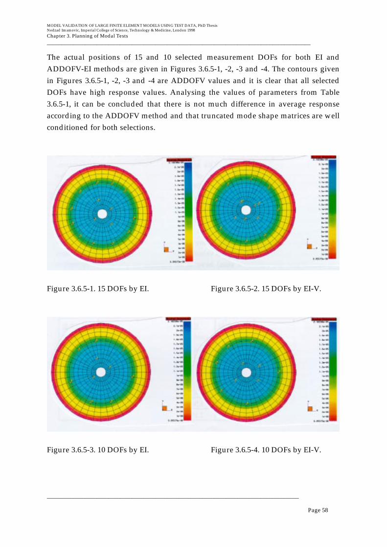
MODEL VALIDATION OF LARGE FINITE ELEMENT MODELS USING TEST DATA, PhD ThesisNedzad Imamovic, Imperial College of Science, Technology & Medicine, London 1998
Chapter 3. Planning of Modal Tests__________________________________________________________________________________________
______________________________________________________________________________________
Page 58
The actual positions of 15 and 10 selected measurement DOFs for both EI andADDOFV-EI methods are given in Figures 3.6.5-1, -2, -3 and -4. The contours givenin Figures 3.6.5-1, -2, -3 and -4 are ADDOFV values and it is clear that all selectedDOFs have high response values. Analysing the values of parameters from Table3.6.5-1, it can be concluded that there is not much difference in average responseaccording to the ADDOFV method and that truncated mode shape matrices are wellconditioned for both selections.
Figure 3.6.5-1. 15 DOFs by EI. Figure 3.6.5-2. 15 DOFs by EI-V.
Figure 3.6.5-3. 10 DOFs by EI. Figure 3.6.5-4. 10 DOFs by EI-V.
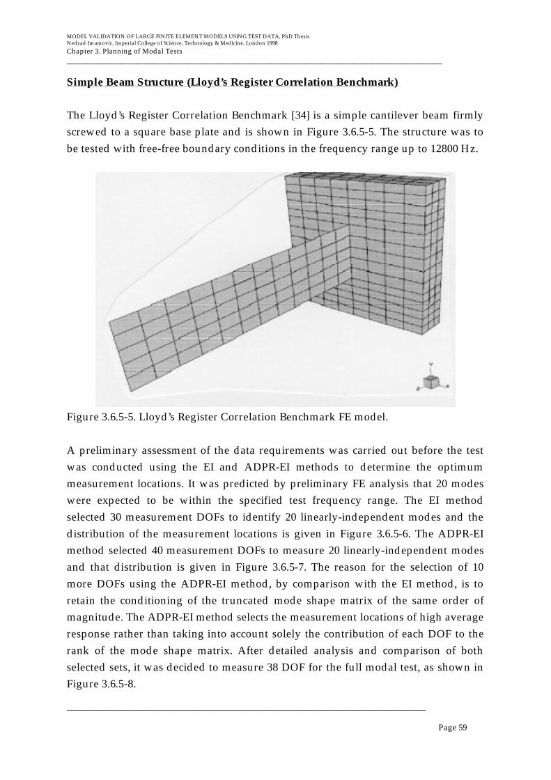
MODEL VALIDATION OF LARGE FINITE ELEMENT MODELS USING TEST DATA, PhD ThesisNedzad Imamovic, Imperial College of Science, Technology & Medicine, London 1998
Chapter 3. Planning of Modal Tests__________________________________________________________________________________________
______________________________________________________________________________________
Page 59
Simple Beam Structure (Lloyd’s Register Correlation Benchmark)
The Lloyd’s Register Correlation Benchmark [34] is a simple cantilever beam firmlyscrewed to a square base plate and is shown in Figure 3.6.5-5. The structure was tobe tested with free-free boundary conditions in the frequency range up to 12800 Hz.
Figure 3.6.5-5. Lloyd’s Register Correlation Benchmark FE model.
A preliminary assessment of the data requirements was carried out before the testwas conducted using the EI and ADPR-EI methods to determine the optimummeasurement locations. It was predicted by preliminary FE analysis that 20 modeswere expected to be within the specified test frequency range. The EI methodselected 30 measurement DOFs to identify 20 linearly-independent modes and thedistribution of the measurement locations is given in Figure 3.6.5-6. The ADPR-EImethod selected 40 measurement DOFs to measure 20 linearly-independent modesand that distribution is given in Figure 3.6.5-7. The reason for the selection of 10more DOFs using the ADPR-EI method, by comparison with the EI method, is toretain the conditioning of the truncated mode shape matrix of the same order ofmagnitude. The ADPR-EI method selects the measurement locations of high averageresponse rather than taking into account solely the contribution of each DOF to therank of the mode shape matrix. After detailed analysis and comparison of bothselected sets, it was decided to measure 38 DOF for the full modal test, as shown inFigure 3.6.5-8.
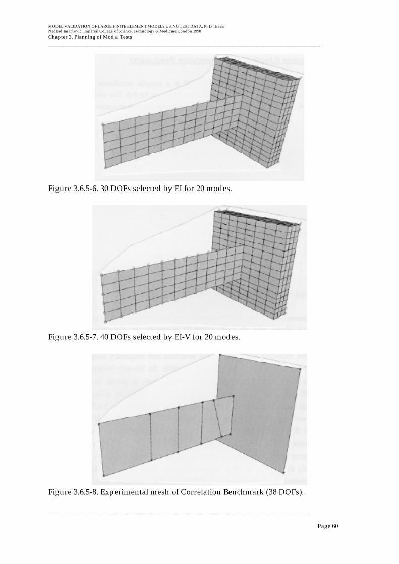
MODEL VALIDATION OF LARGE FINITE ELEMENT MODELS USING TEST DATA, PhD ThesisNedzad Imamovic, Imperial College of Science, Technology & Medicine, London 1998
Chapter 3. Planning of Modal Tests__________________________________________________________________________________________
______________________________________________________________________________________
Page 60
Figure 3.6.5-6. 30 DOFs selected by EI for 20 modes.
Figure 3.6.5-7. 40 DOFs selected by EI-V for 20 modes.
Figure 3.6.5-8. Experimental mesh of Correlation Benchmark (38 DOFs).

MODEL VALIDATION OF LARGE FINITE ELEMENT MODELS USING TEST DATA, PhD ThesisNedzad Imamovic, Imperial College of Science, Technology & Medicine, London 1998
Chapter 3. Planning of Modal Tests__________________________________________________________________________________________
______________________________________________________________________________________
Page 61
Engine Nozzle Structure
The FE model of an engine Nozzle structure and its first several mode shapes areshown in Figure 3.6.5-9. It can be seen that only the few first modes seem to beaccurate due to the quite coarse mesh of the model. Clearly, there is a major problemwhen selecting measurement locations for a structure of such complicated geometry.A complete planning of a modal test was performed for this structure and after theADDOFV-EI method was applied, the obtained measurement locations (shown inFigure 3.6.5-10) seemed quite different from something that engineering intuitionand experience might suggest. Then it was decided to make a set of measurementsat locations obtained by applying ADDOFV-EI (shown in Figure 3.6.5-11) and aseparate set of measurements at locations obtained in consultation withexperimentalists, as shown in Figure 3.6.5-12. After modal analysis was performedon the experimental FRFs - there were about 30 FRFs measured at locations selectedusing ADDOFV-EI and about 72 FRFs measured at locations manually selectedusing intuition and experience - the AUTOMACs on these separate data sets werecalculated. It can be seen quite clearly that the smallest off-diagonal values in theAUTOMAC table is achieved using a data set at locations selected by the ADDOFV-EI method as shown in Figure 3.6.5-13. The AUTOMAC table obtained using dataset at locations selected manually clearly indicates that some modes were notidentified properly and that an aliasing problem is present, as shown in Figure 3.6.5-14. This example demonstrates the effectiveness of this new combined method eventhough the initial data used for these calculations were of limited accuracy. It shouldbe noted that ADDOFV coefficient was used in the selection procedure since themeasurements were performed by a laser vibrometer which measures velocity at thesurface locations.

MODEL VALIDATION OF LARGE FINITE ELEMENT MODELS USING TEST DATA, PhD ThesisNedzad Imamovic, Imperial College of Science, Technology & Medicine, London 1998
Chapter 3. Planning of Modal Tests__________________________________________________________________________________________
______________________________________________________________________________________
Page 62
Figure 3.6.5-9. Mode shape contours of engine Nozzle Structure.

MODEL VALIDATION OF LARGE FINITE ELEMENT MODELS USING TEST DATA, PhD ThesisNedzad Imamovic, Imperial College of Science, Technology & Medicine, London 1998
Chapter 3. Planning of Modal Tests__________________________________________________________________________________________
______________________________________________________________________________________
Page 63
Figure 3.6.5-10. 30 DOFs selected by EI-V for 12 modes.
Figure 3.6.5-11. Measurements on engine Nozzle using laser vibrometer.
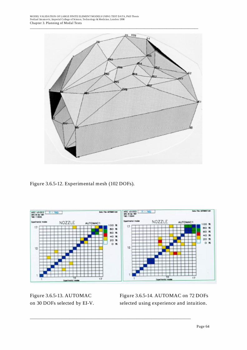
MODEL VALIDATION OF LARGE FINITE ELEMENT MODELS USING TEST DATA, PhD ThesisNedzad Imamovic, Imperial College of Science, Technology & Medicine, London 1998
Chapter 3. Planning of Modal Tests__________________________________________________________________________________________
______________________________________________________________________________________
Page 64
Figure 3.6.5-12. Experimental mesh (102 DOFs).
Figure 3.6.5-13. AUTOMAC Figure 3.6.5-14. AUTOMAC on 72 DOFson 30 DOFs selected by EI-V. selected using experience and intuition.
MODEL VALIDATION OF LARGE FINITE ELEMENT MODELS USING TEST DATA, PhD ThesisNedzad Imamovic, Imperial College of Science, Technology & Medicine, London 1998
Chapter 3. Planning of Modal Tests__________________________________________________________________________________________
______________________________________________________________________________________
Page 65
3.6.6. Conclusions for Selection of Optimum Measurement Locations
Two useful and efficient techniques for the automatic selection of optimummeasurement DOFs have been presented. The EI method was used as a base todevelop a new technique, the “combined ADDOFV(A)-EI method”, whichautomatically have been measurement locations of high average response. Bothtechniques were applied to a few test cases and the results obtained demonstratedthe capabilities of the methods. The major weakness of the basic EI method is that itcan include in the selection some DOFs which have low values of the averageresponse (locations close to or on nodal lines), but as a result, the EI method can beused to select a smaller number of measurement DOFs than the ADDOFV(A)-EImethod, which also takes into consideration the values of the average responses ofthe potential measurement locations.
In order to use both techniques properly, it is recommended that the selection ofmeasurement DOFs obtained by the ADDOFV(A)-EI method be used but thatdouble the number of measurement DOFs (compared with the number of modes tobe measured) should be selected. Following this logic of modal test planning, moreaccurate FRFs should be measured, but the conditioning of the truncated modeshape matrix should be in line with the value obtained by the EI method selectionsince more measurement DOFs are selected.
3.7. Reliability of Pre-Test Planning: Why/When does it work?
In order to plan a modal test successfully, it is necessary to know the frequencyrange in which measurements need to be performed and this information isdetermined from the relationship between the frequency-domain and the final time-domain analysis, as discussed in Chapter 2. Also, this analysis requires knowledgeof natural frequencies and mode shapes of a structure and this requirement poses amajor threat to the accuracy and reliability of pre-test planning. Analysts who wishto use these techniques have to be aware of limitations of the pre-test planning interms of its accuracy and reliability.
It has been demonstrated on a few practical examples using real experimental datathat pre-test planning can work and does work if used sensibly and according therules described in this chapter. The Nozzle example demonstrates that even ifpreliminary predictions of the FE model are not particularly accurate, pre-test

MODEL VALIDATION OF LARGE FINITE ELEMENT MODELS USING TEST DATA, PhD ThesisNedzad Imamovic, Imperial College of Science, Technology & Medicine, London 1998
Chapter 3. Planning of Modal Tests__________________________________________________________________________________________
______________________________________________________________________________________
Page 66
planning will still produce some sensible answers for the optimum suspension,excitation and measurement positions. The real question is how much pre-testplanning is really dependent on the accuracy of the preliminary data?
A major strength of all pre-test planning techniques lies in their simplicity ofmathematical formulation. These techniques use neither the spatial or responseproperties of the structure, they use only the modal properties (the naturalfrequencies and mode shapes), and the importance of the natural frequencies can beneglected by comparison with mode shapes. All pre-test planning techniques assesspositions of nodal lines for the selected modes. Methods for determination of theoptimum suspension and excitation positions use all the modes averaged, ratherthan as individual properties and that is the major strength of these techniques.Experience shows that preliminary predictions tend to have higher accuracy for themode shapes rather than for the natural frequencies.
For instance, for a simple cantilever beam such as the Lloyd’s Register structure thatis clamped at one end, the predicted mode shapes will be several pure bending andtorsional modes. However, since the structure has a quite crude connection at thebase plate, it is unlikely that the connection is completely symmetrical andconsequently the mode shapes will not be pure bendings and torsions. In fact, a verydetailed modal analysis shows that the actual mode shapes of the structure arecombinations of bending and torsions.
Since the pre-test planning techniques use the mode shapes averaged rather thanindividually, even if the predicted mode shapes are not distributed very accuratelyby comparison with the actual mode shapes, the average information should have ahigher degree of accuracy than the individual modes. This is a major reason for anenhanced reliability and accuracy of the pre-test planning. Also, experience showsthat distribution of mode shapes is dependent on stiffness and mass, but it is moredependent on the geometry of the model, and since in most practical situations thegeometry is known quite accurately, there is a high probability that most sensiblemodels produce a sensible averaged information that can be used in the pre-testplanning.

MODEL VALIDATION OF LARGE FINITE ELEMENT MODELS USING TEST DATA, PhD ThesisNedzad Imamovic, Imperial College of Science, Technology & Medicine, London 1998
Chapter 3. Planning of Modal Tests__________________________________________________________________________________________
______________________________________________________________________________________
Page 67
3.8. Closing Remarks
This chapter has presented a number of new techniques for the planning of modaltests. These techniques are designed in such a way that the level of accuracyrequired of the preliminary data used for predictions is minimised. There are severaldifferent conditions for a more reliable modal test: the optimum suspension,excitation and measurement positions. Data requirements are incorporated into theoverall strategy for pre-test planning but this topic will be discussed further in thefollowing sections. It has been demonstrated on several real engineering structuresthat these techniques can be used as a valuable tool for planning of modal tests.

MODEL VALIDATION OF LARGE FINITE ELEMENT MODELS USING TEST DATA, PhD ThesisNedzad Imamovic, Imperial College of Science, Technology & Medicine, London 1998
Chapter 4. Model Correlation__________________________________________________________________________________________
______________________________________________________________________________________
Page 68
4.0 Model Correlation
4.1. Introduction
This chapter presents the basis for an automatic correlation algorithm for structuraldynamic models, which can be used during a model updating procedure in order topair matching experimental and theoretical model CMPs (correlated mode pairs)automatically. Also, a method of modal complexity assessment is presented.Evaluation of modal complexity of experimental modes is a useful check onexperimental data in order to assess consistency of the data. A new criterion formode shape comparison (SCO) is introduced. The method is based on the SEREPreduction method and does not require any additional data to the naturalfrequencies and modes from theoretical model.
In addition, this chapter presents a new method for the determination of thenumber of modes required for accurate regeneration of FRFs using the modalsummation approach. Theoretical FRFs are rarely computed by direct inversion ofthe dynamic stiffness matrix because of the CPU requirements for this calculation.Instead, they are regenerated using the modal summation approach, including onlya limited number of modes and simply neglecting the influence of the highermodes. Using the modal FRF regeneration approach, the analyst always faces thequestion: "How many modes should be included for the FRF regenerationsummation in order to minimise the influence of omitted higher modes?". Thischapter presents a new method which provides an answer to this question.
4.2. Standard Correlation Methods
Validation of theoretical structural dynamic models is usually performed bycomparison of theoretically-predicted with experimentally measured dynamiccharacteristics of structures. When a successful modal test of a structure iscompleted, correlation between theoretical and experimental sets of data isundertaken and if the agreement is satisfactory, the theoretical model of thestructure is validated and considered to be suitable for use in further analysis(transient response, assembled structure analysis, fluid-structure interactionanalysis, etc.). However, if satisfactory agreement is not obtained, then somemodifications must be made to the theoretical model in order to improve correlationwith the corresponding experimental results. This model correlation consists of

MODEL VALIDATION OF LARGE FINITE ELEMENT MODELS USING TEST DATA, PhD ThesisNedzad Imamovic, Imperial College of Science, Technology & Medicine, London 1998
Chapter 4. Model Correlation__________________________________________________________________________________________
______________________________________________________________________________________
Page 69
mode shape pairing between theoretical and experimental data sets and comparisonof the values of corresponding natural frequencies and mode shapes.
Theoretical and experimental sets of modal data consist of a number of naturalfrequencies and mode shapes on the corresponding meshes for each model. A majorpractical problem in the correlation process is the incompatibility between these twomeshes resulting from the experimental data set incompleteness, i.e. the limitednumber of measurement points in a limited measured frequency range.
Generally, assessment of the degree of correlation between two sets of data isperformed both numerically and visually.
4.2.1. Numerical Comparison of Mode Shapes
Numerical comparison between two sets of modal data consists of the calculation ofdifferent correlation coefficients which give quantitative values of similaritiesbetween two mode shapes. All numerical correlation methods use the orthogonalityproperties of mode shapes in order to exploit the differences between them. Themost commonly-used one for indication of CMPs is the MAC (Modal AssuranceCriterion) [7], which calculates the least-squares deviation about a straight line ofthe plot of two arbitrarily-scaled mode shapes, and the NCO (Normalised Cross-Orthogonality) [8], which is basically the MAC coefficient weighted by a partitionedglobal mass or stiffness matrix. A good correlation between two modes is observedfor MAC and NCO values close to 1 and a poor correlation corresponds to valuesclose to zero. Since mode shapes are orthogonal with respect to the full mass orstiffness matrix, and the measured set of DOFs is never complete, it is impossible tospecify absolute limits for indication of good or poor correlation based on the MACor NCO correlation coefficients.
MAC i, j( )=ψX{ }
i
T ψ A{ }j
* 2
ψ X{ }i
T ψ X{ }i
*. ψA{ }j
T ψ A{ }j
* (4.2.1-1)
NCO i, j( )=ψX{ }
i
TMA[ ] ψA{ }
j
* 2
ψ X{ }i
TMA[ ] ψ X{ }i
*. ψ A{ }j
TMA[ ] ψ A{ }j
* (4.2.1-2)

MODEL VALIDATION OF LARGE FINITE ELEMENT MODELS USING TEST DATA, PhD ThesisNedzad Imamovic, Imperial College of Science, Technology & Medicine, London 1998
Chapter 4. Model Correlation__________________________________________________________________________________________
______________________________________________________________________________________
Page 70
Other correlation coefficients which are used in practice include the slope of the beststraight line through the points of the plot of two identically-scaled mode shapes;the MSF (Modal Scale Factor) [2].
MSF i, j( )=φX{ }
i
T φA{ }j
*
φ A{ }j
T φ A{ }j
* (4.2.1-3)
4.2.2. Visual Comparison of Mode Shapes
Visual comparison between two sets of modal data includes a process whichinvolves the analyst’s non-quantitative visual assessment of any kind of graphically-presented data. It usually consists of simultaneous animation of one mode shapefrom each of the two sets and direct comparison of their natural frequencies. Thismethod basically consists of a visual comparison of the patterns of two differentmode shapes and a non-quantitative analyst assessment of differences or similaritiesbetween two mode shape patterns. A problem arises when one experimental modeappears to match two or more theoretical modes. Although this can happen forseveral reasons, as will be discussed later, a more detailed inspection is necessary inorder to identify the CMPs.
It is important to stress here that during this process the analyst comparesexperimental and theoretical meshes too and, to some extent, the analyst usesadditional information about the structure in connection with the experimentalmesh. This additional information includes the geometry of the structure which isalready known to the analyst. A good example of this is a very coarse experimentalmesh of an aircraft engine casing, which hardly resembles an approximation to theshape of the engine itself. During the animation comparison process, the analystuses his/her prior knowledge of the geometrical shape of a structure which isvisually assigned to the experimental mesh of the structure. It is interesting thatvisual linearisation for the points on the mesh is assumed as true as it is viewed onthe screen, but which is generally unknown, because it was not measured. This iswhere some extra information about the experimental mode shapes can beintroduced, and can disrupt the visual pattern comparison for geometricallycomplex mode shapes.
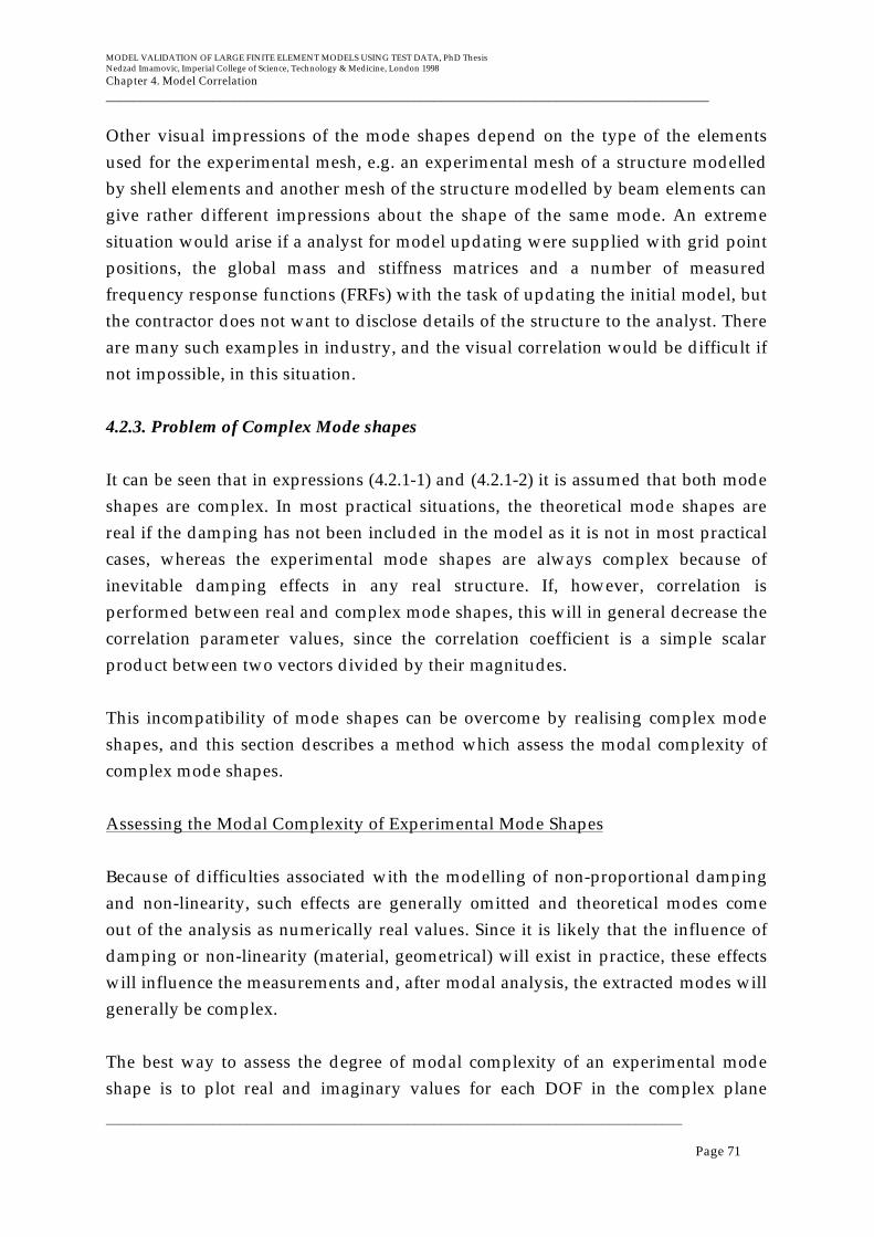
MODEL VALIDATION OF LARGE FINITE ELEMENT MODELS USING TEST DATA, PhD ThesisNedzad Imamovic, Imperial College of Science, Technology & Medicine, London 1998
Chapter 4. Model Correlation__________________________________________________________________________________________
______________________________________________________________________________________
Page 71
Other visual impressions of the mode shapes depend on the type of the elementsused for the experimental mesh, e.g. an experimental mesh of a structure modelledby shell elements and another mesh of the structure modelled by beam elements cangive rather different impressions about the shape of the same mode. An extremesituation would arise if a analyst for model updating were supplied with grid pointpositions, the global mass and stiffness matrices and a number of measuredfrequency response functions (FRFs) with the task of updating the initial model, butthe contractor does not want to disclose details of the structure to the analyst. Thereare many such examples in industry, and the visual correlation would be difficult ifnot impossible, in this situation.
4.2.3. Problem of Complex Mode shapes
It can be seen that in expressions (4.2.1-1) and (4.2.1-2) it is assumed that both modeshapes are complex. In most practical situations, the theoretical mode shapes arereal if the damping has not been included in the model as it is not in most practicalcases, whereas the experimental mode shapes are always complex because ofinevitable damping effects in any real structure. If, however, correlation isperformed between real and complex mode shapes, this will in general decrease thecorrelation parameter values, since the correlation coefficient is a simple scalarproduct between two vectors divided by their magnitudes.
This incompatibility of mode shapes can be overcome by realising complex modeshapes, and this section describes a method which assess the modal complexity ofcomplex mode shapes.
Assessing the Modal Complexity of Experimental Mode Shapes
Because of difficulties associated with the modelling of non-proportional dampingand non-linearity, such effects are generally omitted and theoretical modes comeout of the analysis as numerically real values. Since it is likely that the influence ofdamping or non-linearity (material, geometrical) will exist in practice, these effectswill influence the measurements and, after modal analysis, the extracted modes willgenerally be complex.
The best way to assess the degree of modal complexity of an experimental modeshape is to plot real and imaginary values for each DOF in the complex plane
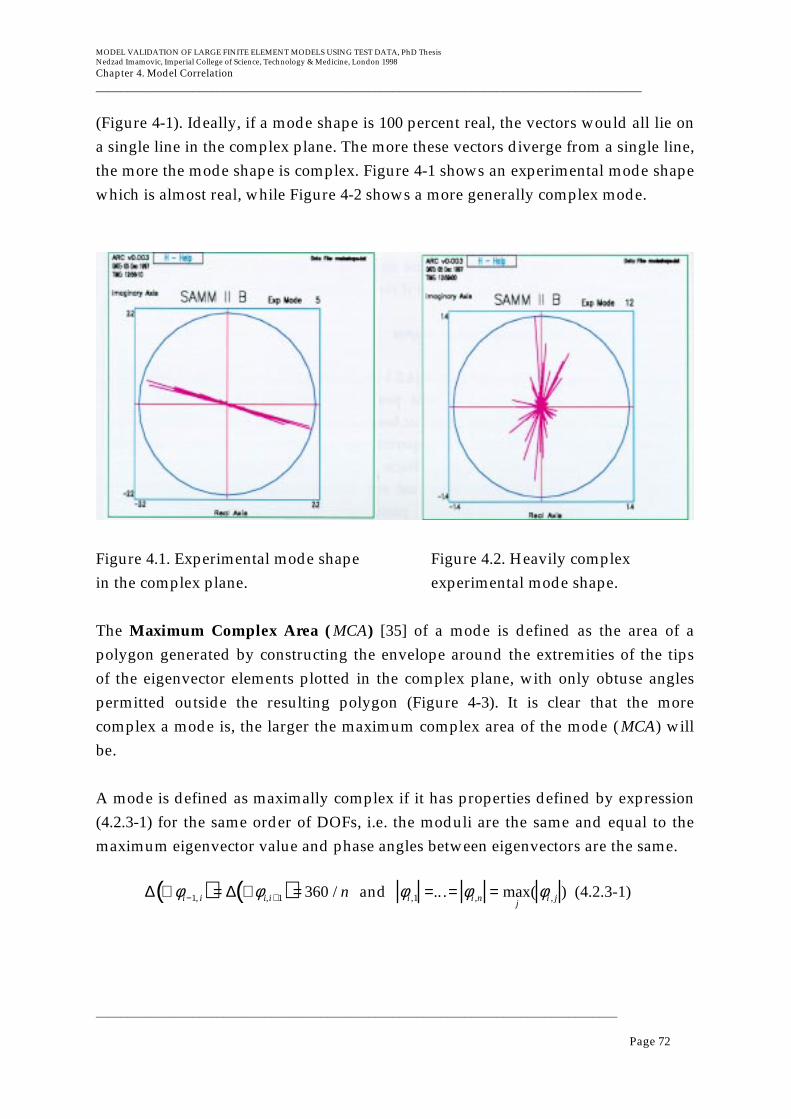
MODEL VALIDATION OF LARGE FINITE ELEMENT MODELS USING TEST DATA, PhD ThesisNedzad Imamovic, Imperial College of Science, Technology & Medicine, London 1998
Chapter 4. Model Correlation__________________________________________________________________________________________
______________________________________________________________________________________
Page 72
(Figure 4-1). Ideally, if a mode shape is 100 percent real, the vectors would all lie ona single line in the complex plane. The more these vectors diverge from a single line,the more the mode shape is complex. Figure 4-1 shows an experimental mode shapewhich is almost real, while Figure 4-2 shows a more generally complex mode.
Figure 4.1. Experimental mode shape Figure 4.2. Heavily complexin the complex plane. experimental mode shape.
The Maximum Complex Area ( MCA) [35] of a mode is defined as the area of apolygon generated by constructing the envelope around the extremities of the tipsof the eigenvector elements plotted in the complex plane, with only obtuse anglespermitted outside the resulting polygon (Figure 4-3). It is clear that the morecomplex a mode is, the larger the maximum complex area of the mode ( MCA) willbe.
A mode is defined as maximally complex if it has properties defined by expression(4.2.3-1) for the same order of DOFs, i.e. the moduli are the same and equal to themaximum eigenvector value and phase angles between eigenvectors are the same.
∆ ∠φi −1, i( )= ∆ ∠φ i,i +1( )= 360 / n and φi ,1 =.. .= φi ,n = maxj
( φi , j ) (4.2.3-1)
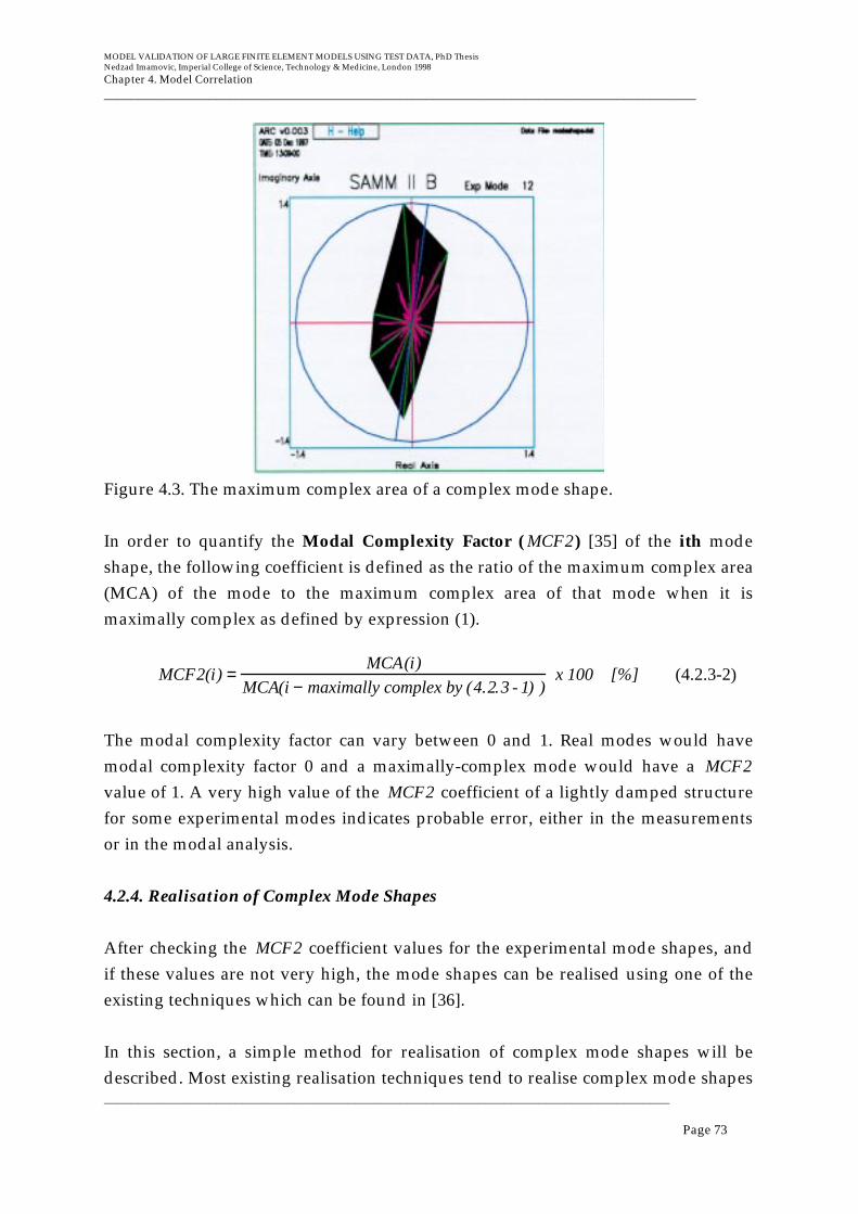
MODEL VALIDATION OF LARGE FINITE ELEMENT MODELS USING TEST DATA, PhD ThesisNedzad Imamovic, Imperial College of Science, Technology & Medicine, London 1998
Chapter 4. Model Correlation__________________________________________________________________________________________
______________________________________________________________________________________
Page 73
Figure 4.3. The maximum complex area of a complex mode shape.
In order to quantify the Modal Complexity Factor ( MCF2) [35] of the ith modeshape, the following coefficient is defined as the ratio of the maximum complex area(MCA) of the mode to the maximum complex area of that mode when it ismaximally complex as defined by expression (1).
MCF2(i) =MCA(i)
MCA(i − maximally complex by (4.2.3 - 1) )x 100 [%] (4.2.3-2)
The modal complexity factor can vary between 0 and 1. Real modes would havemodal complexity factor 0 and a maximally-complex mode would have a MCF2
value of 1. A very high value of the MCF2 coefficient of a lightly damped structurefor some experimental modes indicates probable error, either in the measurementsor in the modal analysis.
4.2.4. Realisation of Complex Mode Shapes
After checking the MCF2 coefficient values for the experimental mode shapes, andif these values are not very high, the mode shapes can be realised using one of theexisting techniques which can be found in [36].
In this section, a simple method for realisation of complex mode shapes will bedescribed. Most existing realisation techniques tend to realise complex mode shapes

MODEL VALIDATION OF LARGE FINITE ELEMENT MODELS USING TEST DATA, PhD ThesisNedzad Imamovic, Imperial College of Science, Technology & Medicine, London 1998
Chapter 4. Model Correlation__________________________________________________________________________________________
______________________________________________________________________________________
Page 74
in such a way that the correlation between complex and the corresponding realmode shapes is retained as high as possible. Generally, this approach is notrecommended here since this assumes that there is a fair correlation between theexperimental and theoretical modes and that the correlated mode pairs are known,what may not be the case. Another reason for questioning these approaches is thatthey tune the experimental mode shapes to the corresponding theoretical modeshapes (if these are known at that stage), but these theoretical mode shapes may notbe completely accurate (that is why the correlation and updating are beingperformed in the first place). Hence, these approaches are essentially based on someassumptions that are incompatible with model validation technology and thereforeare not recommended to be used in the application of model validation.
An extremely simple approach for realisation of complex modes will be describedhere. The most important feature of this realisation method is that there is noreference to any theoretical data in the realisation process. A lightly-damped and acomplex mode shape is shown in Figure 4-2. In order to realise this complex modeshape it is necessary to ensure that the maximum possible values of complex modalparameters are retained when the mode shape is realised. The realisation processinvolves projecting complex plane modal parameter vectors of each DOF to acommon single straight line. It is then necessary to find the angle of the line whichwould have a maximum value of the sum of all projections of modal parameters tothat line. This problem can be solved by simple optimisation of projected value to asingle line as a function of the angle of that line. Applying this procedure, it ispossible that some modal parameters are perpendicular to the realisation line, andtherefore their contribution to the mode shape would be completely lost. This is amajor reason for optimising the value of the lengths of modal parameters duringrealisation process, since this will ensure that most contributing modal parametersare least distorted. All DOFs that have small modal parameter values are lessimportant in the realisation process because the accuracy of modal parameters isapproximately proportional to their values. A heavily complex mode shape and itsrealisation line are shown in Figure 4-3.
There is no realisation process that can retain all the properties of a complex modeshape; they all distort and cause some inaccuracies in the realised mode shapes. Theeffects of the realisation process are dependent on the technique used, but the majoradvantage of the realisation approach presented here is that these distortions of
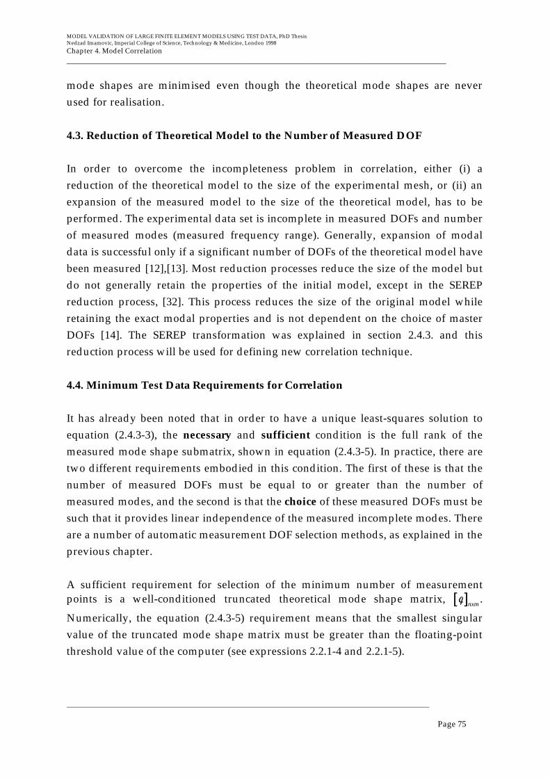
MODEL VALIDATION OF LARGE FINITE ELEMENT MODELS USING TEST DATA, PhD ThesisNedzad Imamovic, Imperial College of Science, Technology & Medicine, London 1998
Chapter 4. Model Correlation__________________________________________________________________________________________
______________________________________________________________________________________
Page 75
mode shapes are minimised even though the theoretical mode shapes are neverused for realisation.
4.3. Reduction of Theoretical Model to the Number of Measured DOF
In order to overcome the incompleteness problem in correlation, either (i) areduction of the theoretical model to the size of the experimental mesh, or (ii) anexpansion of the measured model to the size of the theoretical model, has to beperformed. The experimental data set is incomplete in measured DOFs and numberof measured modes (measured frequency range). Generally, expansion of modaldata is successful only if a significant number of DOFs of the theoretical model havebeen measured [12],[13]. Most reduction processes reduce the size of the model butdo not generally retain the properties of the initial model, except in the SEREPreduction process, [32]. This process reduces the size of the original model whileretaining the exact modal properties and is not dependent on the choice of masterDOFs [14]. The SEREP transformation was explained in section 2.4.3. and thisreduction process will be used for defining new correlation technique.
4.4. Minimum Test Data Requirements for Correlation
It has already been noted that in order to have a unique least-squares solution toequation (2.4.3-3), the necessary and sufficient condition is the full rank of themeasured mode shape submatrix, shown in equation (2.4.3-5). In practice, there aretwo different requirements embodied in this condition. The first of these is that thenumber of measured DOFs must be equal to or greater than the number ofmeasured modes, and the second is that the choice of these measured DOFs must besuch that it provides linear independence of the measured incomplete modes. Thereare a number of automatic measurement DOF selection methods, as explained in theprevious chapter.
A sufficient requirement for selection of the minimum number of measurementpoints is a well-conditioned truncated theoretical mode shape matrix, φ[ ]nxm
.
Numerically, the equation (2.4.3-5) requirement means that the smallest singularvalue of the truncated mode shape matrix must be greater than the floating-pointthreshold value of the computer (see expressions 2.2.1-4 and 2.2.1-5).

MODEL VALIDATION OF LARGE FINITE ELEMENT MODELS USING TEST DATA, PhD ThesisNedzad Imamovic, Imperial College of Science, Technology & Medicine, London 1998
Chapter 4. Model Correlation__________________________________________________________________________________________
______________________________________________________________________________________
Page 76
Another type of check is an assessment of the ratio of the largest to the smallestsingular values (condition number) of the theoretical mode shape matrix φ[ ]nxm
as
explained in section 3.6.5. The larger the ratio, the worse the choice of themeasurement DOFs.
4.5. SEREP-based Normalised Cross Orthogonality Correlation Technique
The Modal Assurance Criterion (MAC) is the most commonly-used correlationcoefficient for assessing linear (in)dependence of mode shapes. However, thistechnique has been found inappropriate for some applications, and a SEREPtheoretical mass reduced cross-orthogonality (SCO) correlation coefficient, asdefined in equation (4.5-1), can be used instead [37].
SCO i, j( ) =ψ X ,i{ }
n
T( φA[ ]
nxm
+T φA[ ]mxn
+) ψ A, j{ }
n
* 2
ψ X ,i{ }n
T( φA[ ]
nxm
+T φ A[ ]mxn
+) ψ X ,i{ }
n
*. ψ A, j{ }
n
T( φA[ ]
nxm
+ T φA[ ]mxn
+) ψ A , j{ }
n
* (4.5-1)
It is possible to use either a SEREP mass or stiffness reduced matrix from equations(2.4.3-10) or (2.4.3-11), based on experimental rather than theoretical modal data,but since the measurement accuracy for experimental mode shapes is generally nothigh (the experimental modes contain noise and that makes solution of equation(2.4.3-4) ill-conditioned), and because the theoretical mass matrix is usually knownmore accurately than the theoretical stiffness matrix, the most appropriate solutionfor SEREP-based correlation coefficient is to use only the theoretical mode shapes asgiven in equation (4.5-1).
This correlation coefficient has an advantage over the MAC in that it is moresensitive to the actual similarity or dissimilarity between the mode shapes. TheSEREP mass matrix reduced normalised Cross Orthogonality (SCO) correlationcoefficient will generally have a higher value for two similar mode shapes than theMAC correlation coefficient, and conversely for two dissimilar mode shapes, SCOwill have a lower value than MAC. Another interesting feature of the SCOcorrelation coefficient is that no actual theoretical mass or stiffness matrices arerequired, i.e. no extra data are required other than those used for the standard MACcalculation.

MODEL VALIDATION OF LARGE FINITE ELEMENT MODELS USING TEST DATA, PhD ThesisNedzad Imamovic, Imperial College of Science, Technology & Medicine, London 1998
Chapter 4. Model Correlation__________________________________________________________________________________________
______________________________________________________________________________________
Page 77
Although realisation of complex mode shapes is proposed in the correlationprocedure, SCO can handle complex modes. It should be noted here that in somecases of comparison of real and complex modes, the correlation results can changewhen realised complex mode shapes are used rather than original complex modeshapes. The influence of realisation process on the correlation results is limited inmost practical test cases, although it is recommended to check the correlation resultsboth before and after the realisation process.
4.6. Natural Frequency Comparison
Comparison of the natural frequencies between two models is usually performed byfitting the best straight line through a plot of the natural frequency points. Thiscomparison technique cannot help to select the CMPs, and so a new technique thatcan be used for selection of CMPs is proposed here.
A Natural Frequency Difference (NFD) correlation coefficient gives an assessmentof the differences between all combinations of natural frequencies, i.e. all potentialCMPs.
NFD(i, j) =ω i − ω j
min(ω i ,ω j)x 100 [%] (4.6-1)
A typical plot of the NFD matrix is given in Figure 4-4. It is important to note thatthis correlation coefficient should be used only as an additional piece of informationwhen selecting CMPs, and not as the sole indicator. The larger the NFD value fortwo mode shapes is, the less likely the pair is to be a CMP.
Figure 4.4. Natural Frequency Difference table.
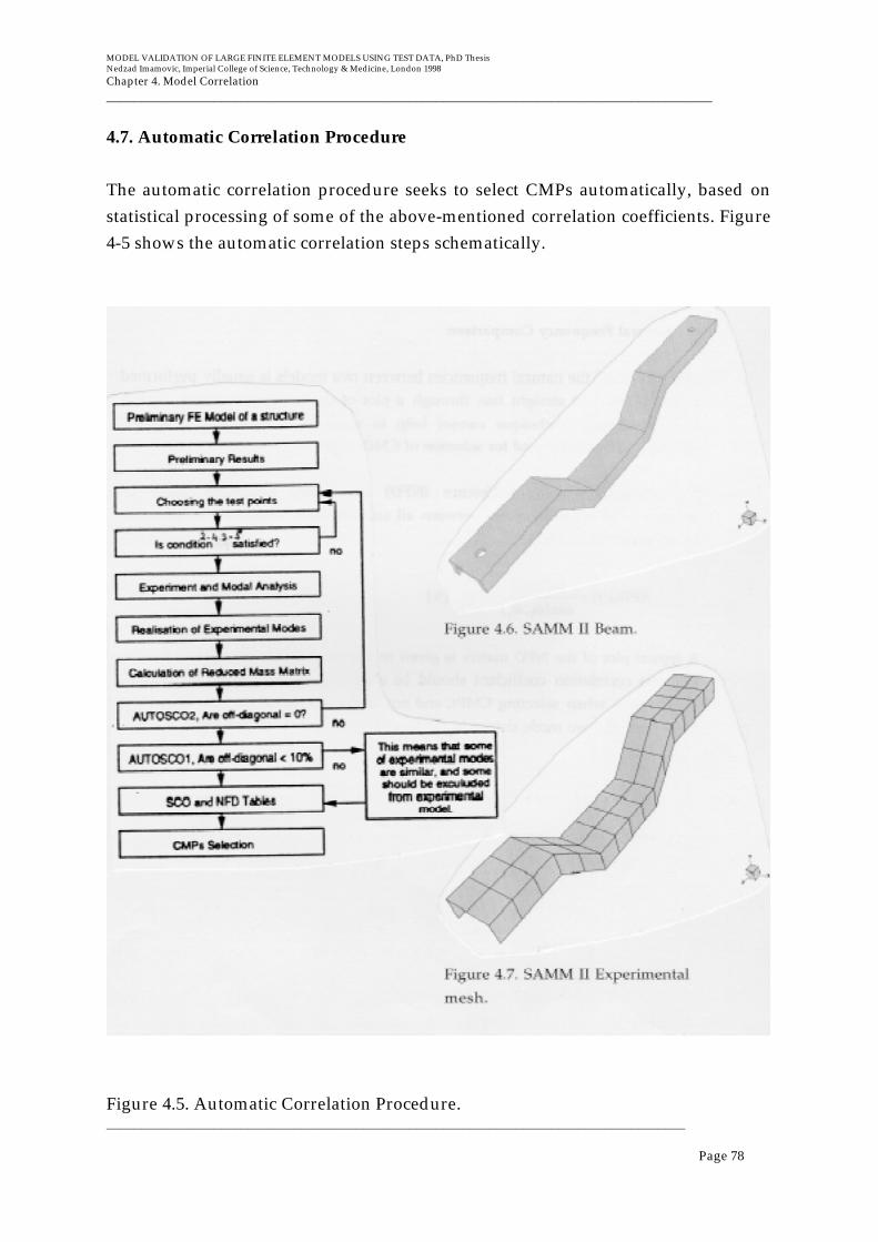
MODEL VALIDATION OF LARGE FINITE ELEMENT MODELS USING TEST DATA, PhD ThesisNedzad Imamovic, Imperial College of Science, Technology & Medicine, London 1998
Chapter 4. Model Correlation__________________________________________________________________________________________
______________________________________________________________________________________
Page 78
4.7. Automatic Correlation Procedure
The automatic correlation procedure seeks to select CMPs automatically, based onstatistical processing of some of the above-mentioned correlation coefficients. Figure4-5 shows the automatic correlation steps schematically.
Figure 4.5. Automatic Correlation Procedure.
MODEL VALIDATION OF LARGE FINITE ELEMENT MODELS USING TEST DATA, PhD ThesisNedzad Imamovic, Imperial College of Science, Technology & Medicine, London 1998
Chapter 4. Model Correlation__________________________________________________________________________________________
______________________________________________________________________________________
Page 79
The procedure begins with the planning of a modal test on the structure. The firststep is to generate a model of the structure and to extract the eigensolution in therequired frequency range. Then, using any of the existing measurement pointselection methods, the minimum data requirements can be established, i.e. thenumber of measured DOFs has to be greater than the number of measured modes,and the rank of the reduced mode shape matrix - determined by particular choice ofDOFs - must be equal to the number of measured modes.
The second step in the algorithm is realisation of complex experimental modeshapes. In section 4.2.3 it was shown how to assess the complexity of the measuredmode shapes. Generally, for a structure which is not very heavily damped, themodal complexity factor should not be very high. It is difficult to set a limit forcritical modal complexity, but if the value of this coefficient is very high for somemodes, those should be plotted in the complex plane and checked (Figures 4-1, 4-2and 4-3). This checking is actually part of the modal analysis procedure and gives ageneral assessment of the reliability of the measured modal data. After this check,the experimental mode shapes should be realised using the techniques given insection 4.2.4, taking care to note that any realisation process is approximate.
The third step in this algorithm is the auto correlation of theoretical data on theequivalent experimental mesh in order to assess the independence of the theoreticalmode shapes. Auto (self) correlation of theoretical mode shape data using the SCOformulation will give a perfect correlation result: all diagonal terms are 1 and all off-diagonal terms are zero (Figure 4-8(d)). The reason for this is that because of thenormalisation of the mode shapes by the SEREP-reduced mass matrix, and becausethese mode shapes are orthogonal since they come from theoretical analysis, aperfect check is obtained and this diagram shows how the actual correlation pictureshould ideally be if the experimental mode shapes are exactly equivalent to thecorresponding theoretical ones. Additionally, an auto correlation of the theoreticalmode shapes, but confined to the DOFs corresponding to the experimental mesh,using the MAC correlation coefficient can be performed in order to assess theperformance of the minimum test data requirement procedure which was used inthe pre-test phase.
The fourth step in the algorithm is an auto correlation of the experimental modeshapes using the SCO correlation check in order to assess the independence of theexperimental mode shapes. Ideally, the resulting SCO matrix should have all off-
MODEL VALIDATION OF LARGE FINITE ELEMENT MODELS USING TEST DATA, PhD ThesisNedzad Imamovic, Imperial College of Science, Technology & Medicine, London 1998
Chapter 4. Model Correlation__________________________________________________________________________________________
______________________________________________________________________________________
Page 80
diagonal terms identically zero. If any of the off-diagonal terms in the SCO matrixare not zero, this will indicate a linear dependence or similarity between thecorresponding pair of modes. In most cases, the reason for this is either an error inthe modal analysis which occurred during the modal parameter extraction processor because there are not enough measured DOFs. If it was found that some ofmodes in the experimental model were "generated" by the modal analysisprocedure, these modes should be deleted from the experimental set. The secondreason should not normally occur if the test data requirements were plannedappropriately according to step 1.
The fifth step in the algorithm is the preliminary selection of CMPs which is basedon the SEREP Cross Orthogonality (SCO). In the case of an ideal correlation, someterms of the SCO matrix should be equal to 1 and the rest of the matrix terms shouldbe equal to zero, indicating perfect mode pairing. Because of discrepancies betweentheoretical and experimental models, high values in the SCO matrix indicate goodagreement and low values indicate poor agreement between mode shapes.Generally, the SCO matrix will be similar to the MAC matrix with the improvementthat the similarity between two modes will be represented with the higher SCOvalues than the MAC values, and dissimilarity between mode shapes will berepresented with the lower SCO values than the MAC values, as explained insection 4.5.
The last step in the algorithm is the final selection of the CMPs using both SCO andNFD correlation tables. The SCO table is scanned first and if there are anyuncertainties about the selection of particular CMPs, the NFD table is used in orderto clarify the possibility of those CMPs. Generally, any two modes whose NFDvalue is greater than 100 % should not be taken as a possible CMP.
4.8. Test Case Study
The SAMM II B structure (shown in Figure 4-6) was used to demonstrate the use ofthe automatic correlation procedure. The measurements were performed at the 105DOFs on the mesh shown in Figure 4-7. The minimum test data requirement, i.e.condition (2.4.3-5), is satisfied and the SEREP reduction process is well-conditioned,checking the singular values of reduced mode shape matrix φA[ ]nxm
.
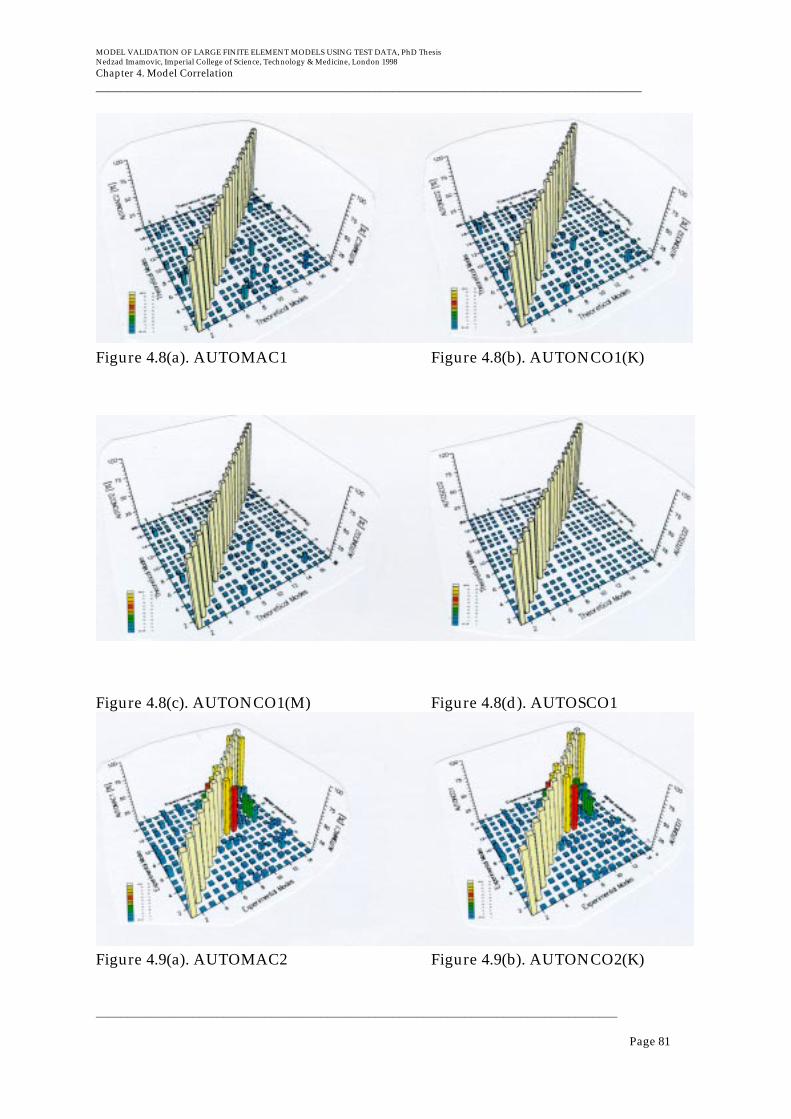
MODEL VALIDATION OF LARGE FINITE ELEMENT MODELS USING TEST DATA, PhD ThesisNedzad Imamovic, Imperial College of Science, Technology & Medicine, London 1998
Chapter 4. Model Correlation__________________________________________________________________________________________
______________________________________________________________________________________
Page 81
Figure 4.8(a). AUTOMAC1 Figure 4.8(b). AUTONCO1(K)
Figure 4.8(c). AUTONCO1(M) Figure 4.8(d). AUTOSCO1
Figure 4.9(a). AUTOMAC2 Figure 4.9(b). AUTONCO2(K)

MODEL VALIDATION OF LARGE FINITE ELEMENT MODELS USING TEST DATA, PhD ThesisNedzad Imamovic, Imperial College of Science, Technology & Medicine, London 1998
Chapter 4. Model Correlation__________________________________________________________________________________________
______________________________________________________________________________________
Page 82
Figure 4.9(c). AUTONCO2(M) Figure 4.9(d). AUTOSCO2
Figure 4.10(a). MAC Figure 4.10(b). NCO(K)
Figure 4.10(c). NCO(M) Figure 4.10(d). SCO

MODEL VALIDATION OF LARGE FINITE ELEMENT MODELS USING TEST DATA, PhD ThesisNedzad Imamovic, Imperial College of Science, Technology & Medicine, London 1998
Chapter 4. Model Correlation__________________________________________________________________________________________
______________________________________________________________________________________
Page 83
As was described in the previous section, and after realisation of experimentalmode shapes, auto correlation of theoretical modes was performed using the DOFson the experimental mesh. The Auto MAC result is shown in Figure 4-8(a), the NCOresult using the truncated theoretical stiffness matrix is shown in Figure 4-8(b), theNCO result using the truncated theoretical mass matrix is shown in Figure 4-8(c)and, finally, the SCO result is shown in Figure 4-8(d). Comparing these four graphsit is clear that little improvement is gained by using the NCO formulation over theMAC, but the ideal situation is observed using the SCO correlation formulationwhere the off-diagonal terms are actually zero, and that is not the case with theMAC and NCO correlation techniques.
Auto correlation analysis was performed on the experimental modes using differentcorrelation formulations (MAC, NCO and SCO), and the results are shown inFigures 4-9(a), 4-9(b), 4-9(c) and 4-9(d). Inspecting each of these tables, it can be seenthat there are some similarities between experimental modes 8, 9 and 10.Comparing their natural frequencies, it is easy to realise that modes 8 and 9 were"created" during the modal analysis process and that they should be excluded fromexperimental model. Again, the SCO formulation gave a better assessment of thecorrelation between mode shapes since it detected the similarity between modes 8, 9and 10 with higher values.
Finally, theoretical and experimental modes were compared using the MAC, NCOmass and stiffness based formulations, and the SCO correlation techniques. Resultsare shown in Figures 4-10(a), 4-10(b), 4-10(c) and 4-10(d), respectively. The NCOgives slightly improved results over the MAC. Also, it is possible to detect by closeinspection that the NCO mass-based formulation generally gives a little betterresults than the NCO stiffness-based results. This is due to a more accurate massmatrix estimation in the theoretical model than the stiffness matrix. Improvementfrom MAC to SCO is obvious, both for correlated pairs and uncorrelated pairs ofmodes. This shows that generally for two modes which are similar, the SCOcorrelation values will be higher than the MAC correlation values, and vice versa ifthey are orthogonal: the SCO values will be lower than MAC values.
4.9. Comparison of Response Properties
Correlation at response level is a basic comparison of two sets of FRFs. Twocorresponding FRFs are simply overlaid and their resemblance is observed.

MODEL VALIDATION OF LARGE FINITE ELEMENT MODELS USING TEST DATA, PhD ThesisNedzad Imamovic, Imperial College of Science, Technology & Medicine, London 1998
Chapter 4. Model Correlation__________________________________________________________________________________________
______________________________________________________________________________________
Page 84
Unfortunately, there are a few disadvantages associated with this comparisontechnique, the main one is that it is almost impossible to quantify comparisonbetween two curves in such a way that it could be useful in most practicalsituations. It is possible to find the area between two corresponding FRFs, but then asmall differences in natural frequencies will imply very low degree of correlationbetween the two FRFs where in fact, both FRFs could be regenerated using the samemodal constants. The major problem for this quantification process is the inability toseparate natural frequencies and modal constants in the comparison process.
Another disadvantage of this type of correlation is the residual problem on thetheoretical FRFs. A very useful method for control of the residual effect onregenerated FRFs is presented in section 4.10.1.
These two disadvantages should not dissuade analysts from performingcomparisons at the response level, because there are some advantages that shouldbe mentioned here. A major advantage and reason for using this comparisonapproach is that this type of comparison can show correlation at response levelbetween two FRFs, and in some cases it is impossible or inappropriate to performmodal analysis (due to heavy damping), then this comparison technique can be veryuseful.
4.10. Calculation of Frequency Response Functions (FRFs)
Predicted Frequency Response Functions (FRFs) of a system can be generated usingeither the direct or the modal superposition approaches.
The direct approach consists of direct inversion of the dynamic stiffness matrix ofthe system for every frequency point of interest, as shown in the followingexpression:
α ω( )[ ]= Κ + iD − ω 2Μ
−1(4.10-1)
The direct approach generates exact values for the FRFs but is computationally veryexpensive since an inversion of the dynamic stiffness matrix is required for everyfrequency point. These inversions become particularly expensive as the number of

MODEL VALIDATION OF LARGE FINITE ELEMENT MODELS USING TEST DATA, PhD ThesisNedzad Imamovic, Imperial College of Science, Technology & Medicine, London 1998
Chapter 4. Model Correlation__________________________________________________________________________________________
______________________________________________________________________________________
Page 85
degrees-of-freedom increases and that makes this approach for generation of thepredicted FRFs unsuitable and, at some stage of model size, practically impossible.
The modal approach for regeneration of predicted FRFs is based on expression(4.10-2) below in which the general form of structural damping in the system isassumed.
α j,k ω( ) =φ j,r
φk,r
ωr2 − ω2 + iηrωr
2r=1
N∑ (4.10-2)
The modal approach will generate exact values for the FRFs only if all the naturalfrequencies and modes are available for inclusion in expression (4.10-2). It isextremely rare for all the natural frequencies and modes to be calculated for atheoretical system: instead, only modes from a limited frequency range arecalculated. Now, if an incomplete set of modes is used for the FRF generation inexpression (4.10-2), the FRF value becomes approximate, as shown in the followingexpression:
α j,k ω( ) ≈φ j,r
φk,r
ωr2 − ω2 + iηrωr
2r=1
m∑ (4.10-3)
Since the values of the FRF around a resonance are influenced mostly by the modalparameters of that mode only, the more so closest to the resonance, an acceptableapproximation of the FRF around the resonance can be obtained when only alimited number of modes are included. This modal approach using an incompleteset of modes, expression (4.10-3), is the most commonly-used approach for FRFregeneration in practice. Figure 4-11 shows a plot of two FRFs regenerated usingdifferent numbers of terms in the series, (4.10-3).
Generally, a similar value of damping is used for each mode in expression (4.10-3),unless the damping is modelled explicitly, which is rarely the case for theoreticalsystems. Figure 4-12(a) shows three FRFs which were regenerated each withdifferent value for the modal damping. Figure 4-12(b) shows an expanded region ofthe Figure 4-12(a) in which the sensitivity of the FRFs’ values to damping can beseen more clearly.

MODEL VALIDATION OF LARGE FINITE ELEMENT MODELS USING TEST DATA, PhD ThesisNedzad Imamovic, Imperial College of Science, Technology & Medicine, London 1998
Chapter 4. Model Correlation__________________________________________________________________________________________
______________________________________________________________________________________
Page 86

MODEL VALIDATION OF LARGE FINITE ELEMENT MODELS USING TEST DATA, PhD ThesisNedzad Imamovic, Imperial College of Science, Technology & Medicine, London 1998
Chapter 4. Model Correlation__________________________________________________________________________________________
______________________________________________________________________________________
Page 87
The FRFs are continuous curves, i.e. continuous complex functions of a real variable(excitation frequency, ω ), and in order to display them, two plots must bepresented. Since the values of the FRFs around the resonances are larger by severalorders of magnitude than the values away from resonance, and particularly aroundantiresonances, a sufficient number of frequency points is necessary in order toobtain a consistent shape of the FRFs around the resonances. This means that for thesame values of modal parameters and damping but different frequency increments,the shape of the FRFs could appear rather different, as shown in Figure 4-13. Inorder to have all resonances shown consistently on the FRF plots, the frequencyincrement must be significantly smaller than the difference between the two closestnatural frequencies, although some resonances can disappear with an increase of thedamping value. Once the frequency increment is refined so that all resonances areclearly shown, one can notice that the positions of maximum resonance values alsodepend on the frequency increment. The smaller the frequency increment, the largerthe values that will be obtained at the resonances, until this converges to stablevalues for a small value of frequency increment.
Figure 4.13. Regenerated FRFs using different frequency increment.
4.10.1. Finding The Residual Effects For The System - The "Forest" Technique

MODEL VALIDATION OF LARGE FINITE ELEMENT MODELS USING TEST DATA, PhD ThesisNedzad Imamovic, Imperial College of Science, Technology & Medicine, London 1998
Chapter 4. Model Correlation__________________________________________________________________________________________
______________________________________________________________________________________
Page 88
Each FRF of an MDOF system which has a number of resonances in a specifiedfrequency range can be approximated by the same number of SDOF FRFcomponents, as shown in Figure 4-14. The values of each SDOF FRF are smaller atfrequencies away from its resonance frequency. This means that for any FRF in thefrequency range between ω1 and ω2 , there is a final frequency ω3 , which is larger
than ω2 , for which the influence of all modes whose natural frequencies are higherthan ω3 to the MDOF FRF become negligible.
Figure 4.14. FRF and its SDOF components.
Analysing the SDOF FRF expression which is given by the equation (4.10.1-1), it canbe seen that the absolute value of the basic FRF around its resonance depends on the
values of eigenvector elements φ j,r
and φk,r
, and the given damping value.
α j,k ω( ) =φ j,r
φk,r
ωr2 − ω 2 + iηrωr
2 (4.10.1-1)
Generally, the larger the values of the parameters φ j ,r , or the modal constants rA j,k
(which are their products), the larger will be the values of the corresponding SDOF

MODEL VALIDATION OF LARGE FINITE ELEMENT MODELS USING TEST DATA, PhD ThesisNedzad Imamovic, Imperial College of Science, Technology & Medicine, London 1998
Chapter 4. Model Correlation__________________________________________________________________________________________
______________________________________________________________________________________
Page 89
FRFs and the higher will be the influence of the higher modes. Now, it will beassumed that the values of all eigenvectors are of the same order of magnitude forall modes. This assumption is reasonable on the grounds that it means that alldeformations of the structure are of the same order of magnitude. Usually, thelower modes have larger maximum mode shapes vector values, φmax , than do thehigher modes, although maximum mode shape vector value, φmax , does not strictly
decrease for higher modes.
The "FOREST" technique (Finding of the Residual Effects for the System) fordetermination of the residual effects for FRF calculations is based on the principlethat inclusion of all modes in the frequency range between ω1 and ω 3 would
reproduce the FRFs in the smaller frequency range between ω1 and ω 2 with a
required accuracy. Assuming that all modes of the theoretical model are calculatedover the frequency range between ω1 and ω 2 , and that all the required FRFs were
regenerated in that frequency range for specified damping levels and frequencyincrement, it is not known what is the actual influence of the higher modes on thoseFRFs. Since the influence of each higher mode depends on its natural frequency andmodal constant, it will be assumed here that there can be considered to be a mode,whose natural frequency is ω 3 and whose modal constant value is equal to the
maximum modal constant value of all other DOFs for all calculated modes from thefrequency range between ω1 and ω 2 , which obeys the following expression (4.10.1-
2):
φmax2 εφ
ω32 − ω2
2 + iηω32 ≤ α min εα (4.10.1-2)
This expression states that, in the worst case, the first of the "higher" modes which isexcluded from the FRF regeneration has the maximum influence on the FRFs in thefrequency range between ω1 and ω 2 which is less than the minimum value of theseFRFs regenerated using only the modes in the frequency range between ω1 and ω 2and multiplied by the required accuracy factor, εα . Since the maximum eigenvectoramplitude, φmax , is chosen by considering all DOFs, although only for modes withinthe frequency range between ω1 and ω 2 , another accuracy coefficient, εφ , is
required in order to eliminate the possibility of larger maximum amplitudes for thehigher modes above the frequency ω 2 .

MODEL VALIDATION OF LARGE FINITE ELEMENT MODELS USING TEST DATA, PhD ThesisNedzad Imamovic, Imperial College of Science, Technology & Medicine, London 1998
Chapter 4. Model Correlation__________________________________________________________________________________________
______________________________________________________________________________________
Page 90
The values of the two accuracy factors, εα and εφ , can vary as shown in the
following expressions (4.10.1-3) and (4.10.1-4).
0 < εα ≤ 1 (4.10.1-3)
1 ≤ εφ < ∞ (4.10.1-4)
The problem given in expression (4.10.1-2) is a polynomial inequality of the 4thorder, where proper solution is of the following form:
ω32 ≥
ω22 + F 1+ η2( )− η2ω2
4
1 + η2 (4.10.1-5)
where the coefficient F is defined by:
F =φmax
2 εφα
minεα
2
(4.10.1-6)
The required condition for a reasonable solution of the inequality (4.10.1-2) is of thefollowing form:
Cond II( )=εφφmax
2
ηω22 α
minεα
≥1 (4.10.1-7)
The Cond (II) value has some physical meaning for the FOREST technique. Thehigher the value of Cond (II) , the better the accuracy of the regenerated FRFs. If thevalue of Cond (II) is less than 1.0, then the inequality (4.10.1-2) does not have areasonable solution for the specified accuracy parameters εα and εφ , i.e. the
inequality is already satisfied for the quoted accuracy parameters and their valuesshould be changed so that a more reasonable solution can be obtained. From theinequality (4.10.1-7), it is possible to find the maximum allowed values for theaccuracy parameters which are given by the following expression:
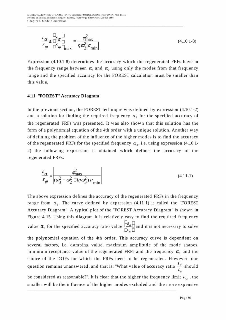
MODEL VALIDATION OF LARGE FINITE ELEMENT MODELS USING TEST DATA, PhD ThesisNedzad Imamovic, Imperial College of Science, Technology & Medicine, London 1998
Chapter 4. Model Correlation__________________________________________________________________________________________
______________________________________________________________________________________
Page 91
εαεφ
≤εαεφ
max
=φmax
2
ηω22 α
min
(4.10.1-8)
Expression (4.10.1-8) determines the accuracy which the regenerated FRFs have inthe frequency range between ω1 and ω2 using only the modes from that frequency
range and the specified accuracy for the FOREST calculation must be smaller thanthis value.
4.11. "FOREST" Accuracy Diagram
In the previous section, the FOREST technique was defined by expression (4.10.1-2)and a solution for finding the required frequency ω3 for the specified accuracy of
the regenerated FRFs was presented. It was also shown that this solution has theform of a polynomial equation of the 4th order with a unique solution. Another wayof defining the problem of the influence of the higher modes is to find the accuracyof the regenerated FRFs for the specified frequency ω3 , i.e. using expression (4.10.1-
2) the following expression is obtained which defines the accuracy of theregenerated FRFs:
εαεφ
=φmax
2
(ω32 − ω2
2 + iηω32 ) α
min
(4.11-1)
The above expression defines the accuracy of the regenerated FRFs in the frequencyrange from ω2 . The curve defined by expression (4.11-1) is called the "FOREST
Accuracy Diagram". A typical plot of the "FOREST Accuracy Diagram" is shown inFigure 4-15. Using this diagram it is relatively easy to find the required frequency
value ω3 for the specified accuracy ratio value εα
εφ
and it is not necessary to solve
the polynomial equation of the 4th order. This accuracy curve is dependent onseveral factors, i.e. damping value, maximum amplitude of the mode shapes,minimum receptance value of the regenerated FRFs and the frequency ω2 and the
choice of the DOFs for which the FRFs need to be regenerated. However, one
question remains unanswered, and that is: "What value of accuracy ratio εα
εφ
should
be considered as reasonable?". It is clear that the higher the frequency limit ω3 , the
smaller will be the influence of the higher modes excluded and the more expensive

MODEL VALIDATION OF LARGE FINITE ELEMENT MODELS USING TEST DATA, PhD ThesisNedzad Imamovic, Imperial College of Science, Technology & Medicine, London 1998
Chapter 4. Model Correlation__________________________________________________________________________________________
______________________________________________________________________________________
Page 92
are the calculations required to extract the necessary modes. Considering the shapeof the accuracy curve (see Figure 4-15) it can be seen that after some frequency valueω3 the accuracy actually changes very little and any calculation of the modes above
that frequency is not necessary. In order to find the optimum value of the frequencyω3 it is recommended that the first derivative of expression (4.11-1) be consideredand then that the frequency ω3 be selected as the first derivative value approacheszero. This would mean that above the selected frequency, ω3 , the change in the
accuracy value is insignificant. The first derivative of the accuracy function isdefined by the following expression:
dεα
ε φ
d ω3( ) = −2 φmax
2 ω3 ω32 − ω2
2( )+ η2ω33[ ]
α min ω32 − ω2
2( )2+ η2ω3
4[ ]3
2
(4.11-2)
A typical plot of the first derivative of the FOREST accuracy function is shown inFigure 4-16.
Figure 4.15. ‘FOREST’ Accuracy Diagram.
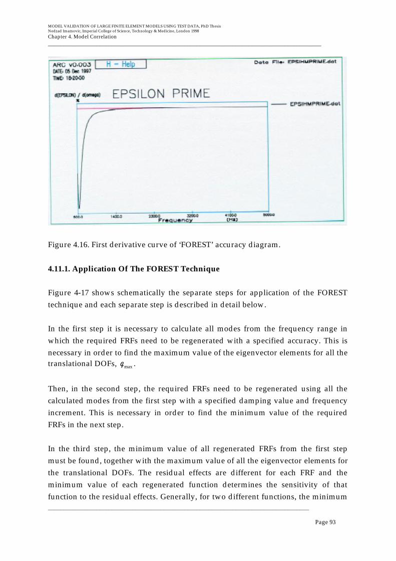
MODEL VALIDATION OF LARGE FINITE ELEMENT MODELS USING TEST DATA, PhD ThesisNedzad Imamovic, Imperial College of Science, Technology & Medicine, London 1998
Chapter 4. Model Correlation__________________________________________________________________________________________
______________________________________________________________________________________
Page 93
Figure 4.16. First derivative curve of ‘FOREST’ accuracy diagram.
4.11.1. Application Of The FOREST Technique
Figure 4-17 shows schematically the separate steps for application of the FORESTtechnique and each separate step is described in detail below.
In the first step it is necessary to calculate all modes from the frequency range inwhich the required FRFs need to be regenerated with a specified accuracy. This isnecessary in order to find the maximum value of the eigenvector elements for all thetranslational DOFs, φmax .
Then, in the second step, the required FRFs need to be regenerated using all thecalculated modes from the first step with a specified damping value and frequencyincrement. This is necessary in order to find the minimum value of the requiredFRFs in the next step.
In the third step, the minimum value of all regenerated FRFs from the first stepmust be found, together with the maximum value of all the eigenvector elements forthe translational DOFs. The residual effects are different for each FRF and theminimum value of each regenerated function determines the sensitivity of thatfunction to the residual effects. Generally, for two different functions, the minimum
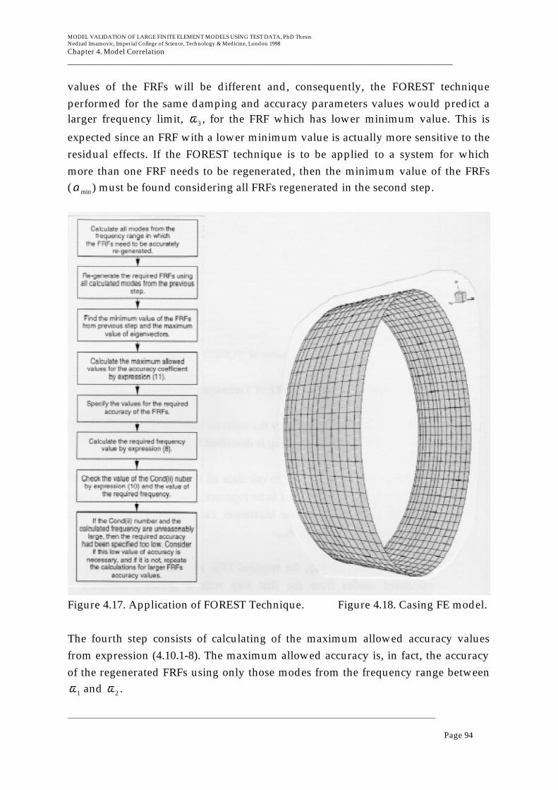
MODEL VALIDATION OF LARGE FINITE ELEMENT MODELS USING TEST DATA, PhD ThesisNedzad Imamovic, Imperial College of Science, Technology & Medicine, London 1998
Chapter 4. Model Correlation__________________________________________________________________________________________
______________________________________________________________________________________
Page 94
values of the FRFs will be different and, consequently, the FOREST techniqueperformed for the same damping and accuracy parameters values would predict alarger frequency limit, ω3 , for the FRF which has lower minimum value. This is
expected since an FRF with a lower minimum value is actually more sensitive to theresidual effects. If the FOREST technique is to be applied to a system for whichmore than one FRF needs to be regenerated, then the minimum value of the FRFs(α min) must be found considering all FRFs regenerated in the second step.
Figure 4.17. Application of FOREST Technique. Figure 4.18. Casing FE model.
The fourth step consists of calculating of the maximum allowed accuracy valuesfrom expression (4.10.1-8). The maximum allowed accuracy is, in fact, the accuracyof the regenerated FRFs using only those modes from the frequency range betweenω1 and ω2 .
MODEL VALIDATION OF LARGE FINITE ELEMENT MODELS USING TEST DATA, PhD ThesisNedzad Imamovic, Imperial College of Science, Technology & Medicine, London 1998
Chapter 4. Model Correlation__________________________________________________________________________________________
______________________________________________________________________________________
Page 95
In the fifth step, the required accuracy for the regenerated FRFs is specified, and thismust be less than the maximum allowed accuracy calculated in the fourth step. Thisis necessary in order to obtain a realistic solution for the required cut-off modefrequency, ω3 . Normally, the accuracy parameters are specified as two differentquantities, εα for the minimum value of the FRFs, αmin , and εφ for the maximum
eigenvector value of the translational DOFs, φmax . Usually, εα is specified as apercentage of the αmin value, i.e. 1 to 5 % is recommended, and εφ is specified as a
multiple of the φmax value.
The required frequency value, ω3 , is calculated from expression (4.10.1-5) in the
sixth step.
The seventh step includes calculation of the Cond (II) number and checking thevalues of Cond (II) and frequency ω3 . If the values of Cond (II) and ω3 are
unreasonably large, due to specifying too small an accuracy value in the fifth step, itshould be considered whether this high accuracy is necessary and, if it is not, thennew calculations should be performed from the fifth step.
4.11.2. Application of the FOREST Accuracy Diagram
After supplying a minimum receptance value, α min , maximum amplitude value,φmax , damping value, η , and the frequency, ω4 , the expressions (4.11-1) and (4.11-2)
can be used to calculate the "FOREST Accuracy Diagram" (see Figure 4-15) and thederivative of the accuracy function (see Figure 4-16) in the frequency rangebetweenω2 and ω4 . This frequency, ω4 , represents the upper limit of interest whichis usually more than 10 times of the ω2 frequency value. In order to select theoptimum frequency value, ω3 , both diagrams should be considered, noting that theoptimum frequency ω3 value is where the derivative curve of the accuracy function
approaches zero, i.e. that means that there is no significant change in the accuracy ofthe regenerated FRFs.
4.12. FOREST Test Case Study
A structure whose model has 9542 DOF (see Figure 4-18) was used as a test casestudy for application of the FOREST technique. It is clear that for this size structurea direct FRF regeneration approach is practically impossible. Figure 4-11 shows thepoint FRFs for point 1 regenerated by the modal approach using 65 and 500 modes.

MODEL VALIDATION OF LARGE FINITE ELEMENT MODELS USING TEST DATA, PhD ThesisNedzad Imamovic, Imperial College of Science, Technology & Medicine, London 1998
Chapter 4. Model Correlation__________________________________________________________________________________________
______________________________________________________________________________________
Page 96
The influence of the residuals on the FRF which was regenerated using 65 modes isvery high, but calculation using 500 modes is quite expensive, so the FORESTtechnique will be applied in order to find an optimal accuracy-dependent requirednumber of modes.
The FOREST technique is applied in the following steps:
1. 65 modes are known to exist in the frequency range between 0 and 500 Hz, inwhich range the point FRF for point 1 needs to be regenerated with a givenaccuracy.
2. The point FRF is regenerated in the frequency range between 0 and 500 Hz usingall 65 modes calculated from the previous step, for the specified damping value ofη = 0.003 and a frequency increment of 1 Hz.
3. The minimum receptance value of the FRF is α min = −140 dB and the maximum
value of the eigenvector elements is φmax = 0.476 kg( )−1
2 .
4. The maximum allowed ratio for the accuracy coefficient is εα
εφ
max
= 0.774 .
5. The specified accuracy parameters are εα = 5 % and εφ = 2 , or εα
εφ
= 2.5 % , well
below the maximum allowed values.
6. The required frequency is ω3 = 1565.7 Hz .
7. The condition number, Cond (II) is equal to 30.9, and this is considered to bereasonable as well as the value of the required frequency, ω3 = 1565.7 Hz , which is
about three times the value of the upper limit frequency ω2 = 500 Hz .
Now, calculating all modes in the frequency range between 0 and ω3 = 1565.7 Hz it
is found that there are 378 modes which must be included for the FRF regenerationto attain the specified accuracy. Figure 4-19 shows the same FRF but regeneratedusing 65, 378 and 500 modes. It is clear that little improvement is obtained if modesafter the FOREST predicted frequency, ω3 are included.

MODEL VALIDATION OF LARGE FINITE ELEMENT MODELS USING TEST DATA, PhD ThesisNedzad Imamovic, Imperial College of Science, Technology & Medicine, London 1998
Chapter 4. Model Correlation__________________________________________________________________________________________
______________________________________________________________________________________
Page 97
The "FOREST Accuracy Diagram" was generated in the frequency range between500 and 5000 Hz. The FOREST accuracy function for this case is shown in Figure 4-15 and the derivative of the FOREST accuracy function is shown in Figure 4-16. Byconsidering these curves it is relatively easy to conclude that the optimumfrequency value ω3 is around 1500 Hz.
Figure 4.19. FRFs regenerated using 65, 378 and 500 modes.
4.13. Co-ordinate Modal Assurance Criterion (COMAC)
Co-ordinate Modal Assurance Criterion (COMAC) has been in use for a number ofyears, first introduced by Lieven 1988 [11]. COMAC is mathematically derived fromthe MAC, the only difference is that MAC is the scalar product between two modeshapes for all DOFs, whilst the COMAC is the scalar product between two vectorsthat represent two DOFs for a number of selected corresponding mode shapes. Thisdefinition implies that the knowledge of the CMPs is necessary for calculation ofthis correlation coefficient and therefore this correlation procedure is moresignificant as a refined correlation tool for assessment of global correlation. Its major

MODEL VALIDATION OF LARGE FINITE ELEMENT MODELS USING TEST DATA, PhD ThesisNedzad Imamovic, Imperial College of Science, Technology & Medicine, London 1998
Chapter 4. Model Correlation__________________________________________________________________________________________
______________________________________________________________________________________
Page 98
advantage is that it shows the correlation between two DOFs for number of modes,and if it is found that there is little agreement for some DOF pairs, then they shouldbe checked and possibly removed from data sets if appropriate.
Mathematically, the COMAC correlation coefficient is defined in the followingexpression:
COMAC(DoFi, DoFj) =φ i ,rφ j ,r
*
r = 1
m
∑
2
( φ i,r φi ,r*
r = 1
m
∑ )( φ j ,rφ j ,r*
r= 1
m
∑ )(4.13-1)
where index r represents the correlated mode pairs from each set of data.Application of this method is demonstrated in Figure 4-20 using SAMM II Bstructure test case.
A useful application of this correlation coefficient will be described in weighting ofupdating equation later in the text.
Figure 4.20. A typical COMAC results.

MODEL VALIDATION OF LARGE FINITE ELEMENT MODELS USING TEST DATA, PhD ThesisNedzad Imamovic, Imperial College of Science, Technology & Medicine, London 1998
Chapter 4. Model Correlation__________________________________________________________________________________________
______________________________________________________________________________________
Page 99
4.14. Conclusion
A new correlation procedure which can be used during model updating as anautomatic tool for mode pairing is presented in this paper. The method combinesthe minimum data requirements necessary for successful application of a correlationcoefficient based on SEREP reduction of the theoretical model. The advantages ofthe SEREP-based correlation coefficients over MAC or NCO are demonstrated. TheSEREP Cross Orthogonality (SCO) correlation technique is more sensitive than MACor NCO techniques, i.e., it will show similarities with higher values than MAC orNCO for similar modes, and vice-versa it will have lower values for independentmodes.
Also, a method for assessment of the modal complexity of experimental modes hasbeen presented which helps to assess global quality of experimental data. Inaddition, a useful realisation process has been described that can be used prior tocorrelation and updating.
The FOREST technique is a simple method for determining the required number ofmodes for the modal summation approach to FRF regeneration with a specifiedaccuracy or for determining the accuracy which will be obtained with a specifiednumber of modes. The method is simple to use and does not require anycomplicated calculations. The method was originally developed to be used formodel correlation purposes in FRF-based updating methods and, since therotational DOFs cannot be easily measured experimentally the method considersonly translational DOF.
MODEL VALIDATION OF LARGE FINITE ELEMENT MODELS USING TEST DATA, PhD ThesisNedzad Imamovic, Imperial College of Science, Technology & Medicine, London 1998
Chapter 5. Error Location Theory__________________________________________________________________________________________
______________________________________________________________________________________
Page 100
5.0 Error Location Theory
5.1. Introduction
Error location is probably the most difficult part of the model validation. Errorlocation can be defined as the process of finding and isolating the parts in the modelof the structure which it is believed are responsible for the observed discrepanciesbetween the theoretical predictions and the measurements. Unfortunately, there isno simple direct procedure which can localise the error in the structural model onthe basis of experimental data. Instead, most existing updating procedures localiseerrors in the model and update the model simultaneously. In order to localise theerror in the model properly, all possible model definition parameters should beselected as updating parameters, and this means that for a system with N degrees-of-freedom, the maximum number of updating parameters is N N +1( ) , assuming
completely dense system matrices, and excluding damping in order to simplify theproblem. This would further mean that the measured data requirement should haveat least the same amount of information as the number of updating parameters, i.e.all natural frequencies and mode shapes should be measured at all co-ordinates, inorder to be able to solve the updating and error location equation uniquely.
In practice, it is not possible to overcome the experimental data incompletenessproblem: it is theoretically possible to measure frequency responses up to 100 kHz,but practically this value drops to about 5-20 kHz due to the limitations given insection 3.2. Also, the number of measurement positions is limited by access and timeconstraints, and it can never match the number of theoretical DOFs. Since numericalmethods are approximate methods - see Chapter 2 - only a limited number of modesfrom equations 2.4-4 and 2.4-5 will converge to numerically-accurate solutions ofthese equations (this does not mean that the converged accurate solutions are ingood agreement with experimental modes).
This discussion leads to the inevitable conclusion that there are some constraints(lack of experimental data and imperfection of theoretical models) which make theerror location almost impossible to solve exactly using any deterministic approach.Even if these limitations are somehow resolved, error location using experimentaldata cannot be guaranteed because a particular theoretical model may be of such aconfiguration that it can never represent the experimental behaviour accurately.

MODEL VALIDATION OF LARGE FINITE ELEMENT MODELS USING TEST DATA, PhD ThesisNedzad Imamovic, Imperial College of Science, Technology & Medicine, London 1998
Chapter 5. Error Location Theory__________________________________________________________________________________________
______________________________________________________________________________________
Page 101
This does not mean that the error location problem cannot be tackled - in fact thereare several approaches for selecting updating parameters - and these methods arediscussed in more detail in this chapter.
5.1.1. Identification Approach
It has been said in previous sections that measured data are incomplete in respect ofthe number of measured modes as well as in respect of the number of measurementpoints. However, if it was possible to measure all natural frequencies and all modes,then it would be possible to perform a simple identification of the spatial propertiesof the system (the global mass and stiffness matrices) from the modal properties (thenatural frequencies and mode shapes) using the orthogonality equations (2.4-6) and(2.4-7) [38][39][40][22]. Unfortunately, the measurement frequency range is limited,as defined by equation (3.2-4), and usually the maximum practical measuredfrequency limit is below 50 kHz in practice. By solving a special eigenvalue problemfor a symmetric system matrix A[ ] it is possible to obtain the following expression
[29]:
A[ ]= ψ{ }rλ r ψ{ }
r
T
r =1
N
∑ (5.1.1-1)
where vectors ψ{ }r are found by solving the special eigenvalue problem:
( A[ ]− λ r I[ ]) ψ{ }r
= 0{ } (5.1.1-2)
and vectors ψ{ }r are normalised according the following expression:
ψ[ ]T ψ[ ]= I[ ] (5.1.1-3)
By analysing the right hand side of expression (5.1.1-1), it can be concluded thatsince all eigenvector elements, ψ r, j , have the same order of magnitude values, and
the eigenvalue λ r is consistently rising as the mode number increases, the values of
the system matrix terms are numerically dominated by the higher frequency modes.This means that from the identification point of view, eigenvector with loweigenvalues are not of much use since they do not contribute any significant amountto the system matrix element values. Unfortunately, due to reasons given earlier

MODEL VALIDATION OF LARGE FINITE ELEMENT MODELS USING TEST DATA, PhD ThesisNedzad Imamovic, Imperial College of Science, Technology & Medicine, London 1998
Chapter 5. Error Location Theory__________________________________________________________________________________________
______________________________________________________________________________________
Page 102
using expression (3.2-4), it is not possible to measure the higher frequency modes:even if it was possible to measure the FRFs in the high frequency range, themeasured FRFs become very unfriendly for modal parameter identification sincedamping becomes more influential for the higher modes.
One might think that, after measuring a certain (practically reasonable) number ofmodes (e.g. 10) at the same number of locations (i.e. 10), and after performingmodal analysis of the measured FRFs, the identification approach (expressions (2.4-6) and (2.4-7)) would certainly lead to mass and stiffness system matrices of size10x10 which would be of full rank. However, these matrices cannot be used forfurther analysis (static, general dynamic etc.) since the actual value of each of thestiffness matrix element would be just a fraction of the real stiffness value which ismainly dominated by the higher frequency modes, although the eigensolutionwould not change from the values which were initially used to construct thesematrices.
5.2. Causes of Discrepancies in Model Validation
5.2.1. Introduction
Most discrepancies in real correlation test cases are blamed on some unspecifiederrors in the finite element model. Experience also shows that there is a tendency fortheoretical analysts to explain discrepancies through inaccurate measurement data,whilst the experimentalists would hold the theoretical model responsible for thediscrepancies. Although the experimental data are used to validate the finiteelement models - not vice versa - this does not mean that all discrepancies are due toimperfect finite element models. The experimental data are of limited accuracy andit is absolutely crucial to check whether measured data are repeatable and also anyother non-linearities must be detected if they exist. Usually, most engineeringstructures are designed so that they should retain more or less the same dynamiccharacteristics throughout their working life. Moreover, it is expected that twostructures coming from the same production series would be identical andconsequently would have identical dynamic properties. Unfortunately, this is notthe case in practice and it is not unusual to come across examples that demonstratesignificant difference in dynamic properties for two structures thought to beidentical. Clearly, it can be concluded that both the experimental data andtheoretical modelling share responsibilities for discrepancies observed in

MODEL VALIDATION OF LARGE FINITE ELEMENT MODELS USING TEST DATA, PhD ThesisNedzad Imamovic, Imperial College of Science, Technology & Medicine, London 1998
Chapter 5. Error Location Theory__________________________________________________________________________________________
______________________________________________________________________________________
Page 103
correlation, although the degree of responsibilities are generally different as isexplained in the following sections [41].
In order to ilustrate the above discussion, an example is selected to demonstratepotential difficulties when trying to explain descrepancies between test andpredicted data. An assembled stucture is shown in Figure 5.2.1-1. The structure isassembled from several pieces and it is bolted to a large steel block in order tosimulate clamped boundary conditions. Comparison between measured andpredicted FRFs is shown in Figure 5.2.1-2. Clearly, the two models are quitedifferent and initially the majority of descrepancies were thought to be caused byinappropriate modelling of structural joints. However, later on it was shown thatthe individual components had certain descrepancies even though they all are one-piece components.
MODEL VALIDATION OF LARGE FINITE ELEMENT MODELS USING TEST DATA, PhD ThesisNedzad Imamovic, Imperial College of Science, Technology & Medicine, London 1998
Chapter 5. Error Location Theory__________________________________________________________________________________________
______________________________________________________________________________________
Page 104
5.2.2. Errors in Experimental Data
Generally, the accuracy of the measured natural frequencies is higher then theaccuracy of the mode shapes. The accuracy of measured FRFs varies for differentfrequency values, [2] - it is higher around resonances and lower around anti-resonances due to different signal-to-noise ratios - and also the accuracy depends onmeasurement position for the same reason. If, for instance, a measurement positionis located near the nodal line of a mode, then the response signal around naturalfrequency of that mode will have a low value and inevitably the relative accuracy ofthe measured FRF will be smaller than relative accuracy of FRFs for points whichare located away from the nodal lines of that mode. However, it should be stressedhere that this loss of relative accuracy is not so serious since the absolute value ofthe response at the measured position located near the nodal line will have a smallvalue. The planning of modal tests in Chapter 3 deals with the problem of selectionof best measurement locations in order to improve the accuracy of measured data.
5.2.3. Errors in Finite Element Modelling
It is not possible to prescribe any values for the accuracy of the theoreticalpredictions. The term ‘accuracy of theoretical predictions’ has a twofold meaninghere. The first one is the converged accuracy of the model, i.e. the accuracy of thedynamic properties in respect to the mesh density used on the model. Because thiserror is so common in practice it will be given the name the mesh distortion related
error [31]. The second meaning is the accuracy with respect to the experimentalvalues observed in the correlation. In most practical situations it is observed that inorder to improve correlation significantly it is necessary to change the configurationof the model and therefore this type of error is called the configuration related
error.
For instance, if a measured frequency value is 15.1 Hz and the correspondingpredicted value is 25.5 Hz, the first suspect for this discrepancy is the theoreticalmodel because the discrepancy is so high that if there is any doubt in the accuracyof the experimental data on this scale then the whole experimental data set isunreliable for validating the theoretical model. If, however, the density of the meshis increased several times to a number of DOFs where there is no change to thevalue of the natural frequency which is now 23.3 Hz, then this means that there is

MODEL VALIDATION OF LARGE FINITE ELEMENT MODELS USING TEST DATA, PhD ThesisNedzad Imamovic, Imperial College of Science, Technology & Medicine, London 1998
Chapter 5. Error Location Theory__________________________________________________________________________________________
______________________________________________________________________________________
Page 105
something more fundamentally wrong with the model, i.e. the configuration of themodel is the next suspect for the correlation discrepancies.
Mesh Distortion Related Errors
In order to generate either mass or stiffness matrices for a finite element it isnecessary to perform integration over the domain of that element as indicated inexpressions (2.3.1-3) and (2.3.1-4). The global and local co-ordinate systems arerelated non-linearly via the Jacobian matrix and in the case of an extremelydistorted element, the Jacobian matrix can become singular and therefore this caninfluence the values of structural matrix. This problem can be overcome by dividingdistorted elements into several less distorted elements and an example of theinfluence of the mesh on the eigenvalue solution is given below [42]. The structuralcomponent shown in Figure 5.2.3-1 is modelled using two different meshes. Model‘A’ has 20,000 DOFs, whilst the second model ‘B’ shown in Figure 5.2.3-2 has 45,000DOFs. Figures 5.2.3-3 and -4 shows the two theoretical FRFs re-generated frommodels ‘A’ and ‘B’ on the same plot with the corresponding experimental FRF. Thisexample clearly demonstrates vulnerability of finite element modelling to this typeof error.
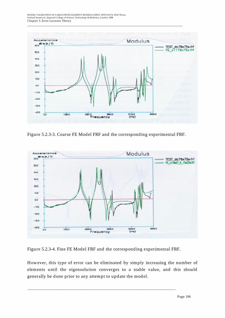
MODEL VALIDATION OF LARGE FINITE ELEMENT MODELS USING TEST DATA, PhD ThesisNedzad Imamovic, Imperial College of Science, Technology & Medicine, London 1998
Chapter 5. Error Location Theory__________________________________________________________________________________________
______________________________________________________________________________________
Page 106
Figure 5.2.3-3. Coarse FE Model FRF and the corresponding experimental FRF.
Figure 5.2.3-4. Fine FE Model FRF and the corresponding experimental FRF.
However, this type of error can be eliminated by simply increasing the number ofelements until the eigensolution converges to a stable value, and this shouldgenerally be done prior to any attempt to update the model.

MODEL VALIDATION OF LARGE FINITE ELEMENT MODELS USING TEST DATA, PhD ThesisNedzad Imamovic, Imperial College of Science, Technology & Medicine, London 1998
Chapter 5. Error Location Theory__________________________________________________________________________________________
______________________________________________________________________________________
Page 107
Configuration Related Errors
Errors of this type are the most common ones found to be responsible fordiscrepancies observed in practice. When any uncertainty that could exist betweenthe model and the real structure is resolved, i.e. material properties, geometricalrepresentation of the structure, physical properties of some elements etc., and if thediscrepancies are still larger than the uncertainty of the accuracy of the experimentaldata, then the model is likely to be of the wrong configuration. The term ‘wrongconfiguration’ is a very broad term and could mean any of several differentimperfections that model possesses. If, for instance, a simple plate is modelled, thenit is very unlikely to expect that the model could be of wrong configuration, but ifthere is a crack inside the structure that is not included in the model, then even suchsimple model could be of wrong configuration.
Another inevitable example of wrong configuration is modelling of structural joints.Structural joints are regions where two components of a structure are permanentlyconnected. There are several reasons why structural joints are difficult to model. It isalmost impossible to find a precise description of structural joints. Practicalinspection of structures will disclose that there is often an unspecified inconsistencybetween the description of structural joints in technical drawings and in reality. It isextremely difficult to determine contact areas between the two parts that areconnected by a structural joint. Moreover, it is possible that the contact area is notconsistent during vibration. This type of structural joint will almost inevitablyintroduce some non-linear effects in the dynamic behaviour of structures.
Modelling of structural joints is critical for the accuracy of the theoreticalpredictions. There are two approaches for modelling structural joints: (i) oneemployes a simplification of the joints and (ii) the other one involves detailedmodelling of the joints. Oversimplification of structural joints is almost certain tolead to an inadequate representation of real connections and consequently this willaffect the accuracy of the predicted dynamic characteristics. In contrast to thesimplification approach, a particularly detailed modelling of structural joints isunlikely to improve the accuracy of the theoretical predictions because the verydetails of structural joints are unknown and consequently these inaccuracies aretransferred to the model. The recommended approach for modelling of structuraljoints is to have a proper balance between these two approaches: neither anextremely simplified nor an extremely detailed model.
MODEL VALIDATION OF LARGE FINITE ELEMENT MODELS USING TEST DATA, PhD ThesisNedzad Imamovic, Imperial College of Science, Technology & Medicine, London 1998
Chapter 5. Error Location Theory__________________________________________________________________________________________
______________________________________________________________________________________
Page 108
5.3. Updating Parameters Definition
There is no restriction to what could be an updating parameter and anything thatmakes changes to the theoretical model predictions can be selected, as the followingexpression indicates:
λ r , φ{ }r
= function p1, .. ., pl( ), r = 1,.., N (5.3-1)
All updating parameters can be divided into two groups; one is for the wholematrix correction and the other group is selective updating parameters. There aretwo different types of selective updating parameter, one is the spatial-type andanother is the design-type. Also, there is a particular general spring-like updatingparameter which is the most basic updating parameter.
5.3.1. Whole Matrix Updating Parameters
A whole-matrix updating parameter can be defined as the a simple correction to theentire system matrices, as indicated in the following expressions:
KU[ ]= KA[ ]+ ∆KU[ ] (5.3.1-1)
MU[ ]= MA[ ]+ ∆MU[ ] (5.3.1-2)
The main disadvantage of this type of updating parameter is that there is no controlover which particular elements are selected for updating. Also, after updating, theoriginal connectivity of the model could be lost. Since the whole matrix correctionwould destroy the initial connectivity of the global mass or stiffness matrices, thisprocedure has a particular disadvantage in the application for updating of largefinite element models because it will make the system matrices dense andconsequently difficult or practically impossible to handle.

MODEL VALIDATION OF LARGE FINITE ELEMENT MODELS USING TEST DATA, PhD ThesisNedzad Imamovic, Imperial College of Science, Technology & Medicine, London 1998
Chapter 5. Error Location Theory__________________________________________________________________________________________
______________________________________________________________________________________
Page 109
5.3.2. Spatial-type Updating Parameters
The spatial-type parameters are defined as the products of an updating coefficientand a macro element matrix which has the same format as its correspondingassembled spatial system matrix (mass, stiffness or damping). This is, in effect, alinearisation of the updating equation through an assumption of linear distributionof errors in the model. The changes to the initial matrices are defined as follows, forthe global mass matrix, for example:
∆MU[ ]= pr Mre[ ]
r =1
pM
∑ (5.3)
and for the global stiffness matrix as,
∆KU[ ]= pr Kre[ ]
r =1
pK
∑ (5.4)
where Mre[ ] and Kr
e[ ] are macro-element matrices for mass and stiffness updating
parameters, respectively. Macro elements, Mre[ ] or Kr
e[ ], can possess the same
connectivity as the initial model, i.e. no extra elements would be introduced, or iftheir connectivity is generally different from that of the initial matrices then extraelements would be created and the initial connectivity would be destroyed. Theupdated mass and stiffness matrices would then be defined by the followingequations:
MU[ ]= MA[ ]+ p1 ∆M1e[ ]+ ... +ppM
∆MpM
e[ ] (5.5)
KU[ ]= KA[ ]+ p1 ∆K1e[ ]+ .. .+ ppK
∆KpK
e[ ] (5.6)
An advantage of this type of updating parameter definition is that it is very general,but a disadvantage is that there is limited physically-meaningful explanation forthis kind of change of the structural model.

MODEL VALIDATION OF LARGE FINITE ELEMENT MODELS USING TEST DATA, PhD ThesisNedzad Imamovic, Imperial College of Science, Technology & Medicine, London 1998
Chapter 5. Error Location Theory__________________________________________________________________________________________
______________________________________________________________________________________
Page 110
5.3.3. Design-type Updating Parameters
The third updating parameter type is the design-type, and is defined as any designinput parameter of the initial model. There is no restriction on what the updatingparameter could be as long as it provides the desired changes to the eigensolution ofthe system. Examples of this updating parameter are: material properties of eachfinite element, geometrical properties of finite elements, thickness of the shellelements, beam element diameter, area, moments of inertia, torsion constant, etc..The main disadvantage of this type of updating parameter is that there is a limitednumber of them and they may not provide enough variables to update a structuresuccessfully since they cannot change the configuration of a model. However, anadvantage of this type of updating parameter is that they represent physicalchanges in the structure, which are physically meaningful.
5.3.4. General Spring-like Updating Parameters
The general spring-like updating parameter is a simple spring element that connectstwo degrees-of-freedom. If the whole-matrix correction is one extreme type ofupdating parameter that does not allow any selection of finite elements, the generalspring-like element is the most basic updating parameter that represents theconnection between two individual DOFs. Model updating is basically the processof changing the values in the global stiffness or mass matrices, but there are someminimum requirements that have to be fulfilled when modifying these matrices.The global mass and stiffness matrices are symmetric and therefore any updatingchanges have to be symmetric in order to keep the updated system matricessymmetric. Another important condition is the reciprocity between two DOFs. Thismeans that if there are two DOFs that belong to a updating parameter, then anychange to the stiffness or mass values in the global matrices have to be of the samevalues for both DOFs.

MODEL VALIDATION OF LARGE FINITE ELEMENT MODELS USING TEST DATA, PhD ThesisNedzad Imamovic, Imperial College of Science, Technology & Medicine, London 1998
Chapter 5. Error Location Theory__________________________________________________________________________________________
______________________________________________________________________________________
Page 111
The change of the global mass or stiffness matrix can be represented symbolically inthe following expression:
k1,1
− k1,1U k
1, 2k
1,3+ k
1, 3U k
1,4
k2,1
k2,2 k2,3 k2, 4
k3,1
+ k3,1U k3,2 k3,3 − k3,3
U k3, 4
k4,1
k4,2 k4,3 k4, 4
=
k1,1 k1,2 k1, 3 k1,4
k2, 1 k2, 2 k2,3 k2, 4
k3, 1 k3, 2 k3,3 k3, 4
k4, 1 k4, 2 k4,3 k4, 4
+−k
1,1U k
1, 3U
k3,1U −k3, 3
U
(5.3.4-1)
In fact, the matrix −k
1,1U k
1, 3U
k3,1U −k3, 3
U
represents the most basic change to the global
stiffness matrix, and also there are additional conditions as shown in the followingexpression:
k1,1U = k3,3
U (5.3.4-2)
k1,3U = k3,1
U (5.3.4-3)
The reciprocity condition is described in expression (5.3.4-2) whilst expression(5.3.4-3) describes the symmetry condition. Also, the global matrices have to bediagonally dominant, and that is described in the following expression:
k1, 1U ≥ k3,1
U (5.3.4-4)
A simple spring element is defined by k1,1U = k3,1
U which is the simplest physically
meaningful updating parameter.
The bandwidth of a sparse matrix is defined as the largest number of coupled DOFsfor any column or row in the matrix. This coupling of DOFs is determined by thetype of finite elements used in the model, i.e. a simple spring couples two DOFs,whilst the higher the order of the finite element formulation the larger the numberof coupled DOFs. Generally, it can be assumed that all DOFs connected by one finiteelement are fully coupled amongst themselves, whilst the bandwidth of the matrixwill depend on inter-elemental connections in the model.
By introducing the spring-like element it becomes possible to change theconfiguration of the model, i.e. it is possible to couple two DOFs that belong to one

MODEL VALIDATION OF LARGE FINITE ELEMENT MODELS USING TEST DATA, PhD ThesisNedzad Imamovic, Imperial College of Science, Technology & Medicine, London 1998
Chapter 5. Error Location Theory__________________________________________________________________________________________
______________________________________________________________________________________
Page 112
finite element additionally if the original finite element is not capable ofrepresenting the experimental results accurately.
5.3.5. Limitations of Updating Parameters Value
Apart from the above-mentioned properties of the finite element, i.e. symmetry,reciprocity and diagonal dominance, there are some other requirement that have tobe fulfilled if the model is considered to be properly defined. The stiffness matrixmust not be numerically singular or near-singular or ill-conditioned. Theserequirements are used to derive the limitations for the updating parameter valuesduring model updating process.
It is important to stress here that there are two possible causes for singularity ofstiffness matrix. One reason for such singularity could be due to boundaryconditions which enable the structure to move freely in one or more generaliseddirections. In this case, we expect to find the same number of rigid-body-modes(RBMs) as the number of unconstrained generalised directions for the wholestructure. Another reason for singularity of the stiffness matrix could be due toinadequate representation of some parts of structure or simply due to crudeformulation of stiffness matrix for some elements, or any other reason. Thesingularity of the stiffness matrix described here is assumed not to be caused byexistence of RBMs in model.
Singularity of the stiffness matrix
Any DOF is considered to be singular if [29]
ki, j
kmax
≤ εsing (5.3.5-1)
where ki , j is the term in the i-th row and j-th column and kmax is the largest term inK[ ]. The minimum permitted value for the constant εsing is defined below
εsing = 10−8 (5.3.5-2)
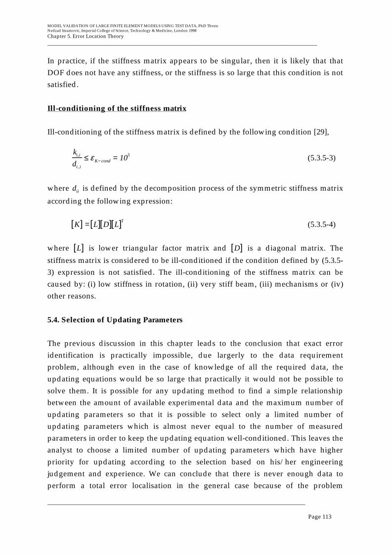
MODEL VALIDATION OF LARGE FINITE ELEMENT MODELS USING TEST DATA, PhD ThesisNedzad Imamovic, Imperial College of Science, Technology & Medicine, London 1998
Chapter 5. Error Location Theory__________________________________________________________________________________________
______________________________________________________________________________________
Page 113
In practice, if the stiffness matrix appears to be singular, then it is likely that thatDOF does not have any stiffness, or the stiffness is so large that this condition is notsatisfied.
Ill-conditioning of the stiffness matrix
Ill-conditioning of the stiffness matrix is defined by the following condition [29],
ki,i
di ,i
≤ ε K− cond = 105 (5.3.5-3)
where dii is defined by the decomposition process of the symmetric stiffness matrix
according the following expression:
K[ ] = L[ ] D[ ] L[ ]T (5.3.5-4)
where L[ ] is lower triangular factor matrix and D[ ] is a diagonal matrix. The
stiffness matrix is considered to be ill-conditioned if the condition defined by (5.3.5-3) expression is not satisfied. The ill-conditioning of the stiffness matrix can becaused by: (i) low stiffness in rotation, (ii) very stiff beam, (iii) mechanisms or (iv)other reasons.
5.4. Selection of Updating Parameters
The previous discussion in this chapter leads to the conclusion that exact erroridentification is practically impossible, due largerly to the data requirementproblem, although even in the case of knowledge of all the required data, theupdating equations would be so large that practically it would not be possible tosolve them. It is possible for any updating method to find a simple relationshipbetween the amount of available experimental data and the maximum number ofupdating parameters so that it is possible to select only a limited number ofupdating parameters which is almost never equal to the number of measuredparameters in order to keep the updating equation well-conditioned. This leaves theanalyst to choose a limited number of updating parameters which have higherpriority for updating according to the selection based on his/her engineeringjudgement and experience. We can conclude that there is never enough data toperform a total error localisation in the general case because of the problem

MODEL VALIDATION OF LARGE FINITE ELEMENT MODELS USING TEST DATA, PhD ThesisNedzad Imamovic, Imperial College of Science, Technology & Medicine, London 1998
Chapter 5. Error Location Theory__________________________________________________________________________________________
______________________________________________________________________________________
Page 114
encountered in measuring the higher frequency modes [40][43]. Instead, a limitednumber of updating parameters is selected by the analyst in those parts of thestructure which are believed to be most uncertain in order to improve correlationwith the experimental data rather then to locate all modelling errors. This alsoleaves a certain amount of possibility for the updating process to fail to improvecorrelation due to reasons of inappropriate selection of updating parameters andthis also makes the updating process case-dependent and the final solution to benon-unique [44][45].
5.4.1. Classification of Methods for Initial Selection of Updating Parameters
Initial selection of updating parameters can be divided in to two basic approachesand these are: (i) an empirical approach and (ii) a sensitivity-based approach. Bothapproaches are manual, i.e. selection is carried out manually by the analyst.
Empirically-based initial selection of updating parameters
This type of initial selection of updating parameters is based on a knowledge of thefinite element model of the structure and approximations built into the initialmodel. In most practical cases, the analyst will compare technical drawings of astructure with the structure itself, and after thorough inspection of the structure aninitial finite element model will be generated. Using this process the analyst canselect several regions of the structure that are not approximated (i.e. modelled) asaccurately as the reminder of the model. These regions of the structure are thenselected in a few updating parameters according to the level of approximation in theinitial model. It is important to notice here that no other knowledge than the level ofapproximation of the initial model is used for this type of selection of updatingparameters.
Sensitivity-based initial selection of updating parameters
This type of initial selection of updating parameters is based on knowledge of thedynamic behaviour of the initial finite element model. When the dynamic propertiesof the initial model are calculated, it is possible to determine the regions of theinitial model that are taking most of strain deformation for a number of modeshapes. The dynamic properties under consideration (i.e. natural frequencies andmode shapes) are clearly highly sensitive to any changes of the model in these high
MODEL VALIDATION OF LARGE FINITE ELEMENT MODELS USING TEST DATA, PhD ThesisNedzad Imamovic, Imperial College of Science, Technology & Medicine, London 1998
Chapter 5. Error Location Theory__________________________________________________________________________________________
______________________________________________________________________________________
Page 115
strain energy regions and therefore these regions are selected as updatingparameters.
5.4.2. Important Factors in Selection of Updating Parameters
A critical stage of the model updating process is the actual selection of updatingparameters, and a real question that the analyst faces is which regions of initialmodel to select as updating parameters. The two approaches described above arevery different and in different situations different approaches should be used. It isnot possible to draw a line between empirical and sensitivity-based updatingparameter selection approaches; instead it is important to understand how theyrelate to and influence the whole course of the model updating process.
The empirical updating parameter selection approach is a fundamentally correctand appropriate method to detect the genuine errors in an initial model. A majoradvantage of this approach is that it is based on an empirical knowledge of theinitial model and the structure itself. The method is expected to select the regions ofstructure which have the largest errors providing that sufficient knowledge aboutthe initial model and structure is available. Unfortunately, this condition may not beeasy to meet in real practical situations, i.e. sometimes it is not possible to inspect astructure, or even if the structure is available it may be impossible to inspect everydetail or some regions of structure may be extremely difficult to assess. Also, aninitial finite element model of a structure may be very complicated, assembled fromseveral sources that were generated by different people or the initial model may bebased on technical drawings that may not be exactly identical to built structure. Thisprocess of assessment of both structure and initial model is extremely dependent onhuman factors (the analyst’s experience) and it can not be easily quantified.
The sensitivity-based updating parameters selection approach selects the regions ofa structure that are most strained for a number of modes under consideration. Usingthis method for selection, the most sensitive parts of the structure are expected to beselected rather than the regions where errors are expected to be found. A majoradvantage of this method is that it is straightforward to use automatically and theuser input in the selection process is limited.
It is difficult to advise which method of selection of updating parameters is moresuitable in the general case. If, for instance, only the empirical selection approach is

MODEL VALIDATION OF LARGE FINITE ELEMENT MODELS USING TEST DATA, PhD ThesisNedzad Imamovic, Imperial College of Science, Technology & Medicine, London 1998
Chapter 5. Error Location Theory__________________________________________________________________________________________
______________________________________________________________________________________
Page 116
used but the dynamic properties under consideration are not sensitive to theselected updating parameters, there is little chance of a successful final result. If,however, only the sensitivity-based selection approach is used, then there is apossibility that accurately modelled regions of a structure are selected as updatingparameters and this will reduce the confidence in the final updated model. Aproper balance of the two methods is recommended, i.e. select both setsindependently and overlay them in order to select updating parameters.
5.5. Objective Function Diagrams
Most updating techniques are, in effect, procedures of optimisation of a definedobjective function, which is usually a global correlation function between thedynamic properties of the analytical and the experimental models. It was alreadynoted that there might not exist a theoretical model, based on a particularformulation (e.g. Finite Element Method), which can represent behaviour of thestructure exactly. Instead, the analyst will try to find a model which is the closest todescribe the behaviour of the structure. Updating procedures are capable of refiningthe structural model in order to bring the discrepancies between the predictions andthe experiment to a minimum possible level.
Errors in the structural model are distributed throughout the model. No matter howsimple a structure’s geometry is and how structural model is refined, the theoreticalmodel of the structure has a finite accuracy in a finite frequency range.
If we consider the simple beam structure shown in Figure 5.5.1. and itscorresponding finite element model shown in Figure 5.5.2., it is generally thoughtthat the finite element model should be able to predict the dynamic behaviour of thestructure very accurately. The correlation between measured and predicted FRFs isshown in Figure 5.5.3. and it can be seen that the discrepancies between the twomodels increase for higher frequencies. One would expect that prediction of such asimple structure with such a fine model should be more accurate than is indicatedin Figure 5.5.3. A natural question after analysing the correlation is: "What are theparameters in the model that are responsible for these discrepancies and how todetect them?". This particular model consists of solid elements and the mesh can beconsidered to be very fine so that any further refinement of the mesh would not belikely to improve correlation significantly. Also, there are no other likely design
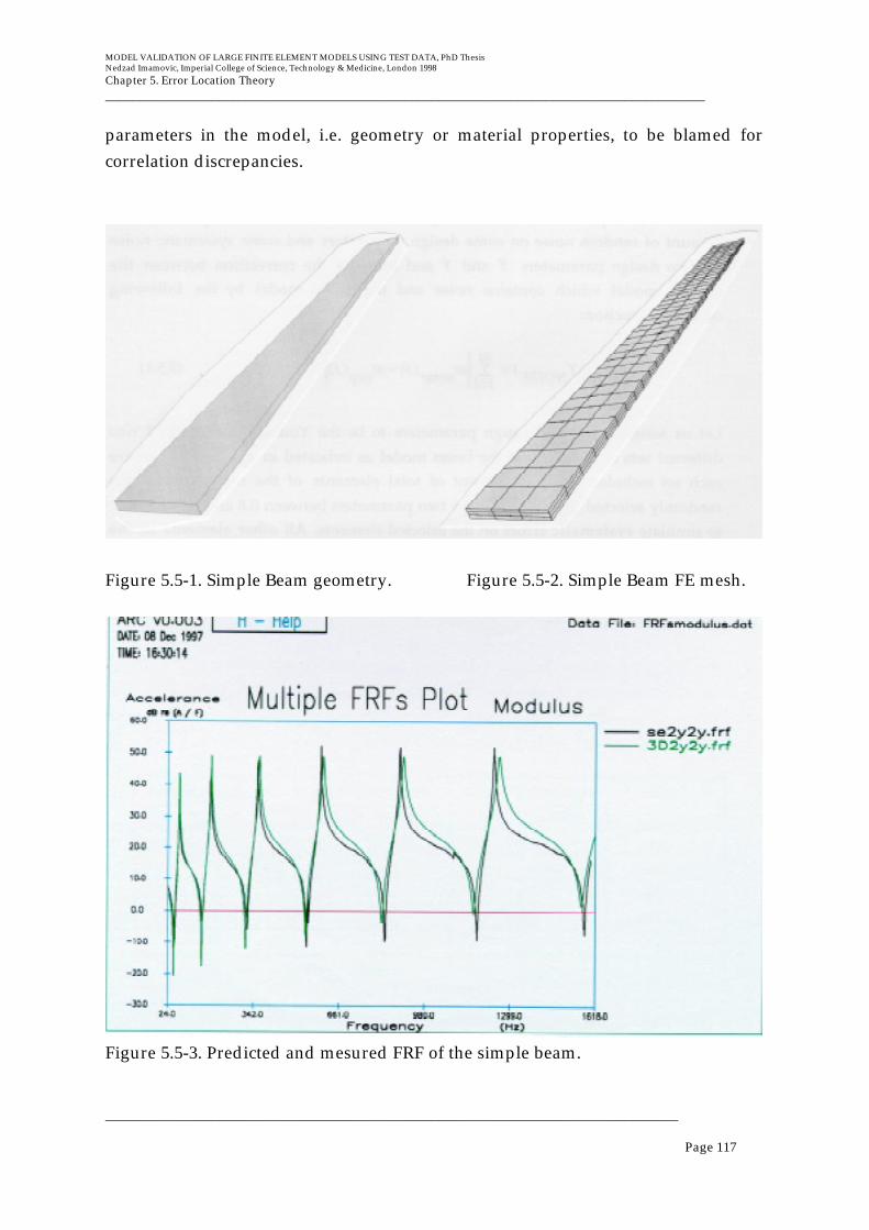
MODEL VALIDATION OF LARGE FINITE ELEMENT MODELS USING TEST DATA, PhD ThesisNedzad Imamovic, Imperial College of Science, Technology & Medicine, London 1998
Chapter 5. Error Location Theory__________________________________________________________________________________________
______________________________________________________________________________________
Page 117
parameters in the model, i.e. geometry or material properties, to be blamed forcorrelation discrepancies.
Figure 5.5-1. Simple Beam geometry. Figure 5.5-2. Simple Beam FE mesh.
Figure 5.5-3. Predicted and mesured FRF of the simple beam.
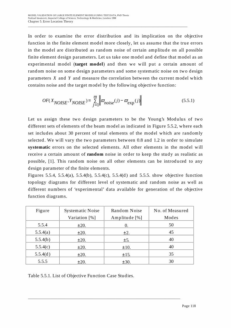
MODEL VALIDATION OF LARGE FINITE ELEMENT MODELS USING TEST DATA, PhD ThesisNedzad Imamovic, Imperial College of Science, Technology & Medicine, London 1998
Chapter 5. Error Location Theory__________________________________________________________________________________________
______________________________________________________________________________________
Page 118
In order to examine the error distribution and its implication on the objectivefunction in the finite element model more closely, let us assume that the true errorsin the model are distributed as random noise of certain amplitude on all possiblefinite element design parameters. Let us take one model and define that model as anexperimental model (target model) and then we will put a certain amount ofrandom noise on some design parameters and some systematic noise on two designparameters X and Y and measure the correlation between the current model whichcontains noise and the target model by the following objective function:
OF( XNOISE ,YNOISE ) = ωnoise( j) − ωexp ( j)j=1
m∑ (5.5.1)
Let us assign these two design parameters to be the Young’s Modulus of twodifferent sets of elements of the beam model as indicated in Figure 5.5.2, where eachset includes about 30 percent of total elements of the model which are randomlyselected. We will vary the two parameters between 0.8 and 1.2 in order to simulatesystematic errors on the selected elements. All other elements in the model willreceive a certain amount of random noise in order to keep the study as realistic aspossible, [1]. This random noise on all other elements can be introduced to anydesign parameter of the finite elements.Figures 5.5.4, 5.5.4(a), 5.5.4(b), 5.5.4(c), 5.5.4(d) and 5.5.5. show objective functiontopology diagrams for different level of systematic and random noise as well asdifferent numbers of ‘experimental’ data available for generation of the objectivefunction diagrams.
Figure Systematic NoiseVariation [%]
Random NoiseAmplitude [%]
No. of MeasuredModes
5.5.4 ±20. 0. 50
5.5.4(a) ±20. ±2. 45
5.5.4(b) ±20. ±5. 40
5.5.4(c) ±20. ±10. 40
5.5.4(d) ±20. ±15. 35
5.5.5 ±20. ±30. 30
Table 5.5.1. List of Objective Function Case Studies.
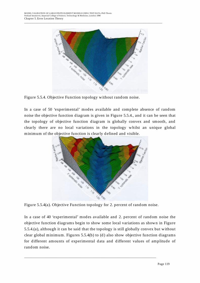
MODEL VALIDATION OF LARGE FINITE ELEMENT MODELS USING TEST DATA, PhD ThesisNedzad Imamovic, Imperial College of Science, Technology & Medicine, London 1998
Chapter 5. Error Location Theory__________________________________________________________________________________________
______________________________________________________________________________________
Page 119
Figure 5.5.4. Objective Function topology without random noise.
In a case of 50 ‘experimental’ modes available and complete absence of randomnoise the objective function diagram is given in Figure 5.5.4., and it can be seen thatthe topology of objective function diagram is globally convex and smooth, andclearly there are no local variations in the topology whilst an unique globalminimum of the objective function is clearly defined and visible.
Figure 5.5.4(a). Objective Function topology for 2. percent of random noise.
In a case of 40 ‘experimental’ modes available and 2. percent of random noise theobjective function diagrams begin to show some local variations as shown in Figure5.5.4.(a), although it can be said that the topology is still globally convex but withoutclear global minimum. Figures 5.5.4(b) to (d) also show objective function diagramsfor different amounts of experimental data and different values of amplitude ofrandom noise.

MODEL VALIDATION OF LARGE FINITE ELEMENT MODELS USING TEST DATA, PhD ThesisNedzad Imamovic, Imperial College of Science, Technology & Medicine, London 1998
Chapter 5. Error Location Theory__________________________________________________________________________________________
______________________________________________________________________________________
Page 120
Figure 5.5.4(b). Objective Function topology for 5. percent of random noise.
Figure 5.5.4(c). Objective Function topology for 10. percent of random noise.
Figure 5.5.4(d). Objective Function topology for 15. percent of random noise.
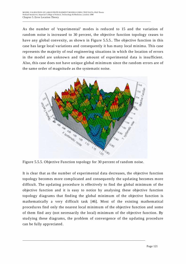
MODEL VALIDATION OF LARGE FINITE ELEMENT MODELS USING TEST DATA, PhD ThesisNedzad Imamovic, Imperial College of Science, Technology & Medicine, London 1998
Chapter 5. Error Location Theory__________________________________________________________________________________________
______________________________________________________________________________________
Page 121
As the number of ‘experimental’ modes is reduced to 15 and the variation ofrandom noise is increased to 30 percent, the objective function topology ceases tohave any global convexity, as shown in Figure 5.5.5.. The objective function in thiscase has large local variations and consequently it has many local minima. This caserepresents the majority of real engineering situations in which the location of errorsin the model are unknown and the amount of experimental data is insufficient.Also, this case does not have unique global minimum since the random errors are ofthe same order of magnitude as the systematic noise.
Figure 5.5.5. Objective Function topology for 30 percent of random noise.
It is clear that as the number of experimental data decreases, the objective functiontopology becomes more complicated and consequently the updating becomes moredifficult. The updating procedure is effectively to find the global minimum of theobjective function and it is easy to notice by analysing these objective functiontopology diagrams that finding the global minimum of the objective function ismathematically a very difficult task [46]. Most of the existing mathematicalprocedures find only the nearest local minimum of the objective function and someof them find any (not necessarily the local) minimum of the objective function. Bystudying these diagrams, the problem of convergence of the updating procedurecan be fully appreciated.
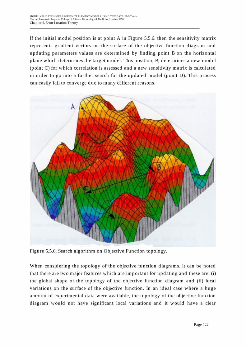
MODEL VALIDATION OF LARGE FINITE ELEMENT MODELS USING TEST DATA, PhD ThesisNedzad Imamovic, Imperial College of Science, Technology & Medicine, London 1998
Chapter 5. Error Location Theory__________________________________________________________________________________________
______________________________________________________________________________________
Page 122
If the initial model position is at point A in Figure 5.5.6. then the sensitivity matrixrepresents gradient vectors on the surface of the objective function diagram andupdating parameters values are determined by finding point B on the horizontalplane which determines the target model. This position, B, determines a new model(point C) for which correlation is assessed and a new sensitivity matrix is calculatedin order to go into a further search for the updated model (point D). This processcan easily fail to converge due to many different reasons.
Figure 5.5.6. Search algorithm on Objective Function topology.
When considering the topology of the objective function diagrams, it can be notedthat there are two major features which are important for updating and these are: (i)the global shape of the topology of the objective function diagram and (ii) localvariations on the surface of the objective function. In an ideal case where a hugeamount of experimental data were available, the topology of the objective functiondiagram would not have significant local variations and it would have a clear
MODEL VALIDATION OF LARGE FINITE ELEMENT MODELS USING TEST DATA, PhD ThesisNedzad Imamovic, Imperial College of Science, Technology & Medicine, London 1998
Chapter 5. Error Location Theory__________________________________________________________________________________________
______________________________________________________________________________________
Page 123
convex (or concave, depending on the reference point) shape. In most practical caseswhere an incomplete set of experimental data is used for updating, the globalconvex shape cannot be recognised due to the dominance of the large localvariations. One way of making the topology of objective function globally moreconvex is by including experimental data which have higher residuals (hereresiduals means the difference between measured and predicted values) in theupdating equation. Completely the opposite approach is to use only experimentaldata which have low residuals in order to improve the convergence process of theupdating process, but in fact this localises the objective function topology andprovides only minor improvement to the initial model. It can be concluded that it isequally important to include even experimental mode shapes which do not initiallycorrelate well with any modes from the theoretical model in order to make theobjective function diagram globally more convex, although this can numericallydestabilise the updating process. This also leads to a conclusion that it is importantto find positions which would detect possible discrepancies between theexperimental and theoretical models, rather than measure only at positions whichwould indicate low degree of disagreement and make the objective functiondiagram globally less convex with large local variations.
5.5.1. Random Errors Distribution Theory
It has been demonstrated in the previous section that the amount of experimentaldata available has an important role in the whole updating process. The fewerexperimental data that are available, the more complicated the objective functiondiagram is. These diagrams provide good visual representation of the updatingprocess. One approach for complete updating is to generate the objective functiondiagram using as much experimental data as possible and then simply to findregions of minimum value of the objective function. Unfortunately, this processrequires a huge calculation effort, even for a very simple finite element model witha small number of DOFs.
Random errors distribution theory assumes that every parameter in a finite elementmodel is inaccurate and that the errors of the parameters are random values whichare limited. These limits have different values for different parameters and theanalyst should be able to select groups of finite element parameters of equivalenterror limits. For instance, the node positions are probably uncertain up to 0.05 % ofthe largest dimension of a structure while the stiffness values of some elements are
MODEL VALIDATION OF LARGE FINITE ELEMENT MODELS USING TEST DATA, PhD ThesisNedzad Imamovic, Imperial College of Science, Technology & Medicine, London 1998
Chapter 5. Error Location Theory__________________________________________________________________________________________
______________________________________________________________________________________
Page 124
uncertain up to 50 % of the original values. In this example, it is clear that thedominant uncertainty comes from the stiffness values and they are the ones thatshould be selected as updating parameters. This quantification process of thedetermination of the uncertainty limits for different updating parameters is alsodependent on the correlation results. The better the correlation result, the moredifficult it is to determine the error limits for different finite element parameters. Asthe correlation improves, it is possible to arrive at a stage where correlation could beexplained by the mistuning effect for some structures rather than any errors in amodel. In most practical situations this possibility can be ruled out since theagreement between the predicted and measured properties is so low that themistuning effect is not considered to be a reasonable explanation for discrepancies.
Determination of uncertainty limits is a part of the empirical selection of updatingparameters [1] and the random errors distribution theory is used to explain and tounderstand that selection process which is visualised through objective functiondiagrams.
5.6. Conclusions
The clear conclusion of the above discussion is that it is generally impossible toupdate a structure uniquely when only a limited amount of experimental data areavailable and instead only a partial error localisation can be attempted. In order tolocalise errors further, the elements which are found to be responsible fordiscrepancies should be refined, i.e. these elements should be separated into anumber of parameters in order to allocate errors more accurately. Also, this processwould increase the number of updating parameters and consequently the datarequirements for updating would increase proportionally. Objective functiondiagrams clearly show what impact data requirements have on model updatingsuccess. Also, these diagrams show the complexities and difficulties which liebehind the updating task in general. Nevertheless, since direct model identificationis impossible, because the inaccessible higher modes contribute mostly to stiffnessmatrix, model updating is currently the best available approach for obtainingtheoretical models of improved accuracy.

MODEL VALIDATION OF LARGE FINITE ELEMENT MODELS USING TEST DATA, PhD ThesisNedzad Imamovic, Imperial College of Science, Technology & Medicine, London 1998
Chapter 6. Model Updating__________________________________________________________________________________________
------------------------------------------------------------------------------------------------------------------------------------------Page 125
6.0 Model Updating
6.1. Introduction
Model updating can be defined as the process of correcting an original finiteelement model in order to improve correlation with experimental data. Onceexperimental data are collected, an initial correlation is performed and the updatingparameters are selected, and it becomes necessary to choose an updating approachthat will minimise the discrepancies between the experimental and the updatedmodels. There are several different mathematical updating procedures developedspecifically to minimise discrepancies between the two models. These proceduresare based on different assumptions and mathematically they may be quite different,but they all have one common feature and that is minimisation of an objectivefunction.
Until recently, model updating was considered to be the complete procedure forfinding an accurate model of a particular system in structural dynamics. Theproblem of finding this accurate model has been considered from a broadperspective using both empirical and theoretical knowledge about the dynamicbehaviour of linear structures, in which even the accuracy of experimental data wasquestioned. By combining existing research methods and theories from this area,several conclusions were drawn in the previous chapters. One is that it is impossibleto carry out a complete identification of structural model parameters; and thisinfluenced the course of research in the area of model validation. Much previouswork has concentrated solely on model updating considering correlation and datarequirements as being of secondary importance. Structural dynamic researchers arecontinuously producing yet more new updating approaches, but little or noattention is paid to areas that are considered to be outside the research scope but infact appear to be fundamental, such as the selection of updating parameters andexperimental data requirements [47].
This chapter provides an introduction to existing updating formulations and theirincorporation in the model validation process together with the new methods forcorrelation, updating parameter selection and data requirements presented earlier.Although model updating is an important part of the model validation process, it isnot possible to quantify its relative role in comparison with the other parts of themodel validation process. Model updating provides a mathematical procedure formodel parameter identification of already-selected updating parameters and

MODEL VALIDATION OF LARGE FINITE ELEMENT MODELS USING TEST DATA, PhD ThesisNedzad Imamovic, Imperial College of Science, Technology & Medicine, London 1998
Chapter 6. Model Updating__________________________________________________________________________________________
------------------------------------------------------------------------------------------------------------------------------------------Page 126
measured experimental data. Most updating approaches are, in effect, linearisationof a complicated mathematical function, i.e. dynamics properties are approximatedas linear function of updating parameters. The model updating task is to find theglobal minimum of an objective function which is defined mainly by selectedupdating parameters and measured experimental data and partly by mathematicalformulation of an updating method. Whether the final updating equation isoverdetermined or underdetermined, the search algorithm will be decided by themathematical formulation of the updating method.
6.1.1. Definition of The Updated Model
Defining the updated model of a structure is as difficult as the updating processitself. If m experimental mode shapes have been measured at n DOFs, then amathematical definition of the updated model is contained in the followingexpression:
λ rA = λ r
E , r = 1,... ,m (6.1.1-1)
φ j ,rA = φ j ,r
E , r = 1,...,m; j = 1,. ..,n (6.1.1-2)
or a more complete requirement is that the responses must satisfy the following:
α jA ω( )= α j
E ω( ), 0 ≤ ω ≤ ∞; j = 1,...,n (6.1.1-3)
The above expressions are necessary conditions for an updated model to be the
updated model but whether they are sufficient is not known. This depends on therelative amount of experimental data available and that in turn is determined by themodal test planning procedure. Moreover, the modal test planning procedureassumes that at least the frequency range for the experiments is known and isdetermined by the final use of the updated model. For instance, if the updatedmodel is to be used for general linear transient response predictions then there is asimple relationship between the minimum transient analysis time step and thefrequency range in which the dynamic behaviour of the updated model should bevalidated. This procedure is described in section 2.2.3. If, however, the updatedmodel is to be used for a linear static analysis then there is no need to attempt tocorrelate high-frequency responses; it is important that there is good correlation ofFRFs in the low-frequency range only.

MODEL VALIDATION OF LARGE FINITE ELEMENT MODELS USING TEST DATA, PhD ThesisNedzad Imamovic, Imperial College of Science, Technology & Medicine, London 1998
Chapter 6. Model Updating__________________________________________________________________________________________
------------------------------------------------------------------------------------------------------------------------------------------Page 127
The requirement (6.1.1-3) may seem a complete condition for two models to beequivalent (equivalent FRFs). However, it is still only a limited number of FRFs thatare included in (6.1.1-3) and therefore this condition is only extended from theconditions (6.1.1-1 and -2) for correlation of damping values.Since it is possible to measure only a limited amount of experimental data, it can beconcluded that defining the updated model is not possible. Instead, it isrecommended to define the final use of the updated model and from that to identifythe frequency range for the validation process. Even if measurement of an unlimitedamount of data were possible, it is hard to believe that any numerical model whichconsists of mass, stiffness and damping matrices would be able to reproduce all theexperimental data exactly. Although it is a highly sensitive area for discussion, itwill be concluded here that the updated model does not exist and instead that it isonly possible to identify an updated model that is very close to something that weconsider as the updated model. Defining the criteria for determination of minimumdata requirements for updating is the next step forward in the updating processitself.
6.2. Classification of Updating Methods
Existing updating methods can be classified into two major groups according theform of the experimental data they use, [47], and these are: (i) methods that usemodal domain data and (ii) methods that use frequency domain data. The aim ofthis thesis is not to review all existing methods, or to list them here for educationalpurposes, but rather to concentrate on the in-depth research of some methods thatcurrently seem to be most promising for use on large finite element models.
6.2.1. Modal-domain updating methods
Modal-domain updating methods can be further subdivided into (a) direct and (b)iterative updating methods.
Direct modal-domain updating methods do not require an iterative process to find theupdated model and this feature avoids excessive computation and the possibility ofdivergence. A major weakness of this type of updating method is that although itreproduces the measured data exactly and there is no possibility of selection of
MODEL VALIDATION OF LARGE FINITE ELEMENT MODELS USING TEST DATA, PhD ThesisNedzad Imamovic, Imperial College of Science, Technology & Medicine, London 1998
Chapter 6. Model Updating__________________________________________________________________________________________
------------------------------------------------------------------------------------------------------------------------------------------Page 128
updating parameters, i.e. only whole-matrix updating is possible. The exactreproduction of the measured data is a weakness because if there is any noise in themeasured data the noise will be reproduced too. One particular problem with thesemethods is that they require a full set of the measured mode shapes and as a resultthese methods will not be selected for further research of updating of large finiteelement models.
Iterative modal-domain updating methods use some iterative procedure to minimise aparticular objective function which is defined using some correlation parameters. Amajor weakness of these updating methods is that they require the iterative processto update the initial model and there is no guarantee of convergence. Anotherproblem is that they require accurate pairing of the correlated modes at everyiteration. The main strength of these methods is that they allow a wide choice ofupdating parameters and experimental data as well as selective weighting on both.These methods do not require inclusion of damping in the model. Also, the mostimportant feature of these methods is that they do not require complete modeshapes for updating and, and as result, they will be selected for further research ofupdating of large finite element models.
6.2.2. Frequency-domain updating methods
Frequency-domain updating methods use the measured frequency responsefunction data directly so there is no need for modal analysis on the experimentaldata. The main weakness of these methods is that they require damping to beconsidered and this is very difficult to model accurately. Another difficulty withthese methods is that they require residual-free regenerated FRFs during theupdating process and the FOREST technique was specifically designed to tackle thisproblem. The process of selection of frequency points can be difficult if the initialcorrelation of natural frequencies is not particularly close. The selection of differentupdating parameters is allowed. These methods are generally considered to be notas effective as the iterative modal domain updating methods, but they could beused for updating of large finite element models.
6.3. Application of Linear Regression Theory to Model Updating
Linear regression theory [48][9][49] has an important application in most modelupdating approaches and therefore a thorough understanding of this theory is

MODEL VALIDATION OF LARGE FINITE ELEMENT MODELS USING TEST DATA, PhD ThesisNedzad Imamovic, Imperial College of Science, Technology & Medicine, London 1998
Chapter 6. Model Updating__________________________________________________________________________________________
------------------------------------------------------------------------------------------------------------------------------------------Page 129
crucial. The basic equation of most model updating approaches is the same as thestandard linear regression equation, i.e. of the following form:
S[ ]Noxl ∆p{ }l+ ε{ }No
= ∆W{ }No(6.3-1)
where S[ ]Noxl is the matrix of predictors, [50], ε{ }No is a vector of unknown random
disturbances, ∆W{ }No is the vector of observations and ∆p{ }
l is a vector of updating
parameters. The number of rows in the updating equation is No - the number of
observations, while the number of columns is l - the number of updatingparameters. The ratio between the number of observations, No , and the number of
updating parameters, l , will determine whether the updating equation isoverdetermined or underdetermined. The updating equation will beoverdetermined if the following condition is true:
No > l (6.3-2)
whereas the underdetermined updating equation is defined for the followingcondition,
No < l (6.3-3)
and a determined updating equation is defined when the following is satisfied,
No = l (6.3-4)
although the case of the determined updating equation is not equivalent to eitherthe overdetermined or underdetermined case, and has some properties of bothprocesses. Mathematically, there is a fundamental difference in the processes ofsolving and interpretation between overdetermined and underdetermined updatingequations and therefore these two cases will be considered separately, [51][49].
Overdetermined Updating Equation
When the number of observations is larger than the number of updating parametersin the updating equation then the updating equation is said to be overdetermined.There is not always an exact solution for (6.3-1) such that all equations are satisfied.Instead, a solution of the (6.3-1) equation is defined as a vector of updating
MODEL VALIDATION OF LARGE FINITE ELEMENT MODELS USING TEST DATA, PhD ThesisNedzad Imamovic, Imperial College of Science, Technology & Medicine, London 1998
Chapter 6. Model Updating__________________________________________________________________________________________
------------------------------------------------------------------------------------------------------------------------------------------Page 130
parameters, ∆ˆ p { }l, such that the following norm of the residual vector, ∆r{ } is
minimised:
∆r{ }T ∆r{ }= ∆W{ }No− S[ ]Noxl ∆p{ }
l( )T
∆W{ }No− S[ ]Noxl ∆p{ }
l( ) (6.3-5)
It is important to mention here that an overdetermined updating equation has aunique solution under some conditions, i.e. there is only one solution of equation(6.3-1) which minimises the residual vector. The least-squares procedure for findingthe solution vector in this case, ∆ˆ p { }
l, and the necessary conditions for the existence
of the unique solution, will be described in section (6.3.1).
Underdetermined Updating Equation
When the number of independent observations is smaller than the number ofupdating parameters then the updating equation is said to be underdetermined andthere are an infinite number of different vectors, ∆ˆ p { }
l, which make the updating
equation (6.3-1) fully satisfied. The problem encountered in this case is that there isno unique solution of the updating equation and that requires a special treatmentfor estimating updating parameters. One method which determines a uniquesolution of an underdetermined equation is the Singular Value Decomposition, [9].A solution of equation (6.3-1) found using the Singular Value Decompositionmethod is particularly interesting in model updating because it defines a solutionvector, ∆ˆ p { }
l, that has a minimum norm amongst all possible solutions. The
Singular Value Decomposition method and its application in model updating willbe described in more detail in section (6.3.2).
6.3.1. Least-Squares Method
The standard least-squares problem is defined in expression (6.3-1) for the case ofan overdetermined system of equations. The least-squares of vector ∆p{ }
l is
obtained by minimising the norm of the residual vector defined in (6.3-5). Takingthe first derivative of (6.3-5) with respect to ∆p{ }
l yields the so-called normal
equations:
S[ ]TS[ ]( ) ∆p{ } = S[ ]T ∆W{ } (6.3.1-1)

MODEL VALIDATION OF LARGE FINITE ELEMENT MODELS USING TEST DATA, PhD ThesisNedzad Imamovic, Imperial College of Science, Technology & Medicine, London 1998
Chapter 6. Model Updating__________________________________________________________________________________________
------------------------------------------------------------------------------------------------------------------------------------------Page 131
The system of linear equations (6.3.1-1) has a unique solution if, and only if, theinverse of S[ ]T
S[ ]( ) exists. In this case, the least-squares estimate of ∆p{ }l is
∆ˆ p { }= S[ ]TS[ ]( )−1
S[ ]T ∆W{ } (6.3.1-2)
This least-squares estimate ∆ˆ p { }l has several features if, and only if, certain
assumptions described hold [48], and these features are:
(i) E ∆ ˆ p { }l[ ]= ∆p{ }
l(6.3.1-3)
that is, ∆ˆ p { }l is an unbiased estimate for ∆p{ }
l.
(ii) Var ∆ ˆ p { }( )= σ 2 S[ ]TS[ ]( )−1
(6.3.1-4)
∆ˆ p { }l is the best linear unbiased estimate for ∆p{ }
l, that is, among the
class of linear unbiased estimates, ∆ˆ p { }l has the smallest variance.
(iii) ∆ˆ p { }∝ Νl ( ∆p{ },σ 2 S[ ]TS[ ]( )−1
) (6.3.1-5)
where Ν l(µ, Σ) denotes an l -dimensional normal distribution with
mean µ and variance Σ .
The vector of fitted (predicted) values is given by:
∆ ˆ W { }= S[ ] ∆ ˆ p { } = S[ ] S[ ]TS[ ]( )−1
S[ ]T ∆W{ }= P[ ] ∆W{ } (6.3.1-6)
where the so-called ‘prediction’ matrix,
P[ ]= S[ ] S[ ]T S[ ]( )−1S[ ]T (6.3.1-7)
has the following properties:
(iv) E ∆ ˆ W { }[ ]= S[ ] ∆p{ } (6.3.1-8)
(v) Var ∆ ˆ W { }( )= σ 2 P[ ] (6.3.1-9)
(vi) ∆ ˆ W { }∝ NNo( S[ ] ∆p{ },σ 2 P[ ]) (6.3.1-10)
MODEL VALIDATION OF LARGE FINITE ELEMENT MODELS USING TEST DATA, PhD ThesisNedzad Imamovic, Imperial College of Science, Technology & Medicine, London 1998
Chapter 6. Model Updating__________________________________________________________________________________________
------------------------------------------------------------------------------------------------------------------------------------------Page 132
The vector of ordinary residuals, ∆e{ }, which is defined as
∆e{ } = ∆W{ }− ∆ ˆ W { }= ∆W{ }− P[ ] ∆W{ } = I[ ]− P[ ]( ) ∆W{ } (6.3.1-11)
has the following properties [48]:
(vii) E ∆e{ }[ ]= 0{ } (6.3.1-12)
(viii) Var ∆e{ }( )= σ2 I[ ]− P[ ]( ) (6.3.1-13)
(ix) ∆e{ } ∝ NNo( 0{ },σ 2 I[ ]− P[ ]( )) (6.3.1-14)
An unbiased estimate of σ 2 is given by
(x) ˆ σ 2 =∆e{ }T ∆e{ }
No − l=
∆W{ }T I[ ]− P[ ]( ) ∆W{ }No − l
(6.3.1-15)
The above results (i)-(x) are valid only if the following assumptions hold [48].
1. Linearity assumption: This assumption is implicit in the definition of equation (6.3-1) which says that each observed response value ∆Wi can be written as a linearfunction of the i-th row of S[ ], S{ }i
T , that is,
∆Wi = S{ }i
T ∆p{ }+ ε i , i = 1,. .., No (6.3.1-16)
2. Computational assumption: In order to find a unique estimate of ∆p{ }l it is
necessary that S[ ]TS[ ]( )−1
exists, or equivalently that:
rank S[ ]( )= l (6.3.1-17)
3. Distributional assumption: The statistical analyses based on least-squares (e.g., thet-test, the F-test, etc.) assume that
(a) S[ ] is without errors, (6.3.1-18)
(b) ε i does not depend on S{ }i
T, i = 1,... , No , and (6.3.1-19)
(c) ε{ }∝ NNo( 0{ },σ 2 I[ ]) (6.3.1-20)
MODEL VALIDATION OF LARGE FINITE ELEMENT MODELS USING TEST DATA, PhD ThesisNedzad Imamovic, Imperial College of Science, Technology & Medicine, London 1998
Chapter 6. Model Updating__________________________________________________________________________________________
------------------------------------------------------------------------------------------------------------------------------------------Page 133
4. Implicit assumption: All observations are equally reliable and should have an equalrole in determining the least-squares results and influencing conclusions.
Not all of these assumptions are required in all situations. For example, for (6.3.1-3)to be valid, the following assumptions must hold: (6.3.1-16), (6.3.1-17), (6.3.1-18) andpart of (6.3.1-20), that is, Ε ε{ }[ ]= 0{ }. On the other hand, for (6.3.1-4) to be correct,
assumption (6.3.1-19), in addition to the above assumptions, must hold.
6.3.2. Singular Value Decomposition
The singular value decomposition (SVD) of matrix S[ ] is defined in the following
expression [9]:
U[ ]No xNo
TS[ ]No xl V[ ]lxl = Σ[ ]pxp
(6.3.2-1)
where Σ[ ]pxp = diag σ1 ,σ2 , ...,σ p[ ] (6.3.2-2)
p = min No ,l( ) (6.3.2-3)
and σ1 ≥ σ2 ≥...≥ σ p > 0 (6.3.2-4)
The values σ j , j = 1,... , p are the singular values of S[ ]. The matrices U[ ] and V[ ]satisfy the following condition:
U[ ]*U[ ] = V[ ]*
V[ ] = I[ ] (6.3.2-5)
Using the (6.3.2-5) condition it is straightforward to find the pseudo-inverse to begiven by
S[ ]lxNo
+ = V[ ]lxl
Σpxp−1 0
0 0
lxN0
U[ ]NoxN o
T(6.3.2-6)
MODEL VALIDATION OF LARGE FINITE ELEMENT MODELS USING TEST DATA, PhD ThesisNedzad Imamovic, Imperial College of Science, Technology & Medicine, London 1998
Chapter 6. Model Updating__________________________________________________________________________________________
------------------------------------------------------------------------------------------------------------------------------------------Page 134
The condition number of a matrix S[ ] is defined [52] as
cond( S[ ]) =max
x{ }
S[ ] x{ }x{ }
minx{ }
S[ ] x{ }x{ }
(6.3.2-7)
which, in the case of known singular values of the full rank matrix S[ ], becomes
cond( S[ ]) = κ =σmax
σmin
(6.3.2-8)
The condition number of a matrix can be used to assess how close the matrix is tosingularity. Matrices with small values of the condition number are said to be well-conditioned while matrices with large condition number are said to be ill-conditioned. It is difficult to define the exact value of the condition number thatseparates well- and ill-conditioned matrices, but for a sufficient number of digits ofcomputation these values are: (i) κ < 105 defines well-conditioned matrices, (ii)105 < κ < 108 defines ill-conditioned matrices and (iii) 108 < κ defines numericallysingular matrices [29][9]. These values should be taken as the order of magnitudeonly rather than as exact values. The condition number is generally used forassessment of the accuracy of solutions that are dependent on some inverse matricesrather than as a tool for pure assessment of singularity of a matrix. For more reliableand accurate ways of determination of the singularity and the rank of a matrix, thesingular value decomposition method is used as described below.
The rank of a matrix S[ ] is defined by the number of non-zero singular values of the
matrix, that is,
rank( S[ ]) = r, σmax ≥.. .≥ σ r ≥ σr +1 =...= σ p = 0 (6.3.2-9)
When a matrix contains noisy data it is possible to have some singular values whichare not identically zero but which are small enough to be taken as zero singularvalues of the matrix. In this situation it is necessary to define the numerical limit fordetermination of the singular values and the smallest value for determination of thesingular values is the computer threshold value, ATHRESHOLD, as defined in (2.2.1-3)
[52]. The threshold values for 8- and 16-digit machines are given in expressions(2.2.1-4) and (2.2.1-5). Therefore all singular values of a matrix that have the values

MODEL VALIDATION OF LARGE FINITE ELEMENT MODELS USING TEST DATA, PhD ThesisNedzad Imamovic, Imperial College of Science, Technology & Medicine, London 1998
Chapter 6. Model Updating__________________________________________________________________________________________
------------------------------------------------------------------------------------------------------------------------------------------Page 135
smaller than the appropriate threshold value will be considered to be zero andconsequently will not be counted for the rank of the matrix, i.e.,
σ1 ≥ σ2 ≥...≥ σ r > ATHRESHOLD > 0 (6.3.2-10)
The singular value decomposition has an important role in solving theunderdetermined least-square problem since the solution found using the SVD isunique in the sense that it represents the minimum norm solution. Proof of thisstatement can be found in several sources, [9][49][53][48].
6.3.3. Solutions of Overdetermined and Undetermined Linear Systems
There are two major versions of the final updating equation (6.3-1) and these are: (i)overdetermined updating equations as described by (6.3-2) and (ii)underdetermined updating equations as described by (6.3-3). The solutionprocedures for these two types require the use of mathematically different methodsand tools. Each of these two major types can be further divided into two subgroupsin respect of the rank and conditioning of the matrix of predictors in the updatingequation. Whilst determination of whether an updating equation is overdeterminedor underdetermined is clearly defined, it is not so straightforward to determinewhether a matrix is of full rank, ill-conditioned or singular. Each of these differentcases is considered below and an appropriate solution procedure is developed andproposed. There is a strong argument for a complete understanding of differentmathematical methods employed for solving the updating equation due to the needfor physical explanation of the obtained results and estimation of their accuracy.
Solving of overdetermined updating equations
The least-squares method is mainly used for solving overdetermined updatingequations. However, these equations can become ill-conditioned or singular and inthese situations an appropriate method has to be used in order to find the mostaccurate solution.

MODEL VALIDATION OF LARGE FINITE ELEMENT MODELS USING TEST DATA, PhD ThesisNedzad Imamovic, Imperial College of Science, Technology & Medicine, London 1998
Chapter 6. Model Updating__________________________________________________________________________________________
------------------------------------------------------------------------------------------------------------------------------------------Page 136
Normal equations
The general least-squares solution (6.3.1-2) is obtained by resolving the normalequations (6.3.1-1). This procedure will produce a unique solution for the updatingparameters if the following conditions hold; (6.3.1-16), (6.3.1-17), (6.3.1-18) and(6.3.1-20). All these conditions are generally fulfilled in model updating theory andpractice. The linearity condition (6.3.1-16) is applicable to small values of updatingparameters. The normal distribution assumption (6.3.1-20) is in line with modaltesting results as described in section 3.0. The matrix of predictors is measuredwithout any noise, as required in the condition (6.3.1-18). The only condition thatpartially determines the accuracy of the solution is the rank of the matrix ofpredictors requirement (6.3.1-17). Unfortunately, the fulfilment of this conditiondoes not guarantee an accurate solution of the least-squares problem using thenormal equations. To explain this let us consider expression (6.3.1-2) which givesthe solution based on normal equations. The solution is mainly dependent on the
existence of the S[ ]TS[ ]( )−1
matrix and its conditioning. There is a very basic
relationship between the condition of the S[ ] and S[ ]TS[ ]( ) matrices as stated in the
following expression [9],
cond S[ ]T S[ ]( )= cond S[ ]( ){ }2(6.3.3-1)
It turns out that the matrix S[ ]TS[ ]( ) often has a high condition number, so that no
matter how the normal equations are actually solved, errors in the data androundoff errors introduced during the solution are excessively magnified in thecomputed coefficients. The normal equations are not a recommended approach forthe general least-squares problem. The most reliable methods are based on matrixfactorisation using orthogonal matrices, such as Orthogonal Factorisation
approach, Householder Transformations or Singular Value Decomposition [9].Nevertheless, there are situations where the normal equations offer an advantageand it is tempting to use the normal equations when there are many moreobservations than updating parameters.
To summarise the importance of the condition number in solving a system of linearequations: relative numerical accuracy in the solution is proportional to relativeaccuracy in the coefficient matrix or the right-hand side, with constant of
MODEL VALIDATION OF LARGE FINITE ELEMENT MODELS USING TEST DATA, PhD ThesisNedzad Imamovic, Imperial College of Science, Technology & Medicine, London 1998
Chapter 6. Model Updating__________________________________________________________________________________________
------------------------------------------------------------------------------------------------------------------------------------------Page 137
proportionality as large as the condition number. This means that relative accuracyof the solution is of the following form [52]:
ε ∆p{ }( )= Ccond S[ ]( )ε ∆W( )εmach (6.3.3-2)
where C is a special constant (which is usually not larger than 1) and εmach is a
binary computer constant determined by the number of bits, [52]. Suppose that thecondition number of the sensitivity matrix is cond S[ ]( )= 10 6 and that we have a
binary computer with 24 bits in the fraction, then the numerical accuracy of thesolution of a system of linear equations would be ε ∆p{ }( )≈ 1062−24 = 10−2 , but the
accuracy of the solution using the normal equations would beε ∆p{ }( )≈ 10122−24 = 104 . The second approach in this example would lead to a
completely inaccurate solution and consequently it would probably causedivergence of the updating analysis.
Solving of underdetermined updating equation
Solving of underdetermined linear equations requires a totally different approach tothat of solving overdetermined linear equations. An underdetermined system oflinear equations has an infinite number of solutions, i.e. there is no unique solutionto the problem. Therefore, it is necessary to impose some other criteria in addition tothe updating equation in order to determine a unique solution. The most commoncondition imposed upon the solution is that the norm of the updating parameters isminimised, as described in the following equation:
J = min ∆p{ } (6.3.3-3)
Solution of the underdetermined system of linear equations using the SVD approachwill minimise the norm of the updating parameters [9]. The pseudo-inverse of thesensitivity matrix can be found using the SVD as described in equation (6.3.2-6). Theproper use of the SVD involves a tolerance reflecting the accuracy of the originaldata and the floating point arithmetic being used. Increasing the tolerance leads tolarger residuals but gives results that are less likely to be sensitive to errors in theobservation data. Decreasing the tolerance leads to smaller residuals and givesresults that are more sensitive to the observation data. Neglecting singular values,σ i , less than the tolerance has the effect of decreasing the condition number. Since
the condition number is an error magnification factor, this results in a more reliable

MODEL VALIDATION OF LARGE FINITE ELEMENT MODELS USING TEST DATA, PhD ThesisNedzad Imamovic, Imperial College of Science, Technology & Medicine, London 1998
Chapter 6. Model Updating__________________________________________________________________________________________
------------------------------------------------------------------------------------------------------------------------------------------Page 138
determination of the updating parameters. The cost of this increased reliability is apossible increase in the size of the residuals.
6.4. Assessment of the Rank and the Conditioning of Updating Equation
In the previous section it was explained how to solve a general type of updatingequation, i.e. overdetermined or undetermined. If the updating equation isunderdetermined then the SVD algorithm must be employed and by choosing aproper tolerance for the minimum acceptable singular value it is possible to solvethe general updating equation even if the equation is ill-conditioned or singular. Ifthe updating equation is overdetermined but ill-conditioned or singular, then in thiscase the SVD has to be used in order to solve the updating equation with limitedaccuracy.
However, the SVD is not the only method of dealing with ill-conditioned or rank-deficient overdetermined updating equations. Another way of dealing with thesesituations is by proper selection of the updating parameters so that singularities ofthe updating equation are removed and/or the conditioning is improved [54]. Theminimum requirements for finding an accurate pseudo-inverse of the matrix ofpredictors is that the matrix is of full rank and well-conditioned. If, however, thematrix of predictors is rank-deficient or ill-conditioned, that means that somecolumns in the matrix are linearly dependent or almost linearly dependent,respectively. If this is the case, then identifying linearly-independent subsets ofcolumns in the matrix would enable the analyst to find a better fit for the updatingparameters by simply excluding those columns (this is equivalent to excluding someof the corresponding updating parameters) of the matrix that are responsible for therank-deficiency or the ill-conditioning.
Generally, in the problem of least-squares, this exclusion of linearly-dependentcolumns does not guarantee that the residual will be reduced but it does give asomewhat more stable and accurate solution. The fact that residuals are not affectedcan be explained by ill-conditioning and/or singularity of the matrix of predictorswhere the particular least-square problem does not have a unique solution, i.e. eventhough the system is overdetermined it has an infinite number of solutions that willproduce similar residuals. In these instances, the solution of the ill-conditionedleast-square problem tends to have large variances of extracted parameters and thisposes a major threat to physical justification of the obtained results. Therefore, it is

MODEL VALIDATION OF LARGE FINITE ELEMENT MODELS USING TEST DATA, PhD ThesisNedzad Imamovic, Imperial College of Science, Technology & Medicine, London 1998
Chapter 6. Model Updating__________________________________________________________________________________________
------------------------------------------------------------------------------------------------------------------------------------------Page 139
necessary to find an algorithm which can be used to identify a subspace of linearlyindependent columns from the matrix of predictors.
6.4.1. Identifying the Column Space of the Matrix of Predictors
Identifying the column space of the matrix of predictors is an extremely difficultprocess. Many publications have explored the problem and several procedures havebeen recommended for solving this problem and can be found in [55]. Therecommended methods are based on either the QR factorisation or the SVD andthey involve interchange strategy for identification of independent columns.Unfortunately, none of these procedure1 is guaranteed to succeed in finding thecolumn space of an ill-conditioned matrix in the general case, [55]. Hence, a newprocedure which consists of a continuing process for assessment of the contributionof each column to the conditioning of the matrix is constructed to resolve theproblem of identifying the column space of a matrix.
The final goal of this process of identification of the best subspace of a matrix is toidentify a set of columns of the matrix such that the condition of the matrix willhave a known value. Therefore, the value for the condition number is defined sothat when the matrix has a condition number less than or equal to that value, theprocess of identification of the column space will be stopped. The condition numberof the matrix is calculated using the SVD approach as described in (6.3.2-8)expression.
The following procedure can be employed for the identification of linearly-independent subspace of the overdetermined matrix of predictors:
(i) calculate the condition number for the following matrices,
κ i = cond Si( )[ ]
N0x (l-ξ-1)
i = 1,. .., l - ξ (6.4.1-1)
where the Si( )[ ]
N0x ( l-ξ-1) matrix is obtained by excluding the i-th column from the
S[ ]N0x( l -ξ ) matrix and the parameter ξ is the number of already excluded columns.
(1) 1 Q Zang, G Lallement, R Fillod, J Piranda “A Complete Procedure for Adjustment of a Mathematical Model from the
Identified Complex Modes” IMAC5, London, England 1987 (pp 1183 - 1190)
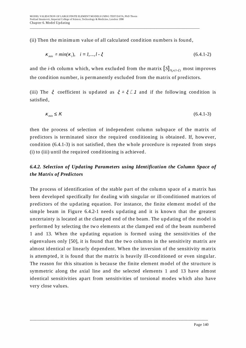
MODEL VALIDATION OF LARGE FINITE ELEMENT MODELS USING TEST DATA, PhD ThesisNedzad Imamovic, Imperial College of Science, Technology & Medicine, London 1998
Chapter 6. Model Updating__________________________________________________________________________________________
------------------------------------------------------------------------------------------------------------------------------------------Page 140
(ii) Then the minimum value of all calculated condition numbers is found,
κ min = min(κ i), i = 1,..., l - ξ (6.4.1-2)
and the i-th column which, when excluded from the matrix S[ ]N0x( l -ξ ) most improves
the condition number, is permanently excluded from the matrix of predictors.
(iii) The ξ coefficient is updated as ξ = ξ + 1 and if the following condition is
satisfied,
κ min ≤ Κ (6.4.1-3)
then the process of selection of independent column subspace of the matrix ofpredictors is terminated since the required conditioning is obtained. If, however,condition (6.4.1-3) is not satisfied, then the whole procedure is repeated from steps(i) to (iii) until the required conditioning is achieved.
6.4.2. Selection of Updating Parameters using Identification the Column Space of
the Matrix of Predictors
The process of identification of the stable part of the column space of a matrix hasbeen developed specifically for dealing with singular or ill-conditioned matrices ofpredictors of the updating equation. For instance, the finite element model of thesimple beam in Figure 6.4.2-1 needs updating and it is known that the greatestuncertainty is located at the clamped end of the beam. The updating of the model isperformed by selecting the two elements at the clamped end of the beam numbered1 and 13. When the updating equation is formed using the sensitivities of theeigenvalues only [50], it is found that the two columns in the sensitivity matrix arealmost identical or linearly dependent. When the inversion of the sensitivity matrixis attempted, it is found that the matrix is heavily ill-conditioned or even singular.The reason for this situation is because the finite element model of the structure issymmetric along the axial line and the selected elements 1 and 13 have almostidentical sensitivities apart from sensitivities of torsional modes which also havevery close values.
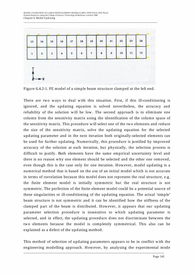
MODEL VALIDATION OF LARGE FINITE ELEMENT MODELS USING TEST DATA, PhD ThesisNedzad Imamovic, Imperial College of Science, Technology & Medicine, London 1998
Chapter 6. Model Updating__________________________________________________________________________________________
------------------------------------------------------------------------------------------------------------------------------------------Page 141
Figure 6.4.2-1. FE model of a simple beam structure clamped at the left end.
There are two ways to deal with this situation. First, if this ill-conditioning isignored, and the updating equation is solved nevertheless, the accuracy andreliability of the solution will be low. The second approach is to eliminate onecolumn from the sensitivity matrix using the identification of the column space ofthe sensitivity matrix. This procedure will select one of the two elements and reducethe size of the sensitivity matrix, solve the updating equation for the selectedupdating parameter and in the next iteration both originally-selected elements canbe used for further updating. Numerically, this procedure is justified by improvedaccuracy of the solution at each iteration, but physically, the selection process isdifficult to justify. Both elements have the same empirical uncertainty level andthere is no reason why one element should be selected and the other one removed,even though this is the case only for one iteration. However, model updating is anumerical method that is based on the use of an initial model which is not accuratein terms of correlation because this model does not represent the real structure, e.g.the finite element model is initially symmetric but the real structure is notsymmetric. The perfection of the finite element model could be a potential source ofthese singularities or ill-conditioning of the updating equation. The actual ‘simple’beam structure is not symmetric and it can be identified how the stiffness of theclamped part of the beam is distributed. However, it appears that our updatingparameter selection procedure is insensitive to which updating parameter isselected, and in effect, the updating procedure does not discriminate between thetwo elements because the model is completely symmetrical. This also can beexplained as a defect of the updating method.
This method of selection of updating parameters appears to be in conflict with theengineering modelling approach. However, by analysing the experimental mode
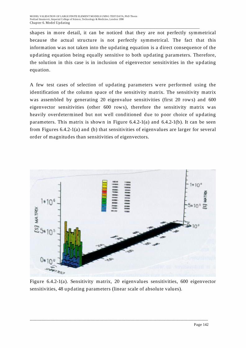
MODEL VALIDATION OF LARGE FINITE ELEMENT MODELS USING TEST DATA, PhD ThesisNedzad Imamovic, Imperial College of Science, Technology & Medicine, London 1998
Chapter 6. Model Updating__________________________________________________________________________________________
------------------------------------------------------------------------------------------------------------------------------------------Page 142
shapes in more detail, it can be noticed that they are not perfectly symmetricalbecause the actual structure is not perfectly symmetrical. The fact that thisinformation was not taken into the updating equation is a direct consequence of theupdating equation being equally sensitive to both updating parameters. Therefore,the solution in this case is in inclusion of eigenvector sensitivities in the updatingequation.
A few test cases of selection of updating parameters were performed using theidentification of the column space of the sensitivity matrix. The sensitivity matrixwas assembled by generating 20 eigenvalue sensitivities (first 20 rows) and 600eigenvector sensitivities (other 600 rows), therefore the sensitivity matrix washeavily overdetermined but not well conditioned due to poor choice of updatingparameters. This matrix is shown in Figure 6.4.2-1(a) and 6.4.2-1(b). It can be seenfrom Figures 6.4.2-1(a) and (b) that sensitivities of eigenvalues are larger for severalorder of magnitudes than sensitivities of eigenvectors.
Figure 6.4.2-1(a). Sensitivity matrix, 20 eigenvalues sensitivities, 600 eigenvectorsensitivities, 48 updating parameters (linear scale of absolute values).
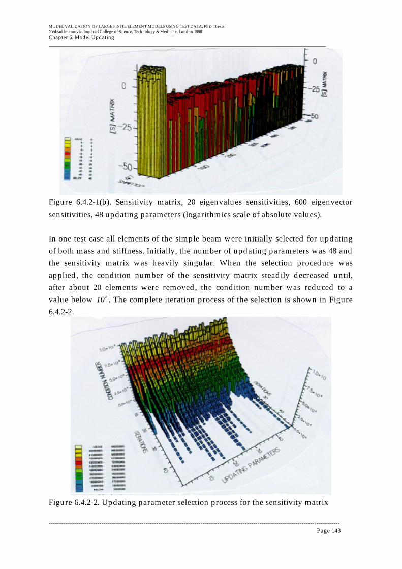
MODEL VALIDATION OF LARGE FINITE ELEMENT MODELS USING TEST DATA, PhD ThesisNedzad Imamovic, Imperial College of Science, Technology & Medicine, London 1998
Chapter 6. Model Updating__________________________________________________________________________________________
------------------------------------------------------------------------------------------------------------------------------------------Page 143
Figure 6.4.2-1(b). Sensitivity matrix, 20 eigenvalues sensitivities, 600 eigenvectorsensitivities, 48 updating parameters (logarithmics scale of absolute values).
In one test case all elements of the simple beam were initially selected for updatingof both mass and stiffness. Initially, the number of updating parameters was 48 andthe sensitivity matrix was heavily singular. When the selection procedure wasapplied, the condition number of the sensitivity matrix steadily decreased until,after about 20 elements were removed, the condition number was reduced to avalue below 105 . The complete iteration process of the selection is shown in Figure6.4.2-2.
Figure 6.4.2-2. Updating parameter selection process for the sensitivity matrix

MODEL VALIDATION OF LARGE FINITE ELEMENT MODELS USING TEST DATA, PhD ThesisNedzad Imamovic, Imperial College of Science, Technology & Medicine, London 1998
Chapter 6. Model Updating__________________________________________________________________________________________
------------------------------------------------------------------------------------------------------------------------------------------Page 144
consistsing of 20 eigenvalue sensitivities and 600 eigenvector sensitivities. Theinitial number of updating parameters was 48 (24 stiffness and 24 mass elements).A similar test case was performed for updating of the mass and stiffness elements ofthe same beam structure separately, and the result of that selection procedure isshown in Figure 6.4.2-3 and Figure 6.4.2-4, respectively. The iteration chart showsthat, for reasonable conditioning of the sensitivity matrix, at least half of allsymmetrical elements must be removed.
Figure 6.4.2-3. Updating parameter selection process for the sensitivity matrixconsistsing of 20 eigenvalue sensitivities and 600 eigenvector sensitivities. The initialnumber of updating parameters was 24 stiffness elements.
Figure 6.4.2-4. Updating parameter selection process for the sensitivity matrix

MODEL VALIDATION OF LARGE FINITE ELEMENT MODELS USING TEST DATA, PhD ThesisNedzad Imamovic, Imperial College of Science, Technology & Medicine, London 1998
Chapter 6. Model Updating__________________________________________________________________________________________
------------------------------------------------------------------------------------------------------------------------------------------Page 145
consistsing of 20 eigenvalue sensitivities and 600 eigenvector sensitivities. Theinitial number of updating parameters was 24 mass elements.
Use of cond S[ ]T S[ ]( ) for selection of updating parameters
One might think that in the process of finding the column space of the matrix ofpredictors it is possible to use S[ ]T
S[ ] rather than the S[ ] matrix (see expression
(6.3.3.-1)) in order to decrease the computational time required for calculation of thesingular values of the matrix. Figure 6.4.2-5 shows the difference of the conditionnumber estimates using the S[ ]T
S[ ] and S[ ] matrices, and it is clear that expression(6.3.3.-1) holds only for well-conditioned matrices. When the S[ ] matrix is ill-conditioned, then S[ ]T
S[ ] has twice as bad conditioning as the S[ ] matrix and the
estimate of the singular values of ill-conditioned and even worse conditionedmatrices are different. Because of this, the process of selection of updatingparameters is best performed using the S[ ] matrix rather than the S[ ]T
S[ ] matrix.
Figure 6.4.2-5. Updating parameter selection process for the matrix S[ ]TS[ ], where
the sensitivity matrix consistsing of 20 eigenvalue sensitivities and 600 eigenvectorsensitivities. The initial number of updating parameters was 48 (24 stiffness and 24mass elements).

MODEL VALIDATION OF LARGE FINITE ELEMENT MODELS USING TEST DATA, PhD ThesisNedzad Imamovic, Imperial College of Science, Technology & Medicine, London 1998
Chapter 6. Model Updating__________________________________________________________________________________________
------------------------------------------------------------------------------------------------------------------------------------------Page 146
6.5. Calculation of the Sensitivity Matrix
The sensitivity matrix consists of two different types of sensitivities; (i) eigenvaluesensitivities and (ii) eigenvector sensitivities. Definitions of both sensitivities aregiven in the two following sections, respectively.
6.5.1. Calculation of Eigenvalue Sensitivities
By differentiating expression (2.4-4) with respect to an updating parameter, it can beshown that eigenvalue sensitivity is given by the following expression:
∂λ Ar
∂pi
= φA{ }r
T ∂ KA[ ]∂pi
− λ Ar
∂ MA[ ]∂pi
φA{ } (6.5.1-1)
For mass or stiffness updating parameters defined as in expression (5.3) and (5.4),respectively, the eigenvalue mass or stiffness sensitivities are given in the followingexpressions, respectively:
∂λ Ar
∂p( M)i
= −λ Ar φA{ }r
TMA[ ]i
φ A{ }r
(6.5.1-2)
∂λ Ar
∂p( K)i
= φA{ }r
TKA[ ]i
φ A{ }r
(6.5.1-3)
6.5.2. Calculation of Eigenvector Sensitivities
Calculation of eigenvector sensitivities is more complicated than calculation ofeigenvector sensitivities. Fox and Kapoor (1968) derived the following expressionfor calculation of eigenvector mass and stiffness sensitivities for updatingparameters as defined in expressions (5.3) and (5.4), respectively:
∂ φA{ }r
∂p(M )i
= αrji
j =1
N
∑ φA{ }j
α rji = −
λ Ar φA{ }j
TMA[ ]
iφA{ }
r
λ Ar − λ Aj
r ≠ j( )
α rji = −
1
2φA{ }j
TMA[ ]i
φ A{ }rr = j( )
(6.5.2-1)
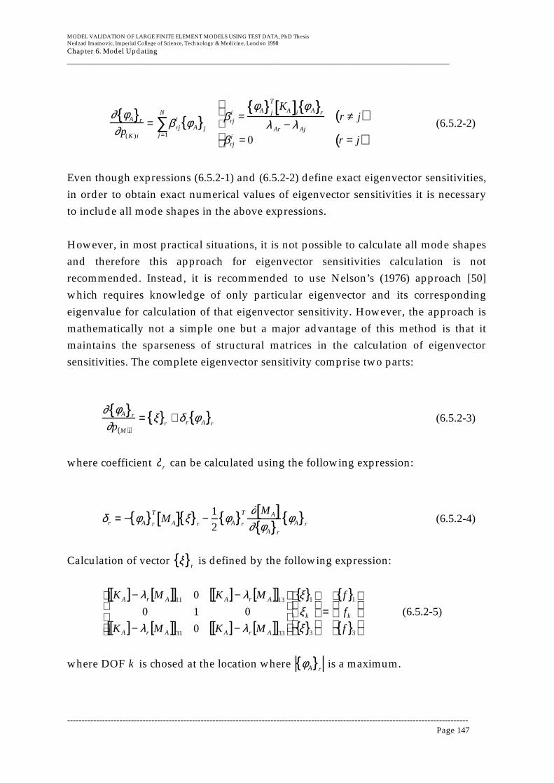
MODEL VALIDATION OF LARGE FINITE ELEMENT MODELS USING TEST DATA, PhD ThesisNedzad Imamovic, Imperial College of Science, Technology & Medicine, London 1998
Chapter 6. Model Updating__________________________________________________________________________________________
------------------------------------------------------------------------------------------------------------------------------------------Page 147
∂ φA{ }r
∂p(K )i
= β rji
j =1
N
∑ φ A{ }j
βrji =
φA{ }j
TKA[ ]i
φ A{ }r
λ Ar − λ Aj
r ≠ j( )
βrji = 0 r = j( )
(6.5.2-2)
Even though expressions (6.5.2-1) and (6.5.2-2) define exact eigenvector sensitivities,in order to obtain exact numerical values of eigenvector sensitivities it is necessaryto include all mode shapes in the above expressions.
However, in most practical situations, it is not possible to calculate all mode shapesand therefore this approach for eigenvector sensitivities calculation is notrecommended. Instead, it is recommended to use Nelson’s (1976) approach [50]which requires knowledge of only particular eigenvector and its correspondingeigenvalue for calculation of that eigenvector sensitivity. However, the approach ismathematically not a simple one but a major advantage of this method is that itmaintains the sparseness of structural matrices in the calculation of eigenvectorsensitivities. The complete eigenvector sensitivity comprise two parts:
∂ φA{ }r
∂p M( )i= ξ{ }
r+ δ r φ A{ }
r(6.5.2-3)
where coefficient δ r can be calculated using the following expression:
δ r = − φA{ }r
TMA[ ] ξ{ }
r−
1
2φA{ }
r
T ∂ MA[ ]∂ φA{ }r
φA{ }r
(6.5.2-4)
Calculation of vector ξ{ }r is defined by the following expression:
[ ] [ ][ ] [ ] [ ][ ]
[ ] [ ][ ] [ ] [ ][ ]
{ }
{ }
{ }
{ }
=
−−
−−
3
1
3
1
3331
1311
0
010
0
f
f
f
MKMK
MKMK
kk
ArAArA
ArAArA
ξξξ
λλ
λλ(6.5.2-5)
where DOF k is chosed at the location where φA{ }r
is a maximum.

MODEL VALIDATION OF LARGE FINITE ELEMENT MODELS USING TEST DATA, PhD ThesisNedzad Imamovic, Imperial College of Science, Technology & Medicine, London 1998
Chapter 6. Model Updating__________________________________________________________________________________________
------------------------------------------------------------------------------------------------------------------------------------------Page 148
The vector f{ }r is defined by the following expression:
f{ }r = −∂ K[ ]∂p
− λr
∂ M[ ]∂p
− φA{ }r
T ∂ K[ ]∂p
− λ r
∂ M[ ]∂p
φA{ }r M[ ]
φA{ }r(6.5.2-6)
Since it is not possible to calculate all mode shapes for the majority of practicalengineering applications, and particularly for large FE models, it is recommendedto use Nelson’s method for calculation of eigenvector sensitivities.
6.5.3. Use of Eigenvector Sensitivities
The sensitivity matrix of the FE model shown in Figure 6.4.2-1 consists of 620 rowsof which first 20 rows are eigenvalue sensitivities and the other 600 rows areeigenvector sensitivities. There are 12 updating parameters (stiffness values ofelements 1,2,..12), i.e. columns of sensitivity matrix. The rank of the sensitivitymatrix is 12 since the selection of updating parameters is such that all columns ofthe matrix are linearly independent because the condition number of this matrix iscond S[ ]620 x12( )= 139.58 . In this case, for a well-conditioned sensitivity matrix, it is
possible to calculate the prediction matrix of this sensitivity matrix in order to findthe contribution of every row to the rank of the matrix, as shown in the followingtable.

MODEL VALIDATION OF LARGE FINITE ELEMENT MODELS USING TEST DATA, PhD ThesisNedzad Imamovic, Imperial College of Science, Technology & Medicine, London 1998
Chapter 6. Model Updating__________________________________________________________________________________________
------------------------------------------------------------------------------------------------------------------------------------------Page 149
Row No. ModalParameter
Contributionto rank
1 λ , 0.2814323739792 x E-6
2 λ , 0.1096905701970 x E-3
3 λ , 0.6778407900804 x E-3
4 λ , 0.1274363632337 x E-2
5 λ , 0.1983045010151 x E-2
6 λ , 0.4173508823678 x E-1
7 λ , 0.7826221123678 x E-1
8 λ , 0.2894185810461
9 λ , 0.8396950191003
10 λ , 0.4443564606393
11 λ , 0.9987059873396
12 λ , 0.3737190949353
13 λ , 0.5400648100049
14 λ , 0.6575566689807
15 λ , 0.9021244756341
16 λ , 0.8945524503730
17 λ , 0.9679739606158
18 λ , 0.9837471523141
19 λ , 0.9948488605076
20 λ , 0.9891939575761
21 φ , 0.1018738100120 x E-11
22 φ , 0.4942650084504 x E-11
23 φ , 0.9146244241179 x E-12
24 φ , 0.9782250424170 x E-12
25 φ , 0.3566062058370 x E-11
26 φ , 0.2305001845271 x E-11
27 φ , 0.1802376582287 x E-11
28 φ , 0.2742710557550 x E-11
29 φ , 0.1161861234673 x E-11
30...620 φ ,... < 0.9 x E-11
Table 7. Contribution of eigenvalue and eigenvector sensitivities to the rank ofsensitivity matrix.

MODEL VALIDATION OF LARGE FINITE ELEMENT MODELS USING TEST DATA, PhD ThesisNedzad Imamovic, Imperial College of Science, Technology & Medicine, London 1998
Chapter 6. Model Updating__________________________________________________________________________________________
------------------------------------------------------------------------------------------------------------------------------------------Page 150
Also, in order to determine the contribution of the eigenvector sensitivities to thecondition number of the sensitivity matrix, let us consider the following study onthe same sensitivity matrix. If the first row of the sensitivity matrix is removediteratively, and the condition number recorded for every new reduced matrix, thenthe following results are obtained:
No. of EigenvalueSensitivities in [S]
matrixcond([S])
19 139.58
18 139.58
17 139.58
16 139.61
15 139.62
14 139.79
13 276.24
12 276.32
11 24539032.61
Table 8. Condition number of the sensitivity matrix as function of number ofeigenvalue sensitivities.
It is clear from Table 7 that contributions of the eigenvector sensitivities arenegligible in comparison with the eigenvalue sensitivities. It is also interesting tonote that sensitivities of higher eigenvalues are significantly more important thanthose of the lower eigenvalues. This observation is in line with conclusions obtainedin section 5.1.1. where the identification approach was discussed.
Considering the results presented in Table 8 it can be concluded that conditioning ofsensitivity matrix is independent of the inclusion of eigenvector sensitivities, i.e. theconditioning of the sensitivity matrix depends only on the number of eigenvaluesensitivities, the number of updating parameters and their selection. Anotherimportant conclusion from Table 8 is that the number of updating parametersshould not exceed the number of experimental natural frequencies.

MODEL VALIDATION OF LARGE FINITE ELEMENT MODELS USING TEST DATA, PhD ThesisNedzad Imamovic, Imperial College of Science, Technology & Medicine, London 1998
Chapter 6. Model Updating__________________________________________________________________________________________
------------------------------------------------------------------------------------------------------------------------------------------Page 151
The above results suggest that the inclusion of experimental mode shapes in thesensitivity matrix is not important, but it would be wrong to generalise thisstatement and suggest that it is not necessary to estimate experimental mode shapesat all because they cannot be used for sensitivity calculations and updating.Experimental mode shapes must be estimated because CMPs are selected byconsidering correlation between mode shapes, and even though it appears that theexperimental mode shapes do not have to be used in the updating equation directly,they still contribute to the updating equation through the selection of CMPs.However, it is possible to perform special weighting on the sensitivity matrix andincrease the contribution of eigenvector sensitivities to rank and conditioning of thesensitivity matrix as explained in the following section.
6.5.4. Weighting of the Sensitivity Matrix (Updating Equation)
Some researchers [45][19] perform a special weighting of the sensitivity matrix bymultiplying those rows which correspond to eigenvector sensitivities by largenumbers. This process will definitely give an extra importance to these rows, butthere is no physical justification for this particular weighting since the variance ofthe measured eigenvectors is several times larger than the variance of theeigenvalues. A statistically better weighting of the sensitivity matrix should beperformed by dividing each row of the matrix by the corresponding variance of thevariable used (eigenvalue or modal constant), but this weighting would furtherdecrease the importance of eigenvector sensitivities in the sensitivity matrix.
Also, it may be useful to use the COMAC correlation coefficient for weighting thesensitivity matrix, i.e. eigenvector sensitivities can be multiplied by the COMACvalue of the correponding DOF added to the value of a special constant εw −COMAC .
This weighting will increase the influence of DOFs which have good correlation anddecrease the influence of DOFs which have poor correlation measured by theCOMAC value. The coefficient εw −COMAC is a constant which is used to ensure that in
case of low COMAC value for a particular DOF, the contribution of this DOF to theobjective function is not completely diminished. For instance, let us consider twoDOFs which have COMAC values of 2% and 95%, respectively. The numericalcontribution to the objective function (error) of the first DOF (2 percent COMAC) isobviously much larger than the contribution of the second DOF (95 percentCOMAC). However, the sensitivities of the first DOF are more likely to be lessaccurate than the sensitivities of the second DOF due to less accurate modal
MODEL VALIDATION OF LARGE FINITE ELEMENT MODELS USING TEST DATA, PhD ThesisNedzad Imamovic, Imperial College of Science, Technology & Medicine, London 1998
Chapter 6. Model Updating__________________________________________________________________________________________
------------------------------------------------------------------------------------------------------------------------------------------Page 152
constants of first DOF than the second DOF, which is measured by COMAC values.It is difficult to recommend a particular value for the special constant, εw −COMAC , but
it should not be very small because, in this case, this weighting would removeinfluence of all major contributors to the objective function and the updatingequation would rely solely on only well correlated parameters. Too large a value ofthe special constant, εw −COMAC , would diminish the influence of the COMAC
coefficient and it would artificially force the updating solution to rely more onexperimental mode shapes rather than experimental eigenvalues even though thevariance on the measured mode shapes is larger than the variance on the measuredeigenvalues. The recommended values for εw −COMAC is to be in the range [0.1,100.].
6.6. Conclusions
Due to linear representation of the errors in the model, most model updatingmethods transform into a standard problem of least-squares. Several methods forsolving a general updating equation have been examined in this chapter, and it canbe concluded that in different situations different solution methods should be used.If there is large number of measured data and a small number of updatingparameters, then the use of normal equations seems to be the most suitable one.However, if the quantity of experimental data is only slightly greater than thenumber of updating parameters, then the SVD method should be used.
Use of eigenvector sensitivities has been discussed and it can be concluded thateigenvector sensitivities can be neglected, unless a special and largely unjustifiedweighting is performed (mulitiplying of eigenvector sensitivity rows with largevalues), and in order to keep updating equation well conditioned the number ofselected updating parameters should not exceed the number of experimentalnatural frequencies.
In any case, it is recommended to control conditioning and accuracy of theupdating equation by proper selection of the updating parameters as it is specifiedin a new method for selection for these parameters.

MODEL VALIDATION OF LARGE FINITE ELEMENT MODELS USING TEST DATA, PhD ThesisNedzad Imamovic, Imperial College of Science, Technology & Medicine, London 1998
Chapter 7. Model Validation Case Studies__________________________________________________________________________________________
------------------------------------------------------------------------------------------------------------------------------------------Page 153
7. Model Validation Case Studies
This chapter contains two practical model validation test cases. Each test case wascarefully chosen to highlight the applicability of model validation technology topractical engineering problems. The first case study is a simple cantilever beamclamped at one end. Even though the structure is extremely simple, the unknownclamped boundary condition make this example an interesting one, particularly as itwas selected as the benchmark for a validation study. The second case study is alarge aerospace structure for which a well-defined validation criterion is specified.This case study was selected to be presented here because it is a typical industrialexample, and the idea behind it is to show the real and practical challenges ananalyst will face when applying model validation technology to industrial cases.
7.1. Model Validation of Lloyd’s Register Structural Dynamics Correlation
Benchmark
7.1.1. Introduction
The Lloyd’s Register Structural Dynamics Correlation Benchmark structure consistsof three separate components: a cantilever beam, a baseplate and the foundation.The cantilever beam is firmly screwed to the baseplate which is resting on thefoundation. A detailed description of the benchmark can be found in Appendix 7Aand in reference [4].
7.1.2. FE model
The finite element model used for the structure consists of a shell element model ofthe cantilever beam partially embedded into a brick element model of the baseplate,as shown in Figure 3.6.5-5. Connection between the shell and brick parts of themodel is across the area shown in details in Figure 7-1. This overlap of shellelements inside the brick elements is necessary because the brick elements do nothave rotational degrees-of-freedom and a simple connection between shell and brickelements would treat the system as a mechanism. The specified thickness of the twobottom layers of shell elements is 1 mm only while the top layer connected to beamhas an equivalent thickness to that of the shell elements of the beam. The boundaryconditions specified in the model are free-free, as specified in the original
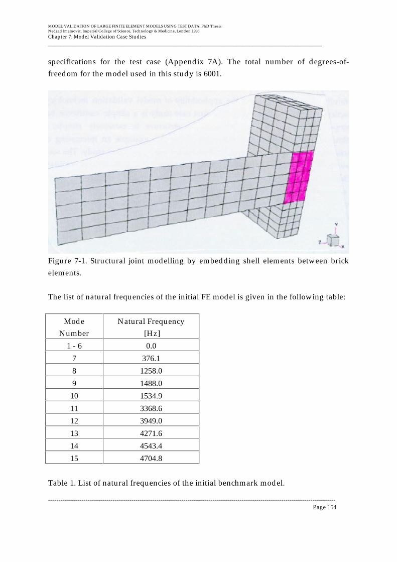
MODEL VALIDATION OF LARGE FINITE ELEMENT MODELS USING TEST DATA, PhD ThesisNedzad Imamovic, Imperial College of Science, Technology & Medicine, London 1998
Chapter 7. Model Validation Case Studies__________________________________________________________________________________________
------------------------------------------------------------------------------------------------------------------------------------------Page 154
specifications for the test case (Appendix 7A). The total number of degrees-of-freedom for the model used in this study is 6001.
Figure 7-1. Structural joint modelling by embedding shell elements between brickelements.
The list of natural frequencies of the initial FE model is given in the following table:
ModeNumber
Natural Frequency [Hz]
1 - 6 0.0
7 376.1
8 1258.0
9 1488.0
10 1534.9
11 3368.6
12 3949.0
13 4271.6
14 4543.4
15 4704.8
Table 1. List of natural frequencies of the initial benchmark model.
MODEL VALIDATION OF LARGE FINITE ELEMENT MODELS USING TEST DATA, PhD ThesisNedzad Imamovic, Imperial College of Science, Technology & Medicine, London 1998
Chapter 7. Model Validation Case Studies__________________________________________________________________________________________
------------------------------------------------------------------------------------------------------------------------------------------Page 155
7.1.3. Experimental data
The experimental data consisted of seven natural frequencies and quantitativedescriptions of the corresponding mode shapes. These data were supplied byLloyd’s Register who collected test results from three different companies whichcarried out the tests and also another set of natural frequencies was combined as theaverage results of all three supplied sets of data. Details of the original experimentaldata can be found in Appendix 7B. Close inspection of these data reveals thatdifferences in the measured natural frequency sets measured by different companiesare as high as 3 %. These differences could be considered as significant in terms ofreliability of the measured data but it is impossible to comment any further since noany additional information was supplied. In this case, it was decided to use averageresults from the three data sets since any systematic and/or random measurementerrors would be compensated in the average data set. As far as mode shapes areconcerned, only a basic geometric description was supplied by Lloyd’s Register andit will be necessary to assume that the experimental modes are symmetric. Themode shapes of the initial FE modes will be used as numerical values ofexperimental mode shapes for correlation purposes during updating process.
7.1.4. Correlation between experimental and initial FE results
Correlation between the experimental and initial FE models was performed bycomparing natural frequencies of two modes (one from the experimental and onefrom the initial FE model) which have the same mode shape description. Thefollowing table gives more details of this correlation of natural frequencies betweenexperimental and initial FE models.

MODEL VALIDATION OF LARGE FINITE ELEMENT MODELS USING TEST DATA, PhD ThesisNedzad Imamovic, Imperial College of Science, Technology & Medicine, London 1998
Chapter 7. Model Validation Case Studies__________________________________________________________________________________________
------------------------------------------------------------------------------------------------------------------------------------------Page 156
Exp.Mode
Av. Exp. Freq.[Hz]
Initial FEMode
Initial FE Freq.[Hz]
Relative Freq.Difference [%]
1 313 7 376.1 +20.2
2 1065 8 1258.0 +18.1
3 1210 10 1534.9 +26.9
4 1372 9 1488.0 +8.5
5 3019 11 3368.6 +11.6
6 3535 13 4271.6 +20.8
7 4250 14 4543.4 +6.9
Table 2. Correlation between Experimental and Initial FE models
7.1.5. Error localisation in FE model
Many errors in the initial FE model might be responsible for the discrepancies foundbetween the experimental and the initial FE models described in the previoussection. Some of these errors bear less and some more responsibility for theobserved discrepancies, but since in the description of the model it is said that thebaseplate and the beam are firmly screwed together it is probable that the maincauses of inaccuracy of the initial model are errors in this region of the model. Thereare probably some other errors as well, but the amount of the discrepancies causedby the other errors can probably be neglected in comparison with correlationdiscrepancies caused by the joint between the baseplate and the beam. The obviousconclusion from the above discussion is that most of the errors are assumed to beconcentrated at the joint between the baseplate and the cantilever beam and,consequently, the updating parameters will be selected in this region of thetheoretical FE model.
7.1.6. Updating of FE model
The selected method for updating was Inverse Eigensensitivity method mainly dueto the availability of only natural frequencies with quantitative description ofexperimental mode shapes only rather than any numerical values for them. Due tothis lack of experimental data it was possible to use only eigenvalue sensitivities formodel updating rather than combined sensitivity of both eigenvalues andeigenvectors.
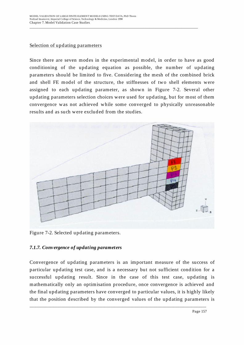
MODEL VALIDATION OF LARGE FINITE ELEMENT MODELS USING TEST DATA, PhD ThesisNedzad Imamovic, Imperial College of Science, Technology & Medicine, London 1998
Chapter 7. Model Validation Case Studies__________________________________________________________________________________________
------------------------------------------------------------------------------------------------------------------------------------------Page 157
Selection of updating parameters
Since there are seven modes in the experimental model, in order to have as goodconditioning of the updating equation as possible, the number of updatingparameters should be limited to five. Considering the mesh of the combined brickand shell FE model of the structure, the stiffnesses of two shell elements wereassigned to each updating parameter, as shown in Figure 7-2. Several otherupdating parameters selection choices were used for updating, but for most of themconvergence was not achieved while some converged to physically unreasonableresults and as such were excluded from the studies.
Figure 7-2. Selected updating parameters.
7.1.7. Convergence of updating parameters
Convergence of updating parameters is an important measure of the success ofparticular updating test case, and is a necessary but not sufficient condition for asuccessful updating result. Since in the case of this test case, updating ismathematically only an optimisation procedure, once convergence is achieved andthe final updating parameters have converged to particular values, it is highly likelythat the position described by the converged values of the updating parameters is

MODEL VALIDATION OF LARGE FINITE ELEMENT MODELS USING TEST DATA, PhD ThesisNedzad Imamovic, Imperial College of Science, Technology & Medicine, London 1998
Chapter 7. Model Validation Case Studies__________________________________________________________________________________________
------------------------------------------------------------------------------------------------------------------------------------------Page 158
just a local minimum of the defined objective function. Even if the final values ofupdating parameters converge to a global minimum of the objective function, thatresult does not represent the true updated model because of the incompleteness ofthe objective function used in the updating formulation and the incomplete numberof selected updating parameters.
It is very unlikely that if all elements in the initial model were selected, the sameresult would have been achieved as when only a limited number of updatingparameters are selected. It is important to stress that selection of stiffnesses of allelements in the initial model as updating parameters was not possible due to thelack of experimental data, in this case seven natural frequencies. Convergence of thefive selected updating parameters described in the previous paragraph is shown inFigure 7-3 from which it can be seen that the convergence was achieved in 15iterations.
Figure 7-3. Convergence of updating parameters.

MODEL VALIDATION OF LARGE FINITE ELEMENT MODELS USING TEST DATA, PhD ThesisNedzad Imamovic, Imperial College of Science, Technology & Medicine, London 1998
Chapter 7. Model Validation Case Studies__________________________________________________________________________________________
------------------------------------------------------------------------------------------------------------------------------------------Page 159
The values of the final stiffness correction or updating parameters is given in Table 3below. All digits given in Table 3 are stable converged digits of the updatingparameter values.
Updating Parameters Stiffness Correction
P1 1.2324
P2 -0.42143
P3 -0.97382
P4 -0.999999899
P5 -0.84739
Table 3. The converged values of the updating parameter stiffness correction.
The values of the updating parameters in Table 3 should be multiplied by theircorresponding elemental stiffnesses and then these resulting stiffnesses should beadded to the structural stiffness matrix of the initial FE model in order to obtain thenew stiffness matrix of the updated model. The values of the updating parametersshould be interpreted as the additional stiffnesses of the initial values of the localelemental stiffnesses to the initial global stiffness matrix.
Considering the values from the above table, it can be concluded that there is a lossof stiffness at the joint on one side of the structure. This result could indicate that theactual connection between the two pieces is achieved via only one screw which ispositioned at one side of the joint, but it should be borne in mind that thisconclusion is highly speculative and is only a possibility which may not necessarilybe the true explanation.
7.1.8. Correlation between experimental and updated FE model
Correlation between experimental and updated FE models is performed bycomparing the natural frequencies of the two correlated mode shapes using theModal Assurance Criterion to determine the degree of mode shape correlation.
The table below gives more details of the correlation results after model updatinghas been completed.
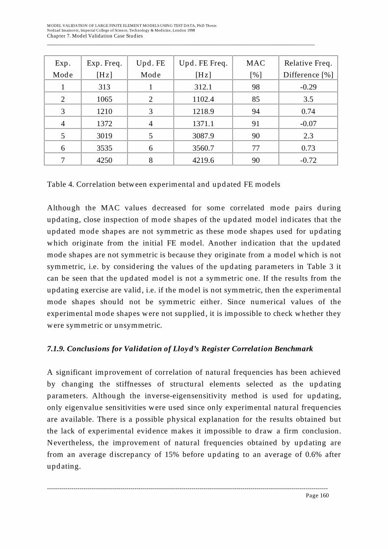
MODEL VALIDATION OF LARGE FINITE ELEMENT MODELS USING TEST DATA, PhD ThesisNedzad Imamovic, Imperial College of Science, Technology & Medicine, London 1998
Chapter 7. Model Validation Case Studies__________________________________________________________________________________________
------------------------------------------------------------------------------------------------------------------------------------------Page 160
Exp.Mode
Exp. Freq.[Hz]
Upd. FEMode
Upd. FE Freq.[Hz]
MAC[%]
Relative Freq.Difference [%]
1 313 1 312.1 98 -0.29
2 1065 2 1102.4 85 3.5
3 1210 3 1218.9 94 0.74
4 1372 4 1371.1 91 -0.07
5 3019 5 3087.9 90 2.3
6 3535 6 3560.7 77 0.73
7 4250 8 4219.6 90 -0.72
Table 4. Correlation between experimental and updated FE models
Although the MAC values decreased for some correlated mode pairs duringupdating, close inspection of mode shapes of the updated model indicates that theupdated mode shapes are not symmetric as these mode shapes used for updatingwhich originate from the initial FE model. Another indication that the updatedmode shapes are not symmetric is because they originate from a model which is notsymmetric, i.e. by considering the values of the updating parameters in Table 3 itcan be seen that the updated model is not a symmetric one. If the results from theupdating exercise are valid, i.e. if the model is not symmetric, then the experimentalmode shapes should not be symmetric either. Since numerical values of theexperimental mode shapes were not supplied, it is impossible to check whether theywere symmetric or unsymmetric.
7.1.9. Conclusions for Validation of Lloyd’s Register Correlation Benchmark
A significant improvement of correlation of natural frequencies has been achievedby changing the stiffnesses of structural elements selected as the updatingparameters. Although the inverse-eigensensitivity method is used for updating,only eigenvalue sensitivities were used since only experimental natural frequenciesare available. There is a possible physical explanation for the results obtained butthe lack of experimental evidence makes it impossible to draw a firm conclusion.Nevertheless, the improvement of natural frequencies obtained by updating arefrom an average discrepancy of 15% before updating to an average of 0.6% afterupdating.

MODEL VALIDATION OF LARGE FINITE ELEMENT MODELS USING TEST DATA, PhD ThesisNedzad Imamovic, Imperial College of Science, Technology & Medicine, London 1998
Chapter 7. Model Validation Case Studies__________________________________________________________________________________________
------------------------------------------------------------------------------------------------------------------------------------------Page 161
7.2. Model Validation of an Aerospace Structure (C-Duct)
7.2.1. Introduction
This second case study is the validation of a FE model of an aerospace structure,known as C-Duct in aerospace industry. Two C-Duct structures hold an aircraftengine between them when the engine is mounted onto the wing of the aircraft. Thestructure itself consists of many one-piece components which are assembled byseveral thousand rivets. The structure is shown in Figure 7-4. The overall measuredmass of the structure is about 435 kg. It is necessary to validate an FE model of thestructure to within 5 percent of natural frequency difference between the test and FEdata.
7.2.2. FE model
The structure is modelled using shell and beam elements and concentrated massesand the final mesh has about 92,000 DOFs. The FE model is shown in Figure 7-5.Estimated mass of the FE model is 430 kg. The list of the initial FE model estimatednatural frequencies is given in Table 5.
7.2.3. Modal Test Data
A free-free modal test was carried out in the range between 0 and 100 Hz. Thestructure was tested for non-linearity by exciting it using different force levels. Itwas found that the dynamic behaviour of the structure is linear within the 0 - 40 Hzfrequency range, but not-linear for the higher frequencies. The list of measurednatural frequencies is given in Table 5. The total number of measured FRFs is 90,and the measurement locations are shown in Figure 7-6.
It is important to stress here that planning of the modal test could not be performedbecause the initial FE model was not available at the time when the modal test wascarried out. This particular validation exercise was done as part of a commercialproject involving major engineering companies and as it is not unusual in thesecircumstances that such delays that can change the course of a validation exercise.However, several checks on modal test data have been done when the initial modelwas made available and it was concluded that a sufficient number of points hasbeen measured.

MODEL VALIDATION OF LARGE FINITE ELEMENT MODELS USING TEST DATA, PhD ThesisNedzad Imamovic, Imperial College of Science, Technology & Medicine, London 1998
Chapter 7. Model Validation Case Studies__________________________________________________________________________________________
------------------------------------------------------------------------------------------------------------------------------------------Page 162
Figure 7-4. C-Duct structure during modal testing.

MODEL VALIDATION OF LARGE FINITE ELEMENT MODELS USING TEST DATA, PhD ThesisNedzad Imamovic, Imperial College of Science, Technology & Medicine, London 1998
Chapter 7. Model Validation Case Studies__________________________________________________________________________________________
------------------------------------------------------------------------------------------------------------------------------------------Page 163
Figure 7-5. FE model of C-Duct structure.
Figure 7-6. Experimental mesh of C-Duct structure.

MODEL VALIDATION OF LARGE FINITE ELEMENT MODELS USING TEST DATA, PhD ThesisNedzad Imamovic, Imperial College of Science, Technology & Medicine, London 1998
Chapter 7. Model Validation Case Studies__________________________________________________________________________________________
------------------------------------------------------------------------------------------------------------------------------------------Page 164
7.2.4. Correlation between measured and the initial FE data sets
The following table gives details of the correlation between the initial FE modelfrequencies and the measured natural frequencies for the C-Duct structure.
ModeNo.
ExperimentalFrequency [Hz]
FE Frequency[Hz]
f FEf exp .
1 9.3 10.5 1.12
2 14.6 17.10 1.14
3 16.1 18.35 1.09
4 17.0 20.26 1.13
5 21.5 26.56 1.21
6 26.9 34.02 1.26
7 30.3 38.82 1.36
8 41.2 43.36 1.05
9 46.9 48.02 1.02
10 60.8 59.02 0.97
11 61.9 71.67 1.25
12 75.2 89.66 1.19
13 75.9 93.52 1.23
14 82.4 99.13 1.20
15 85.2 103.41 1.21
16 97.9 108.25 1.11
Table 5. List of experimental and the initial FE natural frequencies.
Correlation between the experimental and FE mode shapes is given in Figure 7-7.
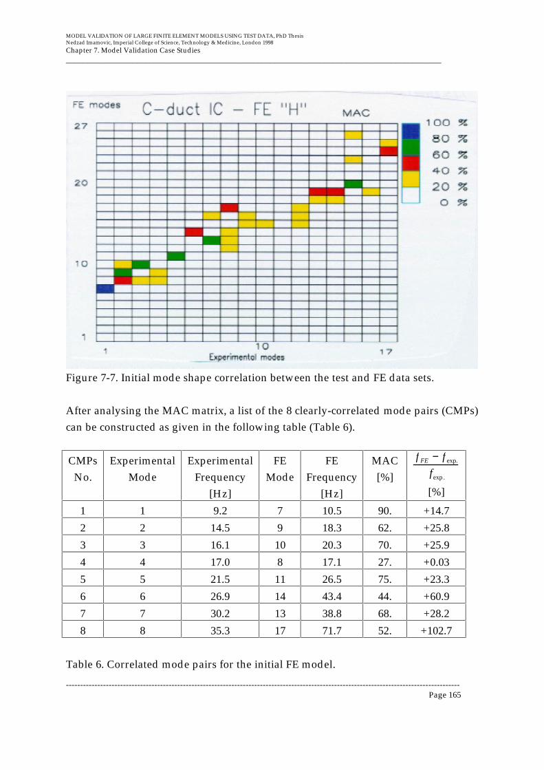
MODEL VALIDATION OF LARGE FINITE ELEMENT MODELS USING TEST DATA, PhD ThesisNedzad Imamovic, Imperial College of Science, Technology & Medicine, London 1998
Chapter 7. Model Validation Case Studies__________________________________________________________________________________________
------------------------------------------------------------------------------------------------------------------------------------------Page 165
Figure 7-7. Initial mode shape correlation between the test and FE data sets.
After analysing the MAC matrix, a list of the 8 clearly-correlated mode pairs (CMPs)can be constructed as given in the following table (Table 6).
CMPsNo.
ExperimentalMode
ExperimentalFrequency
[Hz]
FEMode
FEFrequency
[Hz]
MAC[%]
f FE − f exp.
fexp .
[%]
1 1 9.2 7 10.5 90. +14.7
2 2 14.5 9 18.3 62. +25.8
3 3 16.1 10 20.3 70. +25.9
4 4 17.0 8 17.1 27. +0.03
5 5 21.5 11 26.5 75. +23.3
6 6 26.9 14 43.4 44. +60.9
7 7 30.2 13 38.8 68. +28.2
8 8 35.3 17 71.7 52. +102.7
Table 6. Correlated mode pairs for the initial FE model.

MODEL VALIDATION OF LARGE FINITE ELEMENT MODELS USING TEST DATA, PhD ThesisNedzad Imamovic, Imperial College of Science, Technology & Medicine, London 1998
Chapter 7. Model Validation Case Studies__________________________________________________________________________________________
------------------------------------------------------------------------------------------------------------------------------------------Page 166
7.2.5. Error Localisation
The C-Duct finite element model can be classified as a large model, and has far morepossible updating parameters than the amount of experimental data available. Sinceonly eigenvalue sensitivities are used in updating equation, this means that thenumber of updating parameters must be limited to the number of experimentalnatural frequencies, which is eight in this case. By inspecting the structure, it can beconcluded there are several regions which are relatively crude structural joints.Since each of these regions has quite complicated but uniform structural joints, thismeans that each type of structural joint can be represented by one updatingparameter. It is also important to select regions of the model which have significantstrain energy for the mode shapes which are to be used in updating, and the finalselection of updating parameters is shown in Figure 7-8. Each updating parametercomprises a number of individual finite elements.
Figure 7-8. Selection of updating parameters for C-Duct FE model.

MODEL VALIDATION OF LARGE FINITE ELEMENT MODELS USING TEST DATA, PhD ThesisNedzad Imamovic, Imperial College of Science, Technology & Medicine, London 1998
Chapter 7. Model Validation Case Studies__________________________________________________________________________________________
------------------------------------------------------------------------------------------------------------------------------------------Page 167
It was thought that the mass representation of the structure was properly defined bythe initial FE model and therefore only stiffness correction is to be performed duringupdating. By considering the approximation of the initial FE model it was decidedthat a limit for possible perturbations (or values of the updating parameters) shouldbe set to 60 percent of the initial stiffness value. This effectively meant that there wasa limit on all updating parameters to vary only in the region [-0.6,0.6].
7.2.6. Model Updating
Model updating of the C-Duct structure was performed using the standard inverseeigensensitivity method but using only eigenvalue sensitivities. Eigenvectorsensitivities were not used in updating equation due to the fact that theircontribution to the rank of the sensitivity matrix is negligible and the computationaleffort necessary to calculate them is unreasonably expensive (see chapter 6).
7.2.7. Convergence of updating parameters
Several different initial selection of updating parameters were used during updatingof the C-Duct case study. Identification of the column space of the stiffness matrixwas used during updating in order to stabilise the search process and to ensureconvergence or at least limit divergence. Only about 30 percent of all updatingattempts converged to improved models. A few updating attempts were made forevery single selection of updating parameters with different initial values given tothe updating parameters. Successful iterative search attempts found severaldifferent updated models, one updated model for each iteration. Some of theseupdated models from the same iteration sequence are almost equivalent, but due tothe nature of the searching algorithm there are usually quite a few different updatedmodels for every iteration sequence. At the end, more that 300 updated models werefound and it was necessary to establish some systematic selection process in order todetermine the final updated model.
7.2.8. Selection of the final updated model
When selecting the final updated model several important factors were considered,but particular emphasis was paid to: (i) natural frequency difference of CMPs, (ii)MAC values of CMPs, (iii) values of updating parameters, (iv) global uniqueness of
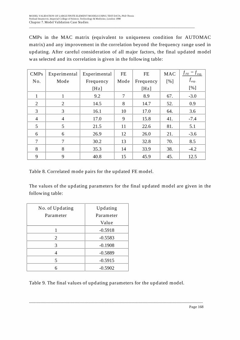
MODEL VALIDATION OF LARGE FINITE ELEMENT MODELS USING TEST DATA, PhD ThesisNedzad Imamovic, Imperial College of Science, Technology & Medicine, London 1998
Chapter 7. Model Validation Case Studies__________________________________________________________________________________________
------------------------------------------------------------------------------------------------------------------------------------------Page 168
CMPs in the MAC matrix (equivalent to uniqueness condition for AUTOMACmatrix) and any improvement in the correlation beyond the frequency range used inupdating. After careful consideration of all major factors, the final updated modelwas selected and its correlation is given in the following table:
CMPsNo.
ExperimentalMode
ExperimentalFrequency
[Hz]
FEMode
FEFrequency
[Hz]
MAC[%]
f FE − f exp.
fexp .
[%]
1 1 9.2 7 8.9 67. -3.0
2 2 14.5 8 14.7 52. 0.9
3 3 16.1 10 17.0 64. 3.6
4 4 17.0 9 15.8 41. -7.4
5 5 21.5 11 22.6 81. 5.1
6 6 26.9 12 26.0 21. -3.6
7 7 30.2 13 32.8 70. 8.5
8 8 35.3 14 33.9 38. -4.2
9 9 40.8 15 45.9 45. 12.5
Table 8. Correlated mode pairs for the updated FE model.
The values of the updating parameters for the final updated model are given in thefollowing table:
No. of UpdatingParameter
UpdatingParameter
Value
1 -0.5918
2 -0.5583
3 -0.1908
4 -0.5889
5 -0.5915
6 -0.5902
Table 9. The final values of updating parameters for the updated model.
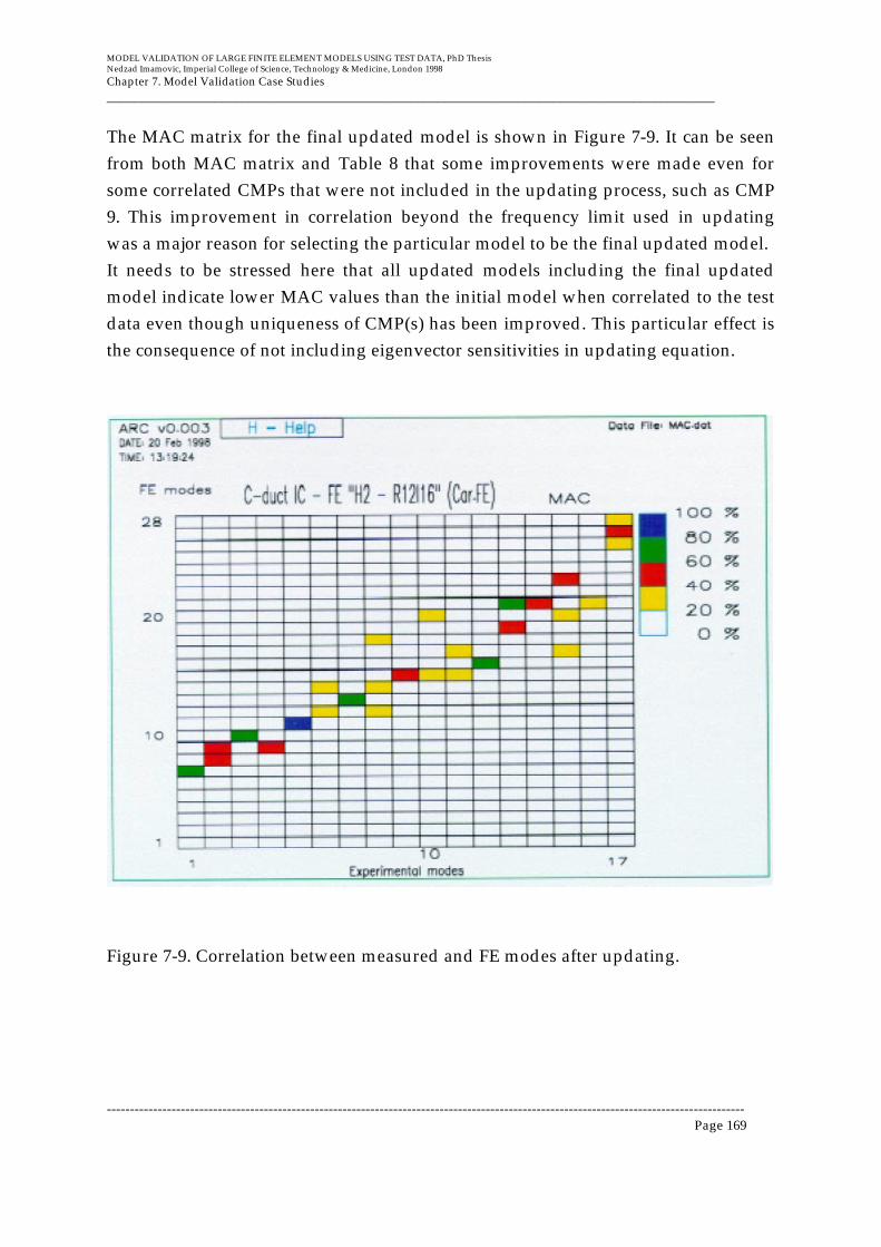
MODEL VALIDATION OF LARGE FINITE ELEMENT MODELS USING TEST DATA, PhD ThesisNedzad Imamovic, Imperial College of Science, Technology & Medicine, London 1998
Chapter 7. Model Validation Case Studies__________________________________________________________________________________________
------------------------------------------------------------------------------------------------------------------------------------------Page 169
The MAC matrix for the final updated model is shown in Figure 7-9. It can be seenfrom both MAC matrix and Table 8 that some improvements were made even forsome correlated CMPs that were not included in the updating process, such as CMP9. This improvement in correlation beyond the frequency limit used in updatingwas a major reason for selecting the particular model to be the final updated model.It needs to be stressed here that all updated models including the final updatedmodel indicate lower MAC values than the initial model when correlated to the testdata even though uniqueness of CMP(s) has been improved. This particular effect isthe consequence of not including eigenvector sensitivities in updating equation.
Figure 7-9. Correlation between measured and FE modes after updating.

MODEL VALIDATION OF LARGE FINITE ELEMENT MODELS USING TEST DATA, PhD ThesisNedzad Imamovic, Imperial College of Science, Technology & Medicine, London 1998
Chapter 7. Model Validation Case Studies__________________________________________________________________________________________
------------------------------------------------------------------------------------------------------------------------------------------Page 170
7.2.9. Conclusions for Validation of C-Duct Structural Dynamic Model
Model validation of the initial structural dynamic model of C-Duct structure wasperformed. The objective of the exercise was to validate natural frequencies within 5percent but this objective was difficult to achieve due to limits imposed onvariations of the updating parameters. However, some mode shapes had higherimportance and these mode shapes satisfied the initial criterion for frequencycorrelation. Eigenvector sensitivities were not used in the updating process due tothe disproportionate calculation effort required to calculate them in respect of theircontribution to the overall conditioning of the sensitivity matrix. After applyingmodel validation to the C-Duct case study more than 300 improved models weregenerated, most of them showing close correlation to the experimental results eventhough every single improved model was different to the others. The selectionprocess proved to be almost as difficult as any other part of model validation andtherefore some additional criteria had to be employed to select one final improvedmodel. The final updated model shows correlation even beyond frequency forwhich model validation was performed.
MODEL VALIDATION OF LARGE FINITE ELEMENT MODELS USING TEST DATA, PhD ThesisNedzad Imamovic, Imperial College of Science, Technology & Medicine, London 1998
Chapter 8. Conclusions and Suggestions for Future Work__________________________________________________________________________________________
------------------------------------------------------------------------------------------------------------------------------------------Page 171
8.0 Conclusions and Suggestions for Future Work
This chapter presents the main conclusions and a summary of the specificcontributions reported in this thesis. The Conclusions section below represents theoverall conclusions for the use of model validation as presented in this thesis whilemore specific conclusions are given at the end of each chapter.
8.1. Conclusions
The main goal of the research reported in this thesis was to study the applicability ofmodel validation to real engineering problems. Since the majority of realengineering problems involve quite complicated structures, see Figure 8.1-1 forexample, these models are usually large in terms of their number of DOFs, andtherefore a particular emphasis was given to applicability of model validation to‘large’ theoretical models.
Before model validation of any structure is attempted, there should always existwell-defined criteria for the validated model. In practice, these criteria are usuallygiven in terms of natural frequency and mode shape differences for a specifiednumber of modes or over a specified frequency range. Validation criteria can befound from the final use of a validated model, i.e. if the validated model is to beused for prediction of general transient response then it is possible to define afrequency region within which the initial model needs to be validated (section2.2.3).
Once validation criteria are found, then it is necessary to determine the minimumdata requirements for validation. Data requirements have been defined separatelyfor correlation and for model updating. In the case of correlation, it has been shownthat it is possible to define the minimum data requirements (section 4.4), while inthe case of model updating it was shown that defining data requirements is not sostraightforward (section 5.1.1).

MODEL VALIDATION OF LARGE FINITE ELEMENT MODELS USING TEST DATA, PhD ThesisNedzad Imamovic, Imperial College of Science, Technology & Medicine, London 1998
Chapter 8. Conclusions and Suggestions for Future Work__________________________________________________________________________________________
------------------------------------------------------------------------------------------------------------------------------------------Page 172
Figure 8.1-1. A typical structure which needs to be modelled accurately.
MODEL VALIDATION OF LARGE FINITE ELEMENT MODELS USING TEST DATA, PhD ThesisNedzad Imamovic, Imperial College of Science, Technology & Medicine, London 1998
Chapter 8. Conclusions and Suggestions for Future Work__________________________________________________________________________________________
------------------------------------------------------------------------------------------------------------------------------------------Page 173
Data requirements for correlation were coupled with test planning to ensure that thenecessary experiments can be optimised. Modal tests on complicated structures canbe quite time-consuming and expensive. It is necessary to ensure that these tests arecarried out with the minimum of effort while the measured data acquired are of thehighest accuracy. During a modal test, it is necessary to select optimum suspension,optimum excitation location(s) and optimum measurement locations, as shown inChapter 3.
Obviously, the test is a critical stage of the model validation process. The test shouldbe carried out according to a test plan and the data requirements for correlation, butsince the initial model used in test planning is of limited accuracy (that is the mainreason for doing validation of the model), it is necessary to spend some timeinvestigating the results produced by the test planning phase to make sure that thefinal modal test does not miss any important data.
Correlation is not just a simple comparison between experimental and theoreticalmodels. Correlation is also used to determine the completeness of the measured dataset. Although correlation is not as complicated as test planning or model updating,performing correlation automatically during updating is quite a complicatedprocess. The main task of correlation is to produce a list of correlated mode pairsand this is critical information for the generation of the sensitivity matrix. Also,during the correlation process a picture of possible error locations can be drawn.Provided that the measured data set is complete, then all discrepancies due to errorssomewhere in the model can be shown and identified during correlation process.
Accurate selection of the sites of the errors responsible for discrepancies shown inthe correlation is a crucial requirement for a successful model validation. There aretwo main approaches for selection of error locations and defining model updatingparameters. One approach is to select error locations according to knowledge aboutthe initial model and likely approximations of the initial model. The secondapproach is to select error locations according to the strain energy distributions forthe modes of interest.

MODEL VALIDATION OF LARGE FINITE ELEMENT MODELS USING TEST DATA, PhD ThesisNedzad Imamovic, Imperial College of Science, Technology & Medicine, London 1998
Chapter 8. Conclusions and Suggestions for Future Work__________________________________________________________________________________________
------------------------------------------------------------------------------------------------------------------------------------------Page 174
Once the updating parameters are selected and defined and the initial correlation isknown, then model validation enters a stage where the initial model is correctedand the final updated model is produced. There are many model updatingtechniques, but very few of them can be applied to real engineering problemssuccessfully. The inverse eigensensitivity method was identified as one of the mostpromising for updating of large theoretical models and this method has beenresearched in-depth from a numerical stability and accuracy point of view. It isrecommended to perform updating using well-conditioned over-determinedupdating equation through a special selection of updating parameters, as explainedin section 6.4.2.
Use of eigenvector sensitivities has been discussed in particular detail and it wasshown that the eigenvector sensitivities’ contribution to the sensitivity matrix rankand conditioning is negligible in comparison with that of the eigenvaluesensitivities. This led to the conclusion that eigenvector sensitivities should not beused in updating, unless a special physically-unjustified weighting is introduced,not least because it is very expensive to calculate them. As only updating usingover-determined equations is recommended, that means that the number ofupdating parameters should not exceed number of CMP(s) determined duringcorrelation.
After several updating attempts are made, it is necessary to select the final updatedmodel. Since model updating does not produce a unique solution, it is commonpractice to find several different updated models giving similar levels of correlationwith the experimental model. The final updated model must be selected byconsideration of some additional criteria which were not used in updating, such ascorrelation of FRFs for the higher frequencies etc.

MODEL VALIDATION OF LARGE FINITE ELEMENT MODELS USING TEST DATA, PhD ThesisNedzad Imamovic, Imperial College of Science, Technology & Medicine, London 1998
Chapter 8. Conclusions and Suggestions for Future Work__________________________________________________________________________________________
------------------------------------------------------------------------------------------------------------------------------------------Page 175
8.2. List of Contributions to Model Validation
8.2.1. Contributions to Test Planning
In test planning, the following contributions have been made and are presented inthis thesis:
(i) new methods for defining the average displacement, velocity and acceleration ofan excited system, ADDOFD, ADDOFV and ADDOFA, respectively;
(ii) a new method for finding the optimum suspension locations based on theADDOFD parameter;
(iii) new methods for analysing the distribution of the nodal lines of an excitedsystem; Optimum Driving Point (ODP) and Non-Optimum Driving Point (NODP)parameters;
(iv) a new method for finding the optimum excitation locations; the ODP method,and guidance on how to use it;
(v) a new method for finding the non-optimum excitation locations; NODP methodand guidance on how to use it;
(vi) a series of new coefficients based on ADDOFV, ADDOFA, ODP and NODPparameters for selection of the optimum excitation location; ODP-V, ODP-A, NODP-V and NODP-A and guidance on how to use them;
(vii) the existing Effective Independence (EI) method was used as the basis fordevelopment of new method for finding the optimum set of measurement locations.New methods use EI and the ADDOFV or ADDOFA parameters to select the bestoptimum locations to measure mode shapes as independently as possible butmeasuring only locations where the highest signal-to-noise ratio is to be found;
(viii) Whether a modal test is to be carried out using a hammer or a shaker forexcitation, and whether the response is to be measured using accelerometers or a

MODEL VALIDATION OF LARGE FINITE ELEMENT MODELS USING TEST DATA, PhD ThesisNedzad Imamovic, Imperial College of Science, Technology & Medicine, London 1998
Chapter 8. Conclusions and Suggestions for Future Work__________________________________________________________________________________________
------------------------------------------------------------------------------------------------------------------------------------------Page 176
laser velocimeter, a complete test planning strategy is developed and presented inthis thesis;
(ix) all new methods were verified on many practical test cases, a few of which areincluded in this thesis.
8.2.2. Contributions to Correlation
In correlation, the following new methods and contributions have been made:
(i) a relatively new method for assessment of complexity of experimental modeshapes has been defined and explained in detail and a discussion about realisationof complex mode shapes is given;
(ii) a new correlation coefficient, the SEREP Cross-Orthogonality (SCO), based onthe SEREP reduction process, is introduced with all the required and sufficientconditions for its successful use clearly defined;
(iii) a new coefficient for comparison of natural frequencies, Natural FrequencyDifference (NFD), has been defined;
(iv) a new correlation procedure for selection of correlated mode pairs is presented.This correlation procedure is used in model updating approach as a tool forautomatic selection of CMPs;
(v) a new method for determination of the necessary number of out-of-range modesfor calculation of FRFs with controlled accuracy of antiresonances has beendeveloped and presented, abbreviated as the FOREST technique.
8.2.3. Contributions to Error Location Methods
The following contributions to error location methods have been made:
(i) a detailed explanation of problems associated with solving model updating as anidentification problem;

MODEL VALIDATION OF LARGE FINITE ELEMENT MODELS USING TEST DATA, PhD ThesisNedzad Imamovic, Imperial College of Science, Technology & Medicine, London 1998
Chapter 8. Conclusions and Suggestions for Future Work__________________________________________________________________________________________
------------------------------------------------------------------------------------------------------------------------------------------Page 177
(ii) new limitations for updating parameter values have been presented andexplained;
(iii) two different approaches for selection of model updating parameters have beenintroduced, empirically- and sensitivity-based selection methods;
(iv) a comprehensive study of distribution of error locations to the overall objectivefunction based on random error distribution theory.
8.2.4. Contributions to Model Updating
In model updating the following contributions have been made:
(i) a new definition of the updated model is given;
(ii) a systematic selection of existing promising updating approaches to be used forvalidation of large finite element models;
(iii) a comprehensive study of all possible scenarios for solving the least-squaresproblem when applied in model updating using the Inverse Eigensensitivitymethod;
(iv) a new method for elimination of ill-conditioning of the sensitivity matrix andselection of updating parameters based on finding the best column space of thematrix;
(v) use and contribution of mode shape sensitivities for updating of large finiteelement models has been discussed.
8.3. Suggestions for Future Work
Model validation is reaching a stage at which it is becoming more and more activelyused within industry, particularly for aerospace applications. Today, there are moreand more situations within industrial practice when a company asks its supplier toprovide a validated model of an ordered product. These products vary from simplecomponents to aircraft engines or planes. One can almost certainly expect that the
MODEL VALIDATION OF LARGE FINITE ELEMENT MODELS USING TEST DATA, PhD ThesisNedzad Imamovic, Imperial College of Science, Technology & Medicine, London 1998
Chapter 8. Conclusions and Suggestions for Future Work__________________________________________________________________________________________
------------------------------------------------------------------------------------------------------------------------------------------Page 178
need for model validation will increase in the future and therefore furtherdevelopments are ensured, the only uncertainty being the way in which thistechnology will be developed. The latest developments suggest that there is anincreasing trend towards the use of model validation for damage detection. Thisseems as an obvious and natural path that model validation application will follow.Also, further integration between experimental methods and theoretical predictionsis expected, not only within the structural dynamics field, but further, combiningfluid-dynamic effects with structural dynamics.
There are some encouraging findings and results presented in this thesis, but thereare also some results (see section 5.2.1, Figure 5.2.1-2) which indicate that there isstill some way to go before model validation can be used as a routine tool forindustrial applications. Further development of model validation technology isnecessary to bring it to a stage where every engineer with the minimum of specialistknowledge about model validation techniques can safely use this technology as ablack-box routine. In order to ensure that further development of this technologybrings it a step closer to wide industrial application the following areas need to beresearched.
(i) Integration of final use of the validated model and validation techniques, test
planning, correlation and updating. Every validation exercise is attempted with aspecific goal - usually, this goal is to match particular modes for given the frequencytolerance - and this information must be used as the initial data for determining theminimum data requirements for correlation and updating. If the final user of thevalidated model knows what the validated model is intended for, then thisknowledge should be converted into numerical form which can indicate thefrequency range of validation and the required level of correlation in this frequencyrange. In practice, if a company requires model validation to be performed for aspecific purpose, then the party who undertakes the validation task should be ableto define the required level of correlation and the frequency range of validation.Nowadays, everyone wants their models to be validated within a specific frequencyrange but little or nothing is known about the reliability of these validated modelswhen used for further analysis.

MODEL VALIDATION OF LARGE FINITE ELEMENT MODELS USING TEST DATA, PhD ThesisNedzad Imamovic, Imperial College of Science, Technology & Medicine, London 1998
Chapter 8. Conclusions and Suggestions for Future Work__________________________________________________________________________________________
------------------------------------------------------------------------------------------------------------------------------------------Page 179
(ii) Error location theory needs to be further developed and better understood
than it is the case today. Every validation exercise should be used to explaindiscrepancies so that model validation is also used as a tool for learning aboutimproved modelling. As more sophisticated and perhaps new modelling techniquesdeveloped through model validation are used, the boundary of the expectedvalidation level will move further. Today, it is standard practice not to expect morethan 20 (certainly 30) modes in general to have an acceptable correlation. Thisboundary will move as model validation techniques improve, new modellingtechniques are used and, obviously, as new measurement techniques are madeavailable. It is important to understand physical changes made to the initial modelwhenever possible rather than just to take changes to the initial model blindlywithout properly understanding errors of the initial model.
(iii) Determination of data requirements for model updating. It was shown inChapter 5 that it is virtually impossible to gather sufficient data for a completeidentification of the structural model. However, it should be possible to find arelationship between the accuracy of the validated model (for a specific purpose, ofcourse) and the data requirements. It is almost certain that the data requirements formodel updating will be huge, although perhaps not unattainable as in the modelidentification case, but at least by knowing this relationship it will be possible toassess whether the current approaches used in model updating are feasible. Also, itwould be interesting to explore the dependency of different updating formulationson the data requirements for model updating.
(iv) Further study is needed of the validation data requirements of an assembled
structure. Clearly, single components must be validated within a higher frequencyrange than applied to the assembled structure. This approach of disassemblingstructure and validating single components first and then assembling the structureand validating every subassembly is a natural way of validation for complicatedstructures.
(v) Development of new updating algorithms using stochastic optimisation
techniques. The objective function diagrams presented in Chapter 5 clearly showdifficulties associated with model updating. Optimisation of objective functionswhich originate from model updating is extremely difficult to solve. So far noknown search algorithm can even expect to find the global optimum of these

MODEL VALIDATION OF LARGE FINITE ELEMENT MODELS USING TEST DATA, PhD ThesisNedzad Imamovic, Imperial College of Science, Technology & Medicine, London 1998
Chapter 8. Conclusions and Suggestions for Future Work__________________________________________________________________________________________
------------------------------------------------------------------------------------------------------------------------------------------Page 180
functions and therefore some more sophisticated optimisation procedures, such asGenetic Algorithms or Simulated Annealing, need to be explored for this purpose.
8.6. A Final Word
Model validation technology and the current know-how about it have beenpresented in this thesis. Some results are extremely encouraging even though somefindings showed serious problems associated with model validation and itsapplication. Clearly, there is still some way to go before this technology becomesmature for wide-scale application in industry but, in general, it can be said thatapplication of model validation (by specialists) is readily available. Modelvalidation is equally important as a field which drives and highlights the need forfurther development of experimental techniques.
A specific goal in this thesis was to make model validation more applicable as a toolfor validation of models in practice. This has been achieved by a thoroughunderstanding of current developments, by developing new techniques presentedherein, and by applying model validation to many industrial applications.
MODEL VALIDATION OF LARGE FINITE ELEMENT MODELS USING TEST DATA, PhD ThesisNedzad Imamovic, Imperial College of Science, Technology & Medicine, London 1998
Reference__________________________________________________________________________________________
------------------------------------------------------------------------------------------------------------------------------------------Page 181
References
[1] Natke H GUpdating Computational Models in the Frequency Domain Based on Measured Data: A SurveyProbabilistic Engineering Mechanics, Vol. 4, No. 1, 1988
[2] Ewins, D JModal Testing: Theory and PracticeResearch Studies Press Ltd., 1984
[3] T W LimActuator/Sensor Placement for Modal Parameter Identification of Flexible StructuresModal Analysis, 8(3). 1993.
[4] The Dynamic Testing Agency & NAFEMSInternational Conference - Structural Dynamics Modelling, Test, Analysis and CorrelationNAFESM, 1993
[5] R J GuyanReduction of Stiffness and Mass MatricesAIAA Journal 3(2),380, 1965
[6] D C KammerSensor Placement for On-Orbit Modal Identification and Correlation of Large Space StructuresJournal of Guidance, Control and Dynamics, 14(2),251-259, 1991
[7] Allemang, R J and Brown, D LA Correlation Coefficient for Modal Vector AnalysisProc. of the 1st Int. Modal Analysis Conf., pp 110-116, 1982
[8] N A J Lieven and T P WatersError Location using Normalised Orthogonality12th IMAC, Honolulu, Hawaii, 1994
[9] GH Golub, CF Van LoanMatrix ComputationsSecond Edition. The John Hopkins University Press. London 1993.
[10] M I Friswell, J E MottersheadFinite Element Model Updating In Structural Dynamics

MODEL VALIDATION OF LARGE FINITE ELEMENT MODELS USING TEST DATA, PhD ThesisNedzad Imamovic, Imperial College of Science, Technology & Medicine, London 1998
Reference__________________________________________________________________________________________
------------------------------------------------------------------------------------------------------------------------------------------Page 182
Kluwer Academic Publishers. ISBN 0-7923-3431-0. 1995.[11] N A J Lieven, D J Ewins
Spatial Correlation of Mode Shapes, the Coordinate Modal Assurance Criterion (COMAC)6th IMAC, Orlando, Florida, 1988
[12] M Imregun, DJ EwinsAn Investigation into mode shape expansion techniques11th IMAC, Florida 1993
[13] C O’Callahan, P Avitabile, I Lieu, R MAddenAn efficient method of determining rotational degrees of freedom from analytical and experimental modal data4th IMAC, Los Angeles, CA, February 1986
[14] P Avitable, J O’Callahan, J MilaniComparison of system characteristics using various model reduction techniques7th IMAC, Las Vegas, Nevada, February 1989
[15] M PazDynamic CondensationAIAA Journal, 22(5), 724-727, 1984
[16] Sidhu, J, Ewins D JCorrelation of Finite Element and Test Studies of a practical Structure2nd IMAC, 1984
[17] Baruch, MOptimisation procedure to Correct Stiffness and Flexibility Matrices using Vibration TestsAIAA Journal, Vol. 16, No. 11, 1978
[18] Berger H, Chaquin J P, Ohayon RFinite Element Model Adjustment using Experimental Modal Data2dn IMAC, 1984
[19] Link MComparison of Porcedures for Localising and Correcting Errors in Computational Models using Test Data9th IMAC, 1991
[20] Link M, Zhang LExperience with Different Procedures for Updating Structural Parameters ofAnalytical Models using test Data

MODEL VALIDATION OF LARGE FINITE ELEMENT MODELS USING TEST DATA, PhD ThesisNedzad Imamovic, Imperial College of Science, Technology & Medicine, London 1998
Reference__________________________________________________________________________________________
------------------------------------------------------------------------------------------------------------------------------------------Page 183
10th IMAC, 1992[21] Niedbal N, Klusowski E, Luber W
Updating of Finite Element Model by Means of Normal Mode Parameters13th International Seminar on Modal Analysis, K U Leuven, 1988
[22] Collins J D, Hart G C, Hasselman T K, Kennedy BStatistical Identification of StructuresAIAA Journal, Vol. 12, No. 2, 1974
[23] Chen J C, Wada B KCriteria for Analysis - Test Correlation of Structural Dynamic SystemsJournal of Applied Mechanics, 1975
[24] Inman D J, Minas CMatching Analytical Models with Experimental Modal Data in Mechanical SystemsControl and Dynamic Systems, Vol. 37, 1990
[25] Minas C, Inman D JMatching Finite Element Models to Modal DataASME Journal of Vibration and Acoustics, Vol. 112, 1990
[26] R M Lin, D J EwinsModel Updating using FRF Data15th International Modal Analysis Seminar, K U Leuven, Belgium, 141-163, 1990
[27] K J BatheFinite Element Procedures in Engineering AnalysisPrentice Hall, New Jersey, 1982
[28] B M Irons, S AhmadTechniques of Finite ElementsEllis Horwood, Chichester, 1980
[29] MSC/NASTRANHandbook for Numerical MethodsThe MacNeal-Schwendler Corporation, Los Angeles, 1990
[30] NAFEMSA Finite Element PrimerNational Agency for Finite Element Methods and Standards, 1986
[31] O C Zienkiewicz, R L TaylorThe Finite Element Method, Vol. 1
MODEL VALIDATION OF LARGE FINITE ELEMENT MODELS USING TEST DATA, PhD ThesisNedzad Imamovic, Imperial College of Science, Technology & Medicine, London 1998
Reference__________________________________________________________________________________________
------------------------------------------------------------------------------------------------------------------------------------------Page 184
4th Edition, McGraw-Hill, London, 1988[32] D E Newland
An Introduction to Random Vibrations and Spectral Analysis2dn Edition, Longman Group Ltd., 1985
[33] N Imamovic, D J Ewins
Optimization of Excitation DOF Selection for Modal Test15th IMAC, 1997.
[34] N Imamovic
preliminary FE Analysis Results of the Lloyd’s Register Correlation Benchmark (Ref.: CIV/9334/jrm)Imperial College Technical Notes. 1995.
[35] M Imregun and DJ EwinsComplex Modes - Origins and Limits13th IMAC, Nashville, Tennessee, 1995
[36] S R IbrahimComputation of Normal Modes from Identified Complex ModesAIAA Journal, 21(3), 446-451
[37] N Imamovic, D J Ewins
An Automatic Correlation Procedure for Structural DynamicsCEAS Conference 1995 in Manchester, England.
[38] T Soderstrom, P StoicaSystem IdentificationPrentice Hall Informational Series in Systems and Control Engineering, London, 1989
[39] J D Collins, G C Hart, T K Hasselman, B KennedyStatistical Identification of StructuresAIAA Journal, 12(2), 185-190, 1974
[40] A Berman, W G FlannelyTheory of Incomplete Models of Dynamic StructuresAIAA Journal, 9(8), 1481-1487, 1971
[41] Mottershead J E, Friswell M IFinite Element Model Updating in Structural DynamicsKluwer Academic Publishers. ISBN 0-7923-3431-0, 1995.

MODEL VALIDATION OF LARGE FINITE ELEMENT MODELS USING TEST DATA, PhD ThesisNedzad Imamovic, Imperial College of Science, Technology & Medicine, London 1998
Reference__________________________________________________________________________________________
------------------------------------------------------------------------------------------------------------------------------------------Page 185
[42] O C Zienkiewicz, J Z ZhuA Simple Error Estimator and Adaptive Procedure for PracticalEngineering AnalysisInternational Journal of Numerical Methods in Engineering, 24, 337-357, 1987
[43] A BermanLimitations on the identification of discrete structural dynamic models2nd International Conference on Recent Advances in Structural Dynamics, Southampton, 427-435, 1984
[44] M I FriswellCandidate Reduced Order Models for Structural Parameter EstimationTransaction of the ASME, Journal of Vibration and Acoustics, 112(1), 93-97, 1990
[45] M link, O F SantiagoUpdating and Localizing Structural Errors Based on Minimisation of Equation ErrorsInternational Conference on Spacecraft Structures and Mechanical Testing, ESA/ESTEC, Noordwijk, Holland, 1991
[46] R Horst, P M PardalosHandbook of Global OptimizationKluwer Academic Publishers, 1995The Netherlands
[47] Mottershead J E, Friswell M IModel Updating in Structural Dynamics: A SurveyJournal of Sound and Vibration, 167(2), 1993.
[48] S Chatterjee, A S HadiSensitivity Analysis in Linear RegressionJohn Wiley & Sons, Inc., 1988
[49] T L Boullion, P L OdellGeneralised Inverse MatricesWiley-Interscience 1971 USA
[50] R B NelsonSimplified Calculation of Eigenvector DerivativesAIAA Journal, 14(9), 1201-1205, 1976

MODEL VALIDATION OF LARGE FINITE ELEMENT MODELS USING TEST DATA, PhD ThesisNedzad Imamovic, Imperial College of Science, Technology & Medicine, London 1998
Reference__________________________________________________________________________________________
------------------------------------------------------------------------------------------------------------------------------------------Page 186
[51] R M Pringle and AA RaynerGeneralised Inverse Matrices with applications to statisticsGriffin London 1971
[52] D Kahaner, C Moler, S NashNumerical Methods and SoftwarePrentice-Hall, Inc., 1989
[53] N R Draper, H SmithApplied Regression AnalysisJohn Wiley & Sons, Inc., Second Edition, 1981
[54] J E MottorsheadTheory of the Estimation of Structural Vibration Parameters from Incomplete DataAIAAJournal, 28(7), 1326-1328, 1990
[55] G Golub, V Klema, G W Stewart
Rank Degeneracy and Least Squares ProblemStanford University Publication, STAN-CS-76-559, 1976
[56] O’Callahan, P Avitable, R RiemerSystem equivalent reduction expansion process(SEREP)7th IMAC, Las Vegas, Nevada, February 1989
[57] ICATS Reference ManualICATS, Imperial College of Science & TechnologyExhibition Road, London SW7, 1988
[58] D J EwinsA Survey to Assess the Reliability of Mobility Measurement TechniquesImperial College of Science and Technology, London
[59] W J VisserUpdating Structural Dynamics Models Using Frequency Response DataPhD, Imperial College, London. 1992.
[60] Notation for Modal Testing & AnalysisVersion A1.01, January 1993, Imperial College, London
[61] Bishop, R E D and Johnson, D CThe Mechanics of VibrationCambridge University Press, 1960
MODEL VALIDATION OF LARGE FINITE ELEMENT MODELS USING TEST DATA, PhD ThesisNedzad Imamovic, Imperial College of Science, Technology & Medicine, London 1998
Reference__________________________________________________________________________________________
------------------------------------------------------------------------------------------------------------------------------------------Page 187
[62] JET Penny, MI Friswell, D S GarveyThe Automatic Choice of measurement locations for dynamic testing11th IMAC 30-36, Florida 1993
[63] LMS InternationalLarge-Scale Modal Testing of a Space Frame Structure - from Pretest Analysis to FEA Model ValidationSound And Vibration/Volume 25/No. 3/March 1991
[64] D C KammerEffect of Noise on Sensor Placement for On-orbit Modal Identification and Correlation of Large Space structuresJournal of Dynamical Systems, Measurement and Control - Transactions of
ASME, 114(3), 436-443, 1992
[65] M L M Duarte, D J EwinsHigh-Frequency Pseudo-Mode Approximation for the High-Frequency Residual TermsPaper submitted to IMAC XIV
[66] J A BrandonStrategies for Structural Dynamic ModificationResearch Studies press Ltd., Somerset, England, 1990
[67] I U OjalvoEfficient Computation of Mode-Shape Derivatives for Large Dynamic SystemsAIAA Journal, 25(10), 1386-1390, 1987
[68] T R Sutter, C J Camarda, J L Walsh, H M AdelmansComparison of Several Methods for Calculating Vibration Mode Shape DerivativesAIAA Journal, 26(12), 1506-1511, 1988
[69] J H WilkinsonThe Algebraic Eigenvalue ProblemOxford University Press (Clarendon), London, 1965
[70] S R IbrahimComputation of Normal Modes from Identified Complex ModesAIAAJournal, 21(3), 446-451, 1983

MODEL VALIDATION OF LARGE FINITE ELEMENT MODELS USING TEST DATA, PhD ThesisNedzad Imamovic, Imperial College of Science, Technology & Medicine, London 1998
Reference__________________________________________________________________________________________
------------------------------------------------------------------------------------------------------------------------------------------Page 188
[71] Y Ben-NaimAdaptive Model Updating by Selective Sensitivity: Overview and New ResultsInternational Journal of Numerical Methods in Engineering, To be published.
[72] A BermanSystem Identification of Structural Dynamic Models - Theoretical and Practical BoundsAIAA Conference Paper 84-0929, 1984
[73] S Cogan, G Lallement, Y Ben-HaimUpdating Linear Elastic Models with Modal-Based Selective Sensitivity12th IMAC, Honolulu, Hawaii, 1994
[74] E Fissette, S IbrahimError Location and Updating of Analytical Dynamic Models using a force balance method6th IMAC, Orlando, Florida, 1063-1070, 1988
[75] G Golub, C Van LoanAn Analysis of the Total Least Squares ProblemSIAM Journal of Numerical Analysis, 17, 883-893, 1980
[76] W Gawronski, H G NatkeOn ARMA Models for Vibrating SystemsProbabilistic Engineering Mechanics, 1(3), 150-156, 1986
[77] W Gawronski, H G NatkeOrder Estimation of AR and ARMA ModelsInternational Journal of Systems Science, 19(7), 1143-1148, 1988
[78] G Lallement, J PirandaLocalisation Methods for Parameter Updating of Finite Element Models in Elastodynamics8th IMAC, Orlando, Florida, 579-585
[79] L LjungSystem Identification - Theory for the UserPrentice Hall Information and Systems Sciences Series, Englewood Cliffs, 1987

MODEL VALIDATION OF LARGE FINITE ELEMENT MODELS USING TEST DATA, PhD ThesisNedzad Imamovic, Imperial College of Science, Technology & Medicine, London 1998
Reference__________________________________________________________________________________________
------------------------------------------------------------------------------------------------------------------------------------------Page 189
[80] J E Mottershead, C D FosterOn the Treatment of Ill-Conditioning in Spatial Parameter Estimation from Measured Vibration DataMechanical Systems and Signal Processing, 5(2), 139-154, 1991
[81] J E Mottershead, W ShaoCorrection of Joint Stiffnesses and Constraints for Finite Element Models in
Structural DynamicsTransaction of ASME, Journal of Applied Mechanics, 60(1), 117-122, 1993
[82] J E Mottershead, E L Goh, W ShaoOn the Treatment of Discretisation Errors in Finite Element Model Updating17th International Modal Analysis Seminar, K U Leuven, 1245-1262, 1992
[83] H G NatkeUpdating Computational Models in the Frequency Domain based on Measured Data: A SurveyProbabilistic Engineering Mechanics, 3(1), 28-35, 1988
[84] H G NatkeOn Regularisation Methods Applied to the Error Localisation of Mathematical Models9th IMAC, Florence, Italy, 70-73, 1991
[85] I U Ojalvo, T TingInterpretation and Improved Solution Approach for Ill-ConditionedLinear EquationsAIAA Journal, 28(11), 1976-1979, 1989
[86] I U OjalvoEfficient Solution of Ill-Conditioned Equations Arising in System Identification8th IMAC, Orlando, Florida, 554-558, 1990
[87] H RakeStep Response and Frequency Response MethodsAutomatica, 16, 519-526, 1980
[88] Van Huffel, VandewalleThe Use of Total least Squares Techniques for Identification and Parameter EstimationIFAC Conference on Identification and System Parameter Estimation, York, 1167-1172, 1985

MODEL VALIDATION OF LARGE FINITE ELEMENT MODELS USING TEST DATA, PhD ThesisNedzad Imamovic, Imperial College of Science, Technology & Medicine, London 1998
Reference__________________________________________________________________________________________
------------------------------------------------------------------------------------------------------------------------------------------Page 190
[89] Q Zhang, G LallementDominant Error Localisation in a Finite Element Model of a Mechanical StructureMechanical Systems and Signal Processing, 1(2), 141-149, 1987
[90] A Berman, E J NagyImprovement of a Large Analytical Model using Test DataAIAA Journal, 17(8), 1168-1173, 1983
[91] B CaesarUpdating System Matrices using Modal Test Data5th IMAC, London, England, 453-459, 1987
[92] C Minas, D J InmanCorrecting Finite Element Models with Measured Modal Results using Eigenstracture Assignment methods6th IMAC, , 583-587, 1988
[93] S W Smith, C A BeattieSecant-Method Adjustment for Structural ModelsAIAA Journal, 29(1), 119-126, 1991
[94] F-S WeiStructural Dynamic Model Modification using Vibration Test Data7th IMAC, Las Vegas, Nevada, 562-567, 1989
[95] F-S WeiStructural Dynamic Model Improvement using Vibration Test DataAIAA Journal, 28(1), 175-177, 1990
[96] F-S WeiMass and Stiffness Interaction Effects in Analytical Model ModificationAIAA Journal, 28(9), 1686-1688, 1990
[97] D C Zimmerman, M WidengrenCorrecting Finite Element Models using a Symmetric Eigenstructure Assignment TechniqueAIAA Journal, 28(9), 1670-1676, 1990
[98] K D Blakely, W B WaltonSelection of Measurement and Parameter Uncertainties for Finite Element Model Revision2nd IMAC, , 82-88, 1984

MODEL VALIDATION OF LARGE FINITE ELEMENT MODELS USING TEST DATA, PhD ThesisNedzad Imamovic, Imperial College of Science, Technology & Medicine, London 1998
Reference__________________________________________________________________________________________
------------------------------------------------------------------------------------------------------------------------------------------Page 191
[99] K Chen, D L Brown, V T NicolasPerturbed Boundary Condition Model Updating11th IMAC, Kissimmee, Florida, 661-667, 1993
[100] M I FriswellThe Adjustment of Structural Parameters using a Minimum Variance EstimatorJournal of Mechanical Systems and Signal Processing, 3(2), 143-155, 1989
[101] S Lammens, W Heylen, P Sas, D BrownModel Updating and Perturbed Boundary Condition Testing11th IMAC, Kissimmee, Florida, 449-455, 1993
[102] S Li, H Vold, D L BrownApplication of UMPA to PBC Testing11th IMAC, Kissimmee, Florida, 223-231, 1993
[103] N G Nalitolela, J E T Penny, M I FrisswellUpdating Structural Parameters of a Finite Element Model by Adding Mass or Stiffness to the System8th IMAC, , 836-842, 1990
[104] N G Nalitolela, J E T Penny, M I FrisswellA Mass or Stiffness Addition Technique for Structural Parameter UpdatingInternational Journal of Analytical and Experimental Modal Analysis, 7(3), 157-168, 1992
[105] E Rothwell, B DrachmanA Unified Approach to Solving ill-conditioned Matrix ProblemInternational Journal for Numerical Methods in Engineering, 28, 609-620, 1989
[106] C N Felgenhauer, H G NatkeOn the Parameter Identification of Elastomechanical Systems using Input and Output ResidualsIngenieur Archiv, 54(5), 378-387, 1984
[107] C D Foster, J E MottersheadA Method for Improving Finite Element Models by using Experimental Data: Application and Implication for Vibration MonitoringInternational Journal of Mechanical Sciences, 32(3), 191-203, 1990

MODEL VALIDATION OF LARGE FINITE ELEMENT MODELS USING TEST DATA, PhD ThesisNedzad Imamovic, Imperial College of Science, Technology & Medicine, London 1998
Reference__________________________________________________________________________________________
------------------------------------------------------------------------------------------------------------------------------------------Page 192
[108] M I FriswellUpdating Physical Parameters from Frequency Response, Function Data12th Biennial ASME Conference on Mechanical vibration and Noise, Montreal, Canada, DE-Vol 18-4, 393-400, 1989
[109] M I FriswellCandidate Reduced Order Models for Structural Parameter EstimationTransaction of the ASME, Journal of Vibration and Acoustic, 112(1), 93-97, 1990
[110] M I Friswell, J E T PennyUpdating Model Parameters from Frequency Domain Data via Reduced Order ModelsMechanical Systems and Signal processing, 3(5), 377-391, 1990
[111] M I Friswell, J E T PennyThe Effect of Close or Repeated Eigenvalues on the Updating of Model Parameters from FRF DataTransactions of the ASME, Journal of Vibration and Acoustics, 114(4), 514-520, 1992
[112] C P Fritzen, S ZhuUpdating of Finite Element Models by Means of Measured InformationComputers and Structures, 40(2), 475-486, 1991
[113] L LjungSystem Identification: Theory for the UserPrentice Hall, 1987
[114] J E Mottershead, R StanwayIdentification of Structural Vibration Parameters by using a Frequency Domain FilterJournal of Sound and Vibration, 109(3), 495-506, 1986
[115] J E Mottershead, C D FosterOn the Treatment of Ill-conditioning in Spatial Parameters Estimation from Measured Vibration DataMechanical Systems and Signal Processing, 5(2), 139-154, 1991
[116] J E Mottershead, S WeixunOn the Tuning of Analytical Models by using Experimental Vibration Data4th International Conference on Recent Advances in Structural Dynamics, Southampton, UK, 432-443, 1991
MODEL VALIDATION OF LARGE FINITE ELEMENT MODELS USING TEST DATA, PhD ThesisNedzad Imamovic, Imperial College of Science, Technology & Medicine, London 1998
Reference__________________________________________________________________________________________
------------------------------------------------------------------------------------------------------------------------------------------Page 193
[117] A G Nalecz, J WicherDesign Sensitivity Analysis of Mechanical Systems in Frequency DomainJournal of Sound and Vibration, 120(3), 517-526, 1988
[118] H G NatkeUpdating Computational Modes in the Frequency Domain Based on Measured Data: A SurveyProbabilistic Engineering Mechanics, 3(1), 28-35, 1988
[119] A Sestieri, W D’AmbrogioWhy be Modal: How to Avoid the use of Modes in the Modification of Vibrating SystemsInternational Journal of Analytical and Experimental Modal Analysis, 4(1), 25-30, 1989
[120] R S Sharp, P C BrooksSensitivities of Frequency Response Function of Linear Dynamic systems to
Variations in Design Parameter ValuesJournal of Sound and Vibration, 126(1),167-172, 1988
[121] S S SimonianInverse Problems in Structural Dynamics - I. TheoryInternational Journal of Numerical Methods in Engineering, 17(3), 357-365, 1981
[122] S S SimonianInverse Problems in Structural Dynamics - I. ApplicationsInternational Journal of Numerical Methods in Engineering, 17(3), 367-386, 1981
[123] M Brughmans, J Leuridan, K BlauwkampThe Application of FEM-EMA Correlation and Validation Technique on a Body-in-White11th IMAC, Kissimmee, Florida, 646-654, 1993
[124] M Brughmans, F LembregtsUsing Experimental Normal Modes for Analytical Model Updating8th IMAC, Kissimmee, Florida, 389-396, 1993
[125] F Lembregts, M BrughmansEstimation of Real Modes From FRF’s via Direct Parameter Identification7th IMAC, Las Vegas, Nevada, 631-636, 1989

MODEL VALIDATION OF LARGE FINITE ELEMENT MODELS USING TEST DATA, PhD ThesisNedzad Imamovic, Imperial College of Science, Technology & Medicine, London 1998
Reference__________________________________________________________________________________________
------------------------------------------------------------------------------------------------------------------------------------------Page 194
[126] H Zeischka, O Storrer, J Leuridan, U VandeurzenCalculation of Modal Parameter Sensitivity based on a FEM Proportionality
Assumption6th IMAC, Orlando, Florida, 1988
[127] Y K Cheung, M F YeoA Practical Introduction to Finite Element AnalysisPitman Publishing Ltd., 1979
[128] N Imamovic
Correlation of a Structural Dynamics Model of RB211 524 H3 HP RotorRolls-Royce Report No. VUTC/E2/94004
[129] N Imamovic
Notes on the interface between different FE packages in the Centre of Vibration EngineeringRolls-Royce Tec. Notes No. E2001/NI/060694
[130] N Imamovic
Interface Programs for SJ30 Correlation Program - Users’ GuideRolls-Royce Tec. Notes No. E2001/NI/240495
[131] N Imamovic
An Automatic Correlation Procedure for Structural DynamicsRolls-Royce Report No. VUTC/E2/95006
[132] N Imamovic
Methods for Selection of Measurement Points for Modal Testing - Average Driving Point Residue (ADPR) MethodRolls-Royce Report No. VUTC/E2/95007
[133] N Imamovic
A Method to Determine the Residual Effects for FRF CalculationsRolls-Royce Report No. VUTC/E2/95009.

MODEL VALIDATION OF LARGE FINITE ELEMENT MODELS USING TEST DATA, PhD ThesisNedzad Imamovic, Imperial College of Science, Technology & Medicine, London 1998
Reference__________________________________________________________________________________________
------------------------------------------------------------------------------------------------------------------------------------------Page 195
[134] N Imamovic
Application of Model Correlation Methods to SAMM II B Structural Dynamic AnalysisRolls-Royce Report No. VUTC/E2/95011.
[135] N Imamovic
Application of Model Correlation Methods to ISOGRID Fan Case Dynamic AnalysisRolls-Royce Report No. VUTC/E2/95012.
[136] G Chen, N Imamovic
Modal test and Analysis of the Nozzle Substructure (Pegasus Project)Rolls-Royce Report No. VUTC/E2/96012.
[137] N Imamovic
Determination of Optimal Excitation Positions for Modal testing - The ODP and NODP TechniquesRolls-Royce Report No. VUTC/E2/96004.
[138] N Imamovic
Methods for Selection of Measurement DOF for Modal Testing - Effective Independence (EI) Method and ADPR-EI MethodRolls-Royce Report No. VUTC/E2/96002.
[139] N Imamovic
Model Validation of Lloyd;s Register Structural Dynamics Correlation Benchmark (Ref.: CIV/9334/jrm)Rolls-Royce Report No. VUTC/E2/96003.
[140] G Chen
Summary Report on Pegasus Carcase Model Validation ProjectRolls-Royce Report No. VUTC/E2/96013.

MODEL VALIDATION OF LARGE FINITE ELEMENT MODELS USING TEST DATA, PhD ThesisNedzad Imamovic, Imperial College of Science, Technology & Medicine, London 1998
Reference__________________________________________________________________________________________
------------------------------------------------------------------------------------------------------------------------------------------Page 196
[141] N Imamovic, D J Ewins
A method to Determine the Residual Effects for FRF CalculationsNAFEMS 2nd International Conference on Structural Dynamics Modelling, Test, Analysis and Correlation, Lake District, England 1996.
[142] N Imamovic, D J Ewins
Automatic Selection of Parameters for Updating Procedures16th ASME Conference on Mechanical Vibration and Noise. Sacramento, California. 1997.
[143] N Imamovic, D J Ewins
Application of an Automatic Correlation Procedure for Structural Dynamicsin MSC/NASTRAN
MSC UK Users’ Conference 1995.
[144] L Davis
Genetic Algorithms and Simulated AnnealingPitman, ISBN 0-273-08771-1, 1987.
[145] Mares C, Surace C
Finite Element Model Updating Using a Genetic AlgorithmDTA NAFEMS 2nd International Conference on Structural Dynamics Modelling, 1996.

------------------------------------------------------------------------------------------------------------------------------------------------
Page 197
Appendix 7A

------------------------------------------------------------------------------------------------------------------------------------------------
Page 198

------------------------------------------------------------------------------------------------------------------------------------------------
Page 199
Appendix 7B

------------------------------------------------------------------------------------------------------------------------------------------------
Page 200