T E C H N I C A L R E P O R T 0 5 6

2 0 0

Ministry of Forests and Range Forest Science Program

Validation of Modelled Habitat Classifications for the Northern Spotted Owl in British Columbia Using Patterns of Historical Occupancy

The Best Place on Earth

056

Ministry of Forests and RangeForest Science Program

Validation of Modelled Habitat Classifications for the Northern Spotted Owl in British Columbia Using Patterns of Historical Occupancy

Glenn D. Sutherland, Jason Smith, Daniel T. O’Brien, F. Louise Waterhouse,

and Alton S. Harestad

The Best Place on Earth

The use of trade, firm, or corporation names in this publication is for the information and convenience of the reader. Such use does not constitute an official endorsement or approval by the Government of British Columbia of any product or service to the exclusion of any others that may also be suitable. Contents of this report are presented for discussion purposes only. Funding assistance does not imply endorsement of any statements or information contained herein by the Government of British Columbia. Uniform Resource Locators (urls), addresses, and contact information contained in this document are current at the time of printing unless otherwise noted.

CitationSutherland, G.D., J.R. Smith, D.T. O’Brien, F.L. Waterhouse, and A.S. Harestad. 200. Vali-dation of modelled habitat classifications for the northern spotted owl in British Columbia using patterns of historical occupancy. B.C. Min. For. Range, For. Sci. Prog., Victoria, B.C. Tech. Rep. 056. www.for.gov.bc.ca/hfd/pubs/Docs/Tr/Tr056.htm

Prepared by

Library and Archives Canada Cataloguing in Publication Data

Validation of modelled habitat classifications for the Northern Spotted Owl in British Columbia using patterns of historical occupancy / Glenn D. Sutherland ... [et al.].

Includes bibliographical references.ISBN 978-0-7726-6254-5

. Northern spotted owl--Habitat conservation--British Columbia--Decision making. 2. Northern spotted owl--Effect of habitat modification on--British Columbia--Computer simulation. 3. Northern spotted owl--Habitat suitability index models--British Columbia. 4. Northern spotted owl--Habitat--British Columbia--Computer simulation. 5. Decision support systems--Evaluation. I. Sutherland, Glenn D. (Glenn Douglas), 956- II. British Columbia. Forest Science Program

QL696 S83 V33 200 333.95’897 C200-90003-5

© 200 Province of British Columbia

When using information from this or any Forest Science Program report, please cite fully and correctly.

Copies of this report may be obtained, depending upon supply, from:Crown Publications, Queen’s PrinterPO Box 9452 Stn Prov GovtVictoria, BC v8w 9v7-800-663-605www.publications.gov.bc.ca

For more information on Forest Science Program publications, visit: www.for.gov.bc.ca/scripts/hfd/pubs/hfdcatalog/index.asp

Glenn SutherlandCortex Consultants Inc. Suite 2a–28 Langley Street Victoria, BC V8W W2

Jason SmithCortex Consultants Inc. Suite 2a–28 Langley Street Victoria, BC V8W W2

Daniel O’BrienCortex Consultants Inc. Suite 2a-28 Langley Street Victoria, BC V8W W2

F. Louise WaterhouseB.C. Ministry of Forests and Range Coast Forest Region, 200 Labieux Road Nanaimo, BC V9T 6E9

Alton HarestadDepartment of Biological Sciences Simon Fraser UniversityBurnaby, BC V5A S6

iii

EXECUTIVE SUMMARY

Large-scale, integrative decision support tools and models are often used to represent resource management problems and guide management policy. However, such tools and models can be difficult to validate and even more difficult to verify. This creates uncertainties in how best to use model results to inform development of management policy. We used a historical data set of detections of the endangered Northern Spotted Owl (Strix occidentalis caurina) in British Columbia to examine the degree of correspondence be-tween projections of quantity of suitable habitat and its configuration as generated by a spatially explicit modelling framework, and broad classes of area occupancy by owls observed in detection surveys between 992 and 200. We found that among spatial scales of analysis, as well as between two time periods (2004 landscape and reconstructed 984 habitat projections), the projected patterns of habitat suitability and connectivity were as predict-ed assuming that occupancy of areas by owls is positively related to these factors. However, we could not consistently demonstrate statistical signifi-cance for these relationships at all the spatial scales and the two time periods examined.

While our results do not offer direct ecological support for the effect of habitat quantity and configuration on observed trends in Northern Spotted Owl populations in British Columbia, they increase confidence in the param-eters and structural assumptions in the habitat portion of the model. We caution that because of data limitations, our results should be treated as an exploration of the implications of important assumptions rather than as strict tests of the influence of habitat variables on population trends. The amount and distribution of habitat is clearly an important issue for conser-vation and management of Northern Spotted Owls in British Columbia. However, until we better understand the way in which Barred Owls influence Northern Spotted Owls, insights from analyses such as those used in this study may be constrained. Currently, the relative influences of habitat, Barred Owl effects, and other stochastic effects of small population size on detect-ability and distribution patterns of Northern Spotted Owls cannot be fully separated in the type of analysis used in this study.

Keywords

Northern Spotted Owl, Strix occidentalis caurina, habitat, detections, connec-tivity, habitat selection, occupancy

iv

ACKNOWLEDGEMENTS

We thank the British Columbia Ministry of Forests and Range (MFR) and Simon Fraser University for funding this work. Northern Spotted Owl detec-tion data were supplied by the British Columbia Ministry of Environment (MOE). Thoughtful reviews by Joseph Buchanan (Washington Department of Fish and Wildlife), John Surgenor (MOE), Peter Ott, Laura Darling, and Walt Klenner (all of the MFR) greatly improved this report.

v

TABLE OF CONTENTS

Executive Summary . . . . . . . . . . . . . . . . . . . . . . . . . . . . . . . . . . . . . . . . . . . . . . . iiiAcknowledgements . . . . . . . . . . . . . . . . . . . . . . . . . . . . . . . . . . . . . . . . . . . . . . . iv

Introduction . . . . . . . . . . . . . . . . . . . . . . . . . . . . . . . . . . . . . . . . . . . . . . . . . . . .

Methods . . . . . . . . . . . . . . . . . . . . . . . . . . . . . . . . . . . . . . . . . . . . . . . . . . . . . . . 4Data Sources . . . . . . . . . . . . . . . . . . . . . . . . . . . . . . . . . . . . . . . . . . . . . . . . . 4Data Analyses . . . . . . . . . . . . . . . . . . . . . . . . . . . . . . . . . . . . . . . . . . . . . . . . 8

Results . . . . . . . . . . . . . . . . . . . . . . . . . . . . . . . . . . . . . . . . . . . . . . . . . . . . . . . . . 9Testing Model Classifications of Suitable Habitat at Different Scales . . 9Inter-period Patterns of Experimental Unit Occupancy . . . . . . . . . . . . .

Discussion . . . . . . . . . . . . . . . . . . . . . . . . . . . . . . . . . . . . . . . . . . . . . . . . . . . . . 3

Limitations of This Study . . . . . . . . . . . . . . . . . . . . . . . . . . . . . . . . . . . . . . . . 6Literature Cited . . . . . . . . . . . . . . . . . . . . . . . . . . . . . . . . . . . . . . . . . . . . . . . . . . . 8

Appendix A Supporting Graphical Results . . . . . . . . . . . . . . . . . . . . . . . . . 20

Figures Map of study area, including the location of the areas surveyed

and analyzed in this study. . . . . . . . . . . . . . . . . . . . . . . . . . . . . . . . . . . . . . . . 52 Proportion of suitable habitat in 2004 at three spatial scales for

Occupied and Random experimental units placed within the British Columbia range of the Northern Spotted Owl. . . . . . . . . . . . . . . . . . . . . . . 0

3 Relationship between projected habitat connectivity among survey areas and the proportion of area that is suitable habitat at three spatial scales and two temporal scales for the 992–200 Northern Spotted Owl experimental units classed into occupancy classes. . . . . . . . 2

A- Bivariate plots of the proportion of area that is suitable habitat and mean least-cost distances between experimental units (…Detection Radius…) for the 992–200 units ungrouped and grouped. . . . . . . . . . . 20

A-2 Bivariate plots of the proportion of area that is suitable habitat and mean least-cost distances between experimental units (…Territory Radius…) for the 992–200 units ungrouped and grouped. . . . . . . . . . . 20

A-3 Bivariate plots of the proportion of area that is suitable habitat and mean least-cost distances between experimental units (…Intersecting Territories Radius…) for the 992–200 units ungrouped and grouped. 2

Tables Classification of Northern Spotted Owl occupancy of experimental

units based on probability of detection results. . . . . . . . . . . . . . . . . . . . . . . 52 Estimated proportions of experimental units that were projected to be

suitable habitat in 2004, expressed by occupancy type and spatial scale of resolution. . . . . . . . . . . . . . . . . . . . . . . . . . . . . . . . . . . . . . . . . . . . . . . 0

3 Parameter estimates and model success in predicting occupancy class at the different spatial scales and time scales assessed. . . . . . . . . . . .

INTRODUCTION

Decision support tools, including simulation models, are increasingly being used to inform land use plans and address difficult conservation issues, such as the need to identify critical habitats and strategies for recovery of endangered species and populations (Bunnell and Boyland 2003). Tools for representing the required and diverse information about ecological pro-cesses, constraints, and cost/benefits of different management policies on biodiversity and economic values are evolving to meet the needs of manag-ers, and include the integration of several models into analysis frameworks (Sutherland et al. 2007). However, although modelling approaches can help decision-makers structure their questions and explore the potential efficacy of alternative plans or futures, decisions based on model outputs typically rely on multiple, interacting, and uncertain assumptions whose validity often goes untested (Fuller et al. 2008). Providing some assurance of the ap-propriateness of the model, including its structure, parameter estimates, and implicit assumptions (see Rykiel 996; Bunnell and Boyland 2003), is a cen-tral problem in designing and wisely using decision support frameworks for guiding conservation policies.

An example of the type of modelling tool that can be used for scenario analyses to guide resource management and conservation is the landscape modelling framework for ecological and socio-economic evaluations for species recovery planning (described in Sutherland et al. 2007), which was recently developed using the British Columbia Northern Spotted Owl (Strix occidentalis caurina) as a case study. The framework consists of four linked (but autonomous) groups of spatially-explicit projection models and types of analyses: () landscape dynamics, (2) habitat classifications made at different spatial scales (site, territory, and landscape) and different points in time, (3) a spatially explicit population model, and (4) dynamic reserve design for loca-tion of future reserves. A brief functional description of the four components of this framework is given below.

Projections of landscape dynamics are made by submodels for () repre-senting growth and succession of forest vegetation, (2) representing resource management activities (e.g., forest harvesting, road building), (3) represent-ing forest management policies, and (4) simulating stochastic events such as natural disturbances. Natural disturbance projections were not made in this study in order to remain consistent with the assumptions of Chutter et al. (2004). Classification of habitat into types is based on the outputs of the land-scape projection, and it establishes where on the landscape the resources needed to fulfill three primary demographic functions—nesting, foraging, and movement and/or dispersal—are located. Nesting habitat always sup-ports foraging behaviour and dispersal, whereas foraging habitat supports only foraging behaviour and dispersal. Currently, locations fulfilling these de-mographic functions are classed into one of four classes (Suitable, Capable, Restorable, Non-habitat). At this scale, Suitable habitat for each demographic function is habitat that meets the conditions necessary to support that func-tion. Forested areas classed as Capable are currently unsuitable for Northern Spotted Owls, but are potentially capable of regenerating to a suitable habitat condition. Capable forest that becomes suitable (either naturally or through silvicultural activity) within a specified future time period relative to a given

2

point in time is also classed as Restorable. This future time period is up to or exceeding a century but is often shorter (e.g., within 25 years). All other areas are classed as Non-habitat.

Habitat is classified based on upper limits set for stand age, top tree height, and elevation, all stratified by biogeoclimatic subzone/variant (Meidinger and Pojar 99), and also includes disturbance history. The species-habitat dy-namics components (territory analysis and connectivity analysis) use the habitat classification outputs to determine how nesting and foraging resourc-es are spatially aggregated and how individuals could potentially move through the landscape to access other resources. The population model tracks the fates of individual owls as they recruit, disperse, and breed. The dynamic reserve location model identifies candidate areas for population recovery that can then be ranked for management priority by one or more sets of weighted criteria.

As the components of this framework developed and were used for analyzing scenarios, the issues of validation of the key assumptions under-pinning the component models became important. For example, a key assumption in the development of the fundamental habitat component of this modelling framework is that classifying habitat into types (particularly representing its suitability for supporting nesting and foraging activities) is acceptable as a surrogate for the underlying processes of habitat selection and territory establishment used by Northern Spotted Owls. Two types of data limitations contributed to the difficulty of developing this method. First, there were insufficient empirical data from nest sites and foraging sites in the species’ defined range in British Columbia (B.C.) to develop an empirically based habitat model for the case study. Second, it is difficult to determine how the habitat elements that Northern Spotted Owls require can be linked to the vegetation attributes that can be projected in a spatial model (Suther-land et al. 2007). Specifically, the available spatial vegetation data do not explicitly represent many of the critical habitat elements (e.g., presence of large hollow snags for nesting) that Northern Spotted Owls require. Even where represented, estimates of the abundance of these elements are usually averaged over a whole polygon, and may therefore become increasingly un-certain when projected over larger space and time scales. Therefore, the habitat associations used to define these models were assembled from a vari-ety of sources (including expert opinion) for a limited number of predictor variables, and involved making a number of extrapolations and assumptions.

In the modelling framework, projections of habitat suitability for fulfilling key life requisite functions, location of candidate management reserves, and potential responses of a modelled Northern Spotted Owl population to habi-tat management greatly depend upon the outputs of the habitat classification and connectivity components of the framework. But despite careful interpre-tation of existing data, the original data gaps described above result in a large degree of uncertainty in some key model outcomes. To effectively characterize and understand the consequences of this uncertainty on projected ecological outcomes for this species, it is important to validate model outputs with available data on spatial distribution and occupancy of areas by the popula-tion being modelled.

In this study, we re-examined a previously analyzed time-series of North-ern Spotted Owl detection data for British Columbia to determine whether historical patterns of occupancy of areas surveyed for owls are consistent

3

with expectations based on projections of suitable habitat quantity and its connectivity. We evaluated the degree of correspondence between model esti-mates of habitat quality at different spatial scales surrounding historical survey points arranged along transects and patterns of Northern Spotted Owl detections along those transects. Our primary goal was to confirm the rela-tionship between projected habitat suitability and historical occupancy status of survey areas by Northern Spotted Owls. Accordingly, we explored two main hypotheses:

H The framework described in Sutherland et al. (2007) is correctly classi-fying habitat for Northern Spotted Owls. H- The model preferentially places suitable habitat in areas that are

also known to be occupied by Northern Spotted Owls.H2 Inter-period patterns of areas occupied by Northern Spotted Owls are

related to available habitat at multiple spatial scales. Specifically,H2- Areas are more likely to remain occupied by Northern Spotted

Owls if they have higher habitat suitability than areas with lower habitat suitability.

H2-2 Areas are more likely to remain occupied by Northern Spotted Owls if they have greater connectivity to other areas of suitable habitat than areas with lesser connectivity.

We made a number of a priori predictions about how patterns of occupan-cy of areas by Northern Spotted Owls should vary in relation to habitat suitability, as classed by the model framework, and to connectivity between areas of suitable habitat. For habitat suitability, we considered three scales of resolution: a detection point (represented by a fixed radius), individual terri-tories as projected by the models, and aggregations of projected territories adjacent to each other. For H, we expected that () Northern Spotted Owls seek suitable nesting habitat during the breeding season, (2) they have a min-imum requirement for area of suitable breeding habitat below which they cannot support a breeding territory, and (3) the classifications of suitable habitat by the models capture these preferences. Under these expectations, areas occupied by owls are likely to contain higher amounts of suitable habi-tat at all three scales as projected by the model than an independent sample of locations randomly placed within the known range of the Northern Spot-ted Owl, even if they are buffered with different radii that represent each scale of resolution. Expectation (2) suggests that in areas where owls become extirpated or their occupancy status is ambiguous, habitat quality may have declined below an occupancy threshold.

For H2-, we expected that areas occupied by owls are more likely to have higher proportions of suitable habitat and be better connected (i.e., have lower mean least-cost distances between areas; see Methods for definitions) than areas where owls become extirpated. The strength of this relationship likely depends on the scale at which habitat is assessed, with the relationship becoming stronger as the scale approaches the total area used by owls within and among years. We also expected that owls would be more likely to occupy areas in the earliest time period for which we had detection data (992–996), then would become extirpated or would less consistently occupy areas in the more recent time period (997–200) if the amount of suitable habitat in those areas and their connectedness had declined between the earlier and

4

most recent time periods. To test this expectation, we used available land cover data from 2004 and a reconstruction of the landscape in 984.

METHODS

Data Sources

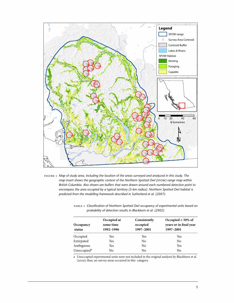
Occupancy Data for Northern Spotted Owls Researchers with the British Columbia Ministry of Environment have undertaken detection surveys for the Northern Spotted Owl throughout its range in British Columbia since 992. Each year, inventory detection surveys are conducted by broadcasting Northern Spotted Owl calls at predetermined stations along linear transects, and recording the species and locations of owls detected. For the purposes of this study, we used a sample of 40 survey areas that were previously analyzed by Blackburn et al. (2002) and were based on inventory detection data col-lected in 992–200 (Figure ). Survey areas had been defined by Blackburn et al. (2002) using call broadcast stations on linear transects that were located in the vicinity of prior observations of Northern Spotted Owls. In the analyses, we refer to these survey areas as “experimental units” (EUs). EUs can vary in area depending on the lengths of transects surveyed, and they have varied numbers of detection points.

The resulting data can be used to determine the presence of Northern Spotted Owls within an area surrounding each station. Based on communi-cation with one of the biologists who has been conducting the surveys (J. Hobbs, B.C. Ministry of Environment, pers. comm., June 2006), we assumed that a 500-m buffer around each station represents the effective area sampled for that station. Beyond this distance it is unlikely that the researcher will de-tect owl responses to the broadcast call. Based on the number of stations sampled, a measure of sampling effort was calculated for each of the EUs rep-resented by transect(s) surveyed within them. A probability of detection of Northern Spotted Owl was then assigned to each EU based on sampling ef-fort. According to the standardized survey methodology used by Blackburn et al. (2002), absence of Northern Spotted Owls along a given transect or within an EU represented by several transects, was inferred when no call-backs were received after a specified level of sampling effort.

Classification of Northern Spotted Owl Occupancy of Experimental UnitsBlackburn et al. (2002) did not report a metric for occupancy or occupancy categories that we could use for comparative analysis in this study; therefore, we first developed a simple classification of occupancy of the EUs using the authors’ probability of detection estimates (Table ). For a particular survey year, we considered an EU to be vacant if no owl was detected and there was at least a 90% chance of detecting an owl if it were present, based on Black-burn et al.’s (2002) analysis of sampling effort. We reinterpreted the authors’ original occupancy classes to create a simple indicator of degree of change in occupancy status by arbitrarily splitting the inventory data into two equal time blocks of 5 years, as follows:

) Occupied: ongoing 992–200 (combining the 992–996 and 997–200 determinations of EUs classed as Occupied),

2) Extirpated: initially occupied (992–996) but not detected later (997–200), and assumed to be vacated in that second time interval,

5

�

�

�

��

�

�

�

�

�

�

�

�

�

�

�

�

�

�

�

�

�

�

�

�

�

�

�

�

�

�

�

�

�

�

�

�

�

�

9

8

7

6

54

3

2

140

39

38

36

35

34

33

32

31

30

29

28

27

26

25

24

2322

21

20

19

18

17

16

1514

13

12

11

10

������

�

����������

��������������������

��������������

��������������

������������

�������

��������

�������

0 20 40 6010K ilometres

¹

Figure 1 Map of study area, including the location of the areas surveyed and analyzed in this study. The map insert shows the geographic context of the Northern Spotted Owl (SPOW) range map within British Columbia. Also shown are buffers that were drawn around each numbered detection point to encompass the area occupied by a typical territory (5-km radius). Northern Spotted Owl habitat is predicted from the modelling framework described in Sutherland et al. (2007).

Table 1 Classification of Northern Spotted Owl occupancy of experimental units based on probability of detection results in Blackburn et al. (2002)

Occupied at Consistently Occupied ≥ 50% ofOccupancy some time occupied years or in final year status 1992–1996 1997–2001 1997–2001

Occupied Yes Yes YesExtirpated Yes No NoAmbiguous Yes No YesUnoccupieda No No No

a Unoccupied experimental units were not included in the original analysis by Blackburn et al. (2002); thus, no survey areas occurred in this category.

6

3) Ambiguous: occupied at some point between 992 and 996 and detected in at least 50% of the years from 997 to 200 or in the final year 200, but lacked a pattern of occupancy that was consistent enough to class as either Occupied or Extirpated, and

4) Unoccupied: no detections between 992 and 200.

The survey methodology used by Blackburn et al. (2002) did not permit estimation of a probability of colonization of new areas after the surveys began.

Estimation of Habitat Quantity and ConnectivityQuantity of Suitable Habitat We used three different methods for calculat-ing the area of suitable habitat1 associated with a particular EU to explore the effects of differing spatial extents (hereafter termed “scale of resolution”) over which habitat suitability could be interpreted. We present these methods in order of increasing area encompassed, although they differ in other ways be-yond simple area-scaling interpretations. For each method, we calculated the amount of nesting and foraging habitat within the encompassed area (buffer). In general, the amounts of nesting and foraging habitat were highly correlat-ed, so we restricted our comparative analyses to a single indicator of suitable habitat quantity defined as the proportion of nesting and foraging habitat.

. Detection Radius – We calculated a circular buffer with a 500-m radius around each detection point. This radius was chosen to capture the total area within which the detected bird may have actually occurred, based on the distance over which the researcher could have heard a Northern Spot-ted Owl response to the call-back tapes. This buffer distance is an imprecise estimate of actual detection distance for a particular point, which can be affected by factors such as topography and weather condi-tions. This is the smallest and most conservative of the three methods in terms of the area sampled.

2. Territory Radius – We used a circular buffer with a 5000-m radius around each detection radius, which is intended to encompass the area of a typical Northern Spotted Owl territory (see Sutherland et al. 2007). A circle is an imperfect representation of an actual territory because its shape is likely related to topography, amount of suitable habitat, and location of adjacent territories. Thus, we expect that this buffer could include substantial areas of non-suitable habitat.

3. Intersection of Projected Territories Radius (hereafter referred to as Inter-secting Territories Radius) – We used the territory model component of the modelling framework (Sutherland et al. 2007) to project the location and spatial configuration of feasible territories that intersected a 5000-m buffer around each detection point. This approach is intended to reflect habitat quantity of projected territories from which the detected bird, as represented by the detection point, could have originated. The indicator accounts for current understanding of Northern Spotted Owl behaviour by including factors known to be associated with this species’ habitat use and territory shape.

Suitable habitat for nesting and foraging is aged respectively as 40 yrs and 20 yrs for the Mari-time, 0 yrs and 00 yrs for the Submaritime, and 00 yrs and 80 yrs for the Continental ecological subregions (see Sutherland et al. 2007).

7

Projected territories were generated for two different landscape scenarios: () current landscape conditions (i.e., 2004), and (2) recreated landscape conditions 20 years in the past (i.e., 984). The configuration of the historic landscape was estimated by converting all stands logged within the last 20 years to old growth. Our assumption that all harvested stands were old growth at the time of harvest likely overestimates the age of the forest. Stands harvested in the last 20 years would likely include some mature forest. But given the general nesting and foraging habitat definitions cur-rently used for Northern Spotted Owls, this forest would still have been suitable for the owls. We used a reconstruction because reliable and com-parable inventory data from that time period were not available for spatial modelling. We chose 20 years for the historic scenario to reflect an upper limit of the expected duration of nest site fidelity. Specifically, we estimat-ed the average generation time for a Northern Spotted Owl in the wild (~0 years [Courtney et al. 2004]; assumption used in Sutherland et al. 2007), and doubled it to account for intergenerational nest site fidelity. This reconstruction of a “historical” situation was expected to be more informative relative to current conditions because it reflects territory locations based on the expected arrangement of habitat at the time the previous set of territories were established (assumed to influence the prob-ability of detection), which allows us to better relate habitat loss to occupancy patterns. We used single runs from each of the scenarios, a method that ignores the effect of stochastic parameters used in the territo-ry formation model.

Testing Model Classifications of Suitable Habitat at Different Scales To test H-, we compared the weighted mean proportions of suitable habitat found at detection points within each survey area classed as Occupied (i.e., Occu-pied EU) to the mean proportions of suitable habitat found at the three scales of resolution around 200 points placed completely at random within the overall study area (where the area around each random location equals an EU, termed “Random EU”, for the analysis). We made comparisons at three scales: Detection Radius, Territory Radius, and Intersecting Territories Radi-us. Random EUs could potentially overlap the EUs at one or more of the three scales. We weighted the mean proportion of each Occupied EU using the total area (ha) of the EU. If the buffer around a detection location overlapped the edge of the range limit for the Northern Spotted Owl, it was extended to include areas outside the range boundary (consistent with Sutherland et al. 2007), and this added area was included in the total area for the EU.

Habitat Connectivity among Experimental Units We compared how well each EU was connected to the entire network of EUs by using existing meth-ods for calculating connectivity (outlined in Sutherland et al. 2007) and extending them for this analysis. First, we placed a single point in the centre of all the detection points plotted in an EU (i.e., calculated as the mean lati-tude and longitude of the detection points for that unit). A node in the connectivity framework was represented by either the habitat patch (i.e., ≥ 0 ha) containing the mean point or the closest habitat patch to the mean point. Connectivity costs between all pairs of nodes were calculated as the least-cost path through the connected network (i.e., the minimum planar graph), where the least-cost paths were determined based on the methods for esti-

8

mating movement costs for a Northern Spotted Owl as a function of land cover type, stand age, and stand structure (Table 2 in Sutherland et al. 2007).

An overall index of connectivity was assigned to each EU as the harmonic mean of the least-cost distance between the node associated with that unit and all other nodes in the network. In this context, the harmonic mean least- cost distance is the reciprocal of the arithmetic mean of the reciprocal pair-wise least cost distances among the set of nodes. Use of this method to estimate connectivity of a particular EU accounts for the diminishing proba-bility that Northern Spotted Owls would encounter potential territories at large cost distances (i.e., very isolated areas of habitat). That is, we assumed that nodes that were near other nodes were more likely to be classed as Occu-pied EUs than nodes that were more isolated from other nodes.

Data Analyses

Before testing our hypotheses we made the following simplifications to the data:

. We grouped EUs classed as Ambiguous with those classed as Extirpated based on visual examination of the degrees of overlap between Gaussian plots (Appendix A), and on the results of fixed effects two-way ANOVAs. These showed that the amount of suitable habitat for EUs classed as Am-biguous was not significantly different from EUs classed as Extirpated, treating scale as a covariate (F0.05, ,54 = 0.003, p = 0.96). Similarly, the connectivity between EUs classed as Ambiguous compared with those classed as Extirpated was not significantly different (F0.05, ,54 = 0.6, p = 0.69), again treating scale as a covariate.

2. It is possible that the same owl was detected in EUs that were very near one another. Thus, apparent extirpations could be the result of an owl moving from one area to another rather than to loss of habitat or interfer-ence with other owls. By visual inspection we determined that the patterning of occupancy classes in relation to the habitat covariates was strengthened when proximate EUs were grouped (see Figure A-2). In gen-eral, EUs with high quantities of suitable habitat that were individually classed as Extirpated occurred adjacent to Occupied EUs with high quanti-ties of suitable habitat. This result is consistent with the hypothesis that “extirpations” within closely grouped EUs are not necessarily due to changes in habitat covariates (e.g., habitat loss), and may instead be related either to movements of owls or effects of other threats on overall popula-tion numbers, or are simply artifacts of survey area delineation. To reduce this effect in our analysis, we grouped together EUs whose centroids (nodes) were within one territory radius (5 km) of one another (Appendix A). We applied the highest class of occupancy found within the group to each EU that was a member of the group (i.e., Occupied > Ambiguous > Extirpated).

3. Two EUs containing large outlier values for connectivity were retained for simple graphical comparisons (see Appendix A), but were removed for statistical comparisons.

4. For analyses, we removed Random EUs in which the unit did not overlap any projected territories. If this occurred, there would be no valid value for the amount of suitable habitat in territories for that EU. This rare event could occur because the location of territories shifts as a function of

9

changing habitat amounts, and it is not guaranteed that these overlaps ac-tually occur where EUs occur.

As described above, we used the survey area as the experimental unit for statistical analyses because detection points were nested within survey areas and so cannot be treated as independent observations. We calculated habitat indicator values using the average value for all detection points within an EU. Random points were treated as independent sample units; hence, they were treated as both sampling units and EUs in analyses. Before analysis, we trans-formed all proportions using the arcsine transformation, and tested for departures from normality before using parametric analyses.

Testing Model Classifications of Suitable Habitat at Different Scales For tests of the models’ classifications of suitable habitat (H), we used two- sample t-tests and two-way analysis of variance (ANOVA) to compare classifications of habitat within and among EUs, random points, and scales of analysis.

Inter-period Patterns of Experimental Unit Occupancy We used two ap-proaches for testing inter-period patterns of occupancy (H2). For our first approach we estimated Gaussian bivariate ellipses of the sample data. The re-sulting ellipses were centred on the unweighted sample means of two variables: the proportion of suitable habitat, and the least-cost distance to other EUs. The sample standard deviations of the two variables determine the major axes, and the sample covariance determines the orientation of each el-lipse. Ellipses enclose the area defined by the 0.683 probability contour for the sample data. This probability value represents the central confidence in-terval for approximately Gaussian probability density functions (Cowan 998).

For our second approach we first assessed the relative effects of the two factors (habitat suitability 2004 and habitat connectedness 2004, 984) on the occupancy class assigned to each EU at each scale using logistic regression. The general logistic model we used was:

logit(θsi ) = β0+ βsxsi + β2sx2si + β3s(xsi * x2si ) ()

where logit θsi expresses the probability of EU i being classed as Occupied, as a function of habitat covariates projected for that EU i calculated at a par-ticular spatial scale s, and consisting of the EU’s habitat suitability (xi) and the measure of connectivity (x2i). The coefficients (βs) are estimated. We assessed the significance of each coefficient in the model using a quasi- maximum likelihood version of the Wald test. Second, we further compared the differences in both connectivity and habitat amounts at each scale be-tween 984 and 2004 at EUs classed as Occupied or Extirpated. For this latter comparison, we used two-sample t-tests, and for tests using the proportion of suitable habitat as the response variable, we used arcsine transformed pro-portions.

All statistical tests were conducted using SYSTAT-0™ (SPSS Inc. 2000).

Results

Testing Model Classifications of Suitable Habitat at Different Scales At all three scales we tested (Detection Radius, Territory Radius, Intersecting Terri-

0

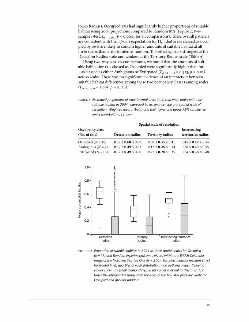
tories Radius), Occupied EUs had significantly higher proportions of suitable habitat using 2004 projections compared to Random EUs (Figure 2; two- sample t-test: tα = 0.05, p < 0.000 for all comparisons). These overall patterns are consistent with the a priori expectation for H- that areas classed as occu-pied by owls are likely to contain higher amounts of suitable habitat at all three scales than areas located at random. This effect appears strongest at the Detection Radius scale and weakest at the Territory Radius scale (Table 2).

Using two-way ANOVA comparisons, we found that the amounts of suit-able habitat for EUs classed as Occupied were significantly higher than for EUs classed as either Ambiguous or Extirpated (F0.05, , = 6.923, p = 0.0) across scales. There was no significant evidence of an interaction between suitable habitat differences among these two occupancy classes among scales (F0.05, 2, = 2.093, p = 0.28).

Figure 2 Proportion of suitable habitat in 2004 at three spatial scales for Occupied (N =19) and Random experimental units placed within the British Columbia range of the Northern Spotted Owl (N = 200). Box plots indicate medians (thick horizontal line), quartiles of each distribution, and outlying values. Outlying values shown by small diamonds represent values that fall farther than 1.5 times the interquartile range from the ends of the box. Box plots are white for Occupied and grey for Random.

���

���

���

���

���

�

����

�����

�������

�������

����

� ���������� ���������� ������������������������� ������� ������� ������

Table 2 Estimated proportions of experimental units (EUs) that were projected to be suitable habitat in 2004, expressed by occupancy type and spatial scale of resolution. Weighted means (bold) and their lower and upper 95% confidence limits (non-bold) are shown

Spatial scale of resolutionOccupancy class Intersecting(No. of EUs) Detection radius Territory radius territories radius

Occupied (N = 19) 0.52 ≤ 0.60 ≤ 0.68 0.30 ≤ 0.35 ≤ 0.41 0.45 ≤ 0.49 ≤ 0.54Ambiguous (N = 7) 0.37 ≤ 0.49 ≤ 0.61 0.17 ≤ 0.26 ≤ 0.34 0.26 ≤ 0.40 ≤ 0.55Extirpated (N = 13) 0.37 ≤ 0.49 ≤ 0.60 0.22 ≤ 0.28 ≤ 0.35 0.24 ≤ 0.36 ≤ 0.48

Inter-period Patterns of Experimental Unit Occupancy Overall, we found some evidence that suggested significant relationships exist between occu-pancy class and () proportion of suitable habitat, (2) connectivity among EUs, and (3) interactions between proportions of suitable habitat and connec-tivity, although this evidence could not be demonstrated across all scales or among the time periods we examined (Table 3; see also Figure 3). In particu-lar, for the 2004 landscape, Occupied EUs contained significantly higher proportions of suitable habitat and greater connectivity between habitat patches than those classed as either Extirpated or Ambiguous at the smallest spatial scale of resolution (Detection Radius) based on parameter estimates. However, this tendency did not extend to the more aggregated scales of Terri-tory Radius or Intersecting Territories Radius. For the reconstructed 984 landscape, this same set of relationships could not be statistically demon-strated at any scale, although at the scale of Territory Radius, there was a significant positive association between proportions of suitable habitat and occupancy status of EUs (Figure 3; Table 3). At all scales and time periods, there was considerable overlap in the habitat characteristics of EUs in each occupancy class (Figure 3). We note that the statistical power of these tests was likely low due to small sample sizes (sample sizes are shown in Figure 3). Accordingly, these findings must be interpreted cautiously.

We found no evidence that declines in connectivity among patches of suitable habitat between 984 and 2004 were more strongly associated with Extirpated EUs than Occupied EUs (two-sample t-test: tα = 0.05, df = 30 = -0.24, p = 0.8). Similarly, except at the scale of Intersecting Territories Radius, we found no evidence that changes in habitat amounts between 984 and 2004

Table 3 Parameter estimates and model success in predicting occupancy class at the different spatial scales and time scales assessed. Parameter estimates are shown on the logit scale, with model-specific p values shown below each parameter

Model Habitat Habitat Connectivity suitability Model suitability between and Likelihood- prediction effect units effect connectivity ratio successYear Scale Constant (β1) (β2) (β3) statistica probabilityb

2004 Detection 14.71 -19.17 -0.00 0.00 15.67 0.69 radius (p = 0.05) (p = 0.07) (p = 0.03) (p = 0.04) (p < 0.01) Territory -3.41 17.01 0.00 -0.00 11.36 0.65 radius (p = 0.46) (p = 0.22) (p = 0.65) (p = 0.30) (p = 0.01) Intersecting 13.15 -16.91 -0.00 -0.00 11.39 0.64 territories (p = 0.28) (p = 0.41) (p = 0.25) (p = 0.40) (p < 0.01) radius

1984 Detection 0.60 -0.02 -0.00 -0.00 3.79 0.56 radius (p = 0.75) (p = 0.99) (p = 0.20) (p = 0.37) (p = 0.29) Territory -3.91 12.15 0.00 0.00 8.09 0.61 radius (p = 0.07) (p = 0.03) (p = 0.55) (p = 0.30) (p = 0.04) Intersecting 3.50 -4.58 -0.00 0.00 2.37 0.62 territories (p = 0.17) (p = 0.24) (p = 0.11) (p = 0.11) (p = 0.51) radius a The likelihood ratio tests the null hypothesis that all coefficients in the fitted model, except the constant, are 0. b This represents the estimated probability of correctly classifying new cases given the input data set.

2

Figure 3 Relationship between projected habitat connectivity among survey areas and the proportion of area that is suitable habitat at three spatial scales (top to bottom) and two temporal scales (left to right) for the 1992–2001 Northern Spotted Owl experimental units classed into occupancy classes. Shown is the 68.3% probability contour outlining the central confidence region of a Gaussian bivariate ellipse for units that have been grouped (see text). For each ellipse, the centre is represented by the sample means of the two variables, the vertices and co-vertices are functions of the standard deviations and covariance between the two variables, and the orientation depends on whether the covariance is positive or negative.

� ��� ��� ��� ��� ��� ��� ��� ����

��

��

��

��

���

��������������������������������������

������

�� ������������������������������

���������������������������

� ��� ��� ��� ��� ��� ��� ��� ����

��

��

��

��

���

��������������������������������������

������

�� ������������������������������

���������������������������

� ��� ��� ��� ��� ��� ��� ��� ����

��

��

��

��

���

��������������������������������������

������

�� ������������������������������

���������������������������

� ��� ��� ��� ��� ��� ��� ��� ����

��

��

��

��

���

��������������������������������������

������

�� ������������������������������

���������������������������

� ��� ��� ��� ��� ��� ��� ��� ����

��

��

��

��

���

��������������������������������������

������

�� ������������������������������

���������������������������

� ��� ��� ��� ��� ��� ��� ��� ����

��

��

��

��

���

��������������������������������������

������

�� ������������������������������

���������������������������

(2004 landscape) n = 37 (reconstructed 1984 landscape) n = 37

(2004 landscape) n = 37 (reconstructed 1984 landscape) n = 37

(2004 landscape) n = 37 (reconstructed 1984 landscape) n = 37

Detection Radius

Territory Radius

Intersecting Territories Radius

3

were associated with changes in occupancy status (two-sample t-tests com-paring suitable habitat among Occupied EUs vs. Extirpated EUs at the scales of Detection Radius: tα = 0.05, df = 30 = 0.5, p = 0.88; Territory Radius: tα = 0.05, df = 30 = -0.42, p = 0.68; Intersecting Territories Radius: tα = 0.05, df = 30 = -2.348, p = 0.03). For the latter scale (Intersecting Territories Radius), Extir-pated EUs showed higher amounts of suitable habitat in 2004 compared with 984, and compared with Occupied EUs in both time periods.

DISCUSSION

Overall, our analyses revealed that areas where Northern Spotted Owl EUs maintained their status as Occupied over the time period we examined (992–200) occurred where the model classified habitat to be of equal or higher quality (measured as proportions of suitable habitat) and more closely connected (lower average mean least-cost distances between patches of suit-able habitat) than was the case in areas where EU occupancy status became Ambiguous or Extirpated. This was true both for locations chosen at random and areas where Northern Spotted Owls had become extirpated or their sta-tus was ambiguous. Characteristics of Extirpated EUs or Ambiguous EUs were more similar to Random EUs than were Occupied EUs. Although varia-tion in the projected habitat characteristics among EU classes was quite wide, these results are consistent with those of other studies on Northern Spotted Owls (e.g., Meyer et al. 998), and they suggest that the habitat models are identifying habitat characteristics that are likely correlated with observed oc-cupancy of areas by Northern Spotted Owls in British Columbia (H).

However, our results are less revealing about the behavioural mechanisms of habitat selection by Northern Spotted Owls in this northern portion of their range. For example, do owls chose a suitable landscape and then look for a place to nest, or do they locate a suitable nest and then evaluate the sur-rounding landscape? Our a priori expectation was that these relationships might be most apparent at the largest spatial scale of analysis (Intersecting Territories Radius) and least observable at the smallest spatial scale (Detec-tion Radius) based on the assumption that owls may use a hierarchical habitat selection process from coarse-grained to increasingly fine-grained. But we cannot statistically separate the strength of the responses of Northern Spotted Owls (as measured by occupancy status) between spatial scales of resolution given current data and methods.

The hypothesis that inter-period patterns of occupancy by Northern Spot-ted Owls are related to available habitat at multiple spatial scales (H2) appears to be only partially supported by our findings. Specifically, in the 2004 land-scape, we found statistically significant positive relationships between proportions of suitable habitat and connectivity in areas classed as Occupied at the finest-grained spatial scale of Detection Radius, but the relationship was weaker at the coarser-grained scales of Territory Radius or Intersecting Territories Radius (i.e., the models were significant but the individual param-eters were not). Conversely, using the 984 reconstructed landscape, we found that proportion of suitable habitat (but not connectivity) appeared sig-nificantly greater for Occupied EUs at the Territory Radius scale, but was not significantly greater at either the Intersecting Territories Radius or Detection

4

Radius scales. Although we are cautious in interpreting these results, they are consistent with observations elsewhere and with the idea that owls are more likely to continue to occupy areas of higher quality habitat for nesting, even if those areas are small (J. Buchanan, Washington Department of Fish and Wildlife, pers. comm., Oct. 2009). At least in the 2004 landscape, certainty of patch use may be highest at nest sites, and it generally decreases as the scale of analysis includes more area farther from the nest, but how habitat patches or habitats are selected is clearly a more complex process than our analyses can illuminate. The results for the Intersecting Territories Radius scale using the reconstructed 984 landscape also suggest that owls show fidelity to larger areas that previously had higher proportions of suitable habitat, even if that habitat had diminished over time, although we cannot confirm from our re-sults that this is occurring. Marking studies have shown that many of the owls detected on surveys are older (J. Hobbs, B.C. Ministry of Environment, pers. comm., Nov. 2005), and site fidelity could be a factor in determining whether owls continue to occupy an area. However, these suggestions require further testing with marked individuals before firmer conclusions can be drawn.

The hypothesis that occupancy of areas by Northern Spotted Owls in Can-ada is at least partially related to the amount and distribution of suitable habitat as classified by the models appears to be at least partially supported. However, the more specific hypothesis that inter-period declines in either habitat quality and/or habitat connectivity may be correlated with the decline of the Northern Spotted Owl in British Columbia since 992 is not clearly supported by our results. Interestingly, contrary to the general expectations for H2, we found that EUs classed as Extirpated had significantly higher pro-portions of suitable habitat in 2004 than in 984 at the scale of Intersecting Territories Radius, although not at finer scales. We suggest four possibilities to account for this finding. One is that while habitat suitability may have in-creased at the most aggregated scale we measured (Intersecting Territories Radius), at finer scales (e.g., Territory Radius) it has actually become more interspersed with harvest cutblocks, and thus the contiguity of nesting habi-tat may have actually decreased during this period. If so, owls may be less likely to remain in patches of nesting habitat or may become more difficult to detect during surveys (a “habitat dilution” effect). A second and related pos-sibility is that a general decline in detectability of Northern Spotted Owls occurred over the time frame of this analysis, which reduced the power of the tests to detect differences (see below). A third possibility is that the negative effects of other threats to Northern Spotted Owls in the study area (e.g., Barred Owls [Strix varia]), outweighed any observable positive effects of hab-itat improvement on occupancy by Northern Spotted Owls. Barred Owls are a significant competitive threat to Northern Spotted Owls throughout their range (Gutiérrez et al. 2007). Densities of Barred Owls have been increasing in British Columbia since the 940s. The habitat requirements of the two spe-cies show considerable overlap (Smith et al. 2008). Barred Owls may also use habitat patches required by Northern Spotted Owls as well as patches of for-est that are not suitable for Northern Spotted Owls. Finally, it is possible that our definition of suitable habitat, extrapolated from studies obtained largely from the United States (see Sutherland et al. 2007), is less accurate at the lower bound of suitability (particularly for habitat that is recovering from disturbance) than for forests that have not been disturbed or have had more

5

time to recover habitat values. Thus, our results cannot and do not exclude other causal explanations besides reductions in habitat amount and connec-tivity for the general declines in area occupancy.

There is a significant effect of scale-dependency in our results—i.e., some patterns appear clearest and most broadly consistent with our a priori expec-tations at the most extensive geographic scale (Intersecting Territories Radius) and at the smallest and most localized scale (Detection Radius), but are less consistent and more variable at intermediate scales (Territory Radi-us). Possible explanations for this include the following: First, at the smallest scale (i.e., the 80-ha scale of Detection Radius), Northern Spotted Owls are likely to prefer locations that have at least a minimum proportion of suitable habitat. Second, at larger scales (i.e., Territory Radius), non-habitat is likely to be included, which reduces the overall proportion of possible suitable habitat in a territory area. Third, the model algorithm for projecting territoriessearches for suitable habitat that meets minimum criteria for different attri-butes. Therefore, if the algorithm adequately captures the same criteria used by Northern Spotted Owls, then areas of intersection between adjacent pro-jected territories (i.e., Intersecting Territories Radius) may relate to large- scale habitat selection processes, including social factors for finding mates (LaHaye et al. 200), and therefore reflect occupancy status.

At the scale of projected territories (approximated by the buffer used to create the Territory Radius unit), the Northern Spotted Owl Analysis Frame-work (Sutherland et al. 2007) generates territories based on the configuration of the current landscape. In this model, territories are initiated at “active sites”, and these projected territories can be either occupied or previously oc-cupied by owls. We have not confirmed if areas in which owls become extirpated are more likely to occur where the model framework cannot form viable territories. However, for the analysis that compared occupancy class with quality of adjacent intersecting territories, we used the locations of terri-tories projected by the model framework based on a configuration of habitat that was similar to that which could have been present when the territory was established (i.e., at the beginning of the time period we assessed). This histor-ic perspective on projected territory locations allowed us to account for projected territories that may have subsequently declined in quality due to anthropogenic or natural disturbance. Nonetheless, the accuracy of this ap-proach could be improved by incorporating empirical estimates of the typical duration of nest fidelity following habitat degradation, and by studies that evaluate the abundance and availability of prey in habitat patches used by Northern Spotted Owls.

In this study, we focussed on habitat suitability and connectivity as the two main factors that contribute to the differences in the likelihood that Northern Spotted Owls occupy areas of habitat (i.e., annual territories) for successive years. These factors are generally expected to be related to the ability of Northern Spotted Owls to meet their life and breeding requirements in the landscape (e.g., suitability with survival and reproduction [Sutherland et al. 2007 and references cited therein], and connectivity influencing local popula-tion dynamics [O’Brien et al. 2006]). However, other factors may contribute to patterns of variation and heterogeneity in territory occupancy data for Northern Spotted Owls. For example, detectability may have declined over the time period covered by this study due to population declines that were not related to habitat quality and connectivity (e.g., behavioural responses to

6

threats from Barred Owls). At present, numbers of Northern Spotted Owls are very low in the study area (see Sutherland et al. 2007). Therefore, it is pos-sible that local effects of stochastic factors (e.g., effects of predation, winter severity, etc.) have come to dominate the current distribution patterns of Northern Spotted Owls in British Columbia. However, estimating the effects of stochastic factors on detectability errors was not part of our analysis of the occupancy data.

Our primary purpose in this study was to verify model assumptions used in Sutherland et al. (2007) and not to build a predictive habitat occupancy model for Northern Spotted Owls in Canada. Therefore, we did not attempt to use a full model estimation approach, such as the state-space approaches developed by others (Wintle et al. 2003; Mackenzie et al. 2005), to estimate the probability of each unit occurring in each occupancy class. For example, the time period of interest included multiple years (992–200); the chances of detecting Northern Spotted Owls during this period may have diminished due to a decline in the population that was unrelated to the tested factors, which could have contributed to heterogeneity. Changes in detectability (e.g., due to the presence of Barred Owls) may also have contributed to the observed heterogeneity in occupancy status, although estimating this error was not considered in our analysis. Our results should be treated as an explo-ration of the implications of important assumptions rather than as strict tests of the influence of habitat variables on trends in population occupancy.

Despite the fact that we are not able to directly test ecological hypotheses about the relationship between resource abundance and habitat selection in this Northern Spotted Owl population, we think that our analyses demon-strate that the assumptions in the habitat components of the model frame-work are consistent with the empirical data, and do improve confidence in the model structure. By understanding the key habitat-population assump-tions, decision-makers that use this or similar models are in a stronger posi-tion to make informed management decisions based on probable outcomes of current or future management policies.

LIMITATIONS OF THIS STUDY

At the outset of our analysis we recognized some important limitations in the data that imposed constraints on the statistical inferences available to us in testing our hypotheses. These limitations included () small sample size, (2) annual variations in the sampling design used to select transect locations, (3) annual variation in sampling effort within Northern Spotted Owl detection surveys, and (4) non-random and non-stratified sampling of the landscape. We attempted to overcome the effects of some of these limitations by various means: our classification of occupancy, methods of comparing habitat amounts, and use of a priori expectations to guide interpretation of results and tests. However, we caution that our results are properly treated as an exploration of the implications of important assumptions rather than as sufficient tests of the influence of habitat variables on population trends.

Our analysis was based on independent sets of quantitative data. The only potential dependency between these data sets is that the field study and prior analysis of area occupancies pre-dated the development of the model frame-

7

work. The findings from the field study may have informed the expert opinion that contributed to portions of the simulation model specifications.

We do not have an independent method of directly estimating the strength of the relationship between modelled and actual habitat quality for sampled EUs. As an alternative, we used the model to () classify habitat into types that reflected the life requisite functions that support Northern Spotted Owls, (2) assess the abundance of each type at different scales, and (3) use those esti-mates in an analysis of historical patterns of occupancy. As discussed above, we did not have data on other factors (i.e., threats) that may also be influenc-ing changes in area occupancy. Therefore, we cannot test directly either H or H2, although we can test whether the results are in the predicted direction (thus fulfilling our objective of exploring assumptions).

Many current methods of quantitatively estimating occupancy status are designed to make direct estimates of probability of detection (Mackenzie et al. 2005; Wintle et al. 2005). In our case, the probabilities of detection had al-ready been estimated by Blackburn et al. (2002). Therefore, we used their estimates to create occupancy classes rather than produce our own probabili-ties of detection. By doing so, we did not attempt to construct full likelihood or state-space models of the probability of detection (see Mackenzie et al. 2006) because we could not reconstruct the complete detection histories of the original samples, nor could we fully re-characterize the sources of error in the original estimation of the probability of detection.

Our analyses of habitat quantity are intended to identify relationships be-tween the amount of habitat occurring in the vicinity of a detection point and the occupancy class of the habitat unit (i.e., a projected territory) containing that point. While we expect that the amount of habitat within a projected ter-ritory is related to its suitability for meeting the territory holder’s life history requirements, we were uncertain about the most appropriate scale at which to measure quantity of habitat for our analyses. Furthermore, we recognize that the suitability of habitat is related to its spatial configuration, in addition to quantity. We also assumed, as was done in the model framework, that within each occupancy class, the territories are functionally equivalent within the range of variation sampled. If some territories, in either class, were more productive than others for contributing to the Spotted Owl population, that was not accounted for in the verification testing or in the model framework.

8

LITERATURE CITED

Blackburn, I., A.S. Harestad, J.N.M. Smith, S. Godwin, R. Henze, and C.B. Lenihan. 2002. Population assessment of the Northern Spotted Owl in British Columbia 992–200. B.C. Min. Water, Land and Air Protection, Victoria, B.C. Unpub. Rep. www.env.gov.bc.ca/wld/documents/spow-trend_992_200.pdf (Accessed Dec. 2, 2009).

Bunnell, F.L. and M. Boyland. 2003. Decision-support systems: it’s the ques-tion not the model. J. Nature Conservation 0: 269–279.

Chutter, M.J., I. Blackburn, D. Bonin, J. Buchanan, B. Costanzo, D. Cunning-ton, A. Harestad, T. Hayes, D. Heppner, L. Kiss, J. Surgenor, W. Wall, L. Waterhouse, and L. Williams. 2004. Recovery strategy for the Northern Spotted Owl (Strix occidentalis caurina) in British Columbia. B.C. Min. Environ., Victoria, B.C. www.sararegistry.gc.ca/virtual_sara/files/plans/rs_spotted_owl_caurina_006_e.pdf

Courtney, S.P., J.A. Blakesley, R.E. Bigley, M.L. Cody, J.P. Dumbacher, R.C. Fleischer, A.B. Franklin, J.F. Franklin, R.J. Gutiérrez, J.M. Marzluff, and L. Sztukowski. 2004. Scientific evaluation of the status of the Northern Spotted Owl. Sustainable Ecosystems Institute, Portland, Oreg. www.sei.org/owl/finalreport/finalreport.htm (Accessed November 2006).

Cowan, G. 998. Statistical data analysis. Oxford University Press, New York, N.Y.

Fuller, M.M., L.J. Gross, S.M. Duke-Sylvester, and M. Palmer. 2008. Testing the robustness of management decisions to uncertainty: everglades res-toration scenarios. Ecological Applications 8:7–723.

Gutiérrez, R.J., M. Cody, S. Courtney, and A.B. Franklin. 2007. The invasion of Barred Owls and its potential effect on the Spotted Owl: a conserva-tion conundrum. Biol. Invasions 9:8–96.

LaHaye, W.S., R.J. Gutiérrez, and J.R. Dunk. 200. Natal dispersal of the Spot-ted Owl in southern California: dispersal profile of an insular population. Condor 03: 69–700.

Mackenzie, D.I., J.D. Nichols, N. Sutton, K. Kawanishi, and L.L. Bailey. 2005. Improving inferences in population studies of rare species that are de-tected imperfectly. Ecology 86:0–3.

Mackenzie, D.I., J.D. Nichols, J.A. Royle, K.H. Pollock, L.L. Bailey, and J.E. Hines. 2006. Occupancy estimation and modelling: inferring patterns and dynamics of species occurrence. Elsevier Inc., New York, N.Y.

Meidinger, D. and J. Pojar. 99. Ecosystems of British Columbia. B.C. Min. For., Victoria, B.C. Spec. Rep. Ser. No. 6. www.for.gov.bc.ca/hfd/pubs/Docs/Srs/Srs06.htm

Meyer, J.S., L.L. Irwin, and M.S. Boyce. 998. Influence of habitat abundance and fragmentation on Northern Spotted Owls in western Oregon. Wildlife Monogr. 39:–5.

9

O’Brien, D.T., M. Manseau, A. Fall, and M-J. Fortin. 2006. Testing the impor-tance of spatial configuration of winter habitat for woodland caribou: an application of spatial graph theory. Biol. Conservation 30:70–83.

Rykiel, E.J., Jr. 996. Testing ecological models: the meaning of validation. Ecological Modelling 90:299–244.

Smith, J., G.D. Sutherland, D.T. O’Brien, F.L. Waterhouse, J.B. Buchanan, J. Hobbs, and A.S. Harestad. 2008. Relationships between elevation and slope at Barred Owl sites in southwestern British Columbia. B.C. Min. For. Range, Res. Section, Coast Forest Region, Nanaimo, B.C. Tech. Rep. TR040. www.for.gov.bc.ca/rco/research/Wildlifereports/TR40%20barred%20all4.pdf (Accessed Feb. 5, 200).

Sutherland, G.D., D. O’Brien, A. Fall, F.L. Waterhouse, A.S. Harestad, and J.B. Buchanan. 2007. A framework to support landscape analyses of habitat supply and effects on populations of forest-dwelling species: a case study based on the Northern Spotted Owl. B.C. Min. For. Range, Res. Br., Victoria, B.C. Tech. Rep. 038. www.for.gov.bc.ca/hfd/pubs/Docs/TR/Tr038.htm

SPSS Inc. 2000. SYSTAT-0. Chicago, Ill.

Wintle, B.A., R.P. Kavanagh, M.A. McCarthy, and M.A. Burgman. 2003. Esti-mating and dealing with detectability in occupancy surveys for forest owls and arboreal marsupials. J. Wildlife Manag. 69: 905–97.

20

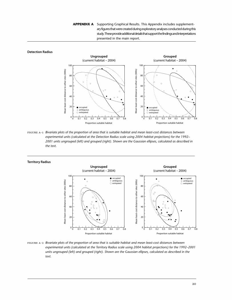
APPENDIX A Supporting Graphical Results. This Appendix includes supplement-ary figures that were created during exploratory analyses conducted during this study. These provide additional details that support the findings and interpretations presented in the main report.

Figure A-1 Bivariate plots of the proportion of area that is suitable habitat and mean least-cost distances between experimental units (calculated at the Detection Radius scale using 2004 habitat projections) for the 1992–2001 units ungrouped (left) and grouped (right). Shown are the Gaussian ellipses, calculated as described in the text.

� ��� ��� ��� ��� ��� ��� ��� ����

��

��

��

��

�����������������������������������������

������

��

���������������������������

���������������������������

� ��� ��� ��� ��� ��� ��� ��� ����

��

��

��

��

���

��������������������������������������

������

��

���������������������������

���������������������������

Ungrouped(current habitat – 2004)

Grouped(current habitat – 2004)

Detection Radius

Figure A-2 Bivariate plots of the proportion of area that is suitable habitat and mean least-cost distances between experimental units (calculated at the Territory Radius scale using 2004 habitat projections) for the 1992–2001 units ungrouped (left) and grouped (right). Shown are the Gaussian ellipses, calculated as described in the text.

� ��� ��� ��� ��� ��� ��� ��� ����

��

��

��

��

���

��������������������������������������

������

��

���������������������������

���������������������������

� ��� ��� ��� ��� ��� ��� ��� ����

��

��

��

��

���

��������������������������������������

������

��

���������������������������

���������������������������

Ungrouped(current habitat – 2004)

Grouped(current habitat – 2004)

Territory Radius

2

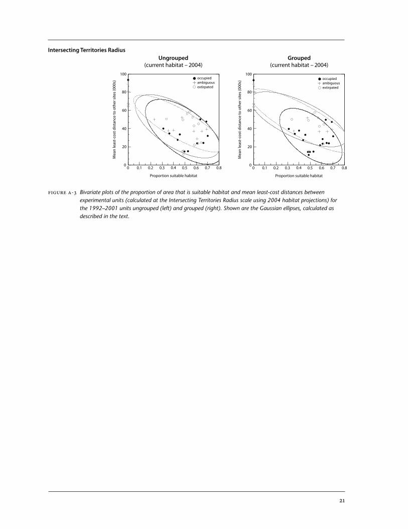
Figure A-3 Bivariate plots of the proportion of area that is suitable habitat and mean least-cost distances between experimental units (calculated at the Intersecting Territories Radius scale using 2004 habitat projections) for the 1992–2001 units ungrouped (left) and grouped (right). Shown are the Gaussian ellipses, calculated as described in the text.

� ��� ��� ��� ��� ��� ��� ��� ����

��

��

��

��

���

��������������������������������������

������

��

���������������������������

���������������������������

� ��� ��� ��� ��� ��� ��� ��� ����

��

��

��

��

���

��������������������������������������

������

��

���������������������������

���������������������������

Ungrouped(current habitat – 2004)

Grouped(current habitat – 2004)

Intersecting Territories Radius