valuation of double barrier options in heston’s...
TRANSCRIPT

Valuation of Double Barrier Options in Heston’s Stochastic Volatility Model
Using Finite Element Methods
Copyright © Changwei Xiong 2010 - 2017
Jan. 2010
last update: October 31, 2017

Changwei Xiong, October 2017 http://www.cs.utah.edu/~cxiong/
2
ABSTRACT
Heston stochastic volatility moded has been widely used in financial derivative pricing and risk
management. One of the reasons for that is that vanilla options in Heston model have close form solutions.
This makes the calibration of the model computationally much efficient and accurate. To understand these
closed form formulas, this essay in the first half will introduce the Fourier transform method for option
pricing and its application to the Heston model. Additionally, a characteristic function based method is
also discussed, which extends the Heston model to have piecewise time-dependent parameters.
Finite element method (FEM) has been developed for decades to solve partial differential
equations arise from science and engineering problems. It is well known for requiring a low order storage
and for its capability to handle complicated irregular computational domains comparing to finite
difference method (FDM). This characteristic advantage makes FEM an ideal numerical method for
valuation of exotic options. This essay in the second half will present a detailed implementation of FEM
and its application to pricing a double barrier knock-out option with an underlying asset modeled by
Heston stochastic volatility process.

Changwei Xiong, October 2017 http://www.cs.utah.edu/~cxiong/
3
TABLE OF CONTENTS
Abstract ........................................................................................................................................................2
Table of Contents .........................................................................................................................................3
1. Kolmogorov Forward and Backward Equations ..................................................................................5
1.1. Kolmogorov Forward Equation ....................................................................................................5
1.2. Kolmogorov Backward Equation ..................................................................................................8
2. Heston Model .....................................................................................................................................10
2.1. Heston Stochastic Volatility Model .............................................................................................10
2.1.1. Market Price of Risk ....................................................................................................... 10
2.1.2. Radon-Nikodym Derivative ............................................................................................ 15
2.1.3. Feller Condition ............................................................................................................... 16
2.2. Probability Distribution of Spot Returns .....................................................................................16
2.2.1. Derivation of the Transition Probability .......................................................................... 17
2.2.2. Moment Generating Function (in progress…) ................................................................ 20
2.3. Analytical Solution of Vanilla Options .......................................................................................21
2.3.1. Fourier Transform and Characteristic Function .............................................................. 21
2.3.2. Characteristic Function ................................................................................................... 25
2.3.3. Vanilla Option Prices ....................................................................................................... 29
2.3.3.1. Analogy to Cumulative Density Function ....................................................................... 29
2.3.3.2. Analogy to Probability Density Function ........................................................................ 31
2.3.3.3. Heston’s Original Solution .............................................................................................. 32
2.4. Piecewise Time Dependent Heston Model ..................................................................................35
3. Heston Model: PDE by Finite Element Method ................................................................................38
3.1. The Partial Differential Equation ................................................................................................39
3.2. Numerical Solution of the PDE ...................................................................................................42
3.2.1. Temporal Discretization .................................................................................................. 42
3.2.2. Two-Dimensional Finite Element Method ...................................................................... 43
3.2.2.1. Weak Formulation ........................................................................................................... 43
3.2.2.2. Boundary Conditions....................................................................................................... 44
3.2.2.3. Mesh and Basis Functions ............................................................................................... 46
3.2.2.4. Affine Transformation ..................................................................................................... 48
3.2.2.5. Stiffness and Mass Matrix ............................................................................................... 48
3.2.2.6. Computation of Integrals ................................................................................................. 51
3.2.3. Iterative Linear Solvers ................................................................................................... 53
3.2.3.1. Implementation of Sparse Matrix .................................................................................... 53
3.2.3.2. Iterative Methods for Asymmetric Sparse Matrix ........................................................... 54

Changwei Xiong, October 2017 http://www.cs.utah.edu/~cxiong/
4
3.2.4. Interpolation of Numerical Solution ............................................................................... 54
3.3. Solutions and Discussions ...........................................................................................................55
3.3.1. Vanilla Call ...................................................................................................................... 55
3.3.2. Vanilla Put ....................................................................................................................... 58
3.3.3. Double Barrier Knock-out Call ....................................................................................... 59
3.3.4. Double Barrier Knock-out Put ........................................................................................ 61
3.3.5. Numerical Solutions of Double Barrier Knock-out Options ........................................... 63
3.4. Conclusions .................................................................................................................................64
References ..................................................................................................................................................65

Changwei Xiong, October 2017 http://www.cs.utah.edu/~cxiong/
5
This note is to summarize Heston stochastic volatility model. It was started as my degree essay for
the M.S. in Mathematical Finance, which only covered the barrier option pricing by solving PDE using
finite element method, i.e. the Chapter 3 in this note. I have been continuously expanding it with more
mathematical background, such as the derivation of market price of spot/volatility risk, the Fourier
transform method for option pricing, the derivation of characteristic function of the joint spot-variance
process, the probability distribution of spot return, the piecewise time dependent Heston parameters, etc.
At first, let’s start from the Kolmogorov forward and backward equations, which fundamentally govern
the transition probability density function of a diffusion process.
1. KOLMOGOROV FORWARD AND BACKWARD EQUATIONS
The time evolution of the transition probability density function is governed by Kolmogorov
forward and backward equations, which will be introduced as follows, without loss of generality, in multi-
dimension.
1.1. Kolmogorov Forward Equation
Let’s consider the following 𝑚-dimensional stochastic spot process 𝑆𝑡 ∈ ℝ𝑚 driven by an 𝑛-
dimensional Brownian motion 𝑊𝑡 whose correlation matrix 𝜌 is given by 𝜌𝑑𝑡 = 𝑑𝑊𝑡𝑑𝑊𝑡′
𝑑𝑆𝑡𝑚×1
= 𝐴(𝑡, 𝑆𝑡)𝑚×1
𝑑𝑡1×1
+ 𝐵(𝑡, 𝑆𝑡)𝑚×𝑛
𝑑𝑊𝑡𝑛×1
(1)
We derive the dynamics of ℎ, where ℎ:ℝ𝑚 ⟶ℝ in this case is a scalar-valued Borel-measurable function
only on variable 𝑆𝑡
𝑑ℎ(𝑆𝑡)1×1
= 𝐽ℎ1×𝑚
𝑑𝑆𝑡𝑚×1
+1
2𝑑𝑆𝑡
′
1×𝑚𝐻ℎ𝑚×𝑚
𝑑𝑆𝑡𝑚×1
= 𝐽ℎ𝐴𝑑𝑡 + 𝐽ℎ𝐵𝑑𝑊𝑡 +1
2𝑑𝑊𝑡
′𝐵′𝐻ℎ𝐵𝑑𝑊𝑡 (2)
where 𝐽ℎ is the 1 × 𝑚 Jacobian (i.e. the same as gradient if ℎ is a scalar-valued function) and 𝐻ℎ the 𝑚 ×
𝑚 Hessian (with subscripts of 𝑆 now denoting the indices of vector components)
[𝐽ℎ]𝑖 =𝜕ℎ
𝜕𝑆𝑖 and [𝐻ℎ]𝑖𝑗 =
𝜕2ℎ
𝜕𝑆𝑖𝜕𝑆𝑗 (3)
Expanding the expression in (2), we have

Changwei Xiong, October 2017 http://www.cs.utah.edu/~cxiong/
6
𝑑ℎ =∑𝜕ℎ
𝜕𝑆𝑖𝐴𝑖𝑑𝑡
𝑚
𝑖=1
+∑𝜕ℎ
𝜕𝑆𝑖
𝑚
𝑖=1
∑𝐵𝑖𝑘𝑑𝑊𝑘
𝑛
𝑘=1
+1
2∑
𝜕2ℎ
𝜕𝑆𝑖𝜕𝑆𝑗∑𝐵𝑖𝑘𝜌𝑖𝑗𝐵𝑗𝑘𝑑𝑡
𝑛
𝑘=1
𝑚
𝑖,𝑗=1
= (∑𝜕ℎ
𝜕𝑆𝑖𝐴𝑖
𝑚
𝑖=1
+1
2∑
𝜕2ℎ
𝜕𝑆𝑖𝜕𝑆𝑗𝛴𝑖𝑗
𝑚
𝑖,𝑗=1
)𝑑𝑡 +∑𝜕ℎ
𝜕𝑆𝑖
𝑚
𝑖=1
∑𝐵𝑖𝑘𝑑𝑊𝑘
𝑛
𝑘=1
(4)
where 𝛴 = 𝐵𝜌𝐵′ is the 𝑚 ×𝑚 instantaneous variance-covariance matrix of 𝑑𝑆. Integrating on both sides
of (4) from 𝑡 to 𝑇, we have
ℎ(𝑆𝑇) − ℎ(𝑆𝑡) = ∫ (∑𝜕ℎ
𝜕𝑆𝑖𝐴𝑖
𝑚
𝑖=1
+1
2∑
𝜕2ℎ
𝜕𝑆𝑖𝜕𝑆𝑗𝛴𝑖𝑗
𝑚
𝑖,𝑗=1
)𝑑𝑢𝑇
𝑡
+∫ ∑𝜕ℎ
𝜕𝑆𝑖
𝑚
𝑖=1
∑𝐵𝑖𝑘𝑑𝑊𝑘
𝑛
𝑘=1
𝑇
𝑡
(5)
Taking expectation on both sides of (5), we get (using notation 𝔼𝑡[∙] = 𝔼[∙|ℱ𝑡])
LHS = 𝔼𝑡[ℎ(𝑆𝑇)] − ℎ(𝑆𝑡) = ∫ℎ𝑦𝑝𝑇,𝑦|𝑡,𝑥𝑑𝑦𝛺
− ℎ𝑥
RHS = 𝔼𝑡 [∫ (∑𝜕ℎ
𝜕𝑆𝑖𝐴𝑖
𝑚
𝑖=1
+1
2∑
𝜕2ℎ
𝜕𝑆𝑖𝜕𝑆𝑗𝛴𝑖𝑗
𝑚
𝑖,𝑗=1
)𝑑𝑢𝑇
𝑡
] + 𝔼𝑡 [∫ ∑𝜕ℎ
𝜕𝑆𝑖
𝑚
𝑖=1
∑𝐵𝑖𝑘𝑑𝑊𝑘
𝑛
𝑘=1
𝑇
𝑡
]⏟
=0
= ∫ ∑𝔼𝑡 [𝜕ℎ
𝜕𝑆𝑖𝐴𝑖]
𝑚
𝑖=1
𝑑𝑢𝑇
𝑡
+1
2∫ ∑ 𝔼𝑡 [
𝜕2ℎ
𝜕𝑆𝑖𝜕𝑆𝑗𝛴𝑖𝑗]
𝑚
𝑖,𝑗=1
𝑑𝑢𝑇
𝑡
(6)
where 𝑝𝑇,𝑦|𝑡,𝑥 is the transition probability density having 𝑆𝑇 = 𝑦 at 𝑇 given 𝑆𝑡 = 𝑥 at 𝑡 (i.e. if we solve
the equation (1) with the initial condition 𝑆𝑡 = 𝑥 ∈ ℝ𝑚 , then the random variable 𝑆𝑇 = 𝑦 ∈ 𝛺 has a
density 𝑝𝑇,𝑦|𝑡,𝑥 in the 𝑦 variable at time 𝑇). Differentiating (6) with respect to 𝑇 on both sides, we have
∫ ℎ𝑦𝜕𝑝𝑇,𝑦|𝑡,𝑥𝜕𝑇
𝑑𝑦𝛺
=∑𝔼𝑡 [𝜕ℎ
𝜕𝑆𝑖𝐴𝑖]
𝑚
𝑖=1
+1
2∑ 𝔼𝑡 [
𝜕2ℎ
𝜕𝑆𝑖𝜕𝑆𝑗𝛴𝑖𝑗]
𝑚
𝑖,𝑗=1
=∑∫𝜕ℎ𝑦𝜕𝑦𝑖
𝐴𝑖𝑝𝑇,𝑦|𝑡,𝑥𝑑𝑦𝛺
𝑚
𝑖=1
+1
2∑ ∫
𝜕2ℎ𝑦𝜕𝑦𝑖𝜕𝑦𝑗
𝛴𝑖𝑗𝑝𝑇,𝑦|𝑡,𝑥𝑑𝑦𝛺
𝑚
𝑖,𝑗=1
(7)

Changwei Xiong, October 2017 http://www.cs.utah.edu/~cxiong/
7
If we assume 𝛺 ≡ ℝ𝑚 and also assume the probability density 𝑝 and its first derivatives 𝜕𝑝/𝜕𝑦𝑖 vanish at
a higher order of rate than ℎ and 𝜕ℎ/𝜕𝑦𝑖 as 𝑦𝑖 → ±∞ ∀ 𝑖 = 1,⋯ ,𝑚, then we can integrate by parts for
the right hand side of (7), once for the first integral and twice for the second
∫𝜕ℎ𝑦𝜕𝑦𝑖
𝐴𝑖𝑝𝑑𝑦𝛺
= ∫ ℎ𝑦𝐴𝑖𝑝|𝑦𝑖 =−∞+∞
⏟ =0
𝑑𝑦−𝑖𝛺−𝑖
−∫ ℎ𝑦𝜕(𝐴𝑖𝑝)
𝜕𝑦𝑖𝑑𝑦
𝛺
and
∫𝜕2ℎ𝑦𝜕𝑦𝑖𝜕𝑦𝑗
𝛴𝑖𝑗𝑝𝑑𝑦𝛺
= ∫𝜕ℎ𝑦𝜕𝑦𝑗
𝛴𝑖𝑗𝑝|𝑦𝑖=−∞
+∞
⏟ =0
𝑑�̅�𝑖�̅�𝑖
−∫𝜕ℎ𝑦𝜕𝑦𝑗
𝜕(𝛴𝑖𝑗𝑝)
𝜕𝑦𝑖𝑑𝑦
𝛺
= −∫ ℎ𝑦𝜕(𝛴𝑖𝑗𝑝)
𝜕𝑦𝑖|𝑦𝑗=−∞
+∞
⏟ =0
𝑑�̅�𝑗�̅�𝑗
+∫ ℎ𝑦𝜕2(𝛴𝑖𝑗𝑝)
𝜕𝑦𝑖𝜕𝑦𝑗𝑑𝑦
𝛺
where ∫ (∙)𝑑�̅�𝑖�̅�𝑖
= ∫ ⋯∫ ∫ ⋯∫(∙)𝑑𝑦1ℝ
⋯𝑑𝑦𝑖−1ℝ
𝑑𝑦𝑖+1ℝ
⋯𝑑𝑦𝑚ℝ
(8)
Plugging the results of (8) into (7), we have
∫ ℎ𝑦𝜕𝑝
𝜕𝑇𝑑𝑦
𝛺
= −∑∫ ℎ𝑦𝜕(𝐴𝑖𝑝)
𝜕𝑦𝑖𝑑𝑦
𝛺
𝑚
𝑖=1
+1
2∑ ∫ ℎ𝑦
𝜕2(𝛴𝑖𝑗𝑝)
𝜕𝑦𝑖𝜕𝑦𝑗𝑑𝑦
𝛺
𝑚
𝑖,𝑗=1
⟹∫ ℎ𝑦 (𝜕𝑝
𝜕𝑇+∑
𝜕(𝐴𝑖𝑝)
𝜕𝑦𝑖
𝑚
𝑖=1
−1
2∑
𝜕2(𝛴𝑖𝑗𝑝)
𝜕𝑦𝑖𝜕𝑦𝑗
𝑚
𝑖,𝑗=1
)𝑑𝑦𝛺
= 0
(9)
By the arbitrariness of ℎ, we conclude that for any 𝑦 ∈ 𝛺
𝜕𝑝
𝜕𝑇+∑
𝜕(𝐴𝑖𝑝)
𝜕𝑦𝑖
𝑚
𝑖=1
−1
2∑
𝜕2(𝛴𝑖𝑗𝑝)
𝜕𝑦𝑖𝜕𝑦𝑗
𝑚
𝑖,𝑗=1
= 0, 𝛴 = 𝐵𝜌𝐵′ (10)
This is the Multi-dimensional Fokker-Planck Equation (a.k.a. Kolmogorov Forward Equation) [1]. In this
equation, the 𝑡 and 𝑥 are held constant, while the 𝑇 and 𝑦 are variables (called “forward variables”). In
the one-dimensional case, it reduces to
𝜕𝑝
𝜕𝑇+𝜕(𝐴𝑝)
𝜕𝑦−1
2
𝜕2(𝐵2𝑝)
𝜕𝑦2= 0 (11)
where 𝐴 = 𝐴(𝑇, 𝑦) and 𝐵 = 𝐵(𝑇, 𝑦) are then scalar functions.

Changwei Xiong, October 2017 http://www.cs.utah.edu/~cxiong/
8
1.2. Kolmogorov Backward Equation
Let’s express conditional expectation of ℎ(𝑆𝑡) by 𝑔(𝑡, 𝑆𝑡) = 𝔼𝑡[ℎ(𝑆𝑇)]. Because for 𝑜 ≤ 𝑡 ≤ 𝑇
we have
𝑔(𝑜, 𝑆𝑜) = 𝔼𝑜[ℎ(𝑆𝑇)] = 𝔼𝑜[𝔼𝑡[ℎ(𝑆𝑇)]] = 𝔼𝑜[𝑔(𝑡, 𝑆𝑡)] (12)
the 𝑔(𝑡, 𝑆𝑡) is a martingale by the tower rule (i.e. If ℋ holds less information than 𝒢 , then
𝔼[𝔼[𝑋|𝒢]|ℋ] = 𝔼[𝑋|ℋ]). The dynamics of the 𝑔(𝑡, 𝑆𝑡) is given by
𝑑𝑔 =𝜕𝑔
𝜕𝑡𝑑𝑡 + 𝐽𝑔
1×𝑚
𝑑𝑆𝑡𝑚×1
+1
2𝑑𝑆𝑡
′
1×𝑚𝐻𝑔𝑚×𝑚
𝑑𝑆𝑡𝑚×1
=𝜕𝑔
𝜕𝑡𝑑𝑡 + 𝐽𝑔𝐴𝑑𝑡 + 𝐽𝑔𝐵𝑑𝑊𝑡 +
1
2𝑑𝑊𝑡
′𝐵′𝐻𝑔𝐵𝑑𝑊𝑡
(13)
where 𝐽𝑔 is the Jacobian (i.e. the same as gradient if 𝑔 is a scalar-valued function) and 𝐻𝑔 the Hessian of
𝑔 with respect to 𝑆 (with subscripts denoting the indices of vector components)
𝐽𝑔 = (𝜕𝑔
𝜕𝑆1⋯
𝜕𝑔
𝜕𝑆𝑚) , 𝐻𝑔 =
(
𝜕2𝑔
𝜕𝑆12 ⋯
𝜕2𝑔
𝜕𝑆1𝜕𝑆𝑚⋮ ⋱ ⋮𝜕2𝑔
𝜕𝑆𝑚𝜕𝑆1⋯
𝜕2𝑔
𝜕𝑆𝑚2 )
(14)
Expanding (13), we have
𝑑𝑔 = (𝜕𝑔
𝜕𝑡+∑
𝜕𝑔
𝜕𝑆𝑖𝐴𝑖
𝑚
𝑖=1
+1
2∑
𝜕2𝑔
𝜕𝑆𝑖𝜕𝑆𝑗𝛴𝑖𝑗
𝑚
𝑖,𝑗=1
)𝑑𝑡 +∑𝜕𝑔
𝜕𝑆𝑖
𝑚
𝑖=1
∑𝐵𝑖𝑘𝑑𝑊𝑘
𝑛
𝑘=1
(15)
Since 𝑔(𝑡, 𝑆𝑡) is a martingale, the 𝑑𝑡-term must vanish, which gives
𝜕𝑔
𝜕𝑡+∑
𝜕𝑔
𝜕𝑆𝑖𝐴𝑖
𝑚
𝑖=1
+1
2∑
𝜕2𝑔
𝜕𝑆𝑖𝜕𝑆𝑗𝛴𝑖𝑗
𝑚
𝑖,𝑗=1
= 0 (16)
This is the multi-dimensional Feynman-Kac formula1.
Using the transition probability density 𝑝𝑇,𝑦|𝑡,𝑥, we can write the expectation as
1 https://en.wikipedia.org/wiki/Feynman-Kac_formula

Changwei Xiong, October 2017 http://www.cs.utah.edu/~cxiong/
9
𝑔𝑡,𝑥 = 𝔼𝑡[ℎ(𝑆𝑇)] = ∫ℎ𝑦𝑝𝑇,𝑦|𝑡,𝑥𝑑𝑦𝛺
(17)
The formula (16) defines that
𝜕
𝜕𝑡∫ℎ𝑦𝑝𝑑𝑦𝛺
+∑𝐴𝑖𝜕
𝜕𝑥𝑖∫ℎ𝑦𝑝𝑑𝑦𝛺
𝑚
𝑖=1
+1
2∑ 𝛴𝑖𝑗
𝜕2
𝜕𝑥𝑖𝜕𝑥𝑗∫ℎ𝑦𝑝𝑑𝑦𝛺
𝑚
𝑖,𝑗=1
= 0
⟹∫ ℎ𝑦 (𝜕𝑝
𝜕𝑡+∑𝐴𝑖
𝜕𝑝
𝜕𝑥𝑖
𝑚
𝑖=1
+1
2∑ 𝛴𝑖𝑗
𝜕2𝑝
𝜕𝑥𝑖𝜕𝑥𝑗
𝑚
𝑖,𝑗=1
)𝑑𝑦𝛺
= 0
(18)
By the arbitrariness of ℎ, we have
𝜕𝑝
𝜕𝑡+∑𝐴𝑖
𝜕𝑝
𝜕𝑥𝑖
𝑚
𝑖=1
+1
2∑ 𝛴𝑖𝑗
𝜕2𝑝
𝜕𝑥𝑖𝜕𝑥𝑗
𝑚
𝑖,𝑗=1
= 0, 𝛴 = 𝐵𝜌𝐵′ (19)
This is the multi-dimensional Kolmogorov Backward Equation. In this equation, the 𝑇 and 𝑦 are held
constant, while the 𝑡 and 𝑥 are variables (called “backward variables”). In the 1-D case, it reduces to
𝜕𝑝
𝜕𝑡+ 𝐴
𝜕𝑝
𝜕𝑥+1
2𝐵2𝜕2𝑝
𝜕𝑥2= 0 (20)
where 𝐴 = 𝐴(𝑡, 𝑥) and 𝐵 = 𝐵(𝑡, 𝑥) are then scalar functions.

Changwei Xiong, October 2017 http://www.cs.utah.edu/~cxiong/
10
2. HESTON MODEL
In this chapter, we will briefly introduce the Heston stochastic volatility model, which has become
quite popular in industry to model volatility smiles. One of the reasons for that is that vanilla options in
Heston model have close form solutions. This makes the calibration of the model computationally much
efficient and accurate. To understand these closed form formulas, we will introduce the Fourier transform
method for option pricing and its application to the Heston model. Additionally, a characteristic function
based method is also discussed, which extends the Heston model to have piecewise time-dependent
parameters.
2.1. Heston Stochastic Volatility Model
The stochastic volatility in Heston’s model is a mean-reverting square-root process defined by the
following stochastic differential equations (SDE)
𝑑𝑆𝑡𝑆𝑡= (𝜇 − 𝑞)𝑑𝑡 + √𝑣𝑡𝑑𝑊1,𝑡
𝑑𝑣𝑡 = 𝜖(𝜗 − 𝑣𝑡)𝑑𝑡 + 𝜉√𝑣𝑡𝑑𝑊2,𝑡
𝑑𝑊1,𝑡𝑑𝑊2,𝑡 = 𝜌𝑑𝑡
(21)
where 𝑡 denotes the time, 𝑆𝑡 the spot process, 𝜇 and 𝑞 the drift and dividend of the spot, 𝑣𝑡 the variance
process, 𝜖 the mean reversion rate, 𝜗 the mean variance, 𝜉 the volatility of the variance and 𝑑𝑊1,𝑡, 𝑑𝑊2,𝑡
the two Brownian motions correlated by 𝜌 under physical measure ℙ. All the parameters 𝜇, 𝑞, 𝜖, 𝜗 and 𝜌
are time and state homogenous (invariant).
2.1.1. Market Price of Risk
In the Black-Scholes model, a contingent claim is dependent on one or more tradable assets 𝑆𝑡.
The randomness in the option value is solely due to the randomness of these tradable assets. Therefore,
the option can be hedged by continuously trading the underlying. This makes the market complete (i.e.
every contingent claim can be replicated). In a stochastic volatility model, a contingent claim is dependent
on both the randomness of the asset 𝑆𝑡 and the randomness associated with the instantaneous volatility 𝑣𝑡

Changwei Xiong, October 2017 http://www.cs.utah.edu/~cxiong/
11
of the asset. Since the volatility is not a traded asset, this renders the market incomplete and has many
implications to the pricing of options.
Firstly let’s consider two arbitrary derivative securities (presume they are available in the traded
markets) whose prices can be written as functions 𝑈(𝑡, 𝑆𝑡 , 𝑣𝑡) and 𝑉(𝑡, 𝑆𝑡 , 𝑣𝑡) of variables 𝑡, 𝑆𝑡 and 𝑣𝑡
respectively. We construct a self-financing portfolio with a price process 𝑋𝑡 by having long one share of
𝑈(𝑡, 𝑆𝑡 , 𝑣𝑡), short 𝛤𝑡 shares of 𝑉(𝑡, 𝑆𝑡 , 𝑣𝑡) and short 𝛥𝑡 shares of 𝑆𝑡, that is
𝑋𝑡 = 𝑈𝑡 − 𝛤𝑡𝑉𝑡 − 𝛥𝑡𝑆𝑡 (22)
Following the Ito’s lemma, we can derive the price dynamics of the derivative as
𝑑𝑈 =𝜕𝑈
𝜕𝑡𝑑𝑡 +
𝜕𝑈
𝜕𝑆𝑑𝑆 +
1
2
𝜕2𝑈
𝜕𝑆2𝑑𝑆𝑑𝑆 +
𝜕𝑈
𝜕𝑣𝑑𝑣 +
1
2
𝜕2𝑈
𝜕𝑣2𝑑𝑣𝑑𝑣 +
𝜕2𝑈
𝜕𝑣𝜕𝑆𝑑𝑣𝑑𝑆
=𝜕𝑈
𝜕𝑡𝑑𝑡 +
𝜕𝑈
𝜕𝑆(𝜇 − 𝑞)𝑆𝑑𝑡 +
𝜕𝑈
𝜕𝑆𝑆√𝑣𝑑𝑊1 +
𝑣𝑆2
2
𝜕2𝑈
𝜕𝑆2𝑑𝑡 +
𝜕𝑈
𝜕𝑣𝜖(𝜗 − 𝑣)𝑑𝑡 +
𝜕𝑈
𝜕𝑣𝜉√𝑣𝑑𝑊2
+𝑣𝜉2
2
𝜕2𝑈
𝜕𝑣2𝑑𝑡 + 𝑆𝑣𝜉𝜌
𝜕2𝑈
𝜕𝑣𝜕𝑆𝑑𝑡
(23)
and derive the price dynamics of the self-financing portfolio as
𝑑𝑋 = 𝑑𝑈 − 𝛤𝑑𝑉 − 𝛥𝑑𝑆 − 𝛥𝑆𝑞𝑑𝑡
= (𝜕𝑈
𝜕𝑡+𝜕𝑈
𝜕𝑆(𝜇 − 𝑞)𝑆 +
𝑣𝑆2
2
𝜕2𝑈
𝜕𝑆2+𝜕𝑈
𝜕𝑣𝜖(𝜗 − 𝑣) +
𝑣𝜉2
2
𝜕2𝑈
𝜕𝑣2+ 𝑆𝑣𝜉𝜌
𝜕2𝑈
𝜕𝑣𝜕𝑆)𝑑𝑡
−𝛤 (𝜕𝑉
𝜕𝑡+𝜕𝑉
𝜕𝑆(𝜇 − 𝑞)𝑆 +
𝑣𝑆2
2
𝜕2𝑉
𝜕𝑆2+𝜕𝑉
𝜕𝑣𝜖(𝜗 − 𝑣) +
𝑣𝜉2
2
𝜕2𝑉
𝜕𝑣2+ 𝑆𝑣𝜉𝜌
𝜕2𝑉
𝜕𝑣𝜕𝑆) 𝑑𝑡
+(𝜕𝑈
𝜕𝑆− 𝛥 − 𝛤
𝜕𝑉
𝜕𝑆) 𝑆√𝑣𝑑𝑊1 + (
𝜕𝑈
𝜕𝑣− 𝛤
𝜕𝑉
𝜕𝑣) 𝜉√𝑣𝑑𝑊2 − 𝛥(𝜇 − 𝑞)𝑆𝑑𝑡 − 𝛥𝑆𝑞𝑑𝑡
(24)
In order to eliminate both spot and volatility risk, we must have
𝜕𝑈
𝜕𝑆− 𝛥 − 𝛤
𝜕𝑉
𝜕𝑆= 0 and
𝜕𝑈
𝜕𝑣− 𝛤
𝜕𝑉
𝜕𝑣= 0 (25)
and therefore

Changwei Xiong, October 2017 http://www.cs.utah.edu/~cxiong/
12
𝑑𝑋 = (𝜕𝑈
𝜕𝑡+𝑣𝑆2
2
𝜕2𝑈
𝜕𝑆2+𝑣𝜉2
2
𝜕2𝑈
𝜕𝑣2+ 𝑆𝑣𝜉𝜌
𝜕2𝑈
𝜕𝑣𝜕𝑆−𝜕𝑈
𝜕𝑆𝑆𝑞)𝑑𝑡
− 𝛤 (𝜕𝑉
𝜕𝑡+𝑣𝑆2
2
𝜕2𝑉
𝜕𝑆2+𝑣𝜉2
2
𝜕2𝑉
𝜕𝑣2+ 𝑆𝑣𝜉𝜌
𝜕2𝑉
𝜕𝑣𝜕𝑆−𝜕𝑉
𝜕𝑆𝑆𝑞)𝑑𝑡
(26)
In this case, the portfolio is riskless and must have a return at risk free rate in order to avoid arbitrage
𝑑𝑋 = 𝑟𝑋𝑑𝑡 = 𝑟(𝑈 − 𝛤𝑉 − 𝛥𝑆)𝑑𝑡 = 𝑟𝑈𝑑𝑡 − 𝑟𝛤𝑉𝑑𝑡 − 𝑟𝜕𝑈
𝜕𝑆𝑆𝑑𝑡 + 𝑟𝛤
𝜕𝑉
𝜕𝑆𝑆𝑑𝑡 (27)
which in turn gives
𝜕𝑈𝜕𝑡+𝑣𝑆2
2𝜕2𝑈𝜕𝑆2
+𝑣𝜉2
2𝜕2𝑈𝜕𝑣2
+ 𝑆𝑣𝜉𝜌𝜕2𝑈𝜕𝑣𝜕𝑆
+𝜕𝑈𝜕𝑆𝑆(𝑟 − 𝑞) − 𝑟𝑈
𝜕𝑈𝜕𝑣
=
𝜕𝑉𝜕𝑡+𝑣𝑆2
2𝜕2𝑉𝜕𝑆2
+𝑣𝜉2
2𝜕2𝑉𝜕𝑣2
+ 𝑆𝑣𝜉𝜌𝜕2𝑉𝜕𝑣𝜕𝑆
+𝜕𝑉𝜕𝑆𝑆(𝑟 − 𝑞) − 𝑟𝑉
𝜕𝑉𝜕𝑣
≡ 𝜂
(28)
In the above equation, the left-hand side is a function of 𝑈 only and the right-hand side is a function of 𝑉
only. The only way for the equality to hold is for both sides to equal a common function 𝜂 of the
independent variables 𝑡, 𝑆𝑡 and 𝑣𝑡.
Now let’s consider a delta-neutral portfolio 𝑌𝑡 by having long one share of 𝑈(𝑡, 𝑆𝑡 , 𝑣𝑡) and short
𝛥𝑡 shares of 𝑆𝑡
𝑌𝑡 = 𝑈𝑡 − 𝛥𝑡𝑆𝑡 (29)
The price dynamics of the portfolio is
𝑑𝑌 = 𝑑𝑈 − 𝛥𝑑𝑆 − 𝛥𝑆𝑞𝑑𝑡
= (𝜕𝑈
𝜕𝑡+𝜕𝑈
𝜕𝑆(𝜇 − 𝑞)𝑆 +
𝑣𝑆2
2
𝜕2𝑈
𝜕𝑆2+𝜕𝑈
𝜕𝑣𝜖(𝜗 − 𝑣) +
𝑣𝜉2
2
𝜕2𝑈
𝜕𝑣2+ 𝑆𝑣𝜉𝜌
𝜕2𝑈
𝜕𝑣𝜕𝑆)𝑑𝑡
+ (𝜕𝑈
𝜕𝑆− 𝛥) 𝑆√𝑣𝑑𝑊1 +
𝜕𝑈
𝜕𝑣𝜉√𝑣𝑑𝑊2 − 𝛥(𝜇 − 𝑞)𝑆𝑑𝑡 − 𝛥𝑆𝑞𝑑𝑡
(30)
Since delta-neutral implies 𝜕𝑈
𝜕𝑆− 𝛥 = 0, we are able to derive the dynamics of the discounted portfolio, a
martingale under risk neutral measure, as

Changwei Xiong, October 2017 http://www.cs.utah.edu/~cxiong/
13
𝑑(𝐷𝑡𝑌𝑡)
𝐷𝑡= 𝑑𝑌 − 𝑟𝑌𝑑𝑡 = 𝑑𝑈 − 𝛥𝑑𝑆 − 𝛥𝑆𝑞𝑑𝑡 − 𝑟𝑈𝑑𝑡 + 𝑟𝛥𝑆𝑑𝑡
= (𝜕𝑈
𝜕𝑣𝜖(𝜗 − 𝑣) +
𝜕𝑈
𝜕𝑡+𝑣𝑆2
2
𝜕2𝑈
𝜕𝑆2+𝑣𝜉2
2
𝜕2𝑈
𝜕𝑣2+ 𝑆𝑣𝜉𝜌
𝜕2𝑈
𝜕𝑣𝜕𝑆+𝜕𝑈
𝜕𝑆𝑆(𝑟 − 𝑞) − 𝑟𝑈)𝑑𝑡
+𝜕𝑈
𝜕𝑣𝜉√𝑣𝑑𝑊2
=𝜕𝑈
𝜕𝑣(𝜖(𝜗 − 𝑣) + 𝜂)𝑑𝑡 +
𝜕𝑈
𝜕𝑣𝜉√𝑣𝑑𝑊2 =
𝜕𝑈
𝜕𝑣𝜉√𝑣𝑑�̃�2
(31)
by defining
𝑑�̃�2 = 𝑑𝑊2 + 𝜙2𝑑𝑡 and 𝜙2 = 𝜖(𝜗 − 𝑣) + 𝜂
𝜉√𝑣 (32)
In the above, the �̃�2 is a Brownian motion under risk neutral measure ℚ and 𝜙2 is the market price of
volatility risk.
We next consider a vega-neutral portfolio 𝑍𝑡 by having long a share of 𝑈(𝑡, 𝑆𝑡 , 𝑣𝑡) and short 𝛤𝑡
shares of 𝑉(𝑡, 𝑆𝑡 , 𝑣𝑡)
𝑍𝑡 = 𝑈𝑡 − 𝛤𝑡𝑉𝑡 (33)
The dynamics of the portfolio reads
𝑑𝑍 = 𝑑𝑈 − 𝛤𝑑𝑉
= (𝜕𝑈
𝜕𝑡+𝜕𝑈
𝜕𝑆(𝜇 − 𝑞)𝑆 +
𝑣𝑆2
2
𝜕2𝑈
𝜕𝑆2+𝜕𝑈
𝜕𝑣𝜖(𝜗 − 𝑣) +
𝑣𝜉2
2
𝜕2𝑈
𝜕𝑣2+ 𝑆𝑣𝜉𝜌
𝜕2𝑈
𝜕𝑣𝜕𝑆)𝑑𝑡
−𝛤 (𝜕𝑉
𝜕𝑡+𝜕𝑉
𝜕𝑆(𝜇 − 𝑞)𝑆 +
𝑣𝑆2
2
𝜕2𝑉
𝜕𝑆2+𝜕𝑉
𝜕𝑣𝜖(𝜗 − 𝑣) +
𝑣𝜉2
2
𝜕2𝑉
𝜕𝑣2+ 𝑆𝑣𝜉𝜌
𝜕2𝑉
𝜕𝑣𝜕𝑆) 𝑑𝑡
+(𝜕𝑈
𝜕𝑆− 𝛤
𝜕𝑉
𝜕𝑆) 𝑆√𝑣𝑑𝑊1 + (
𝜕𝑈
𝜕𝑣− 𝛤
𝜕𝑉
𝜕𝑣) 𝜉√𝑣𝑑𝑊2
(34)
Since vega-neutral implies 𝜕𝑈
𝜕𝑣− 𝛤
𝜕𝑉
𝜕𝑣= 0, we can derived the dynamics of the discounted portfolio as
𝑑(𝐷𝑡𝑍𝑡)
𝐷𝑡= 𝑑𝑍 − 𝑟𝑍𝑑𝑡 = 𝑑𝑈 − 𝛤𝑑𝑉 − 𝑟𝑈𝑑𝑡 + 𝑟𝛤𝑉𝑑𝑡 (35)

Changwei Xiong, October 2017 http://www.cs.utah.edu/~cxiong/
14
= (𝜕𝑈
𝜕𝑡+𝜕𝑈
𝜕𝑆(𝜇 − 𝑞)𝑆 +
𝑣𝑆2
2
𝜕2𝑈
𝜕𝑆2+𝑣𝜉2
2
𝜕2𝑈
𝜕𝑣2+ 𝑆𝑣𝜉𝜌
𝜕2𝑈
𝜕𝑣𝜕𝑆− 𝑟𝑈)𝑑𝑡
− 𝛤 (𝜕𝑉
𝜕𝑡+𝜕𝑉
𝜕𝑆(𝜇 − 𝑞)𝑆 +
𝑣𝑆2
2
𝜕2𝑉
𝜕𝑆2+𝑣𝜉2
2
𝜕2𝑉
𝜕𝑣2+ 𝑆𝑣𝜉𝜌
𝜕2𝑉
𝜕𝑣𝜕𝑆− 𝑟𝑉)𝑑𝑡
+ (𝜕𝑈
𝜕𝑆− 𝛤
𝜕𝑉
𝜕𝑆) 𝑆√𝑣𝑑𝑊1
= (𝜕𝑈
𝜕𝑡+𝑣𝑆2
2
𝜕2𝑈
𝜕𝑆2+𝑣𝜉2
2
𝜕2𝑈
𝜕𝑣2+ 𝑆𝑣𝜉𝜌
𝜕2𝑈
𝜕𝑣𝜕𝑆− 𝑟𝑈)𝑑𝑡
− 𝛤 (𝜕𝑉
𝜕𝑡+𝑣𝑆2
2
𝜕2𝑉
𝜕𝑆2+𝑣𝜉2
2
𝜕2𝑉
𝜕𝑣2+ 𝑆𝑣𝜉𝜌
𝜕2𝑉
𝜕𝑣𝜕𝑆− 𝑟𝑉)𝑑𝑡 + (
𝜕𝑈
𝜕𝑆− 𝛤
𝜕𝑉
𝜕𝑆) 𝑑𝑆
= (𝜂𝜕𝑈
𝜕𝑣−𝜕𝑈
𝜕𝑆𝑆(𝑟 − 𝑞) − 𝛤𝜂
𝜕𝑉
𝜕𝑣+ 𝛤
𝜕𝑉
𝜕𝑆𝑆(𝑟 − 𝑞))𝑑𝑡 + (
𝜕𝑈
𝜕𝑆− 𝛤
𝜕𝑉
𝜕𝑆) 𝑑𝑆
= (𝜕𝑈
𝜕𝑆− 𝛤
𝜕𝑉
𝜕𝑆) (𝑑𝑆 − 𝑆(𝑟 − 𝑞)𝑑𝑡) = (
𝜕𝑈
𝜕𝑆− 𝛤
𝜕𝑉
𝜕𝑆) 𝑆 ((𝜇 − 𝑟)𝑑𝑡 + √𝑣𝑑𝑊1)
= (𝜕𝑈
𝜕𝑆− 𝛤
𝜕𝑉
𝜕𝑆) 𝑆√𝑣𝑑�̃�1
by defining
𝑑�̃�1 = 𝑑𝑊1 + 𝜙1𝑑𝑡 and 𝜙1 = 𝜇 − 𝑟
√𝑣 (36)
where 𝑑�̃�1 is a Brownian motion under risk neutral measure ℚ and 𝜙1 is the market price of spot risk.
According to (32) and (36), the Heston SDE (21) can be written under risk neutral measure as
𝑑𝑆𝑡𝑆𝑡= (𝜇 − 𝑞)𝑑𝑡 + √𝑣𝑡(𝑑�̃�1,𝑡 − 𝜙1𝑑𝑡) = (𝑟 − 𝑞)𝑑𝑡 + √𝑣𝑡𝑑�̃�1,𝑡
𝑑𝑣𝑡 = 𝜖(𝜗 − 𝑣𝑡)𝑑𝑡 + 𝜉√𝑣𝑡(𝑑�̃�2,𝑡 − 𝜙2𝑑𝑡) = (𝜖(𝜗 − 𝑣𝑡) − 𝜙2𝜉√𝑣𝑡)𝑑𝑡 + 𝜉√𝑣𝑡𝑑�̃�2,𝑡
(37)
Based on the Consumption-based Capital Asset Pricing Model, Heston [22] assumes that the market price
of volatility risk is proportional to volatility, that is
𝜙2 = 𝑐√𝑣 for a constant 𝑐 ⟹ 𝜙2𝜉√𝑣 = 𝑐𝜉𝑣 = 𝜆𝑣 where 𝜆 = 𝑐𝜉 (38)
If we define

Changwei Xiong, October 2017 http://www.cs.utah.edu/~cxiong/
15
𝜅 = 𝜖 + 𝜆 and 𝜃 =𝜖𝜗
𝜅 (39)
then the Heston SDE under risk neutral measure ℚ becomes
𝑑𝑆𝑡𝑆𝑡= (𝑟 − 𝑞)𝑑𝑡 + √𝑣𝑡𝑑�̃�1,𝑡 , 𝑑𝑣𝑡 = 𝜅(𝜃 − 𝑣𝑡)𝑑𝑡 + 𝜉√𝑣𝑡𝑑�̃�2,𝑡 , 𝑑�̃�1,𝑡𝑑�̃�2,𝑡 = 𝜌𝑑𝑡 (40)
which retains the form of the equation under the transformation from the physical measure ℙ to the risk
neutral measure ℚ.
Since the volatility is not a traded asset, the incompleteness of the market implies the risk neutral
measure is not unique and depends on the value of the market price of volatility risk 𝜙2. To estimate the
model parameters, one may calibrate the Heston’s model using historical spot data, however the historical
calibration does not allow for the estimation of 𝜙2. Instead of using the spot data, one may also calibrate
the model to the volatility smile (i.e. prices of vanilla options). In this case, the market price of volatility
risk has already been implied in the market smile, and consequently embedded into the calibrated model
parameters 𝜅 and 𝜃 through (39).
2.1.2. Radon-Nikodym Derivative
The change of measure from ℙ to ℚ is achieved through Radon-Nikodym derivative via multi-
dimensional Girsanov’s theorem [2]. To derive this derivative, we may write correlated 𝑛-dimensional
Brownian motions as 𝑑𝑊𝑡 and 𝑑�̃�𝑡 under physical measure ℙ and risk neutral measure ℚ respectively.
The matrix 𝜌 denotes the instantaneous correlation, e.g. 𝑑𝑊𝑡𝑑𝑊𝑡′ = 𝜌𝑑𝑡. It should be noted that 𝑑𝑊𝑡 and
𝑑�̃�𝑡 possess the same correlation structure only if each is under its own probability measure, ℙ or ℚ,
otherwise this property does not hold. From (32) and (36), we represent the market price of risk by
correlation matrix an 𝑛-dimensional vector 𝜙 such that
𝑑�̃�𝑡 = 𝑑𝑊𝑡 + 𝜌𝜙𝑡𝑑𝑡 (41)
The Radon-Nikodym derivative is then given for 𝑡 > 𝑜 by

Changwei Xiong, October 2017 http://www.cs.utah.edu/~cxiong/
16
𝑑ℚ
𝑑ℙ= exp(−
1
2∫ 𝜙𝑢
′ 𝜌𝜙𝑢𝑑𝑢𝑡
𝑜
−∫ 𝜙𝑢′ 𝑑𝑊𝑢
𝑡
𝑜
) (42)
To check this, let’s assume under ℚ we have a martingale process
𝑋𝑡 = 𝑋𝑜 exp(−1
2∫ 𝜎𝑢
′𝜌𝜎𝑢𝑑𝑢𝑡
𝑜
+∫ 𝜎𝑢′𝑑�̃�𝑢
𝑡
𝑜
) (43)
where 𝜎𝑢is a vector representing an adapted volatility process. According to (41) we have
𝑋𝑡 = 𝑋𝑜 exp(−1
2∫ 𝜎𝑢
′𝜌𝜎𝑢𝑑𝑢𝑡
𝑜
+∫ 𝜎𝑢′𝑑𝑊𝑢
𝑡
𝑜
+∫ 𝜎𝑢′𝜌𝜙𝑢𝑑𝑢
𝑡
𝑜
) and
𝑋𝑡𝑑ℚ
𝑑ℙ= 𝑋𝑜 exp(−
1
2∫ 𝜎𝑢
′𝜌𝜎𝑢𝑑𝑢𝑡
𝑜
+∫ 𝜎𝑢′𝜌𝜙𝑢𝑑𝑢
𝑡
𝑜
−1
2∫ 𝜙𝑢
′ 𝜌𝜙𝑢𝑑𝑢𝑡
𝑜
+∫ (𝜎𝑢 − 𝜙𝑢)′𝑑𝑊𝑢
𝑡
𝑜
)
= 𝑋𝑜 exp(−1
2∫ (𝜎𝑢 − 𝜙𝑢)
′𝜌(𝜎𝑢 − 𝜙𝑢)𝑑𝑢𝑡
𝑜
+∫ (𝜎𝑢 − 𝜙𝑢)′𝑑𝑊𝑢
𝑡
𝑜
)
(44)
The 𝑋𝑡𝑑ℚ
𝑑ℙ is a martingale under ℙ. Hence we have the following equation
�̃�𝑜[𝑋𝑡] = 𝔼𝑜 [𝑋𝑡𝑑ℚ
𝑑ℙ] = 𝑋𝑜 (45)
as expected.
2.1.3. Feller Condition
Feller observed that the variance process 𝑣𝑡 in (40) remains strictly positive with probability one
for all times 𝑡 > 𝑜, if 𝑣𝑜 > 0 and the Feller condition [3] [4] is satisfied
2𝜅𝜃 ≥ 𝜉2 (46)
If the condition is not satisfied, i.e. 0 < 2𝜅𝜃 < 𝜉2, the variance will visit zero recurrently but will not stay
at zero, i.e. the zero boundary is strongly reflecting. In typical applications, the Feller condition is often
violated due to the convexities of volatility smiles typically encountered in practice. Indeed the process
𝑣𝑡 often has a strong affinity for the area around the origin. However, this is not a complete disaster, as
the process 𝑣𝑡 can only hit zero for an infinitesimally small amount of time.
2.2. Probability Distribution of Spot Returns

Changwei Xiong, October 2017 http://www.cs.utah.edu/~cxiong/
17
In this section, we present a derivation of the distribution of the spot returns in Heston’s model [5].
Let’s firstly make a change of variable from (21) to have a centered log-spot for 𝑡 > 𝑜
𝑥𝑡 = ln𝑆𝑡𝐹𝑜,𝑡
= ln𝑆𝑡
𝑆𝑜 exp((𝑟 − 𝑞)(𝑡 − 𝑜))= ln
𝑆𝑡𝑆𝑜− (𝑟 − 𝑞)(𝑡 − 𝑜) (47)
The Heston’s model (40) under ℚ can then be converted by Ito’s lemma to the following form
𝑑𝑥𝑡 = −𝑣𝑡2𝑑𝑡 + √𝑣𝑡𝑑�̃�1,𝑡 , 𝑑𝑣𝑡 = 𝜅(𝜃 − 𝑣𝑡)𝑑𝑡 + 𝜉√𝑣𝑡𝑑�̃�2,𝑡 , 𝑑�̃�1,𝑡𝑑�̃�2,𝑡 = 𝜌𝑑𝑡 (48)
This defines a 2-D stochastic process characterized by a joint transition probability density function
𝑝𝑡,𝑥,𝑣|𝑣𝑜, which is the probability having log-spot 𝑥𝑡 and instantaneous variance 𝑣𝑡 at time 𝑡, conditional
on 𝑣𝑜 at time 𝑡 = 𝑜 (independent on 𝑥𝑜 because 𝑥𝑜 = 0 almost surely).
2.2.1. Derivation of the Transition Probability
We may rewrite (48) in terms of a 2-D Brownian motion 𝑑�̃�𝑡
𝑑𝑍𝑡 = 𝐴𝑡𝑑𝑡 + 𝐶𝑡𝑑�̃�𝑡 with
𝑍𝑡 = (𝑥𝑡𝑣𝑡) , 𝐴𝑡 = (
−𝑣𝑡2
𝜅(𝜃 − 𝑣𝑡)) , 𝐶𝑡 = (
√𝑣𝑡 0
0 𝜉√𝑣𝑡) , 𝑑�̃�𝑡𝑑�̃�𝑡
′ = (1 𝜌𝜌 1
)𝑑𝑡 (49)
The instantaneous covariance matrix of 𝑑𝑍𝑡 becomes
𝛴𝑡 = 𝐶𝑡 (1 𝜌𝜌 1
)𝐶𝑡 = (𝑣𝑡 𝜌𝜉𝑣𝑡𝜌𝜉𝑣𝑡 𝜉2𝑣𝑡
) (50)
The 2-D Markov process is characterized by the transition probability 𝑝𝑡,𝑥,𝑣|𝑥𝑜,𝑣𝑜 . The Fokker-Planck
equation that governs the time evolution of the transition probability is given by (10)
𝜕𝑝
𝜕𝑡−1
2
𝜕(𝑣𝑝)
𝜕𝑥+𝜕(𝜅(𝜃 − 𝑣)𝑝)
𝜕𝑣−1
2
𝜕2(𝑣𝑝)
𝜕𝑥2− 𝜌𝜉
𝜕2(𝑣𝑝)
𝜕𝑥𝜕𝑣−𝜉2
2
𝜕2(𝑣𝑝)
𝜕𝑣2= 0
𝜕𝑝
𝜕𝑡−𝑣
2
𝜕𝑝
𝜕𝑥+ 𝜅(𝜃 − 𝑣)
𝜕𝑝
𝜕𝑣−𝑣
2
𝜕2𝑝
𝜕𝑥2− 𝜌𝜉
𝜕2(𝑣𝑝)
𝜕𝑥𝜕𝑣−𝜉2
2
𝜕2(𝑣𝑝)
𝜕𝑣2= 0
𝜕2(𝑣𝑝)
𝜕𝑥𝜕𝑣=𝜕
𝜕𝑥
𝜕(𝑣𝑝)
𝜕𝑣=𝜕
𝜕𝑥(𝑝 + 𝑣
𝜕𝑝
𝜕𝑣) =
𝜕𝑝
𝜕𝑥+ 𝑣
𝜕2𝑝
𝜕𝑥𝜕𝑣
(51)

Changwei Xiong, October 2017 http://www.cs.utah.edu/~cxiong/
18
with initial condition 𝑝𝑡=𝑜,𝑥,𝑣|𝑣𝑜 = 𝛿𝑥−𝑥𝑜𝛿𝑣−𝑣𝑜 = 𝛿𝑥𝛿𝑣−𝑣𝑜 , where 𝛿 is the Dirac delta function. The
marginal probability density of the variance alone
𝜁𝑡,𝑣|𝑣𝑜 = ∫𝑝𝑡,𝑥,𝑣|𝑣𝑜𝑑𝑥ℝ
(52)
satisfies the following Fokker-Planck equation obtained from (51) by integration over 𝑥
𝜕𝜁
𝜕𝑡=𝜕(𝜅(𝑣 − 𝜃)𝜁)
𝜕𝑣+𝜉2
2
𝜕2(𝑣𝜁)
𝜕𝑣2 (53)
Feller has shown that this equation is well defined on the interval 𝑣 ∈ [0,+∞) as long as 𝜃 > 0. Equation
(53) has a stationary solution, which is a Gamma distribution
𝜁𝑣∗ =
𝛼𝛼
𝛤(𝛼)
𝑣𝛼−1
𝜃𝛼exp (−
𝛼𝑣
𝜃) and 𝛼 =
2𝜅𝜃
𝜉2 (54)
Since 𝑥 appears in (51) only in the derivative operator, it is convenient to take the Fourier
transform, such that
�̂�𝑡,𝜔,𝑣|𝑣𝑜 = ∫𝑒−𝑖𝜔𝑥𝑝𝑡,𝑥,𝑣|𝑣𝑜𝑑𝑥
ℝ
and 𝑝𝑡,𝑥,𝑣|𝑣𝑜 =1
2𝜋∫𝑒𝑖𝜔𝑥�̂�𝑡,𝜔,𝑣|𝑣𝑜𝑑𝜔ℝ
(55)
Inserting (55) into (51), we have
𝜕�̂�
𝜕𝑡=𝜕(𝜅(𝑣 − 𝜃)�̂�)
𝜕𝑣+𝑖𝜔 − 𝜔2
2𝑣�̂� + 𝑖𝜌𝜉𝜔
𝜕(𝑣�̂�)
𝜕𝑣+𝜉2
2
𝜕2(𝑣�̂�)
𝜕𝑣2 (56)
Since (56) is linear in 𝑣 and quadratic in 𝜕
𝜕𝑣, it can be simplified by taking the Laplace transform over 𝑣
�̃�𝑡,𝜔,𝜆|𝑣𝑜 = ∫ 𝑒−𝜆𝑣�̂�𝑡,𝜔,𝑣|𝑣𝑜𝑑𝑣ℝ+
(57)
The PDE satisfied by �̃�𝑡,𝜔,𝜆|𝑣𝑜 is of the first order
𝜕�̃�
𝜕𝑡= (
𝜔2 − 𝜉2𝜆2 − 𝑖𝜔
2− 𝛾𝜆)
𝜕�̃�
𝜕𝜆− 𝜅𝜃𝜆�̃� (58)
with initial condition �̃�𝑡=𝑜,𝜔,𝜆|𝑣𝑜 = 𝑒−𝜆𝑣𝑜, where 𝛾 = 𝜅 + 𝑖𝜌𝜉𝜔. The solution of this PDE is given by the
method of characteristics

Changwei Xiong, October 2017 http://www.cs.utah.edu/~cxiong/
19
�̃�𝑡,𝜔,𝜆|𝑣𝑜 = exp(−�̃�𝑜𝑣𝑜 − 𝜅𝜃∫ �̃�𝑢𝑑𝑢𝑡
𝑜
) (59)
where the function �̃�𝑡 is the solution of the characteristic (ordinary) differential equation
𝑑�̃�𝑢𝑑𝑢
= 𝛾�̃�𝑢 +𝜉2
2�̃�𝑢2 −
𝜔2 − 𝑖𝜔
2 (60)
With a boundary condition �̃�𝑡 = 𝜆 specified at time 𝑡 , the (60) is a Riccati equation with constant
coefficients and its solution is
�̃�𝑢 =2𝛺
𝜉21
𝛹𝑒𝛺(𝑡−𝑢) − 1−𝛾 − 𝛺
𝜉2 with 𝛺 = √𝛾2 + 𝜉2(𝜔2 − 𝑖𝜔), 𝛹 = 1 +
2𝛺
𝜉2𝜆 + 𝛾 − 𝛺 (61)
Plugging (61) into (59), we have
�̃�𝑡,𝜔,𝜆|𝑣𝑜 = exp(−�̃�𝑜𝑣𝑜 +𝜅𝜃(𝛾 − 𝛺)𝑡
𝜉2−2𝜅𝜃
𝜉2ln𝛹 − 𝑒−𝛺𝑡
𝛹 − 1 ) (62)
Normally we are interested only in distribution of log-spot 𝑥𝑡 and do not care about variance 𝑣𝑡.
Therefore we derive the marginal probability density for 𝑥𝑡 with 𝜆 = 0
𝑝𝑡,𝑥|𝑣𝑜 = ∫ 𝑝𝑡,𝑥,𝑣|𝑣𝑜𝑑𝑣ℝ+
=1
2𝜋∫ ∫𝑒𝑖𝜔𝑥�̂�𝑡,𝜔,𝑣|𝑣𝑜𝑑𝜔
ℝ
𝑑𝑣ℝ+
=1
2𝜋∫ 𝑒𝑖𝜔𝑥∫ �̂�𝑡,𝜔,𝑣|𝑣𝑜𝑑𝑣
ℝ+𝑑𝜔
ℝ
=1
2𝜋∫𝑒𝑖𝜔𝑥�̃�𝑡,𝜔,0|𝑣𝑜𝑑𝜔ℝ
=1
2𝜋∫ exp(𝑖𝜔𝑥 −
𝜔2 − 𝑖𝜔
𝛾 + 𝛺 coth𝛺𝑡2
𝑣𝑜 +𝜅𝜃𝛾𝑡
𝜉2−2𝜅𝜃
𝜉2ln (cosh
𝛺𝑡
2+𝛾
𝛺sinh
𝛺𝑡
2) )𝑑𝜔
ℝ
(63)
where the last step comes from substitution of �̂�𝑡,𝜔,0|𝑣𝑜 in (59) into (55). The derived density function
𝑝𝑡,𝑥|𝑣𝑜 in (63) is still dependent on the unknown initial variance 𝑣𝑜. To remove the dependence, the 𝑣𝑜 is
assumed to have the stationary distribution density as in (54). Thus the unconditional transition density
function 𝑝𝑡(𝑥), is derived by averaging (63) over 𝑣𝑜 with the weight 𝜁∗
𝑝𝑡,𝑥 = ∫ 𝑝𝑡,𝑥|𝑧𝜁𝑧∗𝑑𝑧
ℝ+ (64)

Changwei Xiong, October 2017 http://www.cs.utah.edu/~cxiong/
20
The integral over 𝑣𝑜 is similar to the one of the Gamma function and can be taken explicitly. The final
result is the Fourier integral
𝑝𝑡,𝑥 =1
2𝜋∫𝑒𝑖𝜔𝑥+𝐹𝑡,𝜔𝑑𝜔ℝ
, 𝐹𝑡,𝜔 =𝜅𝜃𝛾𝑡
𝜉2−2𝜅𝜃
𝜉2ln (cosh
𝛺𝑡
2+𝛺2 − 𝛾2 + 2𝜅𝛾
2𝜅𝛺sinh
𝛺𝑡
2) (65)
It is easy to check that 𝑝𝑡,𝑥 is real, because ℜ[𝐹𝑡,𝜔] is an even function of 𝜔 and ℑ[𝐹𝑡,𝜔] is an odd one.
One can also check that 𝐹𝑡,𝜔=0 = 0, which implies that 𝑝𝑡,𝑥 is correctly normalized at all times.
2.2.2. Moment Generating Function (in progress…)
We can integrate (48) over time from 𝑜 to 𝑡 to get
𝑥𝑡 = 𝑥𝑜 −1
2∫ 𝑣𝑢𝑑𝑢𝑡
𝑜
+∫ √𝑣𝑢𝑑�̃�1,𝑢
𝑡
𝑜
, 𝑣𝑡 = 𝑣𝑜 + 𝜅𝜃𝜏 − 𝜅∫ 𝑣𝑢𝑑𝑢𝑡
𝑜
+ 𝜉∫ √𝑣𝑢𝑑�̃�2,𝑢
𝑡
𝑜
(66)
where 𝜏 = 𝑡 − 𝓈 and 𝑑�̃�1,𝑡 = 𝜌𝑑�̃�2,𝑡 + 𝜂𝑑�̃�𝑡 for 𝜂 = √1 − 𝜌2 and the Brownian motion 𝑑�̃�𝑡 is
independent of 𝑑�̃�2,𝑡. Defining a function ℎ𝑡;𝛼,𝛽 such that
ℎ𝑡;𝛼,𝛽: = �̃�𝑜[exp(𝛼𝑥𝑡 + 𝛽𝑣𝑡)] = �̃�𝑜 [exp (𝛼𝑥𝑡 + (𝛽 +𝛼𝜌
𝜉) 𝑣𝑡 −
𝛼𝜌
𝜉𝑣𝑡)]
= �̃�𝑜 [exp(𝛼𝑥𝑜 − 𝛼𝜌𝑣𝑜 + 𝜅𝜃𝜏
𝜉+ (𝛽 +
𝛼𝜌
𝜉) 𝑣𝑡 + (
𝛼𝜌𝜅
𝜉−𝛼
2)∫ 𝑣𝑢𝑑𝑢
𝑡
𝑜
+ 𝛼𝜂∫ √𝑣𝑢𝑑�̃�𝑢
𝑡
𝑜
)]
= exp (𝛼𝑥𝑜 − 𝛼𝜌𝑣𝑜 + 𝜅𝜃𝜏
𝜉) �̃�𝑜 [exp((𝛽 +
𝛼𝜌
𝜉) 𝑣𝑡 + (
𝛼𝜌𝜅
𝜉−𝛼
2)∫ 𝑣𝑢𝑑𝑢
𝑡
𝑜
+ 𝛼𝜂∫ √𝑣𝑢𝑑�̃�𝑢
𝑡
𝑜
)]
= 𝑒𝛼𝑥𝑜−𝛼𝜌
𝑣𝑜+𝜅𝜃𝜏𝜉 �̃�𝑜 [𝑒
(𝛽+𝛼𝜌𝜉)𝑣𝑡+(
𝛼𝜌𝜅𝜉−𝛼2)∫ 𝑣𝑢𝑑𝑢
𝑡𝑜 �̃�𝑜 [𝑒
𝛼𝜂 ∫ √𝑣𝑢𝑑�̃�𝑢𝑡𝑜 ]] (𝑣𝑡 is independent of �̃�𝑡)
= exp (𝛼𝑥𝑜 − 𝛼𝜌𝑣𝑜 + 𝜅𝜃𝜏
𝜉) �̃�𝑜 [exp((𝛽 +
𝛼𝜌
𝜉) 𝑣𝑡 + (
𝛼𝜌𝜅
𝜉−𝛼
2+𝛼2𝜂2
2)∫ 𝑣𝑢𝑑𝑢
𝑡
𝑜
)]
(67)
we can derive the differential of exp(𝛼𝑥𝑡 + 𝛽𝑣𝑡) as
𝑑(𝑒𝛼𝑥𝑡+𝛽𝑣𝑡) = 𝑒𝛼𝑥𝑡+𝛽𝑣𝑡 (𝑑(𝛼𝑥𝑡 + 𝛽𝑣𝑡) +1
2𝑑(𝛼𝑥𝑡 + 𝛽𝑣𝑡)𝑑(𝛼𝑥𝑡 + 𝛽𝑣𝑡)) (68)
Changwei Xiong, October 2017 http://www.cs.utah.edu/~cxiong/
21
= 𝑒𝛼𝑥𝑡+𝛽𝑣𝑡 ((−𝛼
2+𝛼2
2+𝛽2𝜉2
2+ 𝛼𝛽𝜉𝜌 − 𝛽𝜅) 𝑣𝑡𝑑𝑡 + 𝛽𝜅𝜃𝑑𝑡 + 𝛼√𝑣𝑡𝑑�̃�1,𝑡 + 𝛽𝜉√𝑣𝑡𝑑�̃�2,𝑡)
Integrating both sides gives
𝑒𝛼𝑥𝑡+𝛽𝑣𝑡 = 𝑒𝛼𝑥𝑜+𝛽𝑣𝑜 + (−𝛼
2+𝛼2
2+𝛽2𝜉2
2+ 𝛼𝛽𝜉𝜌 − 𝛽𝜅)∫ 𝑒𝛼𝑥𝑢+𝛽𝑣𝑢𝑣𝑢𝑑𝑢
𝑡
𝑜
+ 𝛽𝜅𝜃∫ 𝑒𝛼𝑥𝑢+𝛽𝑣𝑢𝑑𝑢𝑡
𝑜
+ 𝛼∫ 𝑒𝛼𝑥𝑢+𝛽𝑣𝑢√𝑣𝑢𝑑�̃�1,𝑢
𝑡
𝑜
+ 𝛽𝜉 ∫ 𝑒𝛼𝑥𝑢+𝛽𝑣𝑢√𝑣𝑢𝑑�̃�2,𝑢
𝑡
𝑜
(69)
Taking expectation, we find
ℎ𝑡;𝛼,𝛽 = 𝑒𝛼𝑥𝑜+𝛽𝑣𝑜 + (−
𝛼
2+𝛼2
2+𝛽2𝜉2
2+ 𝛼𝛽𝜉𝜌 − 𝛽𝜅)∫ �̃�𝑜[𝑣𝑢𝑒
𝛼𝑥𝑢+𝛽𝑣𝑢]𝑑𝑢𝑡
𝑜
+ 𝛽𝜅𝜃∫ ℎ𝑢;𝛼,𝛽𝑑𝑢𝑡
𝑜
⟹ ℎ𝑡;𝛼,𝛽 = ℎ𝑜;𝛼,𝛽 + (−𝛼
2+𝛼2
2+𝛽2𝜉2
2+ 𝛼𝛽𝜉𝜌 − 𝛽𝜅)
⏟ 𝑝𝛼,𝛽
∫𝜕ℎ𝑢;𝛼,𝛽
𝜕𝛽𝑑𝑢
𝑡
𝑜
+ 𝛽𝜅𝜃∫ ℎ𝑢;𝛼,𝛽𝑑𝑢𝑡
𝑜
(70)
Differentiating with respect to 𝑡, we have the PDE
𝜕ℎ𝑡;𝛼,𝛽
𝜕𝑡− 𝑝𝛼,𝛽
𝜕ℎ𝑡;𝛼,𝛽
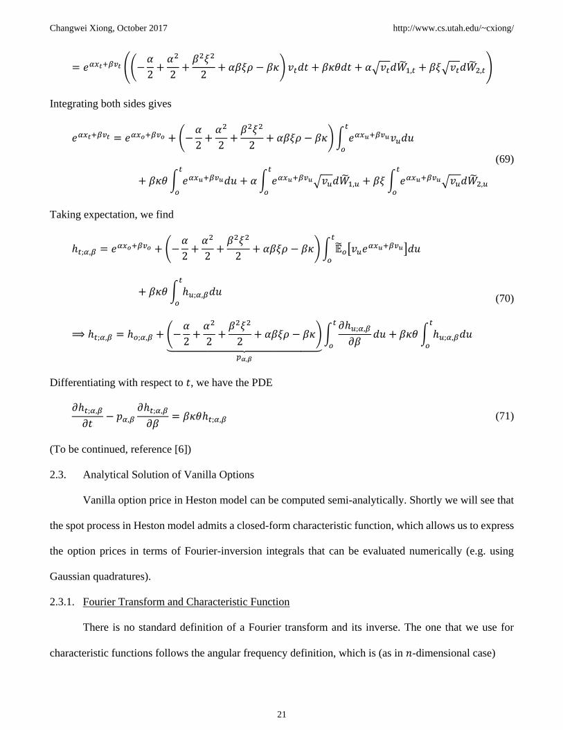
𝜕𝛽= 𝛽𝜅𝜃ℎ𝑡;𝛼,𝛽 (71)
(To be continued, reference [6])
2.3. Analytical Solution of Vanilla Options
Vanilla option price in Heston model can be computed semi-analytically. Shortly we will see that
the spot process in Heston model admits a closed-form characteristic function, which allows us to express
the option prices in terms of Fourier-inversion integrals that can be evaluated numerically (e.g. using
Gaussian quadratures).
2.3.1. Fourier Transform and Characteristic Function
There is no standard definition of a Fourier transform and its inverse. The one that we use for
characteristic functions follows the angular frequency definition, which is (as in 𝑛-dimensional case)

Changwei Xiong, October 2017 http://www.cs.utah.edu/~cxiong/
22
Forward: 𝑓𝜔 = ∫ 𝑒𝑖𝜔′𝑥𝑓𝑥𝑑𝑥
ℝ𝑛 ∀ 𝜔 ∈ ℝ𝑛
Inverse: 𝑓𝑥 =1
(2𝜋)𝑛∫ 𝑒−𝑖𝜔
′𝑥𝑓𝜔𝑑𝜔ℝ𝑛
∀ 𝑥 ∈ ℝ𝑛
(72)
where the 𝜔 is the angular frequency and the (′) denotes matrix transpose (the dot product of two column
vectors 𝜔 and 𝑥). In fact the normalization factors multiplying the forward and inverse transforms (here
1 and 1/(2𝜋)𝑛, respectively) and the signs of the exponents are merely conventions and differ in some
treatments. The only requirements of these conventions are: 1. the forward and inverse transforms have
opposite-sign exponents, and 2. the product of their normalization factors is 1/(2𝜋)𝑛. In one-dimension,
the (72) reduces to
Forward: 𝑓𝜔 = ∫𝑒𝑖𝜔𝑥𝑓𝑥𝑑𝑥
ℝ
∀ 𝜔 ∈ ℝ
Inverse: 𝑓𝑥 =1
2𝜋∫𝑒−𝑖𝜔𝑥𝑓𝜔𝑑𝜔ℝ
∀ 𝑥 ∈ ℝ
(73)
The transform is equivalent to the case we write a periodic function 𝑓𝑥 with period 2𝜋/ℎ in terms of
Fourier series expansion
𝑓𝑥 =ℎ
2𝜋∑ 𝑐ℎ𝑘
∞
𝑘=−∞
𝑒−𝑖ℎ𝑘𝑥 where 𝑐ℎ𝑘 = ∫ 𝑓𝑥𝑒𝑖ℎ𝑘𝑥𝑑𝑥
𝜋/ℎ
−𝜋/ℎ
∀ ℎ > 0 (74)
Taking the limit ℎ → 0+, we have
limℎ→0+
𝑐ℎ𝑘 = limℎ→0+
∫ 𝑓𝑥𝑒𝑖ℎ𝑘𝑥𝑑𝑥
𝜋ℎ
−𝜋ℎ
= ∫ 𝑓𝑥𝑒𝑖𝜔𝑥𝑑𝑥
ℝ
= 𝑓𝜔 and
𝑓𝑥 = limℎ→0+
ℎ
2𝜋∑ 𝑐ℎ𝑘𝑒
−𝑖ℎ𝑘𝑥
∞
𝑘=−∞
=1
2𝜋∫ 𝑓𝜔𝑒
−𝑖𝜔𝑥𝑑𝜔ℝ
where 𝜔 = ℎ𝑘
(75)
The sum can be regarded as an approximating Riemann sum for the integral [7].
Characteristic function 𝜙𝜔 of any random variable 𝑋 complete defines its probability distribution.
On the real line the characteristic function is given by the following formula

Changwei Xiong, October 2017 http://www.cs.utah.edu/~cxiong/
23
𝜙𝜔 ≡ 𝔼[𝑒𝑖𝜔𝑋] = ∫𝑒𝑖𝜔𝑥𝑝𝑥𝑑𝑥
ℝ
= ∫𝑒𝑖𝜔𝑥𝑑𝑃𝑥Ω
∀ 𝜔 ∈ ℝ (76)
where the 𝑝𝑥 denotes the probability density function (PDF) and the 𝑃𝑥 = ∫ 𝑝𝑦𝑑𝑦𝑥
−∞ is the cumulative
density function (CDF). The characteristic function is merely a Fourier transform of the 𝑝𝑥, likewise the
𝑝𝑥 can be recovered from 𝜙𝜔 through the inverse Fourier transform [8]
𝑝𝑥 =1
2𝜋∫𝑒−𝑖𝜔𝑥𝜙𝜔𝑑𝜔ℝ
∀ 𝜔 ∈ ℝ (77)
The 𝑃𝑥 can be computed from 𝜙𝜔 through Levy’s Inversion Formula [9] [10] [11]
𝑃𝑥 =𝜙02+1
2𝜋∫
𝑒𝑖𝜔𝑥𝜙−𝜔 − 𝑒−𝑖𝜔𝑥𝜙𝜔
𝑖𝜔𝑑𝜔
ℝ+
(78)
where 𝜙0 = 1 if 𝜙𝜔 is a characteristic function of a random variable. Before proving the formula, we need
to find Fourier transform of signum function 𝒮𝑥, which is defined as
𝒮𝑥 = {−1 if 𝑥 < 01 if 𝑥 > 0
(79)
Its transform cannot be obtained via direct integration. However we can consider an odd two-sided
exponential function 𝒮𝑥ℎ with ℎ > 0
𝒮𝑥ℎ = {−𝑒
ℎ𝑥 if 𝑥 < 0𝑒−ℎ𝑥 if 𝑥 > 0
(80)
The �̂�𝜔ℎ, i.e. the Fourier transform of 𝒮𝑥
ℎ, can then be derived as
�̂�𝜔ℎ = ∫𝑒𝑖𝜔𝑥𝒮𝑥
ℎ𝑑𝑥ℝ
= −∫ 𝑒(𝑖𝜔+ℎ)𝑥𝑑𝑥ℝ−
+∫ 𝑒(𝑖𝜔−ℎ)𝑥𝑑𝑥ℝ+
= −𝑒(𝑖𝜔+ℎ)𝑥
𝑖𝜔 + ℎ|𝑥=−∞
0
+𝑒(𝑖𝜔−ℎ)𝑥
𝑖𝜔 − ℎ|𝑥=0
∞
= −1
𝑖𝜔 + ℎ−
1
𝑖𝜔 − ℎ=
2𝑖𝜔
𝜔2 + ℎ2
(81)
The parameter ℎ controls how rapidly the exponential function decays. As we let ℎ → 0, the exponential
function resembles more and more closely the signum function. This suggests that
�̂�𝜔 = limℎ→0
�̂�𝜔ℎ = lim
ℎ→0
2𝑖𝜔
𝜔2 + ℎ2= −
2
𝑖𝜔 (82)
Hence the inverse transform of the �̂�𝜔 gives

Changwei Xiong, October 2017 http://www.cs.utah.edu/~cxiong/
24
𝒮𝑥 =1
2𝜋∫𝑒−𝑖𝜔𝑥�̂�𝜔𝑑𝜔ℝ
= −1
𝜋∫𝑒−𝑖𝜔𝑥
𝑖𝜔𝑑𝜔
ℝ
= −1
𝜋∫cos𝜔𝑥 − 𝑖 sin𝜔𝑥
𝑖𝜔𝑑𝜔
ℝ
= −1
𝑖𝜋∫cos𝜔𝑥
𝜔𝑑𝜔
ℝ⏟ =0, (odd function)
+1
𝜋∫sin𝜔𝑥
𝜔𝑑𝜔
ℝ
=2
𝜋∫
sin𝜔𝑥
𝜔𝑑𝜔
ℝ+
(83)
With the help of the signum function 𝒮𝑥 in (83), the proof of (78) is given as follows
∫𝑒𝑖𝜔𝑥𝜙−𝜔 − 𝑒
−𝑖𝜔𝑥𝜙𝜔𝑖𝜔
𝑑𝜔ℝ+
= ∫𝑒𝑖𝜔𝑥 ∫ 𝑒−𝑖𝜔𝑦𝑝𝑦𝑑𝑦ℝ
− 𝑒−𝑖𝜔𝑥 ∫ 𝑒𝑖𝜔𝑦𝑝𝑦𝑑𝑦ℝ
𝑖𝜔𝑑𝜔
ℝ+
= ∫ ∫𝑒𝑖𝜔(𝑥−𝑦) − 𝑒−𝑖𝜔(𝑥−𝑦)
𝑖𝜔𝑝𝑦𝑑𝑦
ℝ
𝑑𝜔ℝ+
= ∫ ∫𝑒𝑖𝜔(𝑥−𝑦) − 𝑒−𝑖𝜔(𝑥−𝑦)
𝑖𝜔𝑑𝜔
ℝ+
𝑝𝑦𝑑𝑦ℝ
(by Fubini′s theorem)
= 2∫ ∫sin𝜔(𝑥 − 𝑦)
𝜔𝑑𝜔
ℝ+
𝑝𝑦𝑑𝑦ℝ
(by 𝑒𝑖𝑥 = cos 𝑥 + 𝑖 sin 𝑥)
= 𝜋∫𝒮𝑥−𝑦𝑝𝑦𝑑𝑦ℝ
= 𝜋 (−∫ 𝑝𝑦𝑑𝑦∞
𝑥
+∫ 𝑝𝑦𝑑𝑦𝑥
−∞
) = 𝜋 (−∫𝑝𝑦𝑑𝑦ℝ
+ 2∫ 𝑝𝑦𝑑𝑦𝑥
−∞
)
= 𝜋(−𝜙0 + 2𝑃𝑥)
(84)
The Levy Inversion Formula can also be written in the following form
𝑃𝑥 =𝜙02−1
2𝜋∫𝑒−𝑖𝜔𝑥𝜙𝜔𝑖𝜔
𝑑𝜔ℝ
(85)
which can be proved as
∫𝑒−𝑖𝜔𝑥𝜙𝜔𝑖𝜔
𝑑𝜔ℝ
= ∫𝑒−𝑖𝜔𝑥 ∫ 𝑒𝑖𝜔𝑦𝑝𝑦𝑑𝑦ℝ
𝑖𝜔𝑑𝜔
ℝ
= ∫ ∫𝑒𝑖𝜔(𝑦−𝑥)
𝑖𝜔𝑝𝑦𝑑𝑦
ℝ
𝑑𝜔ℝ
= ∫ ∫𝑒𝑖𝜔(𝑦−𝑥)
𝑖𝜔𝑑𝜔
ℝ
𝑝𝑦𝑑𝑦ℝ
= 𝜋∫𝒮𝑥−𝑦𝑝𝑦𝑑𝑦ℝ
= 𝜋(−𝜙0 + 2𝑃𝑥)
where ∫𝑒𝑖𝜔𝑥
𝑖𝜔𝑑𝜔
ℝ
= ∫𝑒𝑖𝜔𝑥
𝑖𝜔𝑑𝜔
ℝ−
+∫𝑒𝑖𝜔𝑥
𝑖𝜔𝑑𝜔
ℝ+
= ∫𝑒−𝑖𝜔𝑥
−𝑖𝜔𝑑𝜔
ℝ+
+∫𝑒𝑖𝜔𝑥
𝑖𝜔𝑑𝜔
ℝ+
= ∫𝑒𝑖𝜔𝑥 − 𝑒−𝑖𝜔𝑥
𝑖𝜔𝑑𝜔
ℝ+
= 2∫sin𝜔𝑥
𝜔𝑑𝜔
ℝ+= 𝜋𝒮𝑥
(86)

Changwei Xiong, October 2017 http://www.cs.utah.edu/~cxiong/
25
Note that if 𝑝𝑥 is real-valued function (i.e. probability density function), its Fourier transform 𝜙𝜔
is then even in its real part and odd in its imaginary part [12], we therefore have 𝜙𝜔 = 𝜙−𝜔̅̅ ̅̅ ̅̅ , the inversion
formula (85) becomes identical to (78), which can be further reduced to
𝑃𝑥 =𝜙02+1
2𝜋∫
𝑒𝑖𝜔𝑥𝜙−𝜔 − 𝑒−𝑖𝜔𝑥𝜙𝜔
𝑖𝜔𝑑𝜔
ℝ+
=𝜙02+1
2𝜋∫
𝑒−𝑖𝜔𝑥𝜙𝜔̅̅ ̅̅ ̅̅ ̅̅ ̅̅ ̅ − 𝑒−𝑖𝜔𝑥𝜙𝜔𝑖𝜔
𝑑𝜔ℝ+
=𝜙02−1
𝜋∫ ℜ[
𝑒−𝑖𝜔𝑥𝜙𝜔𝑖𝜔
] 𝑑𝜔ℝ+
=𝜙02−1
𝜋∫ ℑ [
𝑒−𝑖𝜔𝑥𝜙𝜔𝜔
]𝑑𝜔ℝ+
(87)
For 𝑃𝑥𝐶 = ∫ 𝑝𝑦𝑑𝑦
∞
𝑥, the complementary of 𝑃𝑥, we can use the simple relation 𝑃𝑥
𝐶 = 𝜙0 − 𝑃𝑥
𝑃𝑥𝐶 =
𝜙02−1
2𝜋∫
𝑒𝑖𝜔𝑥𝜙−𝜔 − 𝑒−𝑖𝜔𝑥𝜙𝜔
𝑖𝜔𝑑𝜔
ℝ+
=𝜙02+1
𝜋∫ ℜ[
𝑒−𝑖𝜔𝑥𝜙𝜔𝑖𝜔
] 𝑑𝜔ℝ+
=𝜙02+1
𝜋∫ ℑ [
𝑒−𝑖𝜔𝑥𝜙𝜔𝜔
]𝑑𝜔ℝ+
(88)
2.3.2. Characteristic Function
In this section, we present a derivation of the closed form characteristic function of the spot in
Heston model [13]. The definition of the Heston joint process in (48) will be used. Suppose there exists a
payoff function 𝑔𝑥𝑇,𝑣𝑇 on 𝑥𝑇 and 𝑣𝑇, we may calculate risk neutral expectation of the payoff function as
ℎ𝑡 = �̃�𝑡[𝑔𝑥𝑇,𝑣𝑇] (89)
For example, the characteristic function of the joint distribution of 𝑥𝑇 and 𝑣𝑇 would be given by
𝜙𝑡;𝛼,𝛽 = �̃�𝑡[𝑔𝑥𝑇,𝑣𝑇;𝛼,𝛽] where 𝑔𝑥𝑇,𝑣𝑇;𝛼,𝛽 = exp(𝑖𝛼𝑥𝑇 + 𝑖𝛽𝑣𝑇) (90)
The risk neutral expectation is actually a martingale because for 𝑜 < 𝑡 < 𝑇
ℎ𝑜 = �̃�𝑜[𝑔𝑥𝑇,𝑣𝑇] = �̃�𝑜 [�̃�𝑡[𝑔𝑥𝑇,𝑣𝑇]] = �̃�𝑜[ℎ𝑡] (91)
Applying Ito’s lemma to ℎ and forcing the drift to be zero (martingale property), we end up with a PDE
𝜕ℎ
𝜕𝑡−𝑣
2
𝜕ℎ
𝜕𝑥+ 𝜅(𝜃 − 𝑣)
𝜕ℎ
𝜕𝑣+𝑣
2
𝜕2ℎ
𝜕𝑥2+𝜉2𝑣
2
𝜕2ℎ
𝜕𝑣2+ 𝜉𝜌𝑣
𝜕2ℎ
𝜕𝑥𝜕𝑣= 0 (92)

Changwei Xiong, October 2017 http://www.cs.utah.edu/~cxiong/
26
To determine the solution of (92), the terminal condition ℎ𝑇 = �̃�𝑇[𝑔𝑥𝑇,𝑣𝑇] = 𝑔𝑥𝑇,𝑣𝑇 at time 𝑇 must be
specified. The terminal payoff function that we will consider has the form 𝑔𝑥𝑇,𝑣𝑇 = 𝑒𝛾+𝛿𝑣𝑇+𝑖𝛼𝑥𝑇. If 𝛾 = 0
and 𝛿 = 𝑖𝛽, the resulting payoff function becomes 𝑔𝑥𝑇,𝑣𝑇;𝛼,𝛽 in (90), corresponding to the characteristic
function of the joint distribution.
Heston [22] guessed a solution that has the form
ℎ𝑡 = �̃�𝑡[𝑔𝑥𝑇,𝑣𝑇] = 𝑒𝐶+𝐷𝑣𝑡+𝑖𝛼𝑥𝑡 where 𝐶 = 𝐶𝜏,𝛼,𝛾,𝛿 , 𝐷 = 𝐷𝜏,𝛼,𝛾,𝛿 , 𝜏 = 𝑇 − 𝑡 (93)
Substituting the tentative solution (93) in (92) yields
𝜕𝐶
𝜕𝑡+ 𝑣
𝜕𝐷
𝜕𝑡−𝑖𝛼𝑣
2+ 𝜅(𝜃 − 𝑣)𝐷 −
𝛼2𝑣
2+𝜉2𝑣
2𝐷2 + 𝑖𝛼𝐷𝜉𝜌𝑣 = 0
⟹𝜕𝐶
𝜕𝑡+ 𝜅𝜃𝐷 + (
𝜕𝐷
𝜕𝑡+𝜉2
2𝐷2 −𝑚𝐷 −−
𝛼(𝑖 + 𝛼)
2) 𝑣 = 0 where 𝑚 = 𝜅 − 𝛼𝜉𝜌𝑖
(94)
As the 𝑣 is an independent variable, (94) is zero only if
𝜕𝐶
𝜕𝑡+ 𝜅𝜃𝐷 = 0 and
𝜕𝐷
𝜕𝑡+𝜉2
2𝐷2 −𝑚𝐷 −
𝛼(𝑖 + 𝛼)
2= 0 (95)
Changing the variable 𝑡 to 𝜏 = 𝑇 − 𝑡, we have
𝜕𝐶
𝜕𝜏− 𝜅𝜃𝐷 = 0 and
𝜕𝐷
𝜕𝜏−𝜉2
2𝐷2 +𝑚𝐷 +
𝛼(𝑖 + 𝛼)
2= 0 (96)
The terminal condition for this system of equations is given by 𝐶𝜏=0 = 𝛾 and 𝐷𝜏=0 = 𝛿. The ODE for 𝐷
is a Riccati equation that only depends on 𝐷. This Riccati equation can be turned into an ODE through the
change of variable, 𝑍 = (𝐷 − �̂�)−1
, where �̂� is a particular solution to the second equation in (96)
𝜕𝑍
𝜕𝜏= −
1
(𝐷 − �̂�)2
𝜕(𝐷 − �̂�)
𝜕𝜏= −𝑍2 (
𝜉2
2𝐷2 −𝑚𝐷 −
𝜉2
2�̂�2 +𝑚�̂�)
= −𝑍 (𝜉2
2(𝐷 + �̂�) − 𝑚) = −𝑍 (
𝜉2
2(𝐷 − �̂� + 2�̂�)) + 𝑚𝑍 = −(𝜉2�̂� − 𝑚)𝑍 −
𝜉2
2
⟹𝜕𝑍
𝜕𝜏+ (𝜉2�̂� − 𝑚)𝑍 +
𝜉2
2= 0 or
(97)

Changwei Xiong, October 2017 http://www.cs.utah.edu/~cxiong/
27
𝜕𝑍
𝜕𝜏+ 𝐵𝑍 + 𝐴 = 0 where 𝐴 =
𝜉2
2, 𝐵 = 𝜉2�̂� − 𝑚
The solution to (97) is given by
𝑍 = −𝐴
𝐵 + (𝑍0 +
𝐴
𝐵 ) 𝑒−𝐵𝜏 where 𝑍0 =
1
𝐷0 − �̂�=
1
𝛿 − �̂�
⟹𝐷 =1
−𝐴𝐵 + (𝑍0 +
𝐴𝐵 ) 𝑒−𝐵𝜏
+ �̂�
(98)
The particular solution �̂� can be as simple as a constant, which implies it would be the solution of the
quadratic equation
−𝜉2
2�̂�2 +𝑚�̂� +
𝛼(𝑖 + 𝛼)
2= 0 ⟹ �̂� =
𝑚 + 𝑑
𝜉2 where 𝑑 = ±√𝑚2 + 𝜉2𝛼(𝑖 + 𝛼) (99)
This particular solution for �̂� makes 𝐵 = 𝑑. The solution for 𝐷 in (98) can then be derived
𝐷 =1
−𝜉2
2𝑑+ (
−𝜉2
𝑚+ 𝑑 − 𝛿𝜉2+𝜉2
2𝑑) 𝑒−𝑑𝜏
+𝑚 + 𝑑
𝜉2
⟹ 𝜉2𝐷 = −2𝑑(𝑚 + 𝑑 − 𝛿𝜉2)
2𝑒−𝑑𝜏𝑑 + (𝑚 + 𝑑 − 𝛿𝜉2)(1 − 𝑒−𝑑𝜏)+ 𝑚 + 𝑑
= −2𝑑(𝑚 + 𝑑 − 𝛿𝜉2)
(𝑚 + 𝑑 − 𝛿𝜉2) − (𝑚 − 𝑑 − 𝛿𝜉2)𝑒−𝑑𝜏+𝑚 + 𝑑
= −2𝑑
1 − �̂�𝑒−𝑑𝜏+𝑚 + 𝑑 (by defining �̂� =
𝑚 − 𝑑 − 𝛿𝜉2
𝑚+ 𝑑 − 𝛿𝜉2)
=(𝑚 + 𝑑)(1 − �̂�𝑒−𝑑𝜏) − 2𝑑
1 − �̂�𝑒−𝑑𝜏=𝑚 − 𝑑 − (𝑚 + 𝑑)�̂�𝑒−𝑑𝜏
1 − �̂�𝑒−𝑑𝜏
= (𝑚 + 𝑑)𝑔 − �̂�𝑒−𝑑𝜏
1 − �̂�𝑒−𝑑𝜏 (by defining 𝑔 =
𝑚 − 𝑑
𝑚 + 𝑑)
⟹𝐷 =𝑚 + 𝑑
𝜉2𝑔 − �̂�𝑒−𝑑𝜏
1 − �̂�𝑒−𝑑𝜏
(100)
The 𝐷 can then be plugged into the ODE for 𝐶 in (96)

Changwei Xiong, October 2017 http://www.cs.utah.edu/~cxiong/
28
𝜕𝐶
𝜕𝜏− 𝜅𝜃
𝑚 + 𝑑
𝜉2𝑔 − �̂�𝑒−𝑑𝜏
1 − �̂�𝑒−𝑑𝜏= 0 ⟹ 𝐶 = 𝜅𝜃
𝑚 + 𝑑
𝜉2∫𝑔 − �̂�𝑒−𝑑𝜏
1 − �̂�𝑒−𝑑𝜏𝑑𝜏 + 𝐾𝐶 (101)
where 𝐾𝐶 is a constant to be fixed by terminal condition. The indefinite integral in (101) can be solved
through change of variable 𝑢 = 𝑒−𝑑𝜏 where 𝜕𝑢
𝜕𝜏= −𝑢𝑑
∫𝑔 − �̂�𝑒−𝑑𝜏
1 − �̂�𝑒−𝑑𝜏𝜕𝜏 = −∫(
𝑔 − �̂�𝑢
1 − �̂�𝑢)1
𝑢𝑑𝜕𝑢 = −
1
𝑑∫(
𝑔𝑢 − �̂�
1 − �̂�𝑢)𝜕𝑢
= −1
𝑑∫(
𝑔𝑢 − �̂� −
𝑔𝑢(1 − �̂�𝑢)
1 − �̂�𝑢+𝑔
𝑢)𝜕𝑢 = −
1
𝑑∫(
(𝑔 − 1)�̂�
1 − �̂�𝑢+𝑔
𝑢)𝜕𝑢
=𝑔 − 1
𝑑ln(1 − �̂�𝑢) −
𝑔
𝑑ln 𝑢 =
𝑔 − 1
𝑑ln(1 − �̂�𝑒−𝑑𝜏) + 𝑔𝜏
(102)
which gives
𝐶 = 𝜅𝜃𝑚 + 𝑑
𝜉2(𝑔 − 1
𝑑ln(1 − �̂�𝑒−𝑑𝜏) + 𝑔𝜏) + 𝐾𝐶
=𝜅𝜃
𝜉2(−2 ln(1 − �̂�𝑒−𝑑𝜏) + (𝑚 − 𝑑)𝜏) + 𝐾𝐶
(103)
We then fix 𝐾𝐶 by 𝐶0 = 𝛾
𝐶0 = −2𝜅𝜃
𝜉2ln(1 − �̂�) + 𝐾𝐶 = 𝛾 ⟹ 𝐾𝐶 = 2
𝜅𝜃
𝜉2ln(1 − �̂�) + 𝛾 (104)
Therefore we have the solution for 𝐶
𝐶 =𝜅𝜃
𝜉2(2 ln
1 − �̂�
1 − �̂�𝑒−𝑑𝜏 + (𝑚 − 𝑑)𝜏) + 𝛾 (105)
Combining the solutions in (100) and (105), the ℎ𝑡 is of the following form
ℎ𝑡 = �̃�𝑡[𝑔𝑥𝑇,𝑣𝑇] = exp(𝐶 + 𝐷𝑣𝑡 + 𝑖𝛼𝑥𝑡) where
𝑚 = 𝜅 − 𝛼𝜉𝜌𝑖, 𝑑 = ±√𝑚2 + 𝜉2𝛼(𝑖 + 𝛼), 𝑔 =𝑚 − 𝑑
𝑚 + 𝑑, �̂� =
𝑚 − 𝑑 − 𝛿𝜉2
𝑚+ 𝑑 − 𝛿𝜉2
𝐶 =𝜅𝜃
𝜉2(2 ln
1 − �̂�
1 − �̂�𝑒−𝑑𝜏 + (𝑚 − 𝑑)𝜏) + 𝛾, 𝐷 =
𝑚 + 𝑑
𝜉2𝑔 − �̂�𝑒−𝑑𝜏
1 − �̂�𝑒−𝑑𝜏
(106)

Changwei Xiong, October 2017 http://www.cs.utah.edu/~cxiong/
29
The marginal characteristic function of 𝑥𝑇 is given by 𝛾 = 0 and 𝛿 = 0 where �̂� = 𝑔
𝜙𝛼𝑥𝑇 = exp(
𝜅𝜃
𝜉2(2 ln
1 − 𝑔
1 − 𝑔𝑒−𝑑𝜏+ (𝑚 − 𝑑)𝜏) +
𝑚 − 𝑑
𝜉21 − 𝑒−𝑑𝜏
1 − 𝑔𝑒−𝑑𝜏𝑣𝑡 + 𝑖𝛼𝑥𝑡)
where 𝑚 = 𝜅 − 𝛼𝜉𝜌𝑖, 𝑑 = ±√𝑚2 + 𝜉2𝛼(𝑖 + 𝛼), 𝑔 =𝑚 − 𝑑
𝑚 + 𝑑
(107)
2.3.3. Vanilla Option Prices
Once we know the analytical form of the characteristic function 𝜙𝛼𝑥𝑇 of the centered log-spot 𝑥𝑇,
we are able to compute the vanilla option prices using inversion methods. Here, we are going to discuss
two methods, which treat the option price function analogous to the cumulative density function or the
probability density function, respectively. In addition, we also summarize the original Heston’s method
[22].
2.3.3.1. Analogy to Cumulative Density Function
For 𝑡 ≤ 𝑇, using a European call option as an example we change the variable to 𝑥𝑡 as in (47)
𝐶𝑇,𝐾 = �̃�𝑡 [𝑀𝑡𝑀𝑇
(𝑆𝑇 − 𝐾)+] = 𝑒−𝑟𝜏𝐹𝑡,𝑇�̃�𝑡[(𝑒
𝑥𝑇 − 𝑒𝒦)+]
with 𝜏 = 𝑇 − 𝑡, 𝜇 = 𝑟 − 𝑞, 𝐹𝑡,𝑇 = 𝑆𝑡𝑒𝜇𝜏, 𝑥𝑇 = ln
𝑆𝑇𝐹𝑡,𝑇
, 𝒦 = ln𝐾
𝐹𝑡,𝑇
(108)
where the cash account 𝑀𝑇 = 𝑀𝑡 exp (∫ 𝑟𝑢𝑑𝑢𝑇
𝑡) and the interest rate 𝑟 and dividend yield 𝑞 are assumed
constant. We then define an option forward price in percentage of the underlying forward as a function of
moneyness 𝒦 defined as the log strike over forward
𝒞𝒦 =𝐶𝑇,𝐾
𝑒−𝑟𝜏𝐹𝑡,𝑇= �̃�𝑡[(𝑒
𝑥𝑇 − 𝑒𝒦)+] = �̃�𝑡[(𝑒𝑥𝑇 − 𝑒𝒦)𝟙{𝑥𝑇 > 𝒦}]
where 𝟙{𝑥 > 𝑋} = {1 if 𝑥 > 𝑋0 otherwise
(109)
Given we know the characteristic function of the log-spot process 𝑥𝑇, we can derive the Fourier transform
of the call option, then use numerical inversion to obtain option prices directly [14]. Since 𝐶𝑇,𝐾 ∈

Changwei Xiong, October 2017 http://www.cs.utah.edu/~cxiong/
30
[0, 𝑒−𝑟𝜏𝐹𝑜,𝑇], we have 𝒞𝒦 ∈ [0,1], which can treated as a cumulative density function on 𝒦, the Fourier
transform of the option price is then given by
𝜒𝜔𝑐 = ∫ 𝑒𝑖𝜔𝒦𝑑𝒞𝒦
𝒦∈ℝ
= 𝑒𝑖𝜔𝒦𝒞𝒦|𝒦=−∞∞
−∫𝑖𝜔𝑒𝑖𝜔𝒦𝒞𝒦𝑑𝒦ℝ
= −𝑒−𝑖𝜔∞ −∫𝑖𝜔𝑒𝑖𝜔𝒦𝒞𝒦𝑑𝒦ℝ
(by 𝒞∞ = 0 and 𝒞−∞ = 1)
= −𝑒−𝑖𝜔∞ −∫ 𝑖𝜔𝑒𝑖𝜔𝒦∫(𝑒𝑥 − 𝑒𝒦)𝟙{𝑥 > 𝒦}𝑑𝑃𝑥𝑥𝑇
Ω
𝑑𝒦ℝ
= −𝑒−𝑖𝜔∞ −∫ ∫𝑖𝜔(𝑒𝑖𝜔𝒦+𝑥 − 𝑒(𝑖𝜔+1)𝒦)𝟙{𝑥 > 𝒦}𝑑𝒦ℝ
𝑑𝑃𝑥𝑥𝑇
Ω
(by Fubini′s theorem)
= −𝑒−𝑖𝜔∞ −∫ ∫ 𝑖𝜔(𝑒𝑖𝜔𝒦+𝑥 − 𝑒(𝑖𝜔+1)𝒦)𝑑𝒦𝑥
−∞
𝑑𝑃𝑥𝑥𝑇
Ω
= −𝑒−𝑖𝜔∞ −∫ (𝑒𝑖𝜔𝒦+𝑥 −𝑖𝜔𝑒(𝑖𝜔+1)𝒦
𝑖𝜔 + 1)|𝒦=−∞
𝑥
𝑑𝑃𝑥𝑥𝑇
Ω
= −𝑒−𝑖𝜔∞ −∫ (𝑒(𝑖𝜔+1)𝑥 − 𝑒−𝑖𝜔∞+𝑥 −𝑖𝜔𝑒(𝑖𝜔+1)𝑥
𝑖𝜔 + 1+𝑖𝜔𝑒−(𝑖𝜔+1)∞
𝑖𝜔 + 1⏟ =0
)𝑑𝑃𝑥𝑥𝑇
Ω
= −𝑒−𝑖𝜔∞ + 𝑒−𝑖𝜔∞∫𝑒𝑥𝑑𝑃𝑥𝑥𝑇
Ω
−∫ (𝑒(𝑖𝜔+1)𝑥 −𝑖𝜔𝑒(𝑖𝜔+1)𝑥
𝑖𝜔 + 1)𝑑𝑃𝑥
Ω
= −1
𝑖𝜔 + 1∫𝑒𝑖(𝜔−i)𝑥𝑑𝑃𝑥
𝑥𝑇
Ω
(by ∫ 𝑒𝑥𝑑𝑃𝑥𝑥𝑇
Ω
=1
𝐹𝑇�̃�0[𝑆𝑇] = 1)
= −𝜙𝜔−𝑖𝑥𝑇
𝑖𝜔 + 1
(110)
The 𝜒𝜔𝑐 is the characteristic function of the option forward price 𝒞𝒦, which is treated just as a cumulative
density function. The price is then given by the Levy’s Inversion Formula (78) [15]
𝒞𝒦 =𝜒02+1
2𝜋∫
𝑒𝑖𝜔𝒦𝜒−𝜔𝑐 − 𝑒−𝑖𝜔𝒦𝜒𝜔
𝑐
𝑖𝜔𝑑𝜔
ℝ+
(111)

Changwei Xiong, October 2017 http://www.cs.utah.edu/~cxiong/
31
=1
2+1
2𝜋∫
𝑒𝑖𝜔𝒦𝜙−𝜔−𝑖𝑥𝑇
𝑖𝜔 − 1 + 𝑒−𝑖𝜔𝒦 𝜙𝜔−𝑖
𝑥𝑇
𝑖𝜔 + 1𝑖𝜔
𝑑𝜔ℝ+
(by 𝜒0𝑐 = −𝜙−𝑖 = 1)
=1
2+1
2𝜋∫ (𝑒𝑖𝜔𝒦
𝜙−𝜔−𝑖𝑥𝑇
−𝜔2 − 𝑖𝜔+ 𝑒−𝑖𝜔𝒦
𝜙𝜔−𝑖𝑥𝑇
−𝜔2 + 𝑖𝜔)𝑑𝜔
ℝ+
=1
2−1
2𝜋∫ (𝑒𝑖𝜔𝒦
𝜙−𝜔−𝑖𝑥𝑇
𝜔2 + 𝑖𝜔+ 𝑒−𝑖𝜔𝒦
𝜙𝜔−𝑖𝑥𝑇
𝜔2 − 𝑖𝜔)𝑑𝜔
ℝ+
In the integrand of (111), the 𝜙𝑢𝜔−𝑖𝑥𝑇 for 𝑢 = ±1 can be derived from the characteristic function 𝜙𝛼
𝑥𝑇 in
(107) and given as follows (note that 𝑥𝑡 = 0)
𝜙𝑢𝜔−𝑖𝑥𝑇 = exp(
𝜅𝜃
𝜉2(2 ln
1 − 𝑔
1 − 𝑔𝑒−𝑑𝜏+ (𝑚 − 𝑑)𝜏) +
𝑚 − 𝑑
𝜉21 − 𝑒−𝑑𝜏
1 − 𝑔𝑒−𝑑𝜏𝑣𝑡)
with 𝜏 = 𝑇 − 𝑡, 𝑚 = 𝜅 − 𝑢𝜔𝜉𝜌𝑖 − 𝜉𝜌, 𝑑 = ±√𝑚2 + 𝜉2𝜔(𝜔 − 𝑢𝑖), 𝑔 =𝑚 − 𝑑
𝑚 + 𝑑
(112)
The inversion formula in (111) involves evaluation of the 𝜙𝑢𝜔−𝑖𝑥𝑇 function twice, which is less efficient.
Since 𝒞𝒦 is real-valued, we may use (87) to perform the inversion
𝒞𝒦 =𝜒02−1
𝜋∫ ℑ [
𝑒−𝑖𝜔𝒦𝜒𝜔𝑐
𝜔]
ℝ+
=1
2+1
𝜋∫ ℑ [𝑒−𝑖𝜔𝒦
𝜙𝜔−𝑖𝑥𝑇
𝑖𝜔2 +ω]𝑑𝜔
ℝ+
(113)
where 𝜙𝜔−𝑖𝑥𝑇 is given in (112) with 𝑢 = 1 and the integral can be estimated numerically by Gauss-
Laguerre quadrature. Once we have 𝒞𝒦 for log-moneyness, the call option price can be computed by (109)
𝐶𝑇,𝐾 = 𝒞𝒦𝑒−𝑟𝜏𝑆𝑡𝑒
𝜇𝜏 = 𝒞𝒦𝑆𝑡𝑒−𝑞𝜏 (114)
and the put option price by call-put parity
𝐶𝑇,𝐾 − 𝑃𝑇,𝐾 = 𝑒−𝑟𝜏(𝐹𝑡,𝑇 − 𝐾) ⟹ 𝑃𝑇,𝐾 = 𝐶𝑇,𝐾 − 𝑆𝑡𝑒
−𝑞𝜏 + 𝑒−𝑟𝜏𝐾 (115)
2.3.3.2. Analogy to Probability Density Function
In this section, we treat 𝒞𝒦 analogous to a probability density [16] [17] and define in terms of
generalized Fourier transform with 𝑧 = 𝑧𝑟 − 𝑖𝑧𝑖 , 𝑧𝑟 ∈ ℝ, 𝑧𝑖 ∈ 𝒟 ⊆ ℝ+
𝜒𝑧𝑝= ∫𝑒𝑖𝑧𝒦𝒞𝒦𝑑𝒦
ℝ
= ∫𝑒𝑖𝑧𝒦�̃�𝑡[(𝑒𝑥𝑇 − 𝑒𝒦)𝟙{𝑥𝑇 > 𝒦}]𝑑𝒦
ℝ
(116)

Changwei Xiong, October 2017 http://www.cs.utah.edu/~cxiong/
32
= �̃�𝑡 [∫𝑒𝑖𝑧𝒦(𝑒𝑥𝑇 − 𝑒𝒦)𝟙{𝑥𝑇 > 𝒦}𝑑𝒦
ℝ
] = �̃�𝑡 [∫ 𝑒𝑖𝑧𝒦(𝑒𝑥𝑇 − 𝑒𝒦)𝑑𝒦𝑥𝑇
−∞
]
= �̃�𝑡 [(𝑒𝑖𝑧𝒦+𝑥𝑇
𝑖𝑧−𝑒(𝑖𝑧+1)𝒦
𝑖𝑧 + 1)|𝒦=−∞
𝑥𝑇
] = �̃�𝑡 [𝑒(𝑖𝑧+1)𝑥𝑇
𝑖𝑧 − 𝑧2] (by lim
𝒦→−∞𝑒𝑖𝑧𝒦 = 0)
= �̃�𝑡 [𝑒𝑖(𝑧−𝑖)𝑥𝑇
𝑖𝑧 − 𝑧2] =
𝜙𝑧−𝑖𝑥𝑇
𝑖𝑧 − 𝑧2
For some return distributions, the return transform 𝜙𝑧−𝑖𝑥𝑇 is well-defined only when 𝑧𝑖 is in a subset of the
real line. We use 𝒟 ⊆ ℝ+ to denote the subset that both guarantees the convergence of 𝑒𝑖𝑧𝒦 and 𝑒𝑖(𝑧−𝑖)𝒦
as 𝒦 ⟶ −∞, and assures the finiteness of the transform 𝜙𝑧−𝑖𝑥𝑇 .
The option forward price 𝒞𝒦 is then given by the inverse Fourier transform
𝒞𝒦 =1
2𝜋∫ 𝑒−𝑖𝑧𝒦𝜒𝑧
𝑝𝑑𝑧
∞−𝑖𝑧𝑖
−∞−𝑖𝑧𝑖
=1
2𝜋∫ 𝑒−𝑖𝑧𝒦𝜒𝑧
𝑝𝑑(𝑧𝑟 − 𝑖𝑧𝑖)
∞−𝑖𝑧𝑖
−∞−𝑖𝑧𝑖
=1
2𝜋∫ 𝑒−𝑖𝑧𝒦𝜒𝑧
𝑝𝑑𝑧𝑟
ℝ
=1
2𝜋∫ 𝑒−𝑖𝑧𝒦
𝜙𝑧−𝑖𝑥𝑇
𝑖𝑧 − 𝑧2𝑑𝑧𝑟
ℝ
=1
𝜋∫ ℜ[𝑒−𝑖𝑧𝒦
𝜙𝑧−𝑖𝑥𝑇
𝑖𝑧 − 𝑧2] 𝑑𝑧𝑟
ℝ+
(117)
The last equality holds because 𝒞𝒦 is real, which implies that the function 𝜒𝑧𝑝 is odd in its imaginary part
and even in its real part. The functional form of 𝜙𝑧−𝑖𝑥𝑇 can be derived again from (107) in a similar way
𝜙𝑧−𝑖𝑥𝑇 = exp(
𝜅𝜃
𝜉2(2 ln
1 − 𝑔
1 − 𝑔𝑒−𝑑𝜏+ (𝑚 − 𝑑)𝜏) +
𝑚 − 𝑑
𝜉21 − 𝑒−𝑑𝜏
1 − 𝑔𝑒−𝑑𝜏𝑣𝑡) with
𝑚 = 𝜅 − (𝑧𝑖 + 1)𝜉𝜌 − 𝑧𝑟𝜉𝜌𝑖, 𝑑 = ±√𝑚2 + 𝜉2(𝑧𝑟 − 𝑖(𝑧𝑖 + 1))(𝑧𝑟 − 𝑖𝑧𝑖), 𝑔 =
𝑚 − 𝑑
𝑚 + 𝑑
(118)
2.3.3.3. Heston’s Original Solution
At time 𝑡, the price of a European call on a stock (assuming non-dividend-bearing to qualify as a
numeraire) with spot 𝑆𝑡 and strike 𝐾 is given by the no-arbitrage formula
𝐶𝑇,𝐾,𝑆𝑡 = �̃�𝑡 [𝑀𝑡𝑀𝑇
(𝑆𝑇 − 𝐾)+] = �̃�𝑡 [
𝑀𝑡𝑀𝑇
𝑆𝑇𝟙{𝑆𝑇 > 𝐾}] − 𝐾�̃�𝑡 [𝑀𝑡𝑀𝑇
𝟙{𝑆𝑇 > 𝐾}]
= 𝔼𝑡𝑆 [𝑆𝑡𝑆𝑇𝑆𝑇𝟙{𝑆𝑇 > 𝐾}] − 𝐾𝔼𝑡
𝑇 [𝐵𝑡,𝑇𝐵𝑇,𝑇
𝟙{𝑆𝑇 > 𝐾}] change numeraire 𝑀𝑡 → 𝑆𝑡 , 𝑀𝑡 → 𝐵𝑡,𝑇
(119)

Changwei Xiong, October 2017 http://www.cs.utah.edu/~cxiong/
33
= 𝑆𝑡𝔼𝑡𝑆[𝟙{𝑆𝑇 > 𝐾}] − 𝐾𝐵𝑡,𝑇𝔼𝑡
𝑇[𝟙{𝑆𝑇 > 𝐾}]
= 𝑆𝑡ℙ𝑡𝑆[𝑆𝑇 > 𝐾] − 𝐾𝐵𝑡,𝑇ℙ𝑡
𝑇[𝑆𝑇 > 𝐾]
where ℙ𝑡𝑆[𝑆𝑇 > 𝐾] and ℙ𝑡
𝑇[𝑆𝑇 > 𝐾] are both conditional probabilities of spot finishing in-the-money at
maturity. The ℙ𝑡𝑆[𝑆𝑇 > 𝐾] is computed under the measure associated with the stock as the numeraire,
whereas the ℙ𝑡𝑇[𝑆𝑇 > 𝐾] is computed under 𝑇-forward measure associated with zero coupon bond 𝐵𝑡,𝑇 as
the numeraire [18]. In Black-Scholes model
𝐶𝑇,𝐾,𝑆𝑡𝐵𝑆 = 𝑆𝑡𝑁(𝑑+) − 𝐾𝐵𝑡,𝑇𝑁(𝑑−) (120)
the ℙ𝑡𝑆[𝑆𝑇 > 𝐾] and ℙ𝑡
𝑇[𝑆𝑇 > 𝐾] are computed as 𝑁(𝑑+) and 𝑁(𝑑−) respectively. Since the drift
adjustment due to change of numeraire is
𝑑𝑊𝑡ℕ
Under ℕ= 𝑑�̃�𝑡Under ℚ
− 𝜎𝑁𝑑𝑡 (121)
where ℕ denotes the measure associated with numeraire 𝑁 and ℚ the risk neutral measure. The stock
process under the measure with itself as the numeraire is given by
𝑑𝑆𝑡𝑆𝑡= 𝑟𝑑𝑡 + 𝜎𝑑�̃�𝑡 = (𝑟 + 𝜎
2)𝑑𝑡 + 𝜎𝑑𝑊𝑡𝑆 (122)
The total drift adjustment 𝜎2𝜏 for period 𝜏 = 𝑇 − 𝑡 is then normalized by the total volatility 𝜎√𝜏 of the
stock to give a shift term 𝜎√𝜏 as the difference between 𝑑+ and 𝑑− in the classic Black-Scholes formula.
Suppose we use the definition in (108) for a call option, the two conditional probabilities can be
expressed as
𝐶𝑇,𝐾 = 𝑒−𝑟𝜏𝐹𝑡,𝑇�̃�𝑡[(𝑒
𝑥𝑇 − 𝑒𝒦)+] = 𝑒−𝑟𝜏𝐹𝑡,𝑇(�̃�𝑡[𝑒𝑥𝑇𝟙{𝑥𝑇 > 𝒦}] − 𝑒
𝒦�̃�𝑡[𝟙{𝑥𝑇 > 𝒦}])
= 𝑒−𝑟𝜏𝐹𝑡,𝑇𝑃𝒦+ − 𝑒−𝑟𝜏𝐾𝑃𝒦
− with 𝑃𝒦+ = �̃�𝑡[𝑒
𝑥𝑇𝟙{𝑥𝑇 > 𝒦}], 𝑃𝒦− = �̃�𝑡[𝟙{𝑥𝑇 > 𝒦}]
(123)
Because in Heston model the 𝑃𝒦+ and 𝑃𝒦
− are not available in closed form, Heston [22] firstly derived the
characteristic functions (i.e. the Fourier transforms) of 𝑃𝒦+ and 𝑃𝒦
− by solving the PDE (92) for each of
them, and then found inverse of the two characteristic functions to obtain the option price. Since we have

Changwei Xiong, October 2017 http://www.cs.utah.edu/~cxiong/
34
already derived the characteristic function of 𝑥𝑇 as in (107), we can easily derive those for 𝑃𝒦+ and 𝑃𝒦
−.
For example, the 𝑃𝒦+ can be treated as a CDF and then the characteristic function of 𝑃𝒦
+ becomes
𝜒𝜔+ = ∫ 𝑒𝑖𝜔𝒦𝑑𝑃𝒦
+
𝒦∈ℝ
= 𝑒𝑖𝜔𝒦𝑃𝒦+|𝒦=−∞
∞−∫𝑖𝜔𝑒𝑖𝜔𝒦𝑃𝒦
+𝑑𝒦ℝ
= −𝑒−𝑖𝜔∞ −∫𝑖𝜔𝑒𝑖𝜔𝒦𝑃𝒦+𝑑𝒦
ℝ
(by 𝑃∞+ = 0 and 𝑃−∞
+ = �̃�𝑡[𝑒𝑥𝑇] = 1)
= −𝑒−𝑖𝜔∞ −∫ 𝑖𝜔𝑒𝑖𝜔𝒦∫𝑒𝑥𝟙{𝑥 > 𝒦}𝑑𝑃𝑥𝑥𝑇
Ω
𝑑𝒦ℝ
= −𝑒−𝑖𝜔∞ −∫ ∫𝑖𝜔𝑒𝑖𝜔𝒦+𝑥𝟙{𝑥 > 𝒦}𝑑𝒦ℝ
𝑑𝑃𝑥𝑥𝑇
Ω
(by Fubini′s theorem)
= −𝑒−𝑖𝜔∞ −∫ ∫ 𝑖𝜔𝑒𝑖𝜔𝒦+𝑥𝑑𝒦𝑥
−∞
𝑑𝑃𝑥𝑥𝑇
Ω
= −𝑒−𝑖𝜔∞ −∫𝑒𝑖𝜔𝒦+𝑥|𝒦=−∞
𝑥𝑑𝑃𝑥
𝑥𝑇
Ω
= −𝑒−𝑖𝜔∞ −∫ [𝑒𝑖(𝜔−i)𝑥 − 𝑒−𝑖𝜔∞+𝑥]𝑑𝑃𝑥𝑥𝑇
Ω
= −𝑒−𝑖𝜔∞ + 𝑒−𝑖𝜔∞∫𝑒𝑥𝑑𝑃𝑥𝑥𝑇
Ω
−∫𝑒𝑖(𝜔−i)𝑥𝑑𝑃𝑥Ω
= −∫𝑒𝑖(𝜔−i)𝑥𝑑𝑃𝑥𝑥𝑇
Ω
(by ∫ 𝑒𝑥𝑑𝑃𝑥𝑥𝑇
Ω
= �̃�𝑡[𝑒𝑥𝑇] = 1)
= −𝜙𝜔−𝑖𝑥𝑇
(124)
Similarly, the characteristic function of 𝑃𝒦− is given by
𝜒𝜔− = ∫ 𝑒𝑖𝜔𝒦𝑑𝑃𝒦
−
𝒦∈ℝ
= 𝑒𝑖𝜔𝒦𝑃𝒦−|𝒦=−∞
∞−∫𝑖𝜔𝑒𝑖𝜔𝒦𝑃𝒦
−𝑑𝒦ℝ
= −𝑒−𝑖𝜔∞ −∫𝑖𝜔𝑒𝑖𝜔𝒦𝑃𝒦−𝑑𝒦
ℝ
(by 𝑃∞− = 0 and 𝑃−∞
− = 1)
= −𝑒−𝑖𝜔∞ −∫ 𝑖𝜔𝑒𝑖𝜔𝒦∫𝟙{𝑥 > 𝒦}𝑑𝑃𝑥𝑥𝑇
Ω
𝑑𝒦ℝ
= −𝑒−𝑖𝜔∞ −∫ ∫𝑖𝜔𝑒𝑖𝜔𝒦𝟙{𝑥 > 𝒦}𝑑𝒦ℝ
𝑑𝑃𝑥𝑥𝑇
Ω
= −𝑒−𝑖𝜔∞ −∫ ∫ 𝑖𝜔𝑒𝑖𝜔𝒦𝑑𝒦𝑥
−∞
𝑑𝑃𝑥𝑥𝑇
Ω
= −𝑒−𝑖𝜔∞ −∫𝑒𝑖𝜔𝒦|𝒦=−∞
𝑥𝑑𝑃𝑥
𝑥𝑇
Ω
(125)

Changwei Xiong, October 2017 http://www.cs.utah.edu/~cxiong/
35
= −𝑒−𝑖𝜔∞ −∫(𝑒𝑖𝜔𝑥 − 𝑒−𝑖𝜔∞)𝑑𝑃𝑥𝑥𝑇
Ω
= −𝑒−𝑖𝜔∞ + 𝑒−𝑖𝜔∞∫𝑑𝑃𝑥𝑥𝑇
Ω
−∫𝑒𝑖𝜔𝑥𝑑𝑃𝑥Ω
= −𝜙𝜔𝑥𝑇
The 𝑃𝒦+ and 𝑃𝒦
− are then obtained through the inverse of 𝜒𝜔+ and 𝜒𝜔
− respectively. Given that 𝜒0+ = 𝜒0
− =
1, the Heston’s vanilla option price formula can be derived from 𝜙𝜔𝑥𝑇 in (107) and the inverse formula in
(87) directly. Here we summarize the solution as follows
HestonVanilla(𝜅, 𝜃, 𝜉, 𝜌, 𝑟, 𝑞, 𝑣𝑡 , 𝑆𝑡 , 𝐾, 𝜏, 𝜂) = 𝑒−𝑞𝜏𝑆𝑡(𝑃+ − 𝜂) − 𝑒
−𝑟𝜏𝐾(𝑃− − 𝜂)
with 𝜂 = {0 for call1 for put
, 𝑚 = {𝜅 − 𝜌𝜉𝜔𝑖 − 𝜉𝜌 for 𝑃+𝜅 − 𝜌𝜉𝜔𝑖 for 𝑃−
, 𝑢 = {1 for 𝑃+−1 for 𝑃−
𝑔 =𝑚 − 𝑑
𝑚 + 𝑑, 𝑑 = ±√𝑚2 + 𝜉2𝜔(𝜔 − 𝑢𝑖), 𝐶 =
𝜅𝜃
𝜉2(2 ln
1 − 𝑔
1 − 𝑔𝑒−𝑑𝜏+ (𝑚 − 𝑑)𝜏)
𝐷 =𝑚 − 𝑑
𝜉21 − 𝑒−𝑑𝜏
1 − 𝑔𝑒−𝑑𝜏, 𝜒𝜔 = exp(𝐶 + 𝐷𝑣𝑡 + 𝑖𝜔 ln 𝑆𝑡𝑒
(𝑟−𝑞)𝜏)
𝑃 =1
2+1
𝜋∫ ℑ [
𝑒−𝑖𝜔 ln𝐾𝜒𝜔𝜔
]𝑑𝜔ℝ+
(126)
where the 𝜂 denotes the option type with 𝜂 = 1 for calls and 𝜂 = −1 for puts. In Heston’s original
formula [22], the negative solution of 𝑑 is used, which makes the calculation of the complex logarithm
prone to numerical instabilities. This is because taking the principal value of the logarithm causes 𝐶 to
jump discontinuously each time the imaginary part of the argument of the logarithm crosses the negative
real axis (i.e. discontinuity due to branch cut of complex numbers), especially for long maturities.
Albrecher et al. [19] presents an extensive study proving that both solutions are completely equivalent
from a theoretical point of view, it is also mentioned that rather than using the negative solution of 𝑑, the
positive 𝑑 guarantees numerical stability of the resulting formula under a full dimensional and unrestricted
parameter space.
2.4. Piecewise Time Dependent Heston Model

Changwei Xiong, October 2017 http://www.cs.utah.edu/~cxiong/
36
The time-dependent Heston model we present here was proposed by Elices [20] in 2008. The
model relies on the characteristic function of the two dimensional Markov process, which we have derived
in (106). It bootstraps a series of piecewise constant Heston parameters starting from the earliest maturity,
each parameter set for a period of time, which allows the model to fit to a term structure of the implied
volatility surfaces.
Consider a Markov 𝑛-dimensional stochastic process 𝑌 (i.e. 𝑌 = (𝑥𝑡𝑣𝑡) in Heston model), we define
𝑝𝑦𝑡𝑠,𝑡
the transition probability density function for having 𝑌 = 𝑦𝑡 at time 𝑡 conditional on 𝑌 = 𝑦𝑠 at time
𝑠 where 𝑜 ≤ 𝑠 ≤ 𝑡 ≤ 𝑇. Its characteristic function 𝜙𝜔𝑠,𝑡
is the multi-dimensional Fourier transform of the
transition density 𝑝𝑦𝑡𝑠,𝑡
such that
𝜙𝜔𝑜,𝑡 = ∫ 𝑒𝑖𝜔
′𝑦𝑡𝑝𝑦𝑡𝑜,𝑡𝑑𝑦𝑡
ℝ𝑛= ∫ 𝑒𝑖𝜔
′𝑦𝑡∫ 𝑝𝑦𝑡𝑠,𝑡𝑝𝑦𝑠
𝑜,𝑠𝑑𝑦𝑠ℝ𝑛
𝑑𝑦𝑡ℝ𝑛
= ∫ ∫ 𝑒𝑖𝜔′𝑦𝑡𝑝𝑦𝑡
𝑠,𝑡𝑝𝑦𝑠𝑜,𝑠𝑑𝑦𝑠
ℝ𝑛𝑑𝑦𝑡
ℝ𝑛
= ∫ ∫ 𝑒𝑖𝜔′𝑦𝑡𝑝𝑦𝑡
𝑠,𝑡𝑑𝑦𝑡ℝ𝑛
𝑝𝑦𝑠𝑜,𝑠𝑑𝑦𝑠
ℝ𝑛= ∫ 𝜙𝜔
𝑠,𝑡𝑝𝑦𝑠𝑜,𝑠𝑑𝑦𝑠
ℝ𝑛
(127)
Consider a family of exponential characteristic functions with exponent linear in the state 𝑦𝑠 at time 𝑠
𝜙𝜔𝑠,𝑡 = exp(𝐶𝑠,𝑡(𝜔) + 𝐷𝑠,𝑡(𝜔)′𝑦𝑠) (128)
we have
𝜙𝜔𝑜,𝑡 = ∫ exp(𝐶𝑠,𝑡(𝜔) + 𝐷𝑠,𝑡(𝜔)′𝑦𝑠) 𝑝𝑦𝑠
𝑜,𝑠𝑑𝑦𝑠ℝ𝑛
= exp(𝐶𝑠,𝑡(𝜔))∫ exp(𝐷𝑠,𝑡(𝜔)′𝑦𝑠) 𝑝𝑦𝑠𝑜,𝑠𝑑𝑦𝑠
ℝ𝑛
= exp(𝐶𝑠,𝑡(𝜔))∫ exp [𝑖(−𝑖𝐷𝑠,𝑡(𝜔))′𝑦𝑠] 𝑝𝑦𝑠
𝑜,𝑠𝑑𝑦𝑢ℝ𝑛
= exp(𝐶𝑠,𝑡(𝜔))𝜙𝑜,𝑠(−𝑖𝐷𝑠,𝑡(𝜔))
= exp (𝐶𝑠,𝑡(𝜔) + 𝐶𝑜,𝑠(−𝑖𝐷𝑠,𝑡(𝜔)) + 𝐷𝑜,𝑠(−𝑖𝐷𝑠,𝑡(𝜔))′𝑦𝑜)
(129)
Identifying terms between the (128) for 𝑠 = 𝑜 and the (129), we find that
𝐶𝑜,𝑡(𝜔) = 𝐶𝑠,𝑡(𝜔) + 𝐶𝑜,𝑠(−𝑖𝐷𝑠,𝑡(𝜔)) and 𝐷𝑜,𝑡(𝜔) = 𝐷𝑜,𝑠(−𝑖𝐷𝑠,𝑡(𝜔)) (130)

Changwei Xiong, October 2017 http://www.cs.utah.edu/~cxiong/
37
Formula (130) gives a recursive definition of 𝐶𝑜,𝑡(𝜔) and 𝐷𝑜,𝑡(𝜔), which can be used to bootstrap the
Heston model parameters for each time period starting from the earliest maturity. For illustrative purpose,
the first 3 periods are presented below
Period 𝐶 𝐷
𝑡0 → 𝑡1 𝐶0,1(𝜔) 𝐷0,1(𝜔)
𝑡1 → 𝑡2 𝐶1,2(𝜔) + 𝐶0,1(−𝑖𝐷1,2(𝜔)) 𝐷0,1(−𝑖𝐷1,2(𝜔))
𝑡2 → 𝑡3 𝐶2,3(𝜔) + 𝐶1,2(−𝑖𝐷2,3(𝜔)) + 𝐶0,1 (−𝑖𝐷1,2(−𝑖𝐷2,3(𝜔))) 𝐷0,1 (−𝑖𝐷1,2(−𝑖𝐷2,3(𝜔)))

Changwei Xiong, October 2017 http://www.cs.utah.edu/~cxiong/
38
3. HESTON MODEL: PDE BY FINITE ELEMENT METHOD
Valuation of financial derivatives has become a very important subject in modern financial theory
and practice. In 1973, Black and Scholes introduced a simple formula [21] to price European-style options
under a few strong assumptions. It is the first successful attempt to provide an arbitrage free valuation of
financial derivatives. However due to limitations, it fails to capture some critical features observed in
financial markets, such as heavy tails of return, skewness and smile in implied volatility, clustering and
autocorrelation in volatility, etc. Many approaches have been proposed to address these issues. One of
them is to employ stochastic volatility models to describe the price dynamics in financial markets, in
which the volatility of the underlying is assumed to be stochastic. Heston [22] proposed a stochastic
volatility model in 1993. It extends the Black-Scholes model and includes it as a special case. One major
advantage of the Heston model is that it can be solved in closed-form for vanilla options. For exotic
options, closed-form solutions are generally not available, numerical methods must be considered for
option pricing. Monte Carlo simulations, though easy to implement, are not very suitable for computing
risk sensitivities. It turns out that solving partial differential equation (PDE) is not only more numerically
efficient but also more stable in risk sensitivity estimation. Traditionally, the PDE’s that arise from option
pricing are solved dominantly by finite difference method (FDM). FDM is straightforward to implement,
but meanwhile it also imposes many constraints, such as, sufficiently smooth terminal and boundary
conditions, rectangular domains, etc. To relax these constraints, it becomes the primary motivation of this
essay to develop an efficient finite element methods (FEM) for solving the PDE’s. Many studies have
been focused on this topic. Topper [23] provides an excellent introduction to the FEM in the context of
financial engineering applications. Previous work by Winkler et al. [24] illustrates an application of FEM
to valuation of vanilla option in Heston stochastic volatility model. Achdou and Tchou [25] Propose a
finite element analysis for Black-Scholes equation with stochastic volatility process. A recent publication
by Miglio and Sgarra [26] discusses an application of finite element method for option pricing in a
stochastic volatility model with jumps, known as the Bates model.

Changwei Xiong, October 2017 http://www.cs.utah.edu/~cxiong/
39
In this chapter, we will present an application of finite element method in the Heston model to
price exotic options (specifically, the double barrier knock-out options). It presents a detailed
implementation of the finite element method and its application in option pricing. The numerical results
and conclusions are outlined in the end.
3.1. The Partial Differential Equation
Let 𝑈(𝑡, 𝑆𝑡 , 𝑣𝑡) =1
𝐷𝑡�̃�𝑡[𝐷𝑇𝑈(𝑇, 𝑆𝑇, 𝑣𝑇)] be the price of a contingent payoff 𝑈(𝑇, 𝑆𝑇 , 𝑣𝑇) that
occur at maturity 𝑇 . Assuming deterministic interest rate, we have the dynamics of 𝐷𝑡𝑈(𝑡, 𝑆𝑡 , 𝑣𝑡) in
Heston model (21) under risk neutral measure ℚ, that is
1
𝐷𝑡𝑑(𝐷𝑡𝑈(𝑡, 𝑆𝑡 , 𝑣𝑡)) = 𝑑𝑈 − 𝑟𝑈𝑑𝑡
=𝜕𝑈
𝜕𝑡𝑑𝑡 +
𝜕𝑈
𝜕𝑆𝑑𝑆 +
1
2
𝜕2𝑈
𝜕𝑆2𝑑𝑆𝑑𝑆 +
𝜕𝑈
𝜕𝑣𝑑𝑣 +
1
2
𝜕2𝑈
𝜕𝑣2𝑑𝑣𝑑𝑣 +
𝜕2𝑈
𝜕𝑣𝜕𝑆𝑑𝑣𝑑𝑆 − 𝑟𝑈𝑑𝑡
=𝜕𝑈
𝜕𝑡𝑑𝑡 +
𝜕𝑈
𝜕𝑆(𝑟 − 𝑞)𝑆𝑑𝑡 +
𝜕𝑈
𝜕𝑆𝑆√𝑣𝑑�̃�1 +
𝑣𝑆2
2
𝜕2𝑈
𝜕𝑆2𝑑𝑡 +
𝜕𝑈
𝜕𝑣𝜅(𝜃 − 𝑣)𝑑𝑡 +
𝜕𝑈
𝜕𝑣𝜉√𝑣𝑑�̃�2
+𝑣𝜉2
2
𝜕2𝑈
𝜕𝑣2𝑑𝑡 + 𝑆𝑣𝜉𝜌
𝜕2𝑈
𝜕𝑣𝜕𝑆𝑑𝑡 − 𝑟𝑈𝑑𝑡
(131)
Since the 𝐷𝑡𝑈(𝑡, 𝑆𝑡 , 𝑣𝑡) is a martingale under ℚ, the 𝑑𝑡-term in (131) must vanish, which defines a PDE
that the derivative price 𝑈 must follow
𝜕𝑈
𝜕𝑡+𝑣𝜉2
2
𝜕2𝑈
𝜕𝑣2+ 𝑆𝑣𝜉𝜌
𝜕2𝑈
𝜕𝑣𝜕𝑆+𝑣𝑆2
2
𝜕2𝑈
𝜕𝑆2+ 𝜅(𝜃 − 𝑣)
𝜕𝑈
𝜕𝑣+ (𝑟 − 𝑞)𝑆
𝜕𝑈
𝜕𝑆− 𝑟𝑈 = 0 (132)
Prices of different types of derivative securities can be obtained by solving the PDE (132) under
different terminal and boundary conditions. We firstly define a rectangle domain
𝛺 ∶= {(𝑆, 𝑣) ∶ 𝑆 ∈ (𝑆min, 𝑆max), 𝑣 ∈ (𝑣min, 𝑣max)} (133)
The domain boundaries are then taken as
𝛤1 ∶= {(𝑆, 𝑣) ∶ 𝑆 ∈ (𝑆min, 𝑆max), 𝑣 = 𝑣min}
𝛤2 ∶= {(𝑆, 𝑣) ∶ 𝑆 ∈ (𝑆min, 𝑆max), 𝑣 = 𝑣max} (134)

Changwei Xiong, October 2017 http://www.cs.utah.edu/~cxiong/
40
𝛤3 ∶= {(𝑆, 𝑣) ∶ 𝑆 = 𝑆min, 𝑣 ∈ [𝑣min, 𝑣max]}
𝛤4 ∶= {(𝑆, 𝑣) ∶ 𝑆 = 𝑆max, 𝑣 ∈ [𝑣min, 𝑣max]}
The terminal condition is defined at option maturity. A vanilla call (𝜂 = 1) or put (𝜂 = −1) that matures
in 𝜏 = 𝑇 − 𝑡 would have a terminal condition defined by the maturity payoff function
𝑈(𝑇, 𝑆𝑇 , 𝑣𝑇) = (𝜂(𝑆𝑇 − 𝐾))+
(135)
Given a strike 𝐾 and a properly defined min/max range for 𝑆 and 𝑣, the Dirichlet boundary conditions for
a vanilla option can be defined as follows (here we choose Dirichlet boundary condition because it is
easier to handle. Ideally a zero gamma boundary condition should be used, however the choice of
boundary condition becomes insignificant when the domain for 𝑆 and 𝑣 gets large enough)
𝑈(𝑡, 𝑆𝑡 , 𝑣min) = (𝜂(𝑆𝑡𝑒−𝑞𝜏 − 𝐾𝑒−𝑟𝜏))
+ ∀ (𝑆, 𝑣) ∈ 𝛤1
𝑈(𝑡, 𝑆𝑡 , 𝑣max) =1 + 𝜂
2𝑆𝑡𝑒
−𝑞𝜏 +1 − 𝜂
2𝐾𝑒−𝑟𝜏 ∀ (𝑆, 𝑣) ∈ 𝛤2
𝑈(𝑡, 𝑆min, 𝑣𝑡) =1 − 𝜂
2(𝜂(𝑆min𝑒
−𝑞𝜏 − 𝐾𝑒−𝑟𝜏))+ ∀ (𝑆, 𝑣) ∈ 𝛤3
𝑈(𝑡, 𝑆max, 𝑣𝑡) =1 + 𝜂
2(𝜂(𝑆max𝑒
−𝑞𝜏 − 𝐾𝑒−𝑟𝜏))+ ∀ (𝑆, 𝑣) ∈ 𝛤4
(136)
For a European up-and-out-down-and-out double barrier call/put option, the terminal condition is of the
same form. The Dirichlet boundary conditions change a bit as the min/max value for 𝑆 is limited to the up
and down barriers
𝑈(𝑡, 𝑆𝑡 , 𝑣min) = (𝜂(𝑆𝑡𝑒−𝑞𝜏 − 𝐾𝑒−𝑟𝜏))
+ ∀ (𝑆, 𝑣) ∈ 𝛤1
𝑈(𝑡, 𝑆𝑡 , 𝑣max) = 0 ∀ (𝑆, 𝑣) ∈ 𝛤2
𝑈(𝑡, 𝑆min, 𝑣𝑡) = 0 ∀ (𝑆, 𝑣) ∈ 𝛤3
𝑈(𝑡, 𝑆max, 𝑣𝑡) = 0 ∀ (𝑆, 𝑣) ∈ 𝛤4
(137)
Equation (132) can be further simplified by change of variable, which yields

Changwei Xiong, October 2017 http://www.cs.utah.edu/~cxiong/
41
𝜕𝑤
𝜕𝑡+𝜉2𝑣
2
𝜕2𝑤
𝜕𝑣2+ 𝜌𝜉𝑣
𝜕2𝑤
𝜕𝑣𝜕𝑦+𝑣
2
𝜕2𝑤
𝜕𝑦2+ 𝜅(𝜃 − 𝑣)
𝜕𝑤
𝜕𝑣+ (𝑟 − 𝑞 −
𝑣
2)𝜕𝑤
𝜕𝑦− 𝑟𝑤 = 0 (138)
where we define 𝑦𝑡 = ln𝑆𝑡
𝐾 and 𝑤(𝑡, 𝑦𝑡 , 𝑣𝑡) = 𝑈(𝑡, 𝑆𝑡 , 𝑣𝑡). The PDE (138) is actually identical to our
previously derived (92) with variables
𝑤(𝑡, 𝑦𝑡 , 𝑣𝑡) = 𝑒𝑟𝑡ℎ(𝑡, 𝑥𝑡 , 𝑣𝑡), 𝑥𝑡 = ln
𝑆𝑡𝑆0− (𝑟 − 𝑞)𝑡 (139)
This can be shown by using the chain rule to derive partial derivatives after change of variables
𝜕𝑤
𝜕𝑡= (
𝜕
𝜕𝑡+𝜕𝑥
𝜕𝑡
𝜕
𝜕𝑥) (𝑒𝑟𝑡ℎ) = 𝑒𝑟𝑡 (𝑟ℎ +
𝜕ℎ
𝜕𝑡+𝜕𝑥
𝜕𝑡
𝜕ℎ
𝜕𝑥) = 𝑒𝑟𝑡 (𝑟ℎ +
𝜕ℎ
𝜕𝑡− (𝑟 − 𝑞)
𝜕ℎ
𝜕𝑥)
𝜅(𝜃 − 𝑣)𝜕𝑤
𝜕𝑣= 𝑒𝑟𝑡𝜅(𝜃 − 𝑣)
𝜕ℎ
𝜕𝑣,
𝜉2𝑣
2
𝜕2𝑤
𝜕𝑣2= 𝑒𝑟𝑡
𝜉2𝑣
2
𝜕2ℎ
𝜕𝑣2
(𝑟 − 𝑞 −𝑣
2)𝜕𝑤
𝜕𝑦= (𝑟 − 𝑞 −
𝑣
2)𝜕(𝑒𝑟𝑡ℎ)
𝜕𝑥
𝜕𝑥
𝜕𝑦= 𝑒𝑟𝑡 (𝑟 − 𝑞 −
𝑣
2)𝜕ℎ
𝜕𝑥
𝑣
2
𝜕2𝑤
𝜕𝑦2= 𝑒𝑟𝑡
𝑣
2
𝜕
𝜕𝑦(𝜕ℎ
𝜕𝑡
𝜕𝑡
𝜕𝑦+𝜕ℎ
𝜕𝑥
𝜕𝑥
𝜕𝑦) = 𝑒𝑟𝑡
𝑣
2
𝜕2ℎ
𝜕𝑥2
𝜌𝜉𝑣𝜕2𝑤
𝜕𝑣𝜕𝑦= 𝜌𝜉𝑣
𝜕
𝜕𝑣(𝜕(𝑒𝑟𝑡ℎ)
𝜕𝑥
𝜕𝑥
𝜕𝑦) = 𝑒𝑟𝑡𝜉𝜌𝑣
𝜕2ℎ
𝜕𝑣𝜕𝑥
(140)
For simplicity, the PDE (138) can be written in terms of the gradient and divergence operator
(𝜕𝑡 + 𝛁 ∙ 𝐀𝛁 − 𝐛 ∙ 𝛁 − 𝑟)𝑤 = 0, 𝐀 =𝑣
2(𝜉2 𝜌𝜉𝜌𝜉 1
) , 𝐛 = (
𝜉2
2− 𝜅(𝜃 − 𝑣)
𝑣 + 𝜌𝜉
2− (𝑟 − 𝑞)
) (141)
where 𝜕𝑡 = 𝜕/𝜕𝑡, the gradient operator 𝛁 = (𝜕𝑣𝜕𝑦), and the divergence operator 𝛁 ∙ = (
𝜕𝑣𝜕𝑦) ∙. Note that we
have the following identities

Changwei Xiong, October 2017 http://www.cs.utah.edu/~cxiong/
42
𝛁 ∙ 𝐀𝛁 = (𝜕𝑣𝜕𝑦)𝑇 𝑣
2(𝜉2 𝜌𝜉𝜌𝜉 1
) (𝜕𝑣𝜕𝑦) = (
𝜕𝑣𝜕𝑦)𝑇 𝑣
2(𝜉2𝜕𝑣 + 𝜌𝜉𝜕𝑦𝜌𝜉𝜕𝑣 + 𝜕𝑦
)
=𝜉2𝜕𝑣 + 𝜌𝜉𝜕𝑦
2+𝑣
2(𝜉2𝜕𝑣𝑣 + 𝜌𝜉𝜕𝑣𝑦) +
𝑣
2(𝜌𝜉𝜕𝑣𝑦 + 𝜕𝑦𝑦)
=𝜉2
2𝜕𝑣 +
𝜌𝜉
2𝜕𝑦 + 𝜌𝜉𝑣𝜕𝑣𝑦 +
𝑣𝜉2
2𝜕𝑣𝑣 +
𝑣
2𝜕𝑦𝑦
𝐛 ∙ 𝛁 = (
𝜉2
2− 𝜅(𝜃 − 𝑣)
𝑣 + 𝜌𝜉
2− (𝑟 − 𝑞)
)
𝑇
(𝜕𝑣𝜕𝑦) =
𝜉2
2𝜕𝑣 − 𝜅(𝜃 − 𝑣)𝜕𝑣 +
𝑣 + 𝜌𝜉
2𝜕𝑦 − (𝑟 − 𝑞)𝜕𝑦
𝛁 ∙ 𝐀𝛁 − 𝐛 ∙ 𝛁 = 𝜌𝜉𝑣𝜕𝑣𝑦 +𝑣𝜉2
2𝜕𝑣𝑣 +
𝑣
2𝜕𝑦𝑦 + 𝜅(𝜃 − 𝑣)𝜕𝑣 + (𝑟 − 𝑞 −
𝑣
2) 𝜕𝑦
(142)
Henceforth, we will use (∙) to denote dot product. If we think of column vectors as the standard vectors,
the divergence operator can be regarded as transpose of the gradient operator (a bit abuse of notation).
3.2. Numerical Solution of the PDE
The PDE (141) shows a 2-D dynamic problem. To solve this problem, a semi-discretization in
time is applied, which yields a series of 2-D static boundary value problems. These 2-D static boundary
value problems are then solved numerically by a 2-D finite element method as time advances.
3.2.1. Temporal Discretization
It should be noted that the time advances backwards, such that the initial value is given at the
terminal 𝑡𝑁 = 𝑇 and the solution is sought at 𝑡0 = 0. Note that the superscript is used to denote the index
of time-step. The partial derivative with respect to time is approximated by finite difference method.
According to (141), the 𝜎-weighted finite difference scheme for time is given as
𝑤𝑘+1 −𝑤𝑘
𝑡𝑘+1 − 𝑡𝑘+ (1 − 𝜎)(𝛁 ∙ 𝐀𝛁 − 𝐛 ∙ 𝛁 − 𝑟)𝑤𝑘+1 + 𝜎(𝛁 ∙ 𝐀𝛁 − 𝐛 ∙ 𝛁 − 𝑟)𝑤𝑘 = 0 (143)
In the above equation, the scheme becomes purely explicit when 𝜎 = 0, purely implicit when 𝜎 = 1, and
becomes Crank-Nicolson scheme when 𝜎 = 0.5. The computation starts backwards from 𝑡𝑁 = 𝑇 when
𝑤𝑁 is known which is given by initial condition. At each time-step, provided that the 𝑤𝑘+1 is computed

Changwei Xiong, October 2017 http://www.cs.utah.edu/~cxiong/
43
from previous step, the 𝑤𝑘 can be solved from (143) recursively. Rearrangement of (143) gives a new
equation below, in which all the 𝑤𝑘+1 terms are collected on the right hand side (RHS) and all the 𝑤𝑘
terms on the left hand side (LHS)
ℒ𝑤𝑘 = ℛ𝑤𝑘+1 where
ℒ = 𝜎(𝛁 ∙ 𝐀𝛁 − 𝐛 ∙ 𝛁) − 𝑐 and ℛ = (𝜎 − 1)(𝛁 ∙ 𝐀𝛁 − 𝐛 ∙ 𝛁) − (𝑐 − 𝑟)
𝑐 = 𝜎𝑟 +1
𝑡𝑘+1 − 𝑡𝑘
(144)
3.2.2. Two-Dimensional Finite Element Method
Finite element method is based on weak formulation. It is ideal for solving PDE when the solution
lacks smoothness and when the domain is irregular, dynamically changing, and/or unevenly spaced.
Valuation of complex exotic options can often exhibit these features, which makes FEM an ideal tool for
this type of applications.
3.2.2.1. Weak Formulation
Equation (144) can be transformed to a weak formulation by multiplying both sides with a scalar-
valued test function 𝜓 (in the subsequent sections, we will see that the 𝜓 can be constructed as a linear
combination of basis functions on the 2-D domain)
∫𝜓ℒ𝑤𝑘𝑑𝛺𝛺
= ∫𝜓ℛ𝑤𝑘+1𝑑𝛺𝛺
where
LHS = 𝜎∫𝜓𝛁 ∙ 𝐀𝛁𝑤𝑘𝑑𝛺𝛺
− 𝜎∫𝜓𝐛 ∙ 𝛁𝑤𝑘𝑑𝛺𝛺
− 𝑐∫𝜓𝑤𝑘𝑑𝛺𝛺
RHS = (𝜎 − 1)∫𝜓𝛁 ∙ 𝐀𝛁𝑤𝑘+1𝑑𝛺𝛺
− (𝜎 − 1)∫𝜓𝐛 ∙ 𝛁𝑤𝑘+1𝑑𝛺𝛺
− (𝑐 − 𝑟)∫𝜓𝑤𝑘+1𝑑𝛺𝛺
(145)
where 𝛺 is the open domain given in (133).
Assuming that 𝑢 is a scalar function and 𝐯 a vector-valued function, both are continuously
differentiable, then the integration by parts in multi-dimension is given by

Changwei Xiong, October 2017 http://www.cs.utah.edu/~cxiong/
44
∫𝑢𝛁 ∙ 𝐯𝑑𝛺𝛺
= ∮𝑢𝐯 ∙ 𝐧𝑑𝛤𝛤
−∫𝛁𝑢 ∙ 𝐯𝑑𝛺𝛺
(146)
where 𝛤 denotes the piecewise smooth boundary, and 𝐧 denotes the outward unit surface normal to 𝛤.
Applying the transformation (146) to (145) yields (here, it becomes the first Green’s identity)
∫𝜓ℒ𝑤𝑘𝑑𝛺𝛺
= ∫𝜓ℛ𝑤𝑘+1𝑑𝛺𝛺
where
LHS = 𝜎∮𝜓𝐀𝛁𝑤𝑘 ∙ 𝐧𝑑𝛤𝛤
− 𝜎∫𝛁𝜓 ∙ 𝐀𝛁𝑤𝑘𝑑𝛺𝛺
− 𝜎∫𝜓𝐛 ∙ 𝛁𝑤𝑘𝑑𝛺𝛺
− 𝑐∫𝜓𝑤𝑘𝑑𝛺𝛺
RHS = (𝜎 − 1)∮𝜓𝐀𝛁𝑤𝑘+1 ∙ 𝐧𝑑𝛤𝛤
− (𝜎 − 1)∫𝛁𝜓 ∙ 𝐀𝛁𝑤𝑘+1𝑑𝛺𝛺
− (𝜎 − 1)∫𝜓𝐛 ∙ 𝛁𝑤𝑘+1𝑑𝛺𝛺
− (𝑐 − 𝑟)∫𝜓𝑤𝑘+1𝑑𝛺𝛺
(147)
Now let’s define a few functional spaces for the trial solution 𝑤 and the test function 𝜓
𝐿2(𝛺) ∶= {𝑓: ‖𝑓‖𝐿2 < ∞} where ‖𝑓‖𝐿𝑝 = (∫ |𝑓|𝑝
𝛺
𝑑𝛺)
1/𝑝
𝐻1(𝛺) ∶= {𝑓 ∈ 𝐿2(𝛺) ∶ 𝒟1𝑓 ∈ 𝐿2(𝛺)}
𝐻01(𝛺) ∶= {𝑓 ∈ 𝐻1(𝛺) ∶ 𝑓 = 0 on 𝛤}
𝐻𝑔1(𝛺) ∶= {𝑓 ∈ 𝐻1(𝛺) ∶ 𝑓 = 𝑔 on 𝛤}
(148)
where 𝒟1𝑓 denotes the first order weak partial derivatives of function 𝑓. The 𝐿2(𝛺) is the Lebesgue space
with Euclidean norm which coincides with Hilbert space in this case. The 𝐻1(𝛺), 𝐻01(𝛺) and 𝐻𝑔
1(𝛺) are
all Sobolev space. The variational form (147) is also called the weak form. The requirements of the
solution 𝑤 in (147) have been considerably weakened over the strong form in (141). In the weak
formulation of the problem, the trial solution 𝑤 and the test function 𝜓 must belong to 𝐻1(𝛺), it is not
necessary that all functions and derivatives be continuous.
3.2.2.2. Boundary Conditions
Given different types of boundary conditions, (147) can be further transformed as follows

Changwei Xiong, October 2017 http://www.cs.utah.edu/~cxiong/
45
3.2.2.2.1. Homogeneous Dirichlet Boundary Condition (𝑤 = 0 on 𝛤)
In this case, 𝑤 ∈ 𝐻01(𝛺) and 𝜓 ∈ 𝐻0
1(𝛺). The boundary integral ∮ 𝜓𝐀𝛁𝑤 ∙ 𝐧𝑑𝛤𝛤
in (147) vanishes
because 𝜓 is zero on 𝛤. We gather the known terms on the right hand side, and the unknowns on the left
hand side, which yields the equation below
𝜎∫𝛁𝜓 ∙ 𝐀𝛁𝑤𝑘𝑑𝛺𝛺
+ 𝜎∫𝜓𝐛 ∙ 𝛁𝑤𝑘𝑑𝛺𝛺
+ 𝑐∫𝜓𝑤𝑘𝑑𝛺𝛺
= (𝜎 − 1)∫𝛁𝜓 ∙ 𝐀𝛁𝑤𝑘+1𝑑𝛺𝛺
+ (𝜎 − 1)∫𝜓𝐛 ∙ 𝛁𝑤𝑘+1𝑑𝛺𝛺
+ (𝑐 − 𝑟)∫𝜓𝑤𝑘+1𝑑𝛺𝛺
(149)
3.2.2.2.2. Inhomogeneous Dirichlet Boundary Condition (𝑤 = 𝑔 on 𝛤)
Since 𝑔 is a function defined on 𝛤, we assume that there is a function 𝐺 ∈ 𝐻1(𝛺) such that 𝐺 =
𝑔 on 𝛤. It turns out that 𝜓 ∈ 𝐻01(𝛺) still holds in this case. The solution has the form 𝑤 = 𝑢 + 𝐺 and 𝑤 ∈
𝐻𝑔1(𝛺) , where 𝐺 is assumed to be known and 𝑢 ∈ 𝐻0
1(𝛺) is unknown. The boundary integral
∮ 𝜓𝐀𝛁𝑤 ∙ 𝐧𝑑𝛤𝛤
in (147) vanishes because 𝜓 is zero on 𝛤, which yields
𝜎∫𝛁𝜓 ∙ 𝐀𝛁𝑤𝑘𝑑𝛺𝛺
+ 𝜎∫𝜓𝐛 ∙ 𝛁𝑤𝑘𝑑𝛺𝛺
+ 𝑐∫𝜓𝑤𝑘𝑑𝛺𝛺
= (𝜎 − 1)∫𝛁𝜓 ∙ 𝐀𝛁𝑤𝑘+1𝑑𝛺𝛺
+ (𝜎 − 1)∫𝜓𝐛 ∙ 𝛁𝑤𝑘+1𝑑𝛺𝛺
+ (𝑐 − 𝑟)∫𝜓𝑤𝑘+1𝑑𝛺𝛺
(150)
Writing 𝑤𝑘 in terms of sum of function 𝑢𝑘 and 𝐺𝑘, we have
𝜎∫𝛁𝜓 ∙ 𝐀𝛁𝑢𝑘𝑑𝛺𝛺
+ 𝜎∫𝜓𝐛 ∙ 𝛁𝑢𝑘𝑑𝛺𝛺
+ 𝑐∫𝜓𝑢𝑘𝑑𝛺𝛺
= (𝜎 − 1)∫𝛁𝜓 ∙ 𝐀𝛁𝑤𝑘+1𝑑𝛺𝛺
+ (𝜎 − 1)∫𝜓𝐛 ∙ 𝛁𝑤𝑘+1𝑑𝛺𝛺
+ (𝑐 − 𝑟)∫𝜓𝑤𝑘+1𝑑𝛺𝛺
− 𝜎∫𝛁𝜓 ∙ 𝐀𝛁𝐺𝑘𝑑𝛺𝛺
− 𝜎∫𝜓𝐛 ∙ 𝛁𝐺𝑘𝑑𝛺𝛺
− 𝑐∫𝜓𝐺𝑘𝑑𝛺𝛺
(151)

Changwei Xiong, October 2017 http://www.cs.utah.edu/~cxiong/
46
3.2.2.2.3. Homogeneous Neumann Boundary Condition (𝜵𝑤 = 0 on 𝛤)
In this case, 𝑤 ∈ 𝐻1(𝛺) and 𝜓 ∈ 𝐻1(𝛺). The boundary integral ∮ 𝜓𝐀𝛁𝑤 ∙ 𝐧𝑑𝛤𝛤
in (147) vanishes
because 𝛁𝑤 ∙ 𝐧 is zero on 𝛤 (Note that this is different from that of Dirichlet boundary condition, in which
it was the test function 𝜓 = 0 on 𝛤 that causes the boundary integral to vanish), which yields
𝜎∫𝛁𝜓 ∙ 𝐀𝛁𝑤𝑘𝑑𝛺𝛺
+ 𝜎∫𝜓𝐛 ∙ 𝛁𝑤𝑘𝑑𝛺𝛺
+ 𝑐∫𝜓𝑤𝑘𝑑𝛺𝛺
= (𝜎 − 1)∫𝛁𝜓 ∙ 𝐀𝛁𝑤𝑘+1𝑑𝛺𝛺
+ (𝜎 − 1)∫𝜓𝐛 ∙ 𝛁𝑤𝑘+1𝑑𝛺𝛺
+ (𝑐 − 𝑟)∫𝜓𝑤𝑘+1𝑑𝛺𝛺
(152)
It should be noted that the weak form is the same as that of the homogeneous Dirichlet boundary condition;
however the trial and test function spaces are different.
3.2.2.2.4. Inhomogeneous Neumann Boundary Condition (𝜵𝑤 = ℎ on 𝛤)
In this case, the 𝑤 ∈ 𝐻1(𝛺) and 𝜓 ∈ 𝐻1(𝛺). The boundary integral ∮ 𝜓𝐀𝛁𝑤 ∙ 𝐧𝑑𝛤𝛤
is known,
because 𝛁𝑤 ∙ 𝐧 on 𝛤 is given. Thus we have
𝜎∫𝛁𝜓 ∙ 𝐀𝛁𝑤𝑘𝑑𝛺𝛺
+ 𝜎∫𝜓𝐛 ∙ 𝛁𝑤𝑘𝑑𝛺𝛺
+ 𝑐∫𝜓𝑤𝑘𝑑𝛺𝛺
= (𝜎 − 1)∫𝛁𝜓 ∙ 𝐀𝛁𝑤𝑘+1𝑑𝛺𝛺
+ (𝜎 − 1)∫𝜓𝐛 ∙ 𝛁𝑤𝑘+1𝑑𝛺𝛺
+ (𝑐 − 𝑟)∫𝜓𝑤𝑘+1𝑑𝛺𝛺
− (𝜎 − 1)∮𝜓𝐀𝐡𝑘+1 ∙ 𝐧𝑑𝛤𝛤
+ 𝜎∮𝜓𝐀𝐡𝑘 ∙ 𝐧𝑑𝛤𝛤
(153)
Boundaries involve a combination of these boundary conditions will be treated accordingly in a
similar manner [27]. The problem studied in this essay is a 2D dynamic problem with inhomogeneous
Dirichlet boundary condition. Hence we will primarily focus on (151).
3.2.2.3. Mesh and Basis Functions
A triangular mesh (Figure 1) is used for the computation. The mesh can be either structured or
unstructured. We denote the closed domain �̅� = 𝛺 ∪ 𝛤 = [𝑣min, 𝑣max] × [𝑦min, 𝑦max] . The �̅� can be
decomposed into a mesh consisting of triangles 𝑇𝑖 , 𝑖 = 1,⋯ ,𝑁𝑇 and their nodes 𝐷𝑖 , 𝑖 = 1,⋯ ,𝑁
𝐷 . A
mesh generator provides the mesh information by two arrays. The first array indexes all the nodes with

Changwei Xiong, October 2017 http://www.cs.utah.edu/~cxiong/
47
their corresponding coordinates and boundary ID’s. The boundary ID indicates the boundary information
of a node (for example, whether an interior (free) node or a boundary (constrained) node, which boundary
it belongs to, etc.). The second array indexes all the triangular elements with their three vortices. Figure 1
illustrates a simple evenly spaced structured mesh used in the computation. It is obvious that the mesh
consists of total 𝐼 × 𝐽 squares, 𝑁𝑇 = 2𝐼𝐽 triangles and 𝑁𝐷 = (𝐼 + 1)(𝐽 + 1) nodes, where 𝐼 and 𝐽 are the
spatial resolution for variable 𝑣 and 𝑦, respectively. The basis functions 𝜙𝑖 , 𝑖 = 1,⋯ ,𝑁𝐷 are defined as
piecewise linear functions that take the value 1 at node 𝐷𝑖 and 0 at all other nodes. This basis is usually
called Lagrange basis or nodal basis.
Figure 1. A structured triangular mesh
To simplify the computation of integrals over the triangles, each triangle is mapped by affine
transformation to a reference triangle �̂� = {(�̂�, �̂�) ∈ ℝ2 ∶ �̂� ∈ [0, 1], �̂� ∈ [0, 1 − �̂�]}, where a “hat” is
used to denote the variables defined on the reference triangle. The reference triangle is shown in Figure 2.
The three vortices �̂�𝑖 , 𝑖 = 1, 2, 3 are (0, 0), (1, 0) and (0, 1), respectively. The open circle denotes �̂�𝑖 =
0 at node �̂�𝑗 if 𝑖 ≠ 𝑗 while the full circle denotes �̂�𝑖 = 1 at node �̂�𝑗 if 𝑖 = 𝑗 . Hence the three basis
functions on the reference triangle are
�̂�0(�̂�, �̂�) = 1 − �̂� − �̂�, �̂�1(�̂�, �̂�) = �̂� and �̂�2(�̂�, �̂�) = �̂� (154)
y
v

Changwei Xiong, October 2017 http://www.cs.utah.edu/~cxiong/
48
Figure 2. The reference triangle and the basis functions
3.2.2.4. Affine Transformation
The mapping is achieved by affine transformation. Considering an arbitrary triangle 𝑇 with
vortices 𝐷0 = (𝑣0, 𝑦0), 𝐷1 = (𝑣1, 𝑦1) and 𝐷2 = (𝑣2, 𝑦2), the transformation maps the reference triangle
�̂� onto the triangle 𝑇 by
(𝑣, 𝑦) = 𝐹(�̂�, �̂�) = 𝐉 (�̂��̂�) + (
𝑣0𝑦0) and 𝐉 = (
𝑣1 − 𝑣0 𝑣2 − 𝑣0𝑦1 − 𝑦0 𝑦2 − 𝑦0
) (155)
3.2.2.5. Stiffness and Mass Matrix
Our problem involves inhomogeneous Dirichlet boundary condition, e.g. 𝑤 = 𝑔 on 𝛤 . To
incorporate such boundaries, we need to extend the function 𝑔 to any function 𝐺 on the closed domain �̅�
such that 𝐺 ∈ 𝐻1(𝛺) and 𝐺 = 𝑔 on 𝛤. It is not easy to find such 𝐺 function exactly, but it is easy to define
a function 𝐺 that approximately satisfies the boundary condition. Indeed, following the same definition of
the basis function 𝜙, the continuous piecewise linear function 𝐺 defined by
𝐺(𝐷𝑖) = {0, if 𝐷𝑖 ∉ 𝛤𝑔𝑖𝜙𝑖 , if 𝐷𝑖 ∈ 𝛤
where 𝑔𝑖 = 𝑔(𝐷𝑖) (156)
agrees with 𝑔 at the endpoints of every constrained edge. The linear combination
𝐺 = ∑ 𝑔𝑖𝜙𝑖𝐷𝑖∈𝛤
(157)
is a sufficiently good approximation to 𝑔 for the purpose of the finite element method. As discussed
previously, the trial solution has the form 𝑤 = 𝑢 + 𝐺 where 𝐺 ∈ 𝐻1(𝛺) is known, 𝑢 ∈ 𝐻01(𝛺) is
unknown and 𝑤 ∈ 𝐻𝑔1(𝛺). In the discrete case, at time 𝑡𝑘, the trial solution 𝑤𝑘 can be expressed as
3 3 3
1 2 1 2 1 2

Changwei Xiong, October 2017 http://www.cs.utah.edu/~cxiong/
49
𝑤𝑘 = 𝐺𝑘 + 𝑢𝑘 where 𝐺𝑘 = ∑ 𝑔𝑖𝑘𝜙𝑖
𝐷𝑖∈𝛤
and 𝑢𝑘 = ∑ 𝑢𝑖𝑘𝜙𝑖
𝐷𝑖∈𝛺
(158)
The test function 𝜓 ∈ 𝐻01(𝛺) can be chosen as a linear combination of the basis functions 𝜓 =
∑ 𝑏𝑖𝜙𝑖𝐷𝑖∈𝛺. Although 𝑏𝑖 can be arbitrarily chosen, it has no impact because eventually it will be cancelled
out when we multiply the test function to both side of the PDE. As such, it allows us to simplify the test
function to 𝜓 = ∑ 𝜙𝑖𝐷𝑖∈𝛺.
According to (147), we have
∫ (∑ 𝜙𝑖𝐷𝑖∈𝛺
)ℒ (∑ 𝑔𝑖𝑘𝜙𝑖
𝐷𝑖∈𝛤
+ ∑ 𝑢𝑖𝑘𝜙𝑖
𝐷𝑖∈𝛺
)𝑑𝛺𝛺
= ∫ (∑ 𝜙𝑖𝐷𝑖∈𝛺
)ℛ(∑ 𝑤𝑖𝑘+1𝜙𝑖
𝐷𝑖∈�̅�
)𝑑𝛺𝛺
(159)
and we will try to solve the following linear system
∫ (∑ 𝜙𝑖𝐷𝑖∈𝛺
)ℒ (∑ 𝑢𝑖𝑘𝜙𝑖
𝐷𝑖∈𝛺
)𝑑𝛺𝛺
= ∫ (∑ 𝜙𝑖𝐷𝑖∈𝛺
)ℛ(∑ 𝑤𝑖𝑘+1𝜙𝑖
𝐷𝑖∈�̅�
)𝑑𝛺𝛺
−∫ (∑ 𝜙𝑖𝐷𝑖∈𝛺
)ℒ(∑ 𝑔𝑖𝑘𝜙𝑖
𝐷𝑖∈𝛤
)𝑑𝛺𝛺
(160)
This is consistent with (151), and can be subsequently translated into the following linear system
𝑆𝑓×𝑓
𝑢𝑘𝑓×1
= 𝑀𝑓×𝑛𝑤𝑘+1𝑛×1
− 𝑃𝑓×𝑐𝑔𝑘𝑐×1 where
𝑆𝑖𝑗 = ∫𝜙𝑖ℒ𝜙𝑗𝑑𝛺𝛺
∀ 𝐷𝑖 , 𝐷𝑗 ∈ 𝛺, 𝑀𝑖𝑗 = ∫𝜙𝑖ℛ𝜙𝑗𝑑𝛺𝛺
∀ 𝐷𝑖 ∈ 𝛺, 𝐷𝑗 ∈ �̅�
𝑃𝑖𝑗 = ∫𝜙𝑖ℒ𝜙𝑗𝑑𝛺𝛺
∀ 𝐷𝑖 ∈ 𝛺, 𝐷𝑗 ∈ 𝛤
(161)
𝑆, 𝑀 and 𝑃 are matrices of size 𝑓 × 𝑓, 𝑓 × 𝑛 and 𝑓 × 𝑐 respectively, where the 𝑓, 𝑛 and 𝑐 denote the
number of free (interior) nodes, total nodes and constrained (Dirichlet boundary) nodes, respectively. Note
that these matrices can be evaluated from the basis functions, and because the 𝑤𝑘+1 and 𝐺𝑘 are known,
the 𝑢𝑘 can be computed using a linear system solver.

Changwei Xiong, October 2017 http://www.cs.utah.edu/~cxiong/
50
Because constructing the matrix 𝑆 and 𝑃 needs a 1-to-1 mapping of the matrix entries onto the
node indices, the process is complicated and error prone. Alternatively, we consider another and yet
simpler approach for the implementation. This approach can be easily adapted to other boundary
conditions with minor modifications. The steps are described as follows:
1. We first construct a matrix 𝒮 such that 𝒮𝑖𝑗 = ∫ 𝜙𝑖ℒ𝜙𝑗𝑑𝛺𝛺 ∀ 𝐷𝑖 , 𝐷𝑗 ∈ �̅� (rather than 𝐷𝑖 , 𝐷𝑗 ∈ 𝛺
originally for 𝑆𝑖𝑗) and a matrix ℳ such that ℳ𝑖𝑗 = ∫ 𝜙𝑖ℛ𝜙𝑗𝑑𝛺𝛺 ∀ 𝐷𝑖 , 𝐷𝑗 ∈ �̅� (rather than 𝐷𝑖 ∈ 𝛺
and 𝐷𝑗 ∈ �̅� originally for 𝑀𝑖𝑗 ). Both 𝒮 and ℳ are (𝑛 × 𝑛) matrix, where 𝑛 = 𝑁𝐷 is the total
number of nodes in the closed domain �̅�. The matrix 𝒮 can be subdivided into four sub-matrices
𝒮 = (𝒮𝑓𝑓 𝒮𝑓𝑐𝒮𝑐𝑓 𝒮𝑐𝑐
), where the subscript 𝑓 and 𝑐 represent a sub-matrix 𝒮𝑖𝑗 corresponding to integrals
between the free and constrained nodes. The sub-matrix 𝒮𝑓𝑐 , for example, is defined as 𝒮𝑖𝑗 =
∫ 𝜙𝑖ℒ𝜙𝑗𝑑𝛺𝛺 with 𝐷𝑖 ∈ 𝛺 (free nodes) and 𝐷𝑗 ∈ 𝛤 (constrained nodes). Similarly, we have ℳ =
(ℳ𝑓𝑓 ℳ𝑓𝑐
ℳ𝑐𝑓 ℳ𝑐𝑐).
2. If 𝐷𝑖 ∈ 𝛤, the value of 𝑤𝑖𝑘 = 𝐺𝑖
𝑘 = 𝑔𝑘(𝐷𝑖) is known. Hence we create an (𝑛 × 1) vector 𝜔𝑘 such
that 𝜔𝑖𝑘 = {
0, 𝑖𝑓 𝐷𝑖 ∈ 𝛺
𝐺𝑖𝑘, 𝑖𝑓 𝐷𝑖 ∈ 𝛤
. In other words, 𝜔𝑘 = (0𝑤𝑐𝑘) if we subdivide the vector 𝑤𝑘 = (
𝑤𝑓𝑘
𝑤𝑐𝑘) by
following the same definition as in step 1.
3. We create a vector ℎ as a right hand side term such that
ℎ𝑛×1
= ℳ𝑛×𝑛𝑤𝑘+1𝑛×1
− 𝒮𝑛×𝑛
𝜔𝑘𝑛×1
= (ℳ𝑓𝑓 ℳ𝑓𝑐
ℳ𝑐𝑓 ℳ𝑐𝑐) (𝑤𝑓𝑘+1
𝑤𝑐𝑘+1) − (
𝒮𝑓𝑓 𝒮𝑓𝑐𝒮𝑐𝑓 𝒮𝑐𝑐
) (0𝑤𝑐𝑘)
= (ℳ𝑓𝑓𝑤𝑓
𝑘+1 +ℳ𝑓𝑐𝑤𝑐𝑘+1 − 𝒮𝑓𝑐𝑤𝑐
𝑘
ℳ𝑐𝑓𝑤𝑓𝑘+1 +ℳ𝑐𝑐𝑤𝑐
𝑘+1 − 𝒮𝑐𝑐𝑤𝑐𝑘)
(162)
then manually assign ℎ𝑖 = 𝐺𝑖𝑘 ∀ 𝐷𝑖 ∈ 𝛤, that is

Changwei Xiong, October 2017 http://www.cs.utah.edu/~cxiong/
51
ℎ = (ℳ𝑓𝑓𝑤𝑓
𝑘+1 +ℳ𝑓𝑐𝑤𝑐𝑘+1 − 𝒮𝑓𝑐𝑤𝑐
𝑘
𝑤𝑐𝑘
) (163)
4. Because 𝑤𝑐𝑘 is known, computation for this part is not necessary. We further process matrix 𝒮 by
replacing its sub-matrix 𝒮𝑐𝑐 with an identity matrix and replacing 𝒮𝑓𝑐, 𝒮𝑐𝑓 with zero matrices. We
end up with 𝒮 = (𝒮𝑓𝑓 0
0 𝐼).
5. Finally, we have an augmented linear system.
𝒮𝑛×𝑛
𝑤𝑘𝑛×1
= ℎ𝑛×1
⟹ (𝒮𝑓𝑓 0
0 𝐼) (𝑤𝑓𝑘
𝑤𝑐𝑘) = ℎ ⟹ (
𝒮𝑓𝑓𝑤𝑓𝑘
𝑤𝑐𝑘) = (
ℳ𝑓𝑓𝑤𝑓𝑘+1 +ℳ𝑓𝑐𝑤𝑐
𝑘+1 − 𝒮𝑓𝑐𝑤𝑐𝑘
𝑤𝑐𝑘
)
⟹ 𝒮𝑓𝑓𝑤𝑓𝑘 =ℳ𝑓𝑓𝑤𝑓
𝑘+1 +ℳ𝑓𝑐𝑤𝑐𝑘+1 − 𝒮𝑓𝑐𝑤𝑐
𝑘
(164)
The last equation is equivalent to (161). The solution 𝑤𝑘 = 𝒮−1ℎ can be solved by an iterative linear
solver.
3.2.2.6. Computation of Integrals
Based on previous discussion, we know that the construction of the matrix 𝒮 and ℳ is directly
related to the computation of the integral ∫ 𝜙𝑖ℒ𝜙𝑗𝛺𝑑𝛺 and ∫ 𝜙𝑖ℛ𝜙𝑗𝑑𝛺𝛺
𝒮𝑖𝑗 = ∫𝜙𝑖ℒ𝜙𝑗𝑑𝛺𝛺
∀ 𝐷𝑖 , 𝐷𝑗 ∈ �̅� and ℳ𝑖𝑗 = ∫𝜙𝑖ℛ𝜙𝑗𝑑𝛺𝛺
∀ 𝐷𝑖 , 𝐷𝑗 ∈ �̅� (165)
The computation of the two integrals shares a great similarity. Each can be decompose into three parts
∫𝜙𝑖ℒ𝜙𝑗𝑑𝛺𝛺
= 𝜎∫𝛁𝜙𝑖 ∙ 𝐀𝛁𝜙𝑗𝑑𝛺𝛺
+ 𝜎∫𝜙𝑖𝐛 ∙ 𝛁𝜙𝑗𝑑𝛺𝛺
+ 𝑐∫𝜙𝑖𝜙𝑗𝑑𝛺𝛺
and
∫𝜙𝑖ℛ𝜙𝑗𝑑𝛺𝛺
= (𝜎 − 1)∫𝛁𝜙𝑖 ∙ 𝐀𝛁𝜙𝑗𝑑𝛺𝛺
+ (𝜎 − 1)∫𝜙𝑖𝐛 ∙ 𝛁𝜙𝑗𝑑𝛺𝛺
+ (𝑐 − 𝑟)∫𝜙𝑖𝜙𝑗𝑑𝛺𝛺
(166)
Instead of directly computing the integral over the whole domain 𝛺, we can compute the integral element
by element and then sum all the pieces together. Given a triangular element 𝑇, it is obvious that there are
locally only three of the basis functions (corresponding to the three nodes) are nonzero. The reference
triangle �̂� is mapped onto the triangular element 𝑇 and the integral evaluated over �̂� is then transformed
back to 𝑇.
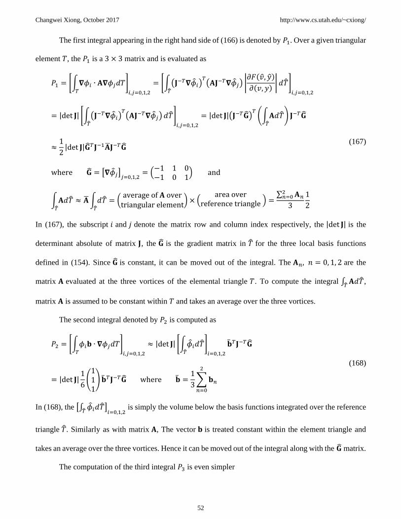
Changwei Xiong, October 2017 http://www.cs.utah.edu/~cxiong/
52
The first integral appearing in the right hand side of (166) is denoted by 𝑃1. Over a given triangular
element 𝑇, the 𝑃1 is a 3 × 3 matrix and is evaluated as
𝑃1 = [∫𝛁𝜙𝑖 ∙ 𝐀𝛁𝜙𝑗𝑑𝑇𝑇
]𝑖,𝑗=0,1,2
= [∫(𝐉−𝑇𝛁�̂�𝑖)𝑇(𝐀𝐉−𝑇𝛁�̂�𝑗) |
𝜕𝐹(�̂�, �̂�)
𝜕(𝑣, 𝑦)| 𝑑�̂�
�̂�
]𝑖,𝑗=0,1,2
= |det 𝐉| [∫(𝐉−𝑇𝛁�̂�𝑖)𝑇(𝐀𝐉−𝑇𝛁�̂�𝑗)
�̂�
𝑑�̂�]𝑖,𝑗=0,1,2
= |det 𝐉|(𝐉−𝑇�̂�)𝑇(∫𝐀𝑑�̂��̂�
) 𝐉−𝑇�̂�
≈1
2|det 𝐉|�̂�𝑇𝐉−1�̅�𝐉−𝑇�̂�
where �̂� = [𝛁�̂�𝑗]𝑗=0,1,2 = (−1 1 0−1 0 1
) and
∫𝐀𝑑�̂��̂�
≈ �̅�∫𝑑�̂��̂�
= (average of 𝐀 overtriangular element
) × (area over
reference triangle ) =∑ 𝐀𝑛2𝑛=0
3
1
2
(167)
In (167), the subscript 𝑖 and 𝑗 denote the matrix row and column index respectively, the |det 𝐉| is the
determinant absolute of matrix 𝐉, the �̂� is the gradient matrix in �̂� for the three local basis functions
defined in (154). Since �̂� is constant, it can be moved out of the integral. The 𝐀𝑛, 𝑛 = 0, 1, 2 are the
matrix 𝐀 evaluated at the three vortices of the elemental triangle 𝑇. To compute the integral ∫ 𝐀𝑑�̂��̂�
,
matrix 𝐀 is assumed to be constant within 𝑇 and takes an average over the three vortices.
The second integral denoted by 𝑃2 is computed as
𝑃2 = [∫𝜙𝑖𝐛 ∙ 𝛁𝜙𝑗𝑑𝑇𝑇
]𝑖,𝑗=0,1,2
≈ |det 𝐉| [∫�̂�𝑖𝑑�̂��̂�
]𝑖=0,1,2
�̅�𝑇𝐉−𝑇�̂�
= |det 𝐉|1
6(111) �̅�𝑇𝐉−𝑇�̂� where �̅� =
1
3∑𝐛𝑛
2
𝑛=0
(168)
In (168), the [∫ �̂�𝑖𝑑�̂��̂�]𝑖=0,1,2
is simply the volume below the basis functions integrated over the reference
triangle �̂�. Similarly as with matrix 𝐀, The vector 𝐛 is treated constant within the element triangle and
takes an average over the three vortices. Hence it can be moved out of the integral along with the �̂� matrix.
The computation of the third integral 𝑃3 is even simpler

Changwei Xiong, October 2017 http://www.cs.utah.edu/~cxiong/
53
𝑃3 = [∫𝜙𝑖𝜙𝑗𝑑𝑇𝑇
]𝑖,𝑗=0,1,2
= |det 𝐉| [∫�̂�𝑖�̂�𝑗𝑑�̂��̂�
]𝑖,𝑗=0,1,2
= |det 𝐉|1
24(2 1 11 2 11 1 2
) (169)
It is obvious that 𝑃1, 𝑃2 and 𝑃3 are all 3 × 3 matrix and just 𝑃2 appears asymmetric. Within each
element triangle, we have
[∫𝜙𝑖ℒ𝜙𝑗𝑑𝑇𝑇
]𝑖,𝑗=0,1,2
= 𝜎(𝑃1 + 𝑃2) + 𝑐𝑃3 and
[∫𝜙𝑖ℛ𝜙𝑗𝑑𝑇𝑇
]𝑖,𝑗=0,1,2
= (𝜎 − 1)(𝑃1 + 𝑃2) + (𝑐 − 𝑟)𝑃3
(170)
Aggregating integrals over all the triangular elements in the domain, the global stiffness matrix 𝒮 and
mass matrix ℳ can then be assembled.
3.2.3. Iterative Linear Solvers
3.2.3.1. Implementation of Sparse Matrix
As one can see, due to the use of localized basis functions, each node can interact with at most,
including itself, seven nodes. The stiffness and mass matrix can therefore be sparse. Since this is a 2-D
problem, as the resolution increases, the storage for the matrix increases quadratically. To avoid the
unnecessary memory storage for the zeros, a sparse matrix implementation is developed. The rows of a
sparse matrix are implemented as an array. Each entry of the array consists of a map, which maps the
column index to the matrix entry. Each map stores all the nonzero elements of a row vector of the sparse
matrix. Given a matrix index 𝑖 and 𝑗, it first finds the i-th row through the map array, and then locate the
j-th column entry through the i-th map. Using this implementation one can easily and efficiently access
the matrix members. This turns out to be very handy for constructing the sparse matrices.
Since the matrix is generally very large, for example, a 100 × 100 domain will generate (roughly)
a 10000 × 10000 matrix. In order to apply the iterative methods for the linear system, the matrix-vector
multiplication operation must be extremely efficient. To address this issue, the fully constructed sparse
matrix is then converted to a compressed row storage format, which consists of only three arrays: two

Changwei Xiong, October 2017 http://www.cs.utah.edu/~cxiong/
54
arrays store the matrix indices 𝑖 and 𝑗 respectively, and one array stores the corresponding matrix entries.
Although adding or removing the matrix entries is no longer as straightforward as before, the matrix
multiplications can be done very efficiently.
3.2.3.2. Iterative Methods for Asymmetric Sparse Matrix
The linear systems resulted from this problem are usually very large. Traditional direct method
and simple iterative methods are no longer appropriate for this type of applications. Furthermore, as one
can see that the 𝑃2 in (168) is asymmetric, and so is the global stiffness matrix 𝒮. In this case, the widely
used Conjugate Gradient method is no longer applicable. Instead, the Conjugate Gradient Squared (CGS)
and/or Generalized Minimal Residual (GMRES) method must be used to solve the linear systems. Since
the two methods have been widely documented, the details of the algorithm will not be described here.
The implementation of the two methods is based on Kelley’s book [28]. In general, CGS method performs
faster than GMRES method as it has much fewer floating point operations in each iteration, however in
some cases CGS method does not guarantee a convergence. In our application, the tolerance for
convergence is set to 1.0 × 10⁻⁸.
3.2.4. Interpolation of Numerical Solution
Numerical solution to the PDE is provided as a vector 𝑤 with values at each of the prescribed
nodes. To obtain a solution for an arbitrary position in the domain, interpolation must be performed. Since
the mesh can be either structured or unstructured, bilinear interpolation is not always appropriate. In this
case, the point coordinate is converted to a barycentric coordinate in an element triangle to perform the
linear interpolation. Firstly, it is desired to determine the triangle where the point locates. Given a point
coordinate (𝑣, 𝑦), the barycentric coordinates 𝜆0, 𝜆1, and 𝜆2 at this point can be computed based upon the
three triangle vortices ((𝑣0, 𝑦0), (𝑣1, 𝑦1), (𝑣2, 𝑦2))
(𝜆0𝜆1) = (
𝑣0 − 𝑣2 𝑣1 − 𝑣2𝑦0 − 𝑦2 𝑦1 − 𝑦2
)−1
(𝑣 − 𝑣2𝑦 − 𝑦2
) , 𝜆2 = 1 − 𝜆0 − 𝜆1 (171)
If 𝜆𝑖 ∈ [0,1] ∀ 𝑖 = 0,1,2, then the point is inside the triangle and the interpolated solution is
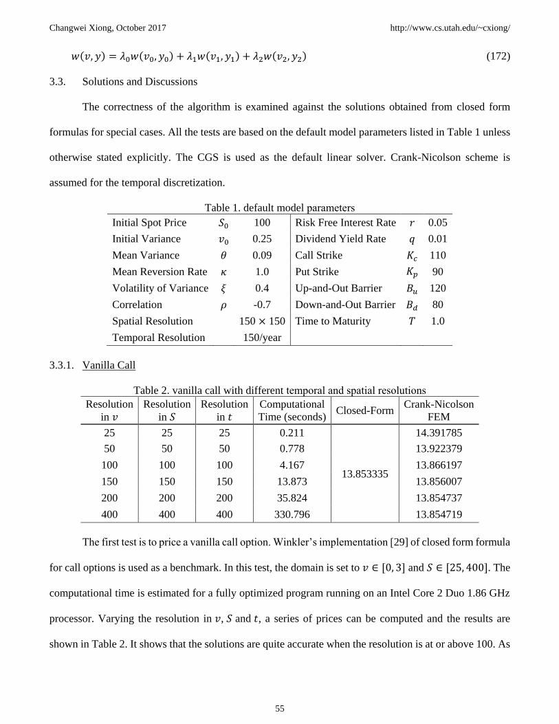
Changwei Xiong, October 2017 http://www.cs.utah.edu/~cxiong/
55
𝑤(𝑣, 𝑦) = 𝜆0𝑤(𝑣0, 𝑦0) + 𝜆1𝑤(𝑣1, 𝑦1) + 𝜆2𝑤(𝑣2, 𝑦2) (172)
3.3. Solutions and Discussions
The correctness of the algorithm is examined against the solutions obtained from closed form
formulas for special cases. All the tests are based on the default model parameters listed in Table 1 unless
otherwise stated explicitly. The CGS is used as the default linear solver. Crank-Nicolson scheme is
assumed for the temporal discretization.
Table 1. default model parameters
Initial Spot Price 𝑆0 100 Risk Free Interest Rate 𝑟 0.05
Initial Variance 𝑣0 0.25 Dividend Yield Rate 𝑞 0.01
Mean Variance 𝜃 0.09 Call Strike 𝐾𝑐 110
Mean Reversion Rate 𝜅 1.0 Put Strike 𝐾𝑝 90
Volatility of Variance 𝜉 0.4 Up-and-Out Barrier 𝐵𝑢 120
Correlation 𝜌 -0.7 Down-and-Out Barrier 𝐵𝑑 80
Spatial Resolution 150 × 150 Time to Maturity 𝑇 1.0
Temporal Resolution 150/year
3.3.1. Vanilla Call
Table 2. vanilla call with different temporal and spatial resolutions
Resolution
in 𝑣
Resolution
in 𝑆
Resolution
in 𝑡 Computational
Time (seconds) Closed-Form
Crank-Nicolson
FEM
25 25 25 0.211
13.853335
14.391785
50 50 50 0.778 13.922379
100 100 100 4.167 13.866197
150 150 150 13.873 13.856007
200 200 200 35.824 13.854737
400 400 400 330.796 13.854719
The first test is to price a vanilla call option. Winkler’s implementation [29] of closed form formula
for call options is used as a benchmark. In this test, the domain is set to 𝑣 ∈ [0, 3] and 𝑆 ∈ [25, 400]. The
computational time is estimated for a fully optimized program running on an Intel Core 2 Duo 1.86 GHz
processor. Varying the resolution in 𝑣, 𝑆 and 𝑡, a series of prices can be computed and the results are
shown in Table 2. It shows that the solutions are quite accurate when the resolution is at or above 100. As

Changwei Xiong, October 2017 http://www.cs.utah.edu/~cxiong/
56
one can see, the CGS solver performs very well. It takes only 5.5 minutes to solve a problem with
resolution as large as 400 × 400 × 400.
To examine the convergence property with respect to resolution in time, the spatial resolution is
fixed at 150 × 150, the temporal resolution varies from 5 to 200. The results are listed in Table 3. It shows
that the result is still acceptable even with a temporal resolution down to 5. The accuracy is improved
rapidly as the temporal resolution increases.
Table 3. vanilla call with different temporal resolutions
temporal resolution Computational
Time (seconds) Closed-Form
Crank-Nicolson
FEM
5 4.217
13.853335
13.761879
10 4.883 13.814776
20 5.879 13.835519
50 8.220 13.849429
100 11.414 13.854338
200 16.155 13.856847
The vanilla call prices are also evaluated at different strikes and shown in Table 4. The computed
prices are in excellent agreement with the closed form solutions. It should be noted that the computational
domain must be adjusted accordingly for the strike of 200 due to its large value. Since the call option with
a strike of 200 is far out of the money, it is expected that there is a relative large error in the computed
option price. This can be seen from the last row of the Table 4.
Table 4. vanilla call with different strikes
Strike 𝐾 Closed-Form Crank-Nicolson
FEM
105 15.935692 15.939498
110 13.853335 13.856007
115 11.975267 11.980188
130 7.4758044 7.4790939
150 3.6874922 3.6916604
200 0.42266949 0.43570695

Changwei Xiong, October 2017 http://www.cs.utah.edu/~cxiong/
57
Table 5. vanilla call with different maturities
Maturity Time
𝑇 Closed-Form
Crank-Nicolson
FEM
1/12 2.180542 2.1765933
1/4 5.7929266 5.7890237
1/2 9.3177983 9.3154635
1 13.853335 13.856007
2 19.56252 19.44822
5 29.918653 28.500867
10 N/A 36.782293
Resolutions increase from 150 to 300:
5 29.918653 28.938853
Figure 3. A typical solution surface for a vanilla call
Table 5 shows the computed option price with different maturity times. As compared with the
closed form solutions, the agreement is excellent except for those long term maturities (5 years and up).
Larger domain and higher resolutions can improve the accuracy. This has been shown for the case of 5

Changwei Xiong, October 2017 http://www.cs.utah.edu/~cxiong/
58
years maturity time. A typical solution surface for the vanilla call options is shown in Figure 3. Note that
the axis for sport process has been log transformed to 𝑦 = ln𝑆
𝐾.
3.3.2. Vanilla Put
The second test is to price a vanilla put option. In order to compare the results with closed form
solutions, the dividend rate 𝑞 = 0 is assumed. Rouah-Vainbergh’s Excel spreadsheet [30] is used as a
benchmark, which analytically solves for the put option price. In this test, the domain is also set as 𝑣 ∈
[0, 3] and 𝑆 ∈ [25, 400]. The put price is evaluated at different strikes. The results are shown in the Table
6. The computed prices are in excellent agreement with the closed form solutions, except for the strike of
20 due to the extreme out-of-the-money. It should be noted that the computational domain must be
adjusted accordingly for small strikes.
Table 6. vanilla put with different strikes
Strike 𝐾 Rouah-Vainbergh’s
Spreadsheet
Crank-Nicolson
FEM
95 N/A 11.816262
90 9.8286519 9.8259365
85 8.0667635 8.0587285
70 3.9702575 3.9744305
50 1.0635452 1.0610897
20 0.0118353 0.018820474
Table 7. vanilla put with different maturities
Maturity Time
𝑇
Rouah-Vainbergh’s
Spreadsheet
Crank-Nicolson
FEM
1/12 1.8136404 1.8153803
1/4 4.6993203 4.7001984
1/2 7.2118815 7.2117123
1 9.8286519 9.8259365
2 N/A 11.796426
Table 7 shows the computed put prices with different maturities. As compared with the benchmark
values, the computed prices are very close to the closed form solutions. A typical solution surface for the
vanilla put options is shown in Figure 4.

Changwei Xiong, October 2017 http://www.cs.utah.edu/~cxiong/
59
Figure 4. A typical solution surface for a vanilla put
3.3.3. Double Barrier Knock-out Call
Table 8. double barrier knock-out call with different barriers and strikes
Down Barrier Up Barrier Strike 𝐾 Faulhaber’s
Spreadsheet
Crank-Nicolson
FEM
20 200 110 5.99628132 5.986791
50 150 110 1.296335529 1.2971659
80 120 110 0.006384768 0.0066368712
20 200 100 8.812262221 8.8034578
50 150 100 2.655277021 2.6582231
80 120 100 0.051849246 0.053989178
20 200 90 12.51875619 12.510153
50 150 90 4.766805909 4.7734182
80 120 90 0.166447999 0.17333944
Resolutions increase from 150 to 300:
80 120 90 0.166447999 0.16993712

Changwei Xiong, October 2017 http://www.cs.utah.edu/~cxiong/
60
The third test is to price double barrier knock-out call options. To allow the existence of closed
form solutions, the correlation 𝜌 = 0 and the dividend rate, 𝑞 = 𝑟, the risk free interest rate are assumed.
Faulhaber’s Excel spreadsheet [31] is used as a benchmark, which analytically solve for the double barrier
option prices. In this test, the domain is assumed as 𝑣 ∈ [0, 3] and 𝑆 ∈ [𝐵𝑑 , 𝐵𝑢], The double barrier call
price is evaluated with different strikes and barriers. The results are shown in Table 8. The differences
between the computed prices and the closed form solutions are quite small, except for those close-to-zero
prices, in which the problems are ill-conditioned and are very difficult for the solver to compute a solution
accurately. As shown in the table, higher resolution can improve the accuracy.
Table 9 shows the computed double barrier knock-out call prices with different maturity times. To
avoid the close-to-zero prices, the down barrier 𝐵𝑑 = 50 and the up barrier 𝐵𝑢 = 150 are assumed. As
compared with the benchmark values, the numerical solutions are accurate, especially for the short term
options. A typical solution surface for the double barrier knock-out call options is shown in Figure 5. To
avoid the out-of-the-money, the barriers have been assume to be 𝐵𝑑 = 50 and 𝐵𝑢 = 150.
Table 9. vanilla put with different maturities
Maturity Time
𝑇
Rouah-Vainbergh
Spreadsheet
Crank-Nicolson
FEM
1/12 2.073151427 2.056223
1/4 2.748504846 2.7439708
1/2 2.048575635 2.049062
1 1.296335529 1.2971659
2 0.744555858 0.77808438

Changwei Xiong, October 2017 http://www.cs.utah.edu/~cxiong/
61
Figure 5. A typical solution surface for a double barrier knock-out call
3.3.4. Double Barrier Knock-out Put
Table 10. double barrier knock-out put with different barriers and strikes
Down Barrier Up Barrier Strike 𝐾 Faulhaber’s
Spreadsheet
Crank-Nicolson
FEM
20 200 110 21.87927024 21.872058
50 150 110 12.46280153 12.452305
80 120 110 0.235744502 0.24543624
20 200 100 15.93365322 15.927314
50 150 100 8.307725123 8.2976528
80 120 100 0.090320836 0.094025866
20 200 90 10.87854926 10.872598
50 150 90 4.905236115 4.8971387
80 120 90 0.014031445 0.014613467
The fourth test is to price a double barrier knock-out put option. In this case, the correlation 𝜌 = 0
and the dividend rate, 𝑞 = 𝑟, the risk free interest rate are assumed. Faulhaber’s excel spreadsheet is once
again used as a benchmark. In this test, the domain is 𝑣 ∈ [0, 3] and 𝑆 ∈ [𝐵𝑑 , 𝐵𝑢]. The double barrier put

Changwei Xiong, October 2017 http://www.cs.utah.edu/~cxiong/
62
price is evaluated with different strikes and barriers. The results are shown in Table 10 and Table 11. The
computed prices are in good agreement with the closed form solutions. As usual, higher resolution leads
to a better accuracy.
Table 11. double barrier knock-out put with different strikes
Down
Barrier
Up
Barrier
Strike
𝐾
Faulhaber’s
Spreadsheet
Crank-Nicolson FEM
Resolutions: 150 Resolutions: 300
80 120 110 0.235744502 0.24543624 0.24058918
80 120 100 0.090320836 0.094025866 0.092165229
80 120 90 0.014031445 0.014613467 0.014317593
Table 12 shows the computed double barrier knock-out put prices with different maturity times.
To avoid the close-to-zero prices, the down barrier 𝐵𝑑 = 50 and up barrier 𝐵𝑢 = 150 are assumed. A
typical solution surface for the double barrier double barrier knock-out put options is shown in Figure 6.
As compared with the benchmark values, the numerical solutions are accurate, especially for the short
term options.
Table 12. double barrier knock-out put with different maturities
Maturity Time
𝑇
Rouah-Vainbergh
Spreadsheet
Crank-Nicolson
FEM
1/12 1.790372434 1.7880031
1/4 4.564088509 4.5554437
1/2 5.606674031 5.5991206
1 4.905236115 4.8971387
2 3.368687428 3.3595535

Changwei Xiong, October 2017 http://www.cs.utah.edu/~cxiong/
63
Figure 6. A typical solution surface for a double barrier knock-out put
3.3.5. Numerical Solutions of Double Barrier Knock-out Options
The Crank-Nicolson finite element solver is used to price the double barrier options for our
problem. Specifically, the double barrier options are assumed to follow Heston stochastic volatility model
and take the values for the parameters as listed in Table 1. The computation is performed on a domain
defined as 𝑣 ∈ [0, 3] and 𝑆 ∈ [𝐵𝑑 , 𝐵𝑢]. The spatial and temporal resolutions are set to various levels to
gain an overview about the accuracy and convergence trend. The solutions are shown in Table 13. Since
these two option prices are very close to zero, the results computed at lower resolutions may have large
errors. As the resolution improves, we do see the convergence of the solution. Another observation is that
at the same resolution the computational time for double barrier options is much longer than that of plain
vanilla options. This is partially because that double barrier options usually have more dynamic features
than plain vanillas and therefore they are more computationally challenging.

Changwei Xiong, October 2017 http://www.cs.utah.edu/~cxiong/
64
Table 13. Double Barrier Knock-out Options
Type Resolution
(spatial and temporal)
Computational Time
(seconds) Computed Price
Call
100 30.6 0.019140956
150 125.9 0.014483851
200 367.1 0.012706429
300 1328.3 0.011207521
400 3942.1 0.010623075
500 9174.5 0.010275859
Put
100 28.9 0.0047008941
150 138.2 0.0045130817
200 325.7 0.0044583508
300 1399.3 0.0044205309
400 3698.4 0.0044209021
500 9461.7 0.0044168854
3.4. Conclusions
It has been illustrated how to price a double barrier knock-out option (the knock-in type barrier
options can be priced in a similar manner, except that the vanilla option prices are used for Dirichlet
boundaries) in a stochastic volatility model using finite element method. The numerical solutions of the
testing cases are in excellent agreement with the closed form values. This strongly suggests the accuracy
and efficiency advantages of this method, as compared with finite difference method and Monte Carlo
simulations. With appropriate boundary condition definitions, this method can be easily extended to price
more complicated exotic options. It can also be further improved by applying adaptive mesh refinement
and/or higher order basis functions.

Changwei Xiong, October 2017 http://www.cs.utah.edu/~cxiong/
65
REFERENCES
1. Clark, I., Foreign Exchange Option Pricing - A Practitioner’s Guide, Wiley-Finance, 2011, pp.82
2. Shreve, S., Stochastic Calculus for Finance II Continuous-Time Models, Springer Finance, 2004
3. Janek, A.; Kluge, T.; Weron, R. and Wystup, U., “FX smile in the Heston model,” Chapter 4 in
Statistical Tools for Finance and Insurance (2nd Ed), Cizek et al. (eds.), Springer-Verlag, 2011.
4. Clark, I., Foreign Exchange Option Pricing - A Practitioner’s Guide, Wiley-Finance, 2011, pp.98
5. Dragulescu, A. and Yakovenko, V., Probability distribution of returns in the Heston model with
stochastic volatility, Quantitative Finance 2: 443–453. 2002
6. del Bano Rollin, S.; Ferreiro-Castilla, A.; Utzet, F., On the density of log–spot in the Heston volatility
model, Stoch. Process. Appl. 120, 2037–2063 (2010)
7. Online resource: http://www.ems.bbk.ac.uk/for_students/msc_finEng/math_methods/lecture7.pdf
8. Wikipage: http://en.wikipedia.org/wiki/Characteristic_function_(probability_theory)
9. Duffie, D., Dynamic Asset Pricing Theory, 3rd Ed, Princeton University Press, 2001, pp.180
10. Wu, L., Chapter 3 Modeling Financial Security Returns Using Lévy Processes, pp.150, in
“Handbooks in Operations Research and Management Science, Vol 15, Financial Engineering”
edited by Birge, J. and Linetsky, V., Elsevier Science, 2008
11. Online resource: http://www.math.nus.edu.sg/~matsr/ProbI/Lecture6.pdf
12. Schmelzle, M., Option Pricing Formulae using Fourier Transform: Theory and Application, 2010,
pp.10, Online resource: http://pfadintegral.com/docs/Schmelzle2010%20Fourier%20Pricing.pdf
13. Elices, A., Models with Time-Dependent Parameters using Transform Methods: Application to
Heston’s Model, “Appendix A: Deriving the Characteristic Function”, arXiv.org, Oct. 20, 2008
Online resource: http://arxiv.org/ftp/arxiv/papers/0708/0708.2020.pdf
14. Wu, L., From Characteristic Functions and Fourier Transforms to PDF’s-CDF’s, online resource:
http://faculty.baruch.cuny.edu/lwu/890/ADP_Transform.pdf
15. Wu, L., Chapter 3 Modeling Financial Security Returns Using Lévy Processes, pp.150, in
“Handbooks in Operations Research and Management Science, Vol 15, Financial Engineering”
edited by Birge, J. and Linetsky, V., Elsevier Science, 2008
16. Wu, L., Chapter 3 Modeling Financial Security Returns Using Lévy Processes, pp.152, in
“Handbooks in Operations Research and Management Science, Vol 15, Financial Engineering”
edited by Birge, J. and Linetsky, V., Elsevier Science, 2008
17. Schmelzle, M., Option Pricing Formulae using Fourier Transform: Theory and Application, 2010,
pp.24, Online resource: http://pfadintegral.com/docs/Schmelzle2010%20Fourier%20Pricing.pdf
18. Schmelzle, M., Option Pricing Formulae using Fourier Transform: Theory and Application, 2010,
pp.17
Online resource: http://pfadintegral.com/docs/Schmelzle2010%20Fourier%20Pricing.pdf
19. Albrecher, H.; Mayer, P.; Schoutens, W. and Tistaert, J., The little Heston trap, Wilmott Magazine,

Changwei Xiong, October 2017 http://www.cs.utah.edu/~cxiong/
66
January 2006: 83–92. 231–262.
20. Elices, A., Models with Time-Dependent Parameters using Transform Methods: Application to
Heston’s Model, arXiv.org, Oct. 20, 2008
Online resource: http://arxiv.org/ftp/arxiv/papers/0708/0708.2020.pdf
21. F. Black and M. Scholes, The pricing of options and corporate liabilities, Journal of Political
Economy, pp. 637-654, 1973
22. Heston, S., A closed-form solutions for options with stochastic volatility, Review of Financial Studies,
6, 327–343, 1993
23. Topper, J. Financial Engineering with Finite Elements, Wiley Finance Series, 2005
24. Winkler, G.; Apel, T.; Wystup, U., Valuation of options in Heston's stochastic volatility model using
finite element methods, in J. Hakala, U. Wystup (eds.) Foreign Exchange Risk, Risk Books, London,
2002
25. Achdou, Y.; Tchou, N., Variational analysis for the Black-Scholes equation with stochastic volatility,
ESAIM: Mat. Mod. and Num. Analysis, 36/3, 373-395, 2002
26. Miglio, E.; Sgarra, C., A Finite Element Framework for Option Pricing with the Bates Model,
Computing and Visualization in Science, in publish, 2009
27. Gockenbach, M., Understanding And Implementing the Finite Element Method, SIAM, 2006
28. Kelley, T., Iterative Methods for Linear and Nonlinear Equations, SIAM, 2004
29. Online resource: http://www.guwi17.de/heston/index.html
30. Rouah, F.; Vainberg, G., Option Pricing Models and Volatility Using Excel-VBA, Wiley Finance,
2007
31. Faulhaber, O., Analytic methods for pricing double barrier options in the presence of stochastic
volatility, Master's thesis, Mathematics Department, University of Kaiserslautern, Germany, 2002