value investing on the nordic stock market - lund...

Department of Economics

NEKH01 – Bachelor Thesis

Fall 2016

Value Investing on the Nordic Stock Market

Does the Magic Formula constitute a viable strategy for outperforming the market?

Authors: Supervisor: Emil Håkansson Dag Rydorff Pontus Kvarnmark

1

Abstract In this thesis we investigate if following the magic formula can yield superior investment

returns in relation to the risk taken. The magic formula is a term coined by Joel

Greenblatt, describing a systematic approach to successful stock investing. The strategy

identifies high value companies based on return on capital that are selling at a discount

to their intrinsic value based on the company’s earnings yield. In order to examine the

possible relation between the magic formula and superior investment returns, we back-

test the formula on the Nordic stock market between 2007 and 2016. We compare the

returns of the portfolio with the benchmark OMX Nordic 40. In order to determine if the

portfolio has yielded high returns in relation to each unit of risk, we apply the Capital

Asset Pricing Model as well as the Fama-French three-factor model. Using the CAPM for

the period 2007 to 2016 we arrive at a monthly excess return of 1.27% and an annual

excess return of 17.8%. Applying the three-factor model, we yield a monthly and annual

excess return of 1.29% and 14.01% respectively. Excess returns are often attributed to

having taken on excess risk or merely as the result of chance. The Sharpe ratio for the

period 2007 to 2016 was 0.22 for the magic formula portfolio compared to 0.027 for the

OMX Nordic 40. Testing if the Sharpe ratio of the magic formula is different from the

Sharpe ratio of the market, it is evident that the results are statistically significant. The

years following the financial crisis of 2008 are included in the test period. It is notable

that although the magic formula portfolio is significantly less diversified than the OMX

Nordic 40, it performed better during the setback of 2008 and 2009, and returned to

pre-crisis levels more rapidly than the market portfolio.

Key words: Value Investing, Sharpe Ratio, Nordic Stock Market, Magic Formula, CAPM, Fama-French three-factor model

2

Contents 1. Introduction ........................................................................................................................... 4

1.1 Purpose ........................................................................................................................................... 5

1.2 Results ............................................................................................................................................. 5

1.3 Outline ............................................................................................................................................. 6

2. Theory ...................................................................................................................................... 7

2.1 The Efficient Market Hypothesis .......................................................................................... 7

2.2 Anomalies ...................................................................................................................................... 9

2.2.1 The January Effect .............................................................................................................. 9

2.2.2 Price Earnings Effect ......................................................................................................... 9

2.3 Value Investing ......................................................................................................................... 10

2.4 Theoretical Models .................................................................................................................. 12

2.4.1 The Capital Asset Pricing Model ................................................................................ 12

2.4.2 Three-Factor Model ........................................................................................................ 13

2.4.3 Sharpe Ratio ...................................................................................................................... 14

2.5 Definitions .................................................................................................................................. 16

2.5.1 EBIT ...................................................................................................................................... 16

2.5.2 Return on Capital ............................................................................................................. 17

2.5.3 Enterprise Value .............................................................................................................. 17

2.5.4 Earnings Yield ................................................................................................................... 17

2.5.5 Systematic risk ................................................................................................................. 18

3. Magic Formula Theory .................................................................................................... 19

3.1 Introduction ............................................................................................................................... 19

3.2 The Magic Formula .................................................................................................................. 19

3.3 Ranking ........................................................................................................................................ 20

3.4 Magic Formula Risk ................................................................................................................. 21

3.5 Prior Research (Magic Formula) ........................................................................................ 22

4. Data & Method .................................................................................................................... 24

4.1 Data ............................................................................................................................................... 24

4.2 Method ......................................................................................................................................... 25

4.3 Problems ..................................................................................................................................... 29

5. Results & Analysis ............................................................................................................. 31

5.1 Absolute Returns ..................................................................................................................... 31

5.2 Volatility ...................................................................................................................................... 32

3

5.3 Capital Asset Pricing Model ................................................................................................. 36

5.4 Three-Factor Model ................................................................................................................ 36

5.5 Sharpe Ratio ............................................................................................................................... 37

6. Conclusions ......................................................................................................................... 39

7. Further Research .............................................................................................................. 41

8. References ........................................................................................................................... 42

9. Appendix .............................................................................................................................. 44

9.1 Databases .................................................................................................................................... 44

9.2 Portfolios ..................................................................................................................................... 44

9.3 Removed Companies .............................................................................................................. 50

9.4 Performance .............................................................................................................................. 53

9.5 Datastream formulas .............................................................................................................. 55

4

1. Introduction The principal theory among academics and institutional investors in recent years has

become the theory of efficient markets. Originally explained by Fama (1970), the

hypothesis states that the pursuit of excess returns on the financial markets is folly, as

asset prices always reflect all available information. Fama (1970) argues that excess

returns over a given time period are merely the result of either chance or of taking on

excess risk.

This understanding of financial markets has gained criticism from a group within the

investing community called value investors. Perhaps the most widely recognized

advocate of value investing is Warren Buffett, who on several occasions has questioned

the implications of the efficient market hypothesis (Buffett, 1989). Proponents of a

value-approach to investing argue, as advocated in Buffett’s 1984 article entitled The

Super Investors of Graham-and-Doddsville, that the probability of several investors, all

following the same investment philosophy, consistently outperforming the market,

could not be explained by mere chance (Buffett, 1984).

A disciple of the value investing school is hedge fund manager Joel Greenblatt, who

through a systematic approach to stock-picking which he calls magic formula investing,

identifies high value companies based on return on capital that are selling at a discount

to their intrinsic value based on the company’s earnings yield. Greenblatt has

successfully implemented this strategy on the American stock exchange over a

significant period of time (Greenblatt, 2006).

We attempt to measure whether having applied Greenblatt’s magic formula on the

Nordic stock exchange from the period 2007 to 2016 would have yielded satisfactory

returns in relation to the risk that would have been taken on and if the magic formula is

likely to produce similar results in the future.

5

1.1 Purpose

The purpose of this thesis is to investigate the risk-adjusted performance of a portfolio,

constructed using Joel Greenblatt’s magic formula framework, on the Nordic stock

market between the years 2007 and 2016 and to determine if the formula constitutes a

viable strategy for outperforming the market in the future.

1.2 Results

The results we obtain from back-testing Greenblatt’s strategy on the Nordic stock

market are quite intriguing. Having applied the magic formula on the Nordic stock

market from 2007 to 2016 would have yielded a monthly and annual excess return of

1.27% and 17.8% respectively. We conclude that the returns are not merely the result

of taking on excess risk. In 83 out of the total 108 months, the volatility as measured by

the standard deviation of the portfolio was lower than the market portfolio,

represented by the OMX Nordic 40. The average monthly volatility was also lower for

the magic formula portfolio: 1.1% for the magic formula portfolio compared to 1.2% for

the OMX Nordic 40. The Sharpe-ratio, expressing the total yield gained per unit of risk

taken, is significantly higher for the magic formula: 0.22 as compared to the OMX Nordic

40 which had a Sharpe-ratio of 0.03. We apply the hypothesis test from Jobson and

Korkie (1981) to determine if the difference between the Sharpe ratio of the magic

formula portfolio and the OMX Nordic 40 is statistically significant, we find that that the

Sharpe ratio of the magic formula is significantly higher than that of the OMX Nordic 40,

and not merely the result of chance. In order to determine if the excess return can be

explained by having been exposed to a high degree systematic risk, we apply the Capital

Asset Pricing Model. Furthermore, we apply the Fama-French three-factor model, which

attempts to explain the excess return of the portfolio by adding two more factors to the

CAPM, a value factor and a size factor. As for the CAPM and Fama-French three-factor

model, we receive positive alpha-values and beta values between 0 and 1. This indicates

that the returns are not the result of the magic formula strategy taking on excess risk.

6

As the financial crisis of 2008 is included in the test period, it is clear that, although the

magic formula portfolio is less diversified than the market portfolio, it performed better

during the years of the crisis and recovered much more rapidly than the market

portfolio did. Thus, the results of the investigation indicate that applying the magic

formula on the Nordic stock market will yield returns that are quite satisfactory.

1.3 Outline In the subsequent section we provide the theoretical framework that the investigation is

based on. We introduce the hypothesis of efficient markets and the implications it has

on active portfolio management and on the magic formula in particular. Further on, we

also discuss previous studies of efficient markets and anomalies that contradict the idea

of a strongly efficient market. In the theory section we also clarify the models that we

apply to determine the risk-adjusted returns such as The Capital Asset Pricing Model,

Fama-French three-factor model and the Sharpe Ratio. Following this we discuss the

framework behind Joel Greenblatt’s magic formula. How each company is ranked, how

the portfolios are constructed and how portfolio risk is calculated is included in this

section. The penultimate chapter, Data & Method, is concerned with how we interpret

and apply the magic formula to the Nordic Market. In this chapter we also explain the

compromises that we are forced to make, mainly due to a lack of data. In the last

section we analyze and discuss the results of the investigation and provide

recommendations for further research.

7

2. Theory

2.1 The Efficient Market Hypothesis

Fama (1970) proposes the idea of efficient markets. The hypothesis implies that

achieving superior returns over a long period is merely the result of luck or a result of

the investor taking on excess risk. As markets always reflect all available information,

investors cannot exploit information that the wider market does not have access to, as

no such information exists. The hypothesis suggests that attempting to manage a

portfolio actively is folly, arguing that the only way to achieve higher returns is to take

on excess risk.

The efficient market hypothesis differentiates between different levels of efficiency. The

least efficient level is weak market efficiency. Weak efficiency suggests that previous

movements in the price of a stock do not affect its future movements (Fama, 1970). This

implies that any strategy advocating the use of technical analysis to predict the future

movements of a stock cannot be used to gain superior returns. Weak market efficiency

also suggests that figures in a company’s balance sheet, income statement or other

fundamentals need not necessarily be reflected in the price of stock. Hence,

fundamental analysis can be used to find undervalued and overvalued stocks and thus

achieve superior returns.

Semi-strong market efficiency is defined as the market reflecting all publicly available

information. Hence, balance sheet figures, cash flow statements and the like cannot be

used to find undervalued or overvalued companies, as these figures are already

incorporated in the stock price (Fama, 1970). Semi-strong efficiency suggests that the

only information that can be exploited in order to achieve superior returns is

information that is not readily available to the general public. Insider information, that

is, information only available to a certain few within the company, is not reflected in the

stock price and could potentially be used to purchase undervalued companies.

8

The highest form of efficiency is strong market efficiency. The idea of strong market

efficiency suggests that all information is reflected in the price of a stock, both public

and private. Hence, neither public nor insider information could be exploited to gain

excess returns (Fama, 1970). The implications of strong market efficiency are that any

form of active portfolio management cannot be carried out successfully over a longer

period of time. Thus, investors should revert back to a passive form of investing such as

purchasing an index fund.

The efficient market hypothesis has implications on the magic formula. Weak market

efficiency suggests that the magic formula can possibly be used in order to purchase

companies with high profitability measures at a bargain price. However, the idea of

semi-strong and strong efficiency is contradictory to the idea of applying the magic

formula successfully. As semi-strong and strong efficiency imply that all publicly

available information, including such figures as return on capital, earnings before

interest and taxes, and enterprise value are already reflected in the stock price, any

attempt at purchasing a company at a bargain price will not yield satisfactory results.

Strong and semi-strong efficiency imply that having achieved superior returns over a

long period by using Joel Greenblatt’s formula is either the result of luck or of the

formula taking on excess risk.

9

2.2 Anomalies

2.2.1 The January Effect Among market anomalies, one of the most widely studied is the January effect. First

observed and described by Wachtel (1942) in Certain Observations on Seasonal

Movements in Stock Prices, the paper coined the term January effect, describing the

historically abnormal returns and “bullish tendencies” (Wachtel, 1942, p.185) of stocks

during the first month of the year.

Wachtel (1942) examines the returns of stocks in December to January on the Dow

Jones Industrial Average from 1927 to 1942 and finds that the index depreciates in only

four of the fifteen years. Another study indicating the existence of a January Effect,

Rozeff and Kinney (1976) find that the return on the New York Stock Exchange in

January from 1904 to 1974 was roughly eight times as high as the average monthly

return.

A plausible explanation of the January effect is the willingness to avoid paying excessive

amounts in taxes. A stock that has yielded negative returns over a given time period

could be sold at the end of the year in order to cancel out capital losses and capital

gains, thus minimizing capital gains tax. This large sell-off in the later months of the year

has the effect of driving down the prices of stocks. The recovery of stock prices in the

early months of the year, following the sell-off in December, offer an explanation to the

abnormally high returns historically observed in January.

2.2.2 Price Earnings Effect The P/E effect refers to the historical outperformance of stocks with low price-earnings

ratios compared to stocks with higher valuations. The price-earnings ratio is a measure

of how much a stock is trading for in relation to the earnings of the underlying company.

Companies that exhibit low growth potential are usually awarded a low P/E-ratio, while

10

companies with high P/E-ratios and high valuations, trade at a premium due to potential

growth in future earnings.

Basu (1977) studies the P/E-effect on the NYSE from 1956 to 1971. Companies are

ranked according to P/E-ratio and grouped into five portfolios. The paper finds that the

lowest P/E portfolio has an average annualized return of 16.3%, the highest P/E

portfolio exhibits an average annual return of 9.34%, and the returns of the three

middle portfolios decrease more or less monotonically as P/E ratios increase (Basu,

1977). Furthermore, Basu (1977) finds that the low P/E portfolios do not exhibit higher

systematic risk than the high P/E portfolios.

A possible explanation to this anomaly is investor psychology. If investors overestimate

future potential growth, too high a premium is paid for the stock. Inversely,

underestimating companies with low growth projections can potentially cause the stock

of a company to sell at a discount. On aggregate, earnings tend to revert back to the

mean. This inevitably causes a portfolio comprised of high P/E companies to

underperform a portfolio made up of the stocks of low P/E companies.

2.3 Value Investing

Value investing refers to the act of identifying and purchasing companies that are selling

at a bargain to their intrinsic value. Any sensible act of active investing is concerned with

purchasing companies that the investor considers undervalued. Hence, all active

investing can be described as value investing. However, traditionally value investing has

been defined as identifying undervalued companies based on some fundamental

measure such as a low price-earnings ratio, high earnings yield or the company selling

bellow net current asset value. Historically investing has been grouped into two distinct

categories, growth investing and value investing, a rather naive distinction, as growth

certainly is a component of a company’s value. However, for the sake of simplicity,

11

purchasing a company that upon analyzing the fundamentals of the business appears to

be undervalued is the essence of value investing.

Benjamin Graham of Columbia University is often ascribed as the father of value

investing (Graham, 1934). In his seminal work, Security Analysis, Benjamin Graham, in

collaboration with Professor David Dodd, provides the foundation for what is today

called value investing (Graham, 1934). Graham argues that the value of a company and

the price of the company’s stock are two different things. “Price is what you pay; value

is what you get” summarizes Grahams teachings (Buffett, 2009). Graham claims that the

discrepancies between price and value are often attributed to “exaggeration,

oversimplification or neglect” (Graham, 2009, p.669). Graham (1934) argues that

identifying and investing in companies selling below their intrinsic value could achieve

superior returns. This idea is not compatible with the efficient market hypothesis, which

argues that the market always reflects all available information and that market

participants act rationally.

Joel Greenblatt’s magic formula is rooted in the teachings of Benjamin Graham. The

magic formula attempts to identify companies that are selling at a bargain price in

relation to future earnings potential. While Graham looks to the stability of earnings,

dividend history and earnings growth as an indicator of future earnings, Greenblatt

focuses on return on invested capital as an indicator of a company’s future earnings

potential (Greenblatt, 2006). Graham relies heavily on company balance sheets in order

to determine the value of a company, with stocks selling below tangible book value or

below net current asset value indicating a low valuation (Graham, 2009). Greenblatt

substitutes these measures with earnings yield. Although the two investors use different

measures to identify possible investments, the reasoning remains the same; identify

companies with solid track records that display signs of future earnings potential, and

purchase these companies at a bargain to their intrinsic value.

12

2.4 Theoretical Models

2.4.1 The Capital Asset Pricing Model The capital asset pricing model is an economic model used for pricing an individual

security or portfolio. Using the model on a specific asset one can calculate the specific

asset’s expected return. The CAPM assumes that there is only one factor of risk, being

the market risk factor or systematic risk, usually depicted as Beta, 𝛽. The model explains

that the higher the beta of an asset, the higher the average return of the asset

(Cochrane 1999). The Beta itself is an estimation of how much the asset tends to move

with the market. A beta value of one implies that the asset is perfectly correlated with

the market, a beta value of negative one indicates that the asset is negatively correlated

with the market, and a beta of zero means that the asset is perfectly uncorrelated with

the market. The equation is as follows:

𝐸(𝑅𝑖) = 𝑅𝑓 + 𝛽𝑖(𝐸(𝑅𝑚) − 𝑅𝑓) (1)

Where:

𝐸(𝑅𝑖) = Expected return of asset i

Rf = Risk free rate of interest

𝛽𝑖 = Beta of asset i

𝐸(𝑅𝑚) = Expected return of the market

The model can also be used to determine if a portfolio’s returns exceed the expected

return, justified by the specific beta value. For this purpose we rearrange the equation

and add the symbol alpha, 𝛼, which is the sum of the actual return of the asset and the

expected return calculated with the CAPM (Womack, 2003). A positive alpha suggests

that the asset yields higher returns than the CAPM predicts. The result is presented

below:

𝐸(𝑅𝑖) − 𝑅𝑓 = 𝛼 + 𝛽𝑖(𝐸(𝑅𝑚) − 𝑅𝑓) (2)

13

2.4.2 Three-Factor Model The Fama-French three-factor model (Fama & French, 1993) is an expansion of the

Capital Asset Pricing Model. Resting on the foundation of the CAPM, the three-factor

model takes two more risk factors into account. These factors are the so-called size

factor and the value factor. These factors are often abbreviated as SMB and HML. SMB

or Small (market cap) Minus Big is the historical excess return that investors have

yielded when investing in small cap stocks compared to big cap companies. HML or High

Minus Low is the historical excess return that investors have yielded when investing in

value companies compared to growth companies. The HML value is calculated by

comparing the average returns of two portfolios comprised of growth stocks and two

portfolios comprised of value stocks. Similarly, the SMB value is the difference in

average returns between three small market cap portfolios and three big cap portfolios.

With these two variables added to the CAPM we find that the degree at which the

model explains the return of an asset is increased (Fama & French, 1993). Adding these

variables to the CAPM we end up with Equation 3. The 𝛽 remains the market risk

coefficient, and the 𝑠𝑖 and ℎ𝑖 measure the assets exposure to size and value factors.

𝐸(𝑅𝑖) = 𝑅𝑓 + 𝛽𝑖(𝐸(𝑅𝑚) − 𝑅𝑓) + 𝑠𝑖𝑆𝑀𝐵 + ℎ𝑖𝐻𝑀𝐿 (3)

Furthermore, the model can be rearranged in such a way as to so be used to evaluate

the performance of a portfolio, i.e. to determine if the investor yielded abnormal

returns due to skill or luck. Running a regression and evaluating the portfolio, one needs

to find the values for the SMB and HML factors, readily available from Kenneth French’s

homepage.1 To determine if their returns have been in excess, the alpha, 𝛼, is added to

the model. Please see Equation 4. If 𝛼 is positive after the regression has been carried

out and the results are deemed to be statistically significant, the portfolio’s returns are

greater than the model predicts, i.e. the portfolio has generated excess returns that are

1 http://mba.tuck.dartmouth.edu/pages/faculty/ken.french/data_library.html

14

not explained by higher exposure to the three factors, but are in fact due to a superior

investment strategy.

𝐸(𝑅𝑖) − 𝑅𝑓 = 𝛼 + 𝛽𝑖(𝐸(𝑅𝑚) − 𝑅𝑓) + 𝑠𝑖𝑆𝑀𝐵 + ℎ𝑖 𝐻𝑀𝐿 (4)

2.4.3 Sharpe Ratio The Sharpe ratio or risk-to-volatility measure is a measure of how much a financial asset

yields per unit of risk. The risk-averse investor in the United States has the opportunity

to purchase T-bills issued by the Federal Reserve of the United States, these financial

assets are deemed to be entirely risk-free. The Swedish equivalent is the

statsskuldsväxel (SSVX). If the investor requires a higher return than that which the risk-

free asset guarantees, excess risk has to be taken on. The Sharpe ratio, as proposed by

(Sharpe, 1994), measures how much the investor has yielded in relation to the risk taken

on. As the Sharpe ratio only requires three figures, the return, the risk-free rate and the

volatility or standard deviation, the ratio of different securities is readily comparable. As

proposed by Sharpe (1994), the Sharpe ratio is defined as:

𝑠𝑟𝑖 = 𝐸 (𝑅𝑖)−𝑅𝑓

𝜎𝑖 (5)

In order to determine if the difference between the Sharpe ratio of the magic formula

portfolio and the OMX Nordic 40 is statistically significant, we use the test statistics

derived by Jobson and Korkie (1981). Below, we present an outline of the methodology.

𝑑 = 𝐸[𝑅𝑖] − 𝑅𝑓 , Where d is the expected differential return (6)

𝑠𝑟𝑖 = 𝑑

𝜎𝑑 , The expected differential return per unit of risk (ex ante) (7)

Estimating the Sharpe ratio

𝑠�̂�𝑖 = 𝑚𝑖

𝑠𝑖 , The expected differential return per unit of risk (ex post) (8)

15

Where:

𝑚𝑖 =1

𝑇∑ 𝑑𝑖𝑡

𝑇𝑡=1 (9)

𝑠𝑖 = √1

𝑇∑ (𝑑𝑖𝑡 − 𝑚𝑖)2𝑇

𝑡=1 (10)

The differential return between the portfolio and market at time t: 𝑑𝑖𝑡 = (𝑅𝑖𝑡 − 𝑅𝑓𝑡) (11)

Significance Test Assume that the returns are independently and identically distributed (IID), and use the

following significance test:

𝐻0: 𝑠𝑟𝑖𝑗 ≡ 𝑠𝑟𝑖 − 𝑠𝑟𝑗 = 0 , The difference between the Sharpe ratio of the magic formula

and of the market is zero.

𝐻1: 𝑠𝑟𝑖𝑗 ≡ 𝑠𝑟𝑖 − 𝑠𝑟𝑗 ≠ 0 , The difference between the Sharpe ratio of the magic formula

and of the market is not zero.

Apply the transformed difference to calculate a value for 𝑠�̂�𝑖𝑗 :

𝑠�̂�𝑖𝑗 ≡ 𝑠�̂�𝑖 − 𝑠�̂�𝑗 = 𝑠𝑗𝑚𝑖 − 𝑠𝑖𝑚𝑗 (12)

The variance of the quotient between the Sharpe ratio of the magic formula and of the

market:

𝜃 =1

𝑇[2𝑠𝑖

2𝑠𝑗2 − 2𝑠𝑖𝑠𝑗𝑠𝑖𝑗 +

1

2𝑚𝑖

2𝑠𝑗2 +

1

2𝑚𝑗

2𝑠𝑖2 −

𝑚𝑖𝑚𝑗

2𝑠𝑖𝑠𝑗[𝑠𝑖𝑗

2 + 𝑠𝑖2𝑠𝑗

2]] (13)

The test statistics used to test the null hypothesis is:

𝑧(𝑠𝑟𝑖𝑗) = 𝑠�̂�𝑖𝑗

√𝜃~𝑁(0,1) (14)

16

A two-sided t-test is carried out using the following formula in Excel, with a significance

level of 5 percent:

P-value = 2 ∗ (1 − 𝑛𝑜𝑟𝑚. 𝑠. 𝑑𝑖𝑠𝑡 (𝑎𝑏𝑠 (𝑧(𝑠𝑟𝑖𝑗))) (15)

If the calculated p-value is less than 0.05, the null hypothesis is rejected and it is

concluded that the difference between the Sharpe ratio of the magic formula and the

market portfolio is statistically significant.

2.5 Definitions A few basic accounting terms are useful to understand in order to fully grasp the

reasoning behind the magic formula strategy. Greenblatt uses return on capital as a

way to quantify the profitability of a company and to gain a readily comparable measure

of how efficiently a company is creating shareholder value (Greenblatt, 2006). The

second ratio that the formula is concerned with is the earnings yield. The earnings yield

simply states the price an investor has to pay for the earnings of a company. Greenblatt

(2006) uses the earnings yield to value a specific firm.

2.5.1 EBIT EBIT or earnings before interest and taxes is an accounting term, defined as the total

earnings of a company before interest on loans and taxes on earnings have been paid.

The reason for using EBIT as opposed to earnings is that different companies operate at

different debt and tax levels (Greenblatt, 2006). Comparing different companies

operating in different countries and industries, earnings before interest and taxes offers

a more comparable measure of reported earnings.

17

2.5.2 Return on Capital Return on capital or return on invested capital is a measure of how effectively a

company converts capital into earnings and shareholder value. The equation Greenblatt

(2006) uses to calculate return on capital is:

𝑅𝑒𝑡𝑢𝑟𝑛 𝑜𝑛 𝐶𝑎𝑝𝑖𝑡𝑎𝑙 = 𝐸𝐵𝐼𝑇 / (𝑁𝑒𝑡 𝑊𝑜𝑟𝑘𝑖𝑛𝑔 𝐶𝑎𝑝𝑖𝑡𝑎𝑙 + 𝑁𝑒𝑡 𝐹𝑖𝑥𝑒𝑑 𝐴𝑠𝑠𝑒𝑡𝑠) (16)

2.5.3 Enterprise Value In order to calculate the earnings yield of each company, the magic formula uses

enterprise value in the denominator. Enterprise value is used as opposed to total

market capitalization (number of shares outstanding multiplied by share price) as

enterprise value also takes into account the debt level of the company. Using enterprise

value, the level of debt used to generate operating earnings is also taken into account

(Greenblatt, 2006).

2.5.4 Earnings Yield The earnings yield is used as a substitute to the more traditional price-earnings ratio or

E/P-ratio (earnings/price) due to the same reasons as return on capital was employed.

Greenblatt (2006) defines earnings yield as:

𝐸𝑎𝑟𝑛𝑖𝑛𝑔𝑠 𝑌𝑖𝑒𝑙𝑑 = 𝐸𝐵𝐼𝑇/ 𝐸𝑛𝑡𝑒𝑟𝑝𝑟𝑖𝑠𝑒 𝑣𝑎𝑙𝑢𝑒 (17)

Using EBIT as opposed to reported earnings, one is able to compare companies

operating at different tax and debt levels.

18

2.5.5 Systematic risk Systematic risk, market risk or un-diversifiable risk is defined as risk that is inherent to

the entire market that cannot be mitigated by diversifying ones portfolio. Common

examples of systematic risk are such factors as interest rates, currency fluctuations and

economic recessions (Bodie, Kane & Marcus, 2014).

19

3. Magic Formula Theory

3.1 Introduction Joel Greenblatt, founder and manager of Gotham Capital is most well-known for his

magic formula for achieving superior investment returns. In his book The Little Book

That Beats the Market, Greenblatt explains the reasoning behind magic formula

investing. In brief, Greenblatt’s strategy consists of identifying companies that have

historically shown tendencies of efficiently employing capital, and purchasing shares in

these companies at attractive prices (Greenblatt, 2006).

3.2 The Magic Formula The magic formula does not attempt to value companies based on balance sheet figures

or projections of future earnings. The strategy is perhaps best described by Carveth

Read in Logic, Deductive and Inductive, where the English philosopher states that “It is

better to be vaguely right than exactly wrong” (Read, 1898, p.272). The magic formula

has two components, return on capital and earnings yield, the first being a measure of

the quality of the company and the second being a measure for valuing the company.

The strategy advocates investing in 20 to 30 companies with high return on capital and

high earnings yield. Greenblatt offers no exact explanation as to the number of

companies in each portfolio. However, it is argued that between 20 and 30 companies

should be sufficient for diversification purposes. A few of these companies may

underperform the market, but Greenblatt argues that on average the strategy will

identify companies with superior prospects (Greenblatt, 2006).

Companies that have a high return on capital have demonstrated an ability to generate

high shareholder value based on the capital employed. Such a company can retain

earnings and generate higher returns than a company with a low return on capital. The

decision to use return on capital as opposed to more traditional profitably measures

such as return on assets (earnings/assets) or return on equity (earnings/equity) is

20

clarified in (Greenblatt, 2006). Using EBIT in substitute of reported earnings offers a

more comparable measure of companies operating at different debt and tax levels.

Compared to return on assets and return on equity, that use total assets or total equity,

Greenblatt uses tangible capital employed (Net working capital + net fixed assets),

justifying it as a more accurate measure of a company’s profitability.

The second component of the magic formula is earnings yield. The formula used by

Greenblatt to calculate the earnings yield of a company is EBIT divided by enterprise

value, enterprise value being the market value of equity plus net interest-bearing debt.

The reason for using earnings yield as opposed to more widely used ratios such as the

P/E-ratio is that companies have different levels of debt, and in order to compare these

companies, the ratios have to be adjusted for different debt levels.

Greenblatt (2006) suggests that investors remove companies whose numbers and

figures one cannot be sure are accurate and complete, companies where earnings yield

and return on capital are not relevant and companies whose shares are illiquid. In this

group of companies, Greenblatt includes financial companies and utilities. For similar

reasons, Greenblatt also eliminates companies with a market capitalization of less than

50 million dollars.

3.3 Ranking The magic formula ranks companies based on return on capital and earnings yield. Each

company is given a rank based on return on capital, Rank 1 being awarded to the

company with the highest return on capital, Rank 2 given to the company with the

second highest return on capital, continuing to the company with the lowest return. The

same procedure is carried out for earnings yield. Each company is given an overall score

based on the sum of the two previous rankings. Company A having received a Rank of 1

based in return on capital and Rank 4 based on earnings yield would produce a final

21

score of 5. As previously stated, the strategy advocates investing in between 20 and 30

of the companies with the highest overall score.

3.4 Magic Formula Risk

“In stating this opinion, we define risk, using dictionary terms, as "the possibility of loss

or injury." Academics, however, like to define investment "risk" differently, averring that

it is the relative volatility of a stock or portfolio of stocks - that is, their volatility as

compared to that of a large universe of stocks.”

-Berkshire Hathaway Letter to Shareholders 1993 (Buffett, 1994)

In accordance with many other prominent value investors, Joel Greenblatt’s

understanding of risk diverges from traditional academic measures of risk such as

volatility and beta (Greenblatt, 2006). In value investing terms, risk is measured as the

risk of permanently losing capital (Buffett, 1994). Consequently, there are two principal

risks in using the magic formula. One is liquidating the portfolio with negative returns

and the other is attributed to the opportunity cost of not using a higher yielding

strategy.

The risk of permanently losing capital is to a large degree attributed to the time horizon

of the investor. As observed in The Little Book that Beats the Market, the magic formula

underperformed that market for a few individual years from 1988 through 2004

(Greenblatt, 2006). The magic formula underperformed the broader market in 5 out of

every 12 months. In terms of full-years, Greenblatt’s formula underperformed the

market in 1 out of 4 years. Over the 17-year period there were periods where the

formula underperformed the market for three consecutive years. However, over the 17-

year period, the magic formula outperformed market averages (Greenblatt, 2006). The

impatient investor runs the risk of permanently losing capital if not sticking to the

formula for a longer time horizon.

22

3.5 Prior Research (Magic Formula) The success of The Little Book That Beats the Market and the impressive track record of

Gotham Capital have given rise to several academic studies of the magic formula. As

Greenblatt (2006) dismisses the use of advanced statistics to evaluate the performance

of the magic formula, a few academics have attempted to do it in his stead, quantifying

the performance of the magic formula using more traditional models such as the capital

asset pricing model and the Fama-French three-factor model.

Persson and Selander (2009) at the Stockholm School of Economics back-test the magic

formula on the Nordic Stock Market between 1998 and 2008. Persson and Selander find

that the magic formula yields higher returns than the MSCI Nordic and the S&P 500 for

the same period, with a compound annual growth rate of 14.68%, 9.28% and 4.23%

respectively. However, when evaluating the performance of the magic formula with

more rigorous statistical models, such as the CAPM and Fama-French three-factor

model, Persson and Selander (2009) find that the results are not significant.

Ye (2013) applies the magic formula on the Shanghai Stock Exchange from 2006 to 2011.

The study concludes that following the magic formula would have outperformed the

market on every year except 2006. Notable is that the study includes the financial crisis

years of 2008 and 2009. It is found that the magic formula outperforms the market

during the crisis years as well.

Greenblatt (2006) back tests the performance of the magic formula on the American

stock exchange over the period 1988 to 2004. As Greenblatt dismisses the use of any

advanced statistics to calculate portfolio risk, he simply states the return of the portfolio

over the 17-year period. Nevertheless, the returns recorded by Greenblatt are quite

impressive. Greenblatt tests the performance of the magic formula on the 1,000 and

3,500 largest companies respectively. The results indicate that the magic formula

23

performs better when the 3,500 largest companies are included as opposed to limiting

the strategy to the largest 1,000 companies.

24

4. Data & Method

4.1 Data The companies included in the study were at some point during the course of the 1st of

April 2007 to the 1st of April 2016 listed on the Nordic small cap, mid cap or large cap

lists. As only the current constituents are available in Datastream, we consult Bloomberg

to find information on historical constituents. A list of the available companies for each

period (1st of April – 31st of March of the following year) is created, for a total of nine

lists. As the strategy states that financial and utility companies should be excluded, we

manually remove each company engaged in these sectors. After removing the

unwanted companies, the nine lists consist of between 399 and 434 companies for each

period.

The benchmark used to compare the relative performance of the portfolio is the OMX

Nordic 40. This index consists of the 40 most traded stocks the Nordic Markets

(NASDAQ, 2017). In order to compare the yield of the portfolio, a list of historical prices

of the OMX Nordic 40 Index is required. This data is downloaded from Datastream.

All company data is downloaded from Thomson Reuters Datastream. The numbers for

enterprise value, EBIT and return on invested capital are downloaded on a yearly basis,

as the ranking is only performed once a year. Stock prices are however downloaded on a

daily basis, as the calculations of aggregate returns and portfolio volatility require daily

values. Furthermore, the stock prices in Datastream have all been adjusted for capital

actions such as dividend payments and stock splits.

In order to calculate portfolio alpha and beta values we use the Fama-French three-

factor model. This model requires estimates of SMB and HML values for the entire

period of investigation. These values are downloaded from Kenneth French’s website.2

2 http://mba.tuck.dartmouth.edu/pages/faculty/ken.french/data_library.html

25

Lastly, in order to determine the risk-adjusted return of the portfolio, the risk-free rate

is required. The risk-free rate that we use is the SSVX 1-month rate. The historical

monthly rates are downloaded from the Swedish Riksbank’s website for the period

2007-04-01 to 2016-03-31.

4.2 Method

We follow the magic formula as rigorously as the data permits. The market and

timeframe we are examining is the Nordic large cap, mid cap and small cap lists

(consisting of Sweden, Denmark, Finland and Iceland) from the 1st of April 2007 to the

1st of April 2016. The ranking is performed at the start of each period. The agreed upon

start date for each period is April 1st. The reasoning behind ranking on April 1st as

opposed to the 1st of January is to ensure that all companies have published their

financial statements for the previous fiscal year. A further reason for not purchasing

shares on the 1st of January is that the January effect has been previously documented,

and we wish to eliminate the possibility of any outside factor affecting the results to the

greatest possible degree.

A list of the constituents of each index is readily available in Datastream. However, we

are only able to find a list of the current constituents of each index. As we are testing

the performance of the magic formula from 2007 to 2016, this could present a possible

survivorship bias, due to companies filing for bankruptcy and being delisted from the

small cap, mid cap and large cap lists. In order to avoid this problem we consult

Bloomberg. Bloomberg provides information on historical constituents as well as

currently listed companies. A list of available companies is created for each year, from

the 1st of April 2007 to the 1st of April 2016, constituting a total of 9 lists.

Greenblatt (2006) eliminates companies that are defined as utility and financial

companies. This includes such companies as banks, mutual funds and insurance firms.

However, a more strict definition of what constitutes a utility or financial company

26

cannot be found. Companies such as banks and investment companies, and companies

whose primary line of business is concerned with providing utilities are obviously

excluded from the study. However, companies whose primary line of business is more

ambiguous are not readily included or excluded. In order to determine if a company

should be defined as a financial or utility company, we consult NASDAQ OMX Nordic. On

NASDAQ OMX Nordic’s website, each company is defined according to the sector it

operates in. We create a total list of historical constituents and manually identify and

remove each company that operates in the financial or utility sector.

We rank each company according to two different measures. The first measure is a

quality measure and the second is a valuation measure. Greenblatt (2006) uses return

on investment as a measure of the quality of a company. The valuation measure used is

earnings yield.

As historical balance sheet and income statement figures are not entirely available in

Datastream, we use the formula for return on invested capital already incorporated in

Datastream. This is done in order to avoid having to exclude listed companies due to a

lack of one of the components of the formulas such as net fixed assets or enterprise net

working capital. The formula for return on invested capital, as defined by Datastream is

found in the appendix under the subheading Datastream Formulas. It is in our opinion

that the formulas defined by the magic formula and Datastream are sufficiently

analogous as to use the Datastream formula in its place.

We rank each company accordingly and calculate the sum of the two rankings. An equal

weight of the total capital is allocated to each of the 20 highest ranked companies. Prior

to ranking the companies, we agreed upon that in the event of company 20 and 21

having the same rank, a portfolio comprised of 21 companies would be created instead

of the usual 20, with each company being allocated one twenty-oneth of the total

capital. This is a slight departure from the original strategy, as Greenblatt (2006) never

27

explicitly clarifies how to proceed in the event of two companies having the same rank.

However, as we perform the ranking, this is not the case for any portfolio. Hence 9

portfolios of 20 stocks each are created. We purchase the companies at the same date

(1st April) as we perform the ranking and hold until March 31st of the following year. For

certain years, prices are unavailable for the 1st of April and 31st of March. This is the

result of the market being closed on that particular date, due to bank holidays or

weekends. In order to avoid the human factor entering the study, we purchase and sell

shares on the first trading day after the weekend.

As this study is carried out in Sweden, and the study aims to determine if the magic

formula would have yielded superior returns for the Swedish investor investing in the

Nordic region from 2007 to 2016, the possibility of currency fluctuations could

potentially alter the results. In order to avoid this, we download all figures in

Datastream and Bloomberg in SEK.

To carry out the volatility measurements, one not only needs the list of historical prices

but also a list of daily returns. Using the historical prices, the daily returns are calculated

using the following formula:

𝑅 =𝑃𝑡−𝑃𝑡−1

𝑃𝑡−1 (18)

Where,

𝑃𝑡 is the closing price on day t

𝑃𝑡−1 is the closing price the previous day

In order to determine if the return of the portfolio is the result of a superior trading

strategy or merely the result of taking on excess risk, the risk of each portfolio is

calculated. The standard deviation of each portfolio is calculated. The price history of

each of the 20 stocks comprising each of the nine portfolios is downloaded. Using the

historical returns of each stock, the volatility of each portfolio is calculated. The

28

volatility is calculated using the built-in function for standard deviation in Microsoft-

excel. This is done with each of the nine portfolios as well as the OMX Nordic 40 in order

to compare the risk of the magic formula portfolio and the risk of the OMX Nordic 40. A

second measure of portfolio risk is the portfolio beta. The beta of the portfolio is also

calculated using the built-in functions in Excel. The two required values for calculating

beta are the covariance between the magic formula portfolio and the OMX Nordic 40,

and the standard deviation of the OMX Nordic 40. The beta is calculated on a 36-month

trailing basis. In other words the beta value on 2015-04-01 is a representation of the

how much the portfolio has moved in relation to the market over the course of the

previous three years (2012-04-01 to 2015-04-01). Hence, we only calculate beta-values

three years into the testing period. This is done in order to measure how much the

portfolio fluctuated compared to the wider market.

The Capital Asset Pricing Model and the Fama-French three-factor model is used in

order to determine if the yield is a result of taking on excess risk. The excess return of

the magic formula portfolio is compared to the excess return of the OMX Nordic 40. The

built-in Excel regression tool is utilized to carry out the CAPM and Fama-French three-

factor model regressions.

First we run a regression using monthly excess returns. Carrying out the regression we

estimate an alpha value and a beta value. The same regression is carried out using

annual excess returns. Hence we end up with two different alpha values, one

representing the monthly excess return and one representing the annual excess return.

A similar regression is carried out using the Fama-French three-factor model. The same

procedure is carried out. As three coefficients are estimated, three separate x-columns

are used in the regression. Hence, a value for alpha and the coefficients SMB, HML and

𝛽 are estimated.

29

The third test we use in order to determine if the portfolio has in fact yielded excess

returns per unit of risk is the Sharpe ratio. We calculate the Sharpe ratio by finding the

ratio between the excess return of the portfolio and the standard deviation of the

portfolio. As for the return of the portfolio, we use the average monthly return for the

108 months recorded. The same procedure is carried out for the risk-free rate. The 1-

Month SSVX rate is downloaded from the Swedish Riksbank’s homepage for each of the

108 months and the average risk-free rate is calculated for the 108 months. The

denominator of the fraction is the volatility of the portfolio, which is defined as the

standard deviation of the monthly returns of the portfolio. Calculating the Sharpe ratio

of the portfolio, we subtract the average risk-free rate from the average monthly return

and divide by the standard deviation of the monthly returns. The same procedure is

carried for the Sharpe ratio of the OMX Nordic 40 in order to compare the return per

unit of risk between the magic formula portfolio and the benchmark portfolio.

In order to determine if the difference between the Sharpe ratio of the magic formula

and the Sharpe ratio of the OMX Nordic 40 is statistically significant we use the test

statistics proposed by Jobson and Korkie (1981). We establish a null hypothesis. The null

hypothesis states that the difference between the Sharpe ratio of the magic formula

and of the market is zero. The alternative hypothesis states that the difference between

the Sharpe ratio of the magic formula and of the market is not zero. Using the

framework derived from Jobson and Korkie’s equations (please see p.14), we carry out

the test statistics and either accept or discard the null hypothesis.

4.3 Problems

The greatest drawback to back-testing the magic formula is the lack of historical figures

in Datastream and Bloomberg. In order to carry out a ranking of a company the

enterprise value, return on capital, EBIT and price of the stock is needed for the period.

If one of these figures is absent, a sufficient ranking cannot be carried out. When

30

ranking the companies for each period, a few companies are discarded due to a lack of

sufficient figures.

A further issue, where we are required to deviate from following Greenblatt’s strategy is

the presence of two negative values when calculating the earnings yield. In order to

calculate the earnings yield, the EBIT is divided by enterprise value. In a few instances,

the EBIT and enterprise value are negative, resulting in a positive and often

unreasonably high earnings yield. We remove companies that exhibit these

characteristics from the ranking due to the fact that they do not live up to the implied

criteria.

A limitation of calculating the beta and alpha values of the portfolio using the Fama-

French three-factor model is that there are no values for SMB and HML for the Nordic

region alone. Consequently, values for the greater European market are downloaded

from French’s website. An assumption we make by using the European figures is that

the Nordic and European markets exhibit the same characteristics. This need not

necessarily be the case, as the Nordic market only constitutes a fraction of the entire

market. In the absence of more specific data for the Nordic region, we settle for the

European figures.

31

0

50

100

150

200

250

300

350

400

20

07

-05

-01

20

08

-05

-01

20

09

-05

-01

20

10

-05

-01

20

11

-05

-01

20

12

-05

-01

20

13

-05

-01

20

14

-05

-01

20

15

-05

-01

Ind

ex

:10

0 2

00

7-0

5-0

1

Date

Aggregated Returns

Magic Formula OMX Nordic 40 Risk free rate

5. Results & Analysis

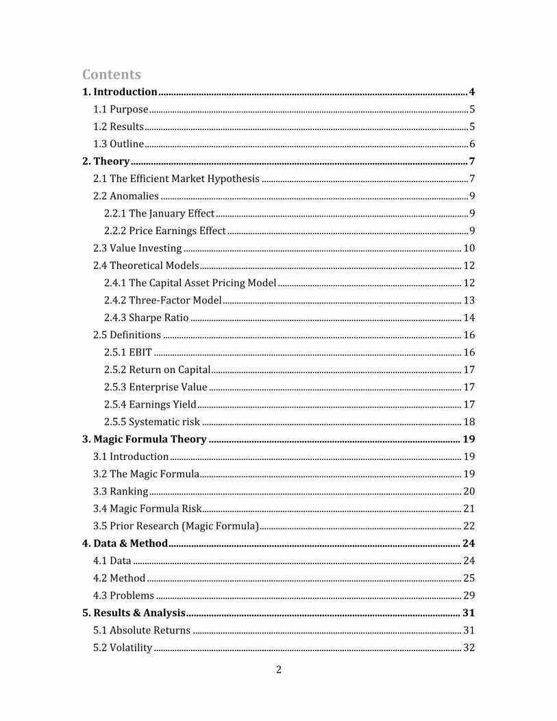
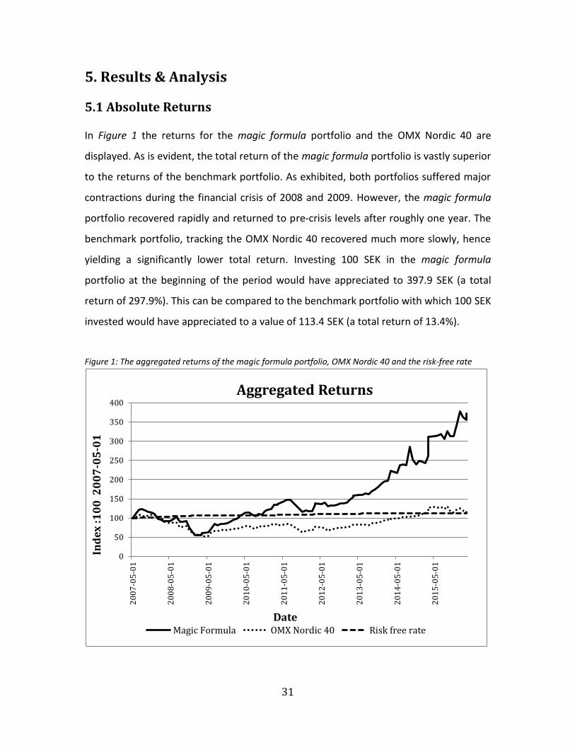
5.1 Absolute Returns In Figure 1 the returns for the magic formula portfolio and the OMX Nordic 40 are

displayed. As is evident, the total return of the magic formula portfolio is vastly superior

to the returns of the benchmark portfolio. As exhibited, both portfolios suffered major

contractions during the financial crisis of 2008 and 2009. However, the magic formula

portfolio recovered rapidly and returned to pre-crisis levels after roughly one year. The

benchmark portfolio, tracking the OMX Nordic 40 recovered much more slowly, hence

yielding a significantly lower total return. Investing 100 SEK in the magic formula

portfolio at the beginning of the period would have appreciated to 397.9 SEK (a total

return of 297.9%). This can be compared to the benchmark portfolio with which 100 SEK

invested would have appreciated to a value of 113.4 SEK (a total return of 13.4%).

Figure 1: The aggregated returns of the magic formula portfolio, OMX Nordic 40 and the risk-free rate

32

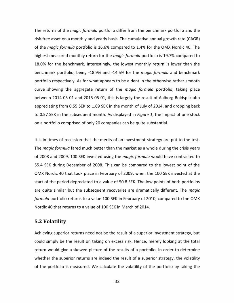
The returns of the magic formula portfolio differ from the benchmark portfolio and the

risk-free asset on a monthly and yearly basis. The cumulative annual growth rate (CAGR)

of the magic formula portfolio is 16.6% compared to 1.4% for the OMX Nordic 40. The

highest measured monthly return for the magic formula portfolio is 19.7% compared to

18.0% for the benchmark. Interestingly, the lowest monthly return is lower than the

benchmark portfolio, being -18.9% and -14.5% for the magic formula and benchmark

portfolio respectively. As for what appears to be a dent in the otherwise rather smooth

curve showing the aggregate return of the magic formula portfolio, taking place

between 2014-05-01 and 2015-05-01, this is largely the result of Aalborg Boldspilklubb

appreciating from 0.55 SEK to 1.69 SEK in the month of July of 2014, and dropping back

to 0.57 SEK in the subsequent month. As displayed in Figure 1, the impact of one stock

on a portfolio comprised of only 20 companies can be quite substantial.

It is in times of recession that the merits of an investment strategy are put to the test.

The magic formula fared much better than the market as a whole during the crisis years

of 2008 and 2009. 100 SEK invested using the magic formula would have contracted to

55.4 SEK during December of 2008. This can be compared to the lowest point of the

OMX Nordic 40 that took place in February of 2009, when the 100 SEK invested at the

start of the period depreciated to a value of 50.8 SEK. The low points of both portfolios

are quite similar but the subsequent recoveries are dramatically different. The magic

formula portfolio returns to a value 100 SEK in February of 2010, compared to the OMX

Nordic 40 that returns to a value of 100 SEK in March of 2014.

5.2 Volatility Achieving superior returns need not be the result of a superior investment strategy, but

could simply be the result on taking on excess risk. Hence, merely looking at the total

return would give a skewed picture of the results of a portfolio. In order to determine

whether the superior returns are indeed the result of a superior strategy, the volatility

of the portfolio is measured. We calculate the volatility of the portfolio by taking the

33

0,00%

1,00%

2,00%

3,00%

4,00%

5,00%

6,00%

7,00%

20

07

-05

-01

20

08

-05

-01

20

09

-05

-01

20

10

-05

-01

20

11

-05

-01

20

12

-05

-01

20

13

-05

-01

20

14

-05

-01

20

15

-05

-01

Vo

lati

lity

(σ

)

Date

Monthly Volatility

MAGIC FORMULA OMX Nordic 40

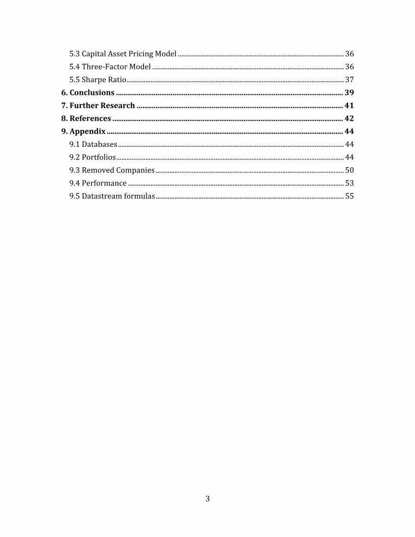
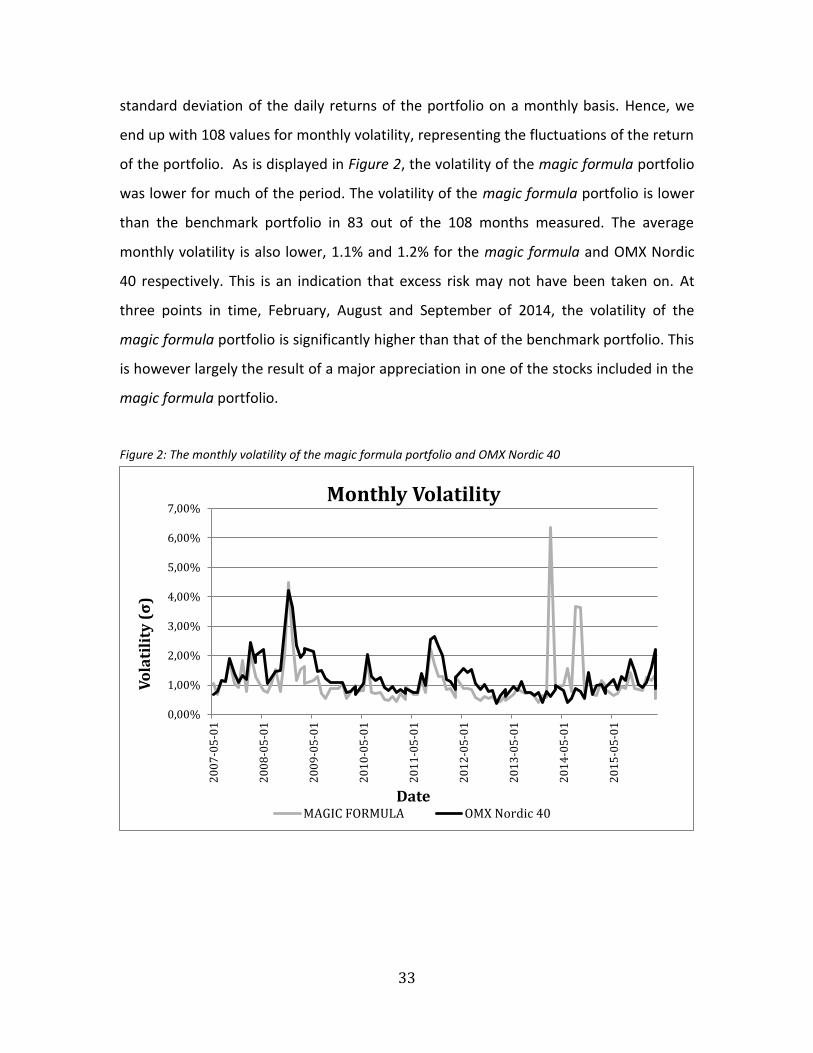
standard deviation of the daily returns of the portfolio on a monthly basis. Hence, we

end up with 108 values for monthly volatility, representing the fluctuations of the return

of the portfolio. As is displayed in Figure 2, the volatility of the magic formula portfolio

was lower for much of the period. The volatility of the magic formula portfolio is lower

than the benchmark portfolio in 83 out of the 108 months measured. The average

monthly volatility is also lower, 1.1% and 1.2% for the magic formula and OMX Nordic

40 respectively. This is an indication that excess risk may not have been taken on. At

three points in time, February, August and September of 2014, the volatility of the

magic formula portfolio is significantly higher than that of the benchmark portfolio. This

is however largely the result of a major appreciation in one of the stocks included in the

magic formula portfolio.

Figure 2: The monthly volatility of the magic formula portfolio and OMX Nordic 40

34

In the case of February of 2014, Nordic Shipbuilding appreciated from a value of 0.85

SEK to 2.4 SEK. In September of the same year, Aalborg Boldspilklub went from a value

of 1.69 SEK at the start of the month to 0.57 SEK at the end of the month. In the case of

Aalborg Boldspilklub it is notable that over the course of the entire holding period, the

stock price only depreciated 7.5%. However, in the individual month of September the

price of the stock fell substantially, resulting in high volatility. Figure 2 shows that in the

case of a portfolio comprised of only 20 companies, a sudden change in price of a single

stock can have a large impact on the entire portfolio.

Furthermore, it is in the interest of the investigation to determine the degree to which

the financial crisis of 2008 and 2009 affected the volatility of the magic formula

portfolio. During the financial crisis of 2008 and 2009, which we for the sake of

simplicity define as the period 2008-09-01 to 2009-09-01, the volatility of the magic

formula portfolio was lower in all but one month out of the total twelve months. During

the month of November of 2008, the volatility of both portfolios increased significantly,

with standard deviations of 4.50% and 4.22% for the magic formula portfolio and OMX

Nordic 40 portfolio respectively. This indicates that the magic formula does not

necessarily constitute a greater risk than the market as a whole during times of financial

crises.

In addition to standard deviation, the beta of the portfolio is also measured. Beta, being

a measure of how much an asset is exposed to market risk, indicating how much a

portfolio fluctuates in relation to the market, is used in order to determine if the magic

formula portfolio is indeed riskier than the benchmark portfolio. We calculate the

portfolio beta on a 36-month trailing basis. Hence, the beta of our portfolio is only

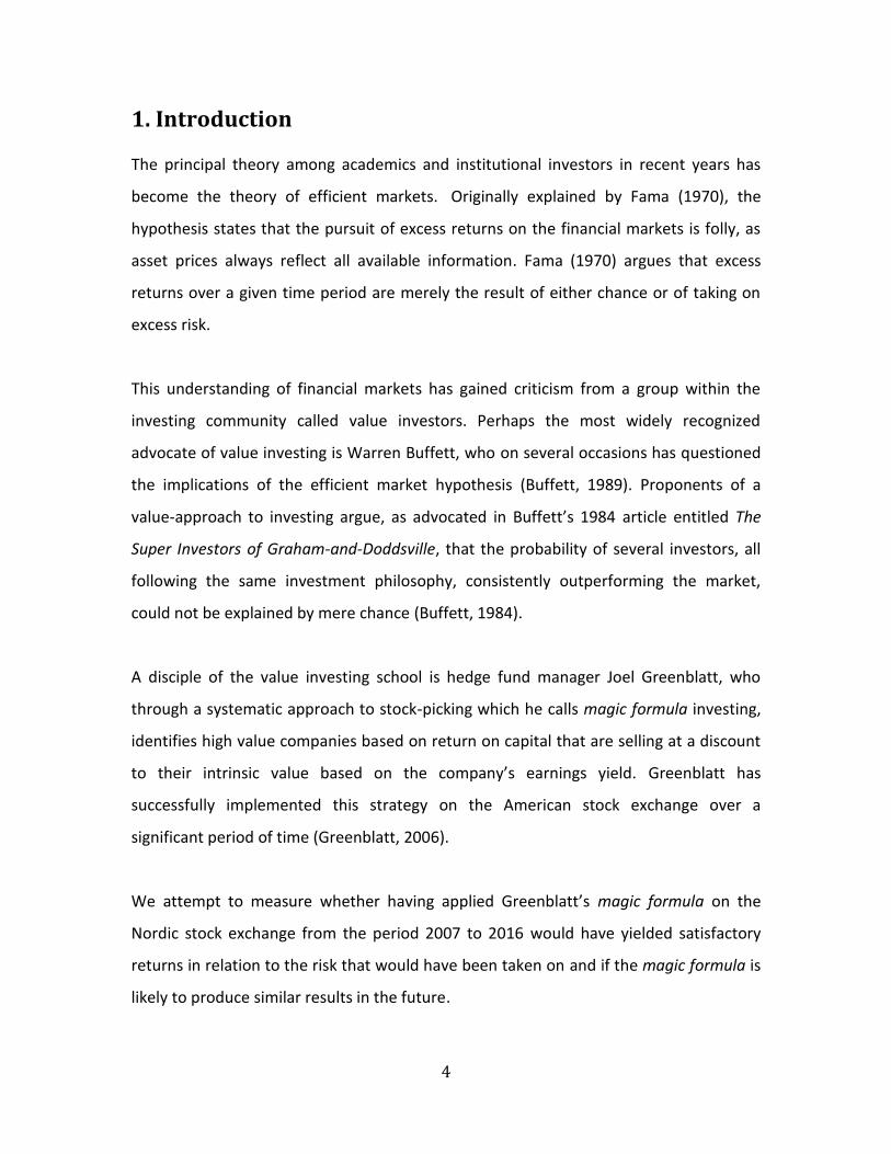
available three years into the testing period. The beta of the portfolio is significantly

lower than 1.0 for the entire period, with 0.43 and 0.62 being the lowest and highest

betas recorded (Figure 3, p.35). The magic formula portfolio exhibits an average beta for

the entire period of 0.54, indicating that the portfolio fluctuates less than the

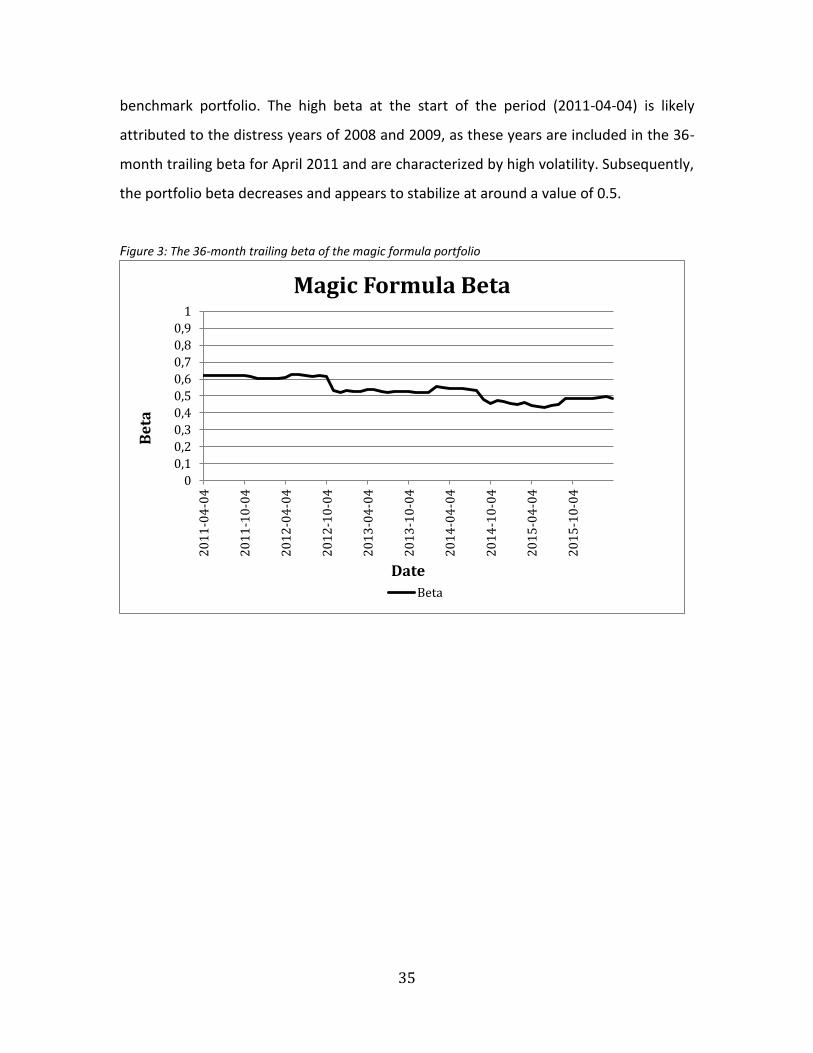
35

0

0,1

0,2

0,3

0,4

0,5

0,6

0,7

0,8

0,9

1

20

11

-04

-04

20

11

-10

-04

20

12

-04

-04

20

12

-10

-04

20

13

-04

-04

20

13

-10

-04

20

14

-04

-04

20

14

-10

-04

20

15

-04

-04

20

15

-10

-04

Be

ta

Date

Magic Formula Beta

Beta

benchmark portfolio. The high beta at the start of the period (2011-04-04) is likely

attributed to the distress years of 2008 and 2009, as these years are included in the 36-

month trailing beta for April 2011 and are characterized by high volatility. Subsequently,

the portfolio beta decreases and appears to stabilize at around a value of 0.5.

Figure 3: The 36-month trailing beta of the magic formula portfolio

36

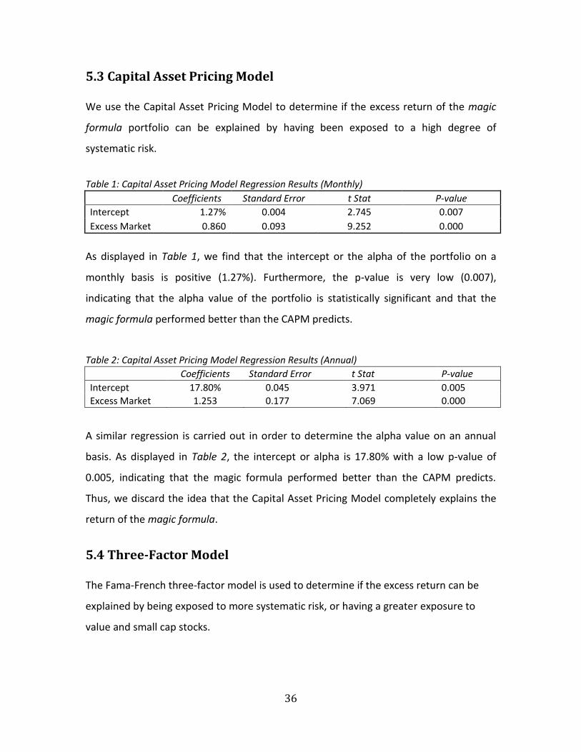
5.3 Capital Asset Pricing Model We use the Capital Asset Pricing Model to determine if the excess return of the magic

formula portfolio can be explained by having been exposed to a high degree of

systematic risk.

Table 1: Capital Asset Pricing Model Regression Results (Monthly)

Coefficients Standard Error t Stat P-value

Intercept 1.27% 0.004 2.745 0.007

Excess Market 0.860 0.093 9.252 0.000

As displayed in Table 1, we find that the intercept or the alpha of the portfolio on a

monthly basis is positive (1.27%). Furthermore, the p-value is very low (0.007),

indicating that the alpha value of the portfolio is statistically significant and that the

magic formula performed better than the CAPM predicts.

Table 2: Capital Asset Pricing Model Regression Results (Annual)


Intercept 17.80% 0.045 3.971 0.005

Excess Market 1.253 0.177 7.069 0.000

A similar regression is carried out in order to determine the alpha value on an annual

basis. As displayed in Table 2, the intercept or alpha is 17.80% with a low p-value of

0.005, indicating that the magic formula performed better than the CAPM predicts.

Thus, we discard the idea that the Capital Asset Pricing Model completely explains the

return of the magic formula.

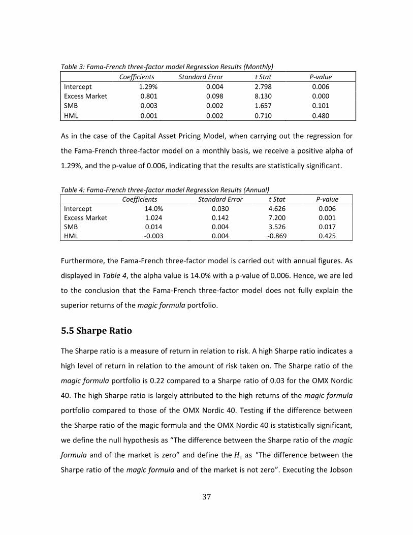
5.4 Three-Factor Model The Fama-French three-factor model is used to determine if the excess return can be

explained by being exposed to more systematic risk, or having a greater exposure to

value and small cap stocks.

37

Table 3: Fama-French three-factor model Regression Results (Monthly)


Intercept 1.29% 0.004 2.798 0.006

Excess Market 0.801 0.098 8.130 0.000

SMB 0.003 0.002 1.657 0.101

HML 0.001 0.002 0.710 0.480

As in the case of the Capital Asset Pricing Model, when carrying out the regression for

the Fama-French three-factor model on a monthly basis, we receive a positive alpha of

1.29%, and the p-value of 0.006, indicating that the results are statistically significant.

Table 4: Fama-French three-factor model Regression Results (Annual)


Intercept 14.0% 0.030 4.626 0.006 Excess Market 1.024 0.142 7.200 0.001 SMB 0.014 0.004 3.526 0.017 HML -0.003 0.004 -0.869 0.425

Furthermore, the Fama-French three-factor model is carried out with annual figures. As

displayed in Table 4, the alpha value is 14.0% with a p-value of 0.006. Hence, we are led

to the conclusion that the Fama-French three-factor model does not fully explain the

superior returns of the magic formula portfolio.

5.5 Sharpe Ratio The Sharpe ratio is a measure of return in relation to risk. A high Sharpe ratio indicates a

high level of return in relation to the amount of risk taken on. The Sharpe ratio of the

magic formula portfolio is 0.22 compared to a Sharpe ratio of 0.03 for the OMX Nordic

40. The high Sharpe ratio is largely attributed to the high returns of the magic formula

portfolio compared to those of the OMX Nordic 40. Testing if the difference between

the Sharpe ratio of the magic formula and the OMX Nordic 40 is statistically significant,

we define the null hypothesis as “The difference between the Sharpe ratio of the magic

formula and of the market is zero” and define the 𝐻1 as “The difference between the

Sharpe ratio of the magic formula and of the market is not zero”. Executing the Jobson

38

and Korkie (1981) procedure and carrying out a two-sided t-test we receive a p-value of

0.018. The p-value of the test is lower than 0.05, which is the customary level of

significance, indicating that the results are statistically significant. We therefore reject

the null hypothesis and conclude that the difference between the Sharpe ratio of the

magic formula and of the market is not zero. Hence, the high Sharpe ratio of the magic

formula portfolio cannot be attributed to luck or chance.

39

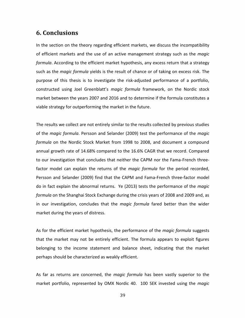
6. Conclusions In the section on the theory regarding efficient markets, we discuss the incompatibility

of efficient markets and the use of an active management strategy such as the magic

formula. According to the efficient market hypothesis, any excess return that a strategy

such as the magic formula yields is the result of chance or of taking on excess risk. The

purpose of this thesis is to investigate the risk-adjusted performance of a portfolio,

constructed using Joel Greenblatt’s magic formula framework, on the Nordic stock

market between the years 2007 and 2016 and to determine if the formula constitutes a

viable strategy for outperforming the market in the future.

The results we collect are not entirely similar to the results collected by previous studies

of the magic formula. Persson and Selander (2009) test the performance of the magic

formula on the Nordic Stock Market from 1998 to 2008, and document a compound

annual growth rate of 14.68% compared to the 16.6% CAGR that we record. Compared

to our investigation that concludes that neither the CAPM nor the Fama-French three-

factor model can explain the returns of the magic formula for the period recorded,

Persson and Selander (2009) find that the CAPM and Fama-French three-factor model

do in fact explain the abnormal returns. Ye (2013) tests the performance of the magic

formula on the Shanghai Stock Exchange during the crisis years of 2008 and 2009 and, as

in our investigation, concludes that the magic formula fared better than the wider

market during the years of distress.

As for the efficient market hypothesis, the performance of the magic formula suggests

that the market may not be entirely efficient. The formula appears to exploit figures

belonging to the income statement and balance sheet, indicating that the market

perhaps should be characterized as weakly efficient.

As far as returns are concerned, the magic formula has been vastly superior to the

market portfolio, represented by OMX Nordic 40. 100 SEK invested using the magic

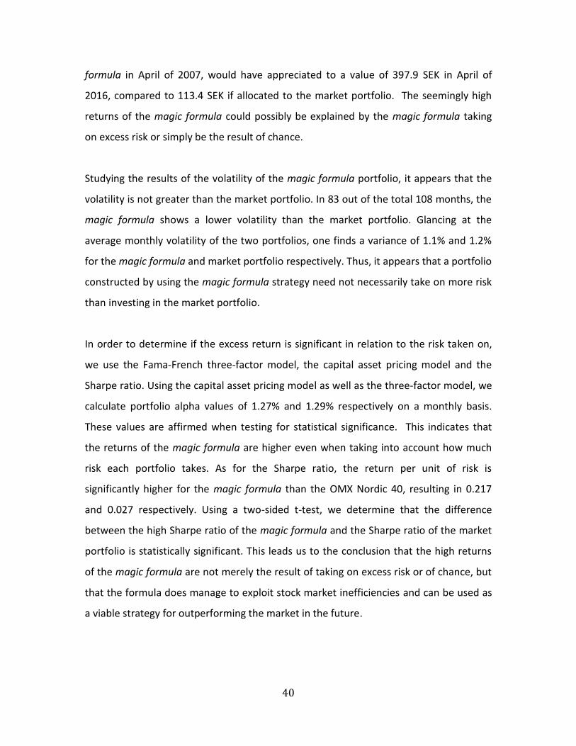
40

formula in April of 2007, would have appreciated to a value of 397.9 SEK in April of

2016, compared to 113.4 SEK if allocated to the market portfolio. The seemingly high

returns of the magic formula could possibly be explained by the magic formula taking

on excess risk or simply be the result of chance.

Studying the results of the volatility of the magic formula portfolio, it appears that the

volatility is not greater than the market portfolio. In 83 out of the total 108 months, the

magic formula shows a lower volatility than the market portfolio. Glancing at the

average monthly volatility of the two portfolios, one finds a variance of 1.1% and 1.2%

for the magic formula and market portfolio respectively. Thus, it appears that a portfolio

constructed by using the magic formula strategy need not necessarily take on more risk

than investing in the market portfolio.

In order to determine if the excess return is significant in relation to the risk taken on,

we use the Fama-French three-factor model, the capital asset pricing model and the

Sharpe ratio. Using the capital asset pricing model as well as the three-factor model, we

calculate portfolio alpha values of 1.27% and 1.29% respectively on a monthly basis.

These values are affirmed when testing for statistical significance. This indicates that

the returns of the magic formula are higher even when taking into account how much

risk each portfolio takes. As for the Sharpe ratio, the return per unit of risk is

significantly higher for the magic formula than the OMX Nordic 40, resulting in 0.217

and 0.027 respectively. Using a two-sided t-test, we determine that the difference

between the high Sharpe ratio of the magic formula and the Sharpe ratio of the market

portfolio is statistically significant. This leads us to the conclusion that the high returns

of the magic formula are not merely the result of taking on excess risk or of chance, but

that the formula does manage to exploit stock market inefficiencies and can be used as

a viable strategy for outperforming the market in the future.

41

7. Further Research Modern portfolio theory is largely absent from the magic formula, perhaps to its

advantage. A suggestion for further research would be to incorporate modern portfolio

theory to Greenblatt’s strategy. One such suggestion would be to research the effect of

assigning a greater weight to either the return on capital component or the earnings

yield component of the formula. As opposed to giving the same weight to both the

quality and valuation component, perhaps an optimum weight for each measure could

be identified.

Following Greenblatt’s strategy, each stock in the magic formula portfolio is assigned

the same weight. In other words, a portfolio consisting of 20 companies would allocate

5 percent of the total capital to each stock, irrespective of ranking. It would perhaps be

in the interest of future researchers to investigate if a greater proportion of the total

capital should be allocated to the companies with higher rankings. An optimum weight

corresponding to the overall ranking could perhaps be calculated.

42

8. References

Basu, S (1977), “Investment performance of common stocks in relation to their price earnings ratios: A test of market efficiency”, Journal of Finance, Vol. 32, pp.663-682.

Bodie, Z., Kane, A. & Marcus, A.J., (2014), “Investments”, 10th edn, Berkshire, McGraw-Hill. Buffett, W (1984-05-17), “The Superinvestors of Graham-and-Doddsville”, Columbia Business School, Available Online:https://www8.gsb.columbia.edu/articles/columbia-business/superinvestors [Accessed 12 December 2016] Buffett, W (1989-02-28), “Berkshire Hathaway Shareholder Letters 1988”, Available Online: http://berkshirehathaway.com/letters/1988.html [Accessed 19 December 2016] Buffett, W (1994-03-01), “Berkshire Hathaway Shareholder Letters 1993”, Available Online: http://berkshirehathaway.com/letters/1993.html [Accessed 19 December 2016] Buffett, W (2009-02-27), “Berkshire Hathaway Shareholder Letters 2008”, Available Online: http://www.berkshirehathaway.com/letters/2008ltr.pdf [Accessed 19 December 2016]

Cochrane, J. H. (1999), "New Facts in Finance”, Economic Perspectives Federal Reserve Bank of Chicago, Issue Q III, pp.36-58.

Fama, E (1970), “Efficient Capital Markets: A Review of Theory and Empirical Work”, Journal of Finance, Vol. 25, pp.383–417.

Fama, E & French, K.R. (1993), “Common Risk Factors in the Returns on Stocks and Bonds”, Journal of Financial Economics, Vol. 33, pp.3–56.

Graham, B & Dodd, D (1934), “Security Analysis”, 1st edn, New York, McGraw-Hill.

Graham, B & Dodd, D (2009), “Security Analysis”, 6th edn, New York, McGraw-Hill, pp.669.

Greenblatt, J (2006), “The Little Book That Beats the Market”, Hoboken, John Wiley & Sons Inc.

Jobson, J. D. & Korkie, B. M. (1981), “Performance Hypothesis Testing with the Sharpe and Treynor Measures”, The Journal of Finance, Vol. 36, pp.889-908.

https://www8.gsb.columbia.edu/articles/columbia-business/superinvestors

https://www8.gsb.columbia.edu/articles/columbia-business/superinvestors

http://berkshirehathaway.com/letters/1988.html

http://berkshirehathaway.com/letters/1993.html

http://www.berkshirehathaway.com/letters/2008ltr.pdf

43

NASDAQ (2017), ”OMX Nordic 40” Available Online: https://indexes.nasdaqomx.com/Index/Overview/OMXN40 [Accessed 2 January 2017]

Persson, V & Selander, N (2009), “Back testing “The Magic Formula” in the Nordic region”, Master Thesis, Stockholm School of Economics, Available Online: http://arc.hhs.se/download.aspx?MediumId=769 [Accessed 15 November 2016]

Read, C (1898), “Logic, Deductive and Inductive”, Ballantyne, Hanson and Co, pp.272.

Rozeff, M. S. & Kinney, W (1976), “Capital market seasonality: The case of stock returns”, Journal of Financial Economics, Vol. 3, pp.379-402.

Sharpe, W. F. (1994), “The Sharpe Ratio”, Journal of Portfolio Management, Vol. 21, pp.49–58.

Wachtel, S. B. (1942), “Certain observations on seasonal movements in stock prices”, Journal of Business, Vol. 15, pp.184-193.

Womack, K. L. & Zhang, Y (2003), “Understanding Risk and Return, the CAPM, and the Fama-French Three-Factor Model”, Tuck Case No. 03-111.

Ye, Y (2013), “Application of the Stock Selection Criteria of Three Value Investors, Benjamin Graham, Peter Lynch, and Joel Greenblatt: A Case of Shanghai Stock Exchange from 2006 to 2011”, International Journal of Scientific and Research Publications, Vol. 3 Issue 8.

https://indexes.nasdaqomx.com/Index/Overview/OMXN40

http://arc.hhs.se/download.aspx?MediumId=769

44

9. Appendix

9.1 Databases

Bloomberg Terminal

Kenneth French “Data Library” Available Online: http://mba.tuck.dartmouth.edu/pages/faculty/ken.french/data_library.html [Accessed 15 December 2016]

NASDAQ OMX Nordic http://www.nasdaqomxnordic.com/ [Accessed 28 November 2016] The Swedish Riksbank’s database of Market rates, Available Online: http://www.riksbank.se/sv/Rantor-och-valutakurser/Sok-rantor-och-valutakurser/ [Accessed 7 December 2016]

Thomson Reuters Datastream

9.2 Portfolios

2007-03-30 – 2008-03-31

BE GROUP AB

BEIJER ALMA AB

BERGS TIMBER AB

BOLIDEN AB

DAMPSKIBS NORDEN AS

JEEVES INFORMATION

KABE HUSVAGNAR AB

KNOWIT AB

KONECRANES ABP

NCC AB

NORDIC ALUMINIUM OYJ

RAUTARUUKKI CORP

RAUTE OYJ

RORVIK TIMBER AB

SCHOUW & CO A/S

SOFTRONIC AB

SPAENCOM A/S

TICKET TRAVEL GROUP

http://mba.tuck.dartmouth.edu/pages/faculty/ken.french/data_library.html

http://www.nasdaqomxnordic.com/

http://www.riksbank.se/sv/Rantor-och-valutakurser/Sok-rantor-och-valutakurser/

45

TORM PLC

UNIFLEX AB

2008-04-01 – 2009-03-31

ACANDO AB

BE GROUP AB

BIOTAGE AB

DAMPSKIBS NORDEN AS

HIQ INTERNATIONAL AB

HOJGAARD HOLDING A/S

JEEVES INFORMATION

KNOWIT AB

KONECRANES ABP

MARTELA OYJ

MODERN TIMES GRP

OUTOTEC OYJ

POOLIA AB

POYRY OYJ

PREVAS AB

REJLERS PUBL AB

SOFTRONIC AB

SWECO AB

TEKLA OYJ

UNIFLEX AB

2009-04-01 – 2010-03-31

ABB LTD

ADDTECH AB

ASTRAZENECA PLC

AXFOOD AB

DORO AB

EXEL COMPOSITES OYJ

FLSMIDTH & CO A/S

H. LUNDBECK A/S

HOJGAARD HOLDING A/S

MILLICOM INTERNATIO

NETONNET AB

ORC GROUP

ORION OYJ

PROACT IT GROUP AB

Q-MED AB

46

SKANSKA AB

SOFTRONIC AB

UNITED INTERNATIONAL

U-SEA BULK SHIP

WARTSILA OYJ

2010-04-01 – 2011-03-31

AF AB

ASTRAZENECA PLC

ATLANTIC PETROLEUM

AVAILO PUBL AB

AVEGA GROUP AB

BETSSON AB

DORO AB

DOVRE GROUP

GN STORE NORD A/S

H. LUNDBECK A/S

KABE HUSVAGNAR AB

KARJALAN KIRJAPAINO

LUNDIN PETROLEUM AB

MILLICOM INTERNATIO

NORDIC ALUMINIUM OYJ

ODD MOLLY INTERNA

ORION OYJ

SANTA FE GROUP A/S

TELE2 AB

UNIFLEX AB

2011-04-01 – 2012-03-30

ASPOCOMP GROUP OYJ

ASTRAZENECA PLC

AVAILO PUBL AB

AVEGA GROUP AB

BILIA AB

CBRAIN A/S

COMPTEL OYJ

DORO AB

EWORK GROUP AB

HALDEX AB

HOLMEN AB

JEEVES INFORMATION

47

MALMBERGS ELEKTRISKA

MICRO SYSTEMATION AB

NORTH MEDIA AS

ORION OYJ

PANDORA

PROFFICE AB

SAAB AB

UNIFLEX AB

2012-03-30 – 2013-03-29

ASTRAZENECA PLC

BIOGAIA AB

DEDICARE AB

ENEA AB

ENQUEST PLC

EWORK GROUP AB

FISKARS OYJ

GLUNZ & JENSEN HOL

HAGAR HF

KABE HUSVAGNAR AB

KOEBENHAVNS

LAGERCRANTZ GROUP AB

METSA BOARD OYJ

MODERN TIMES GRP

ROBLON AS

SAGA FURS OYJ

SECTRA AB

SEMCON AB


VENUE RETAIL GROUP

2013-04-01 – 2014-03-31

ALLTELE ALLMANNA SVE

AVEGA GROUP AB

DEDICARE AB

DOVRE GROUP

ELECTRA GRUPPEN AB

ENEA AB

ENQUEST PLC

F-SECURE OYJ

HAGAR HF

48

ICA GRUPPEN AB

ICELANDAIR GROUP

LAGERCRANTZ GROUP AB

MALMBERGS ELEKTRISKA

NOLATO AB

NORDIC SHIP

NOVOTEK AB

ORION OYJ

SWEDISH MATCH AB


VBG GROUP AB

2014-04-01 – 2015-03-31

AALBORG BOLDSPILKLUB

AVEGA GROUP AB

COLUMBUS A/S

DEDICARE AB

FISKARS OYJ

HAGAR HF

LUCARA DIAMOND

MEDIVIR AB

MILLICOM INTERNATIO

MULTIQ INTL AB

MYCRONIC AB

NOLATO AB

NORDIC MINES AB

NOVOTEK AB

PONSSE OYJ

QPR SOFTWARE OYJ

ROTTNEROS AB

RTX TELECOM A/S

SCANDINAVIAN BRAKE

TETHYS

2015-04-01 – 2016-03-31

AVEGA GROUP AB

BILIA AB

COLUMBUS A/S

CONCENTRIC AB

DEDICARE AB

HAGAR HF

49

ICELANDAIR GROUP

KONE CORPORATION

LUCARA DIAMOND

NOKIA CORP

NOLATO AB

NOVOTEK AB

PONSSE OYJ

POOLIA AB

RAUTE OYJ

RNB RETAIL

ROTTNEROS AB

TRAINERS HOUSE

UNIFLEX AB

YLEISELEKTRONIIKKA

50

9.3 Removed Companies

Companies removed due to being classified as utilities or financials or due to a lack of

data.

A/S GRONLANDSBANKEN

A/S MONS BANK

ADMIRAL CAPITAL A/S

AKTIA BANK PLC

ALANDSBANKEN ABP

ALM. BRAND A/S

ARISE AB

ASIAKASTIETO

ATRIUM LJUNGBERG AB

AVANZA BANK

BANKNORDIK P/F

BESQAB AB (PUBL)

BLUE VISION

BONAVA AB

BURE EQUITY AB

CAPMAN OYJ

CASTELLUM AB

CATENA AB

CITYCON OYJ

COLLECTOR AB

COREM PROPERTY

DANSKE A

DANSKE BANK A/S

DIOS FASTIGHETER

DJURSLANDS BANK A/S

DONG ENERGY A/S

EAST CAPITAL

EIK FASTE

EQ OYJ

ETRION CORP

EVLI PANKKI OYJ

F E BORDING A/S

FABEGE AB

FASTIGHETS AB BALDER

FASTPARTNER AB

FORTUM OYJ

FYNSKE BANK

GERMAN HIGH STREET P

51

GREENTECH ENGERY

HEBA FASTIGHETS AB

HEMFOSA FASTIGHETER

HUFVUDSTADEN AB

HVIDBJERG BANK A/S

INDUSTRIVARDEN AB

INTRUM JUSTITIA AB

INVEST LUXOR AS

INVESTMENT AB LATOUR

INVESTOR AB

INVESTORS HOUSE OYJ

JEUDAN A/S

JM AB

JUTLANDER BANK

JYSKE BANK A/S

KINNEVIK

KLOVERN AB

KREDITBANKEN AS

KUNGSLEDEN AB

L E LUNDBERGFORET

LAN & SPAR BANK A/S

MELKER SCHORLING AB

MIDWAY HOLDING AB

NEWCAP HOLDING A/S

NGS NEXT GENERATION

NORDAX GROUP

NORDEA BANK

NORDFYNS BANK A/S

NORDICOM A/S

NORDJYSKE BANK AS

NORDNET SECURITIES

NP3 FASTIGHETER AB

ORAVA ASUNTORAH

ORESUND INVESTMENT

OSCAR PROPERTIES

OSTJYDSK BANK A/S

PANDOX AB

PANOSTAJA OYJ

PLATZER FASTIGHETER

PRIME OFFICE

RATOS AB

REGINN HF

REITIR FASTEIGNA

52

RESURS HOLDING AB

RINGKJ. LANDBOBANK

SAGAX AB

SALLING BANK A/S

SAMPO OYJ

SIEVI CAPITAL OYJ

SJOVA-ALMENNAR

SKANDINAVISKA ENSK

SKJERN BANK A/S

SPAR NORD BANK

SPAREKASSEN

SPONDA OYJ

STRATEGIC INV

STRAX

SV. HANDELSBANKEN AB

SWEDBANK AB

SYDBANK A/S

TAALERI OYJ

TECHNOPOLIS OYJ

TF BANK

TK DEVELOPMENT A/S

TOPDANMARK A/S

TOTALBANKEN A/S

TRACTION AB

TRYG A/S

WALLENSTAM AB

VESTJYSK BANK A/S

VICTORIA PARK I

VICTORIA PROPERTIES

VIS INSURANCE LTD

VOSTOK NEW

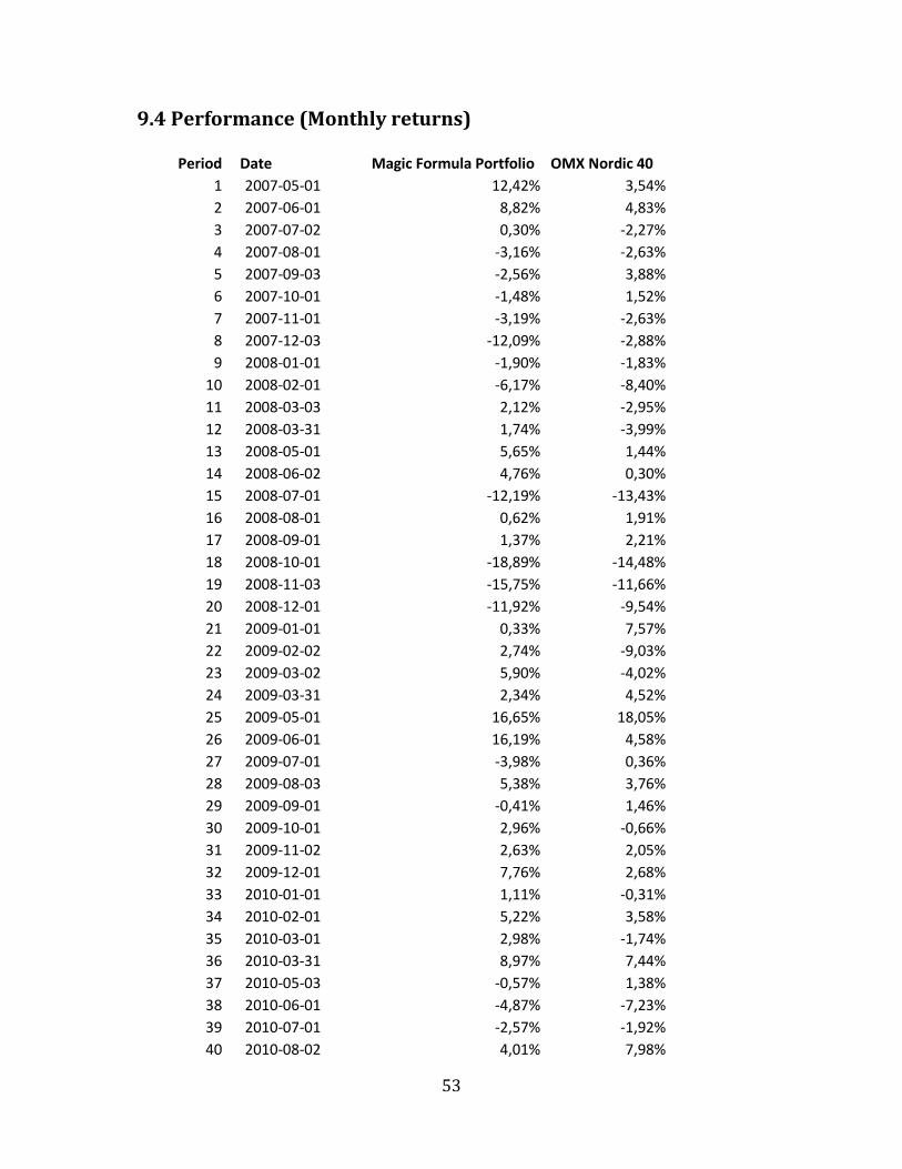
53

9.4 Performance (Monthly returns)

Period Date Magic Formula Portfolio OMX Nordic 40

1 2007-05-01 12,42% 3,54%

2 2007-06-01 8,82% 4,83%

3 2007-07-02 0,30% -2,27%

4 2007-08-01 -3,16% -2,63%

5 2007-09-03 -2,56% 3,88%

6 2007-10-01 -1,48% 1,52%

7 2007-11-01 -3,19% -2,63%

8 2007-12-03 -12,09% -2,88%

9 2008-01-01 -1,90% -1,83%

10 2008-02-01 -6,17% -8,40%

11 2008-03-03 2,12% -2,95%

12 2008-03-31 1,74% -3,99%

13 2008-05-01 5,65% 1,44%

14 2008-06-02 4,76% 0,30%

15 2008-07-01 -12,19% -13,43%

16 2008-08-01 0,62% 1,91%

17 2008-09-01 1,37% 2,21%

18 2008-10-01 -18,89% -14,48%

19 2008-11-03 -15,75% -11,66%

20 2008-12-01 -11,92% -9,54%

21 2009-01-01 0,33% 7,57%

22 2009-02-02 2,74% -9,03%

23 2009-03-02 5,90% -4,02%

24 2009-03-31 2,34% 4,52%

25 2009-05-01 16,65% 18,05%

26 2009-06-01 16,19% 4,58%

27 2009-07-01 -3,98% 0,36%

28 2009-08-03 5,38% 3,76%

29 2009-09-01 -0,41% 1,46%

30 2009-10-01 2,96% -0,66%

31 2009-11-02 2,63% 2,05%

32 2009-12-01 7,76% 2,68%

33 2010-01-01 1,11% -0,31%

34 2010-02-01 5,22% 3,58%

35 2010-03-01 2,98% -1,74%

36 2010-03-31 8,97% 7,44%

37 2010-05-03 -0,57% 1,38%

38 2010-06-01 -4,87% -7,23%

39 2010-07-01 -2,57% -1,92%

40 2010-08-02 4,01% 7,98%

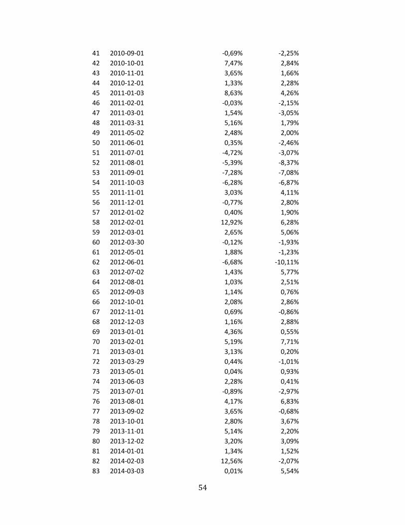
54

41 2010-09-01 -0,69% -2,25%

42 2010-10-01 7,47% 2,84%

43 2010-11-01 3,65% 1,66%

44 2010-12-01 1,33% 2,28%

45 2011-01-03 8,63% 4,26%

46 2011-02-01 -0,03% -2,15%

47 2011-03-01 1,54% -3,05%

48 2011-03-31 5,16% 1,79%

49 2011-05-02 2,48% 2,00%

50 2011-06-01 0,35% -2,46%

51 2011-07-01 -4,72% -3,07%

52 2011-08-01 -5,39% -8,37%

53 2011-09-01 -7,28% -7,08%

54 2011-10-03 -6,28% -6,87%

55 2011-11-01 3,03% 4,11%

56 2011-12-01 -0,77% 2,80%

57 2012-01-02 0,40% 1,90%

58 2012-02-01 12,92% 6,28%

59 2012-03-01 2,65% 5,06%

60 2012-03-30 -0,12% -1,93%

61 2012-05-01 1,88% -1,23%

62 2012-06-01 -6,68% -10,11%

63 2012-07-02 1,43% 5,77%

64 2012-08-01 1,03% 2,51%

65 2012-09-03 1,14% 0,76%

66 2012-10-01 2,08% 2,86%

67 2012-11-01 0,69% -0,86%

68 2012-12-03 1,16% 2,88%

69 2013-01-01 4,36% 0,55%

70 2013-02-01 5,19% 7,71%

71 2013-03-01 3,13% 0,20%

72 2013-03-29 0,44% -1,01%

73 2013-05-01 0,04% 0,93%

74 2013-06-03 2,28% 0,41%

75 2013-07-01 -0,89% -2,97%

76 2013-08-01 4,17% 6,83%

77 2013-09-02 3,65% -0,68%

78 2013-10-01 2,80% 3,67%

79 2013-11-01 5,14% 2,20%

80 2013-12-02 3,20% 3,09%

81 2014-01-01 1,34% 1,52%

82 2014-02-03 12,56% -2,07%

83 2014-03-03 0,01% 5,54%

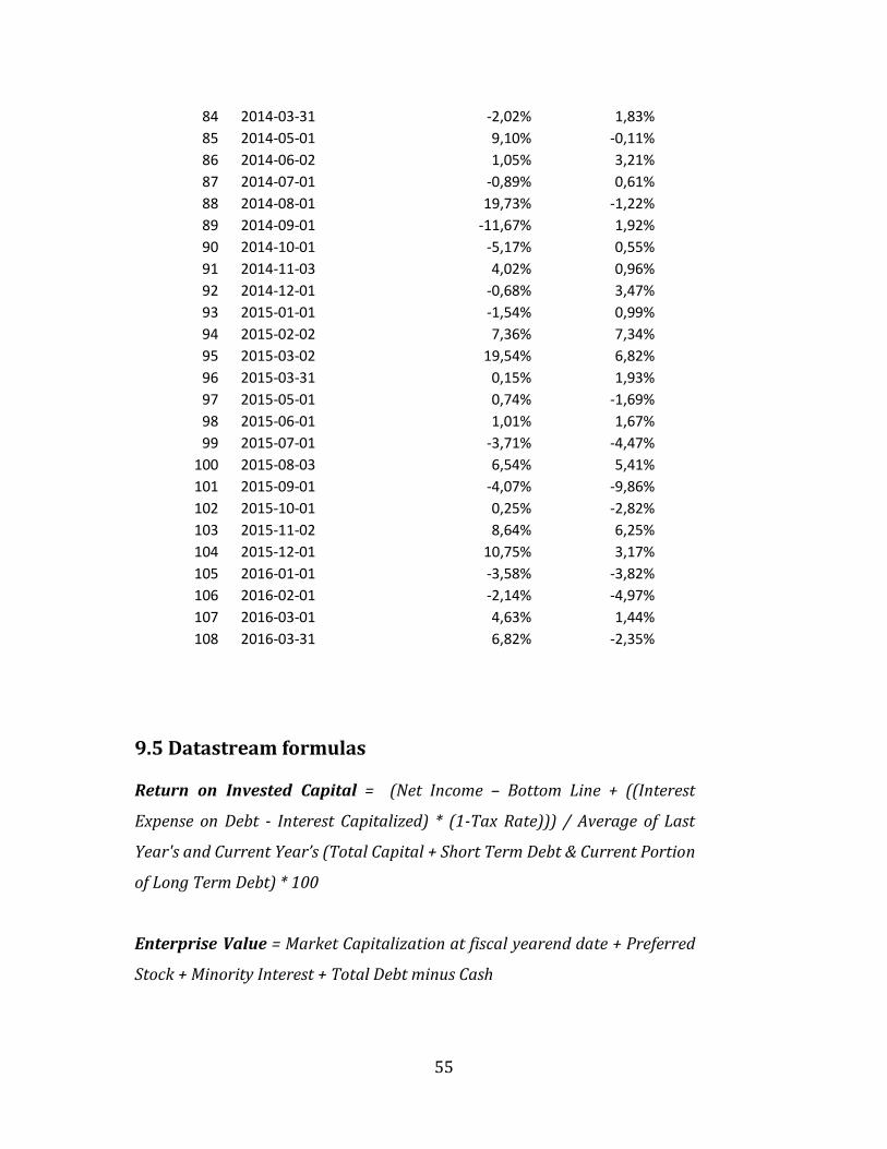
55

84 2014-03-31 -2,02% 1,83%

85 2014-05-01 9,10% -0,11%

86 2014-06-02 1,05% 3,21%

87 2014-07-01 -0,89% 0,61%

88 2014-08-01 19,73% -1,22%

89 2014-09-01 -11,67% 1,92%

90 2014-10-01 -5,17% 0,55%

91 2014-11-03 4,02% 0,96%

92 2014-12-01 -0,68% 3,47%

93 2015-01-01 -1,54% 0,99%

94 2015-02-02 7,36% 7,34%

95 2015-03-02 19,54% 6,82%

96 2015-03-31 0,15% 1,93%

97 2015-05-01 0,74% -1,69%

98 2015-06-01 1,01% 1,67%

99 2015-07-01 -3,71% -4,47%

100 2015-08-03 6,54% 5,41%

101 2015-09-01 -4,07% -9,86%

102 2015-10-01 0,25% -2,82%

103 2015-11-02 8,64% 6,25%

104 2015-12-01 10,75% 3,17%

105 2016-01-01 -3,58% -3,82%

106 2016-02-01 -2,14% -4,97%

107 2016-03-01 4,63% 1,44%

108 2016-03-31 6,82% -2,35%

9.5 Datastream formulas

Return on Invested Capital = (Net Income – Bottom Line + ((Interest

Expense on Debt - Interest Capitalized) * (1-Tax Rate))) / Average of Last

Year's and Current Year’s (Total Capital + Short Term Debt & Current Portion

of Long Term Debt) * 100

Enterprise Value = Market Capitalization at fiscal yearend date + Preferred

Stock + Minority Interest + Total Debt minus Cash

value investing on the nordic stock market - lund...

Documents