valuing ecosystem services as productive...
TRANSCRIPT
VALUING ECOSYSTEM SERVICES 179
Economic Policy January 2007 pp. 177–229 Printed in Great Britain© CEPR, CES, MSH, 2007.
Valuing ecosystem services as productive inputs
Edward B. Barbier
University of Wyoming
1. INTRODUCTION
Global concern over the disappearance of natural ecosystems and habitats hasprompted policymakers to consider the ‘value of ecosystem services’ in environmentalmanagement decisions. These ‘services’ are broadly defined as ‘the benefits peopleobtain from ecosystems’ (Millennium Ecosystem Assessment, 2003, p. 53).
However, our current understanding of key ecological and economic relationshipsis sufficient to value only a handful of ecological services. An important objective ofthis paper is to explain and illustrate through numerical examples the difficultiesfaced in valuing natural ecosystems and their services, compared to ordinary economicor financial assets. Specifically, the paper addresses the following three questions:
1. What progress has been made in valuing ecological services for policy analysis?2. What are the unique measurement issues that need to be overcome?3. How can future progress improve upon the shortcomings in existing methods?
I am grateful to David Aadland, Carlo Favero, Geoff Heal, Omer Moav and three anonymous referees for helpful comments.
The Managing Editor in charge of this paper was Paul Seabright.
180 EDWARD B. BARBIER
1.1. Key challenges and policy context
As a report from the US National Academy of Science has emphasized, ‘the fundamentalchallenge of valuing ecosystem services lies in providing an explicit description andadequate assessment of the links between the structure and functions of natural systems,the benefits (i.e., goods and services) derived by humanity, and their subsequent values’(Heal
et al.
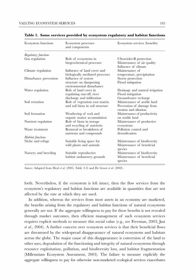
, 2005, p. 2). Moreover, it has been increasingly recognized by economistsand ecologists that the greatest ‘challenge’ they face is in valuing the ecosystemservices provided by a certain class of key ecosystem functions – regulatory and habitatfunctions. The diverse benefits of these functions include climate stability, maintenanceof biodiversity and beneficial species, erosion control, flood mitigation, storm protection,groundwater recharge and pollution control (see Table 1 below).
One of the natural ecosystems that has seen extensive development and applicationof methods to value ecosystem services has been coastal wetlands. This paper focusesmainly on valuation approaches applied to these systems, and in particular their roleas a nursery and breeding habitat for near-shore fisheries and in providing stormprotection for coastal communities.
The paper employs a case study of mangrove ecosystems in Thailand to compareand contrast approaches to valuing habitat and storm protection services. Globalmangrove area has been declining rapidly, with around 35% of the total area lost inthe past two decades (Valiela
et al.
, 2001). Mangrove deforestation has been particularlyprevalent in Thailand and other Asian countries. The main cause of global mangroveloss has been coastal economic development, especially aquaculture expansion(Barbier and Cox, 2003). Yet ecologists maintain that global mangrove loss is contributingto the decline of marine fisheries and leaving many coastal areas vulnerable tonatural disasters. Concern about the deteriorating ‘storm protection’ service ofmangroves reached new significance with the 26 December 2004 Asian tsunami thatcaused widespread devastation and loss of life in Thailand and other Indian Oceancountries.
The Thailand case study also illustrates the importance of valuing ecosystemservices to policy choices. Because these services are ‘non-marketed’, their benefitsare not considered in commercial development decisions. For example, the excessivemangrove deforestation occurring in Thailand and other countries is clearly relatedto the failure to measure explicitly the values of habitat and storm protection servicesof mangroves. Consequently, these benefits have been largely ignored in national landuse policy decisions, and calls to improve protection of remaining mangrove forestsand to enlist the support of local coastal communities through legal recognition oftheir
de facto
property rights over mangroves are unlikely to succeed in the face ofcoastal development pressures on these resources (Barbier and Sathirathai, 2004).Unless the value to local coastal communities of the ecosystem services provided byprotected mangroves is estimated, it is difficult to convince policymakers in Thailandand other countries to consider alternative land use policies.
VALUING ECOSYSTEM SERVICES 181
Thus, as the Thailand case study reveals, the challenge of valuing ecosystemservices is also a policy challenge. Because the benefits of these services are importantand should be taken into account in any future policy to manage coastal wetlands inThailand and other countries, it is equally essential that economics continues todevelop and improve existing methodologies to value ecological services.
1.2. Outline and main results
The paper makes three contributions. The first is to demonstrate that valuing eco-logical services as productive inputs is a viable methodology for policy analysis, andto illustrate the key steps through a detailed case study of mangroves in Thailand.The second contribution is to identify the measurement issues that make valuation ofnon-marketed ecosystem services a unique challenge, yet one that is important formany important policy decisions concerning the management of natural ecosystems.The third contribution of the paper is to show, using the examples of habitat andstorm protection services, that improvements in methods for valuing these servicescan correct for some shortcomings and measurement errors, thus yielding more accu-rate valuation estimates. But even the preferred approaches display measurementweaknesses that need to be addressed in future developments of ecosystem valuationmethodologies.
Section 2 discusses in more detail the importance of valuing ecosystem services,especially those arising from the regulatory and habitat functions to environmentaldecision-making. Section 3 reviews various methods for valuing these services.Because the benefits arising from ecological regulatory and habitat functions mainlysupport or protect valuable economic activities, the production function (PF)approach of valuing these benefits as environmental inputs is a promising methodology.However, the latter approach faces its own unique measurement issues. To illus-trate the PF approach as well as its shortcomings, the section discusses recentadvances using the examples of the habitat and storm protection services of coastalwetland ecosystems. Section 4 compares the application of the different methods tovaluing mangroves in Thailand. The case study indicates the importance of consid-ering the key ecological-economic linkages underlying each service in choosing theappropriate valuation approach, and how each approach influences the final valua-tion estimates. In the case of valuing the mangroves’ habitat-fishery linkage, model-ling the contribution of this linkage to growth in fish stocks over time appears to bea key consideration. The case study also demonstrates the advantages of the expecteddamage function approach as an alternative to the replacement cost method ofvaluing the storm protection service of coastal wetlands. Section 5 concludes thepaper by discussing the key areas for further development in ecosystem valuationmethodologies, such as incorporating the effects of irreversibilities, uncertainties andthresholds, and the application of integrated ecological-economic modelling to reflectmultiple ecological services and their benefits. Although substantial progress has been
182 EDWARD B. BARBIER
made in valuing some ecosystem services, many difficulties still remain. Futureprogress in ecosystem valuation for policy analysis requires understanding the keyflaws in existing methods that need correcting.
2. BACKGROUND: VALUATION OF ECOSYSTEM SERVICES
The rapid disappearance of many ecosystems has raised concerns about the lossof beneficial ‘services’. This raises two important questions. What are ecosystemservices, and why is it important to value these environmental flows?
2.1. Ecosystem services
Although in the current literature the term ‘ecosystem services’ lumps together avariety of ‘benefits’, economics normally classifies these benefits into three differentcategories: (i) ‘goods’ (e.g. products obtained from ecosystems, such as resourceharvests, water and genetic material); (ii) ‘services’ (e.g. recreational and tourismbenefits or certain ecological regulatory functions, such as water purification, climateregulation, erosion control, etc.); and (iii) cultural benefits (e.g., spiritual and religious,heritage, etc.).
1
This paper focuses on methods to value a sub-set of the second categoryof ecosystem ‘benefits’ – the services arising from regulatory and habitat functions.Table 1 provides some examples of the links between regulatory and habitat functionsand the resulting ecosystem benefits.
2.2. Valuing environmental assets
The literature on ecological services implies that natural ecosystems are assets thatproduce a flow of beneficial goods and services over time. In this regard, they are nodifferent from any other asset in an economy, and in principle, ecosystem servicesshould be valued in a similar manner. That is, regardless of whether or not thereexists a market for the goods and services produced by ecosystems, their social valuemust equal the discounted net present value (NPV) of these flows.
However, what makes environmental assets special is that they give rise to particularmeasurement problems that are different for conventional economic or financialassets. This is especially the case for the benefits derived from the regulatory andhabitat functions of natural ecosystems.
For one, these assets and services fall in the special category of ‘nonrenewableresources with renewable service flows’ ( Just
et al.
, 2004, p. 603). Although a naturalecosystem providing such beneficial services is unlikely to increase, it can be depleted,for example through habitat destruction, land conversion, pollution impacts and so
1
See Daily (1997), De Groot
et al.
(2002) and Millennium Ecosystem Assessment (2003) for the various definitions of ecosystemservices that are prevalent in the ecological literature.
VALUING ECOSYSTEM SERVICES 183
forth. Nevertheless, if the ecosystem is left intact, then the flow services from theecosystem’s regulatory and habitat functions are available in quantities that are notaffected by the rate at which they are used.
In addition, whereas the services from most assets in an economy are marketed,the benefits arising from the regulatory and habitat functions of natural ecosystemsgenerally are not. If the aggregate willingness to pay for these benefits is not revealedthrough market outcomes, then efficient management of such ecosystem servicesrequires explicit methods to measure this social value (e.g., see Freeman, 2003; Just
et al.
, 2004). A further concern over ecosystem services is that their beneficial flowsare threatened by the widespread disappearance of natural ecosystems and habitatsacross the globe. The major cause of this disappearance is conversion of the land toother uses, degradation of the functioning and integrity of natural ecosystems throughresource exploitation, pollution, and biodiversity loss, and habitat fragmentation(Millennium Ecosystem Assessment, 2003). The failure to measure explicitly theaggregate willingness to pay for otherwise non-marketed ecological services exacerbates
Table 1. Some services provided by ecosystem regulatory and habitat functions
Ecosystem functions Ecosystem processes and components
Ecosystem services (benefits)
Regulatory functionsGas regulation Role of ecosystems in
biogeochemical processesUltraviolet-B protectionMaintenance of air qualityInfluence of climate
Climate regulation Influence of land cover and biologically mediated processes
Maintenance of temperature, precipitation
Disturbance prevention Influence of system structure on dampening environmental disturbance
Storm protectionFlood mitigation
Water regulation Role of land cover in regulating run-off, river discharge and infiltration
Drainage and natural irrigation Flood mitigation Groundwater recharge
Soil retention Role of vegetation root matrix and soil biota in soil structure
Maintenance of arable landPrevention of damage from erosion and siltation
Soil formation Weathering of rock and organic matter accumulation
Maintenance of productivity on arable land
Nutrient regulation Role of biota in storage and recycling of nutrients
Maintenance of productive ecosystems
Waste treatment Removal or breakdown of nutrients and compounds
Pollution control and detoxification
Habitat functionsNiche and refuge Suitable living space for
wild plants and animalsMaintenance of biodiversityMaintenance of beneficial species
Nursery and breeding Suitable reproductive habitat andnursery grounds
Maintenance of biodiversityMaintenance of beneficial species
Sources: Adapted from Heal et al. (2005, Table 3-3) and De Groot et al. (2002).
184 EDWARD B. BARBIER
these problems, as the benefits of these services are ‘underpriced’ in developmentdecisions as a consequence. Population and development pressures in many areas ofthe world result in increased land demand by economic activities, which mean thatthe opportunity cost of maintaining the land for natural ecosystems is rarely zero.Unless the benefits arising from ecosystem services are explicitly measured, or ‘valued’,then these non-marketed flows are likely to be ignored in land use decisions. Onlythe benefits of the ‘marketed’ outputs from economic activities, such as agriculturalcrops, urban housing and other commercial uses of land, will be taken into account,and as a consequence, excessive conversion of natural ecosystem areas for developmentwill occur.
A further problem is the uncertainty over their future values of environmentalassets. It is possible, for example, that the benefits of natural ecosystem services mayincrease in the future as more scientific information becomes available over time. Inaddition, if environmental assets are depleted irreversibly through economic develop-ment, their value will rise relative to the value of other economic assets (Krutilla andFisher, 1985). Because ecosystems are in fixed supply, lack close substitutes and aredifficult to restore, their beneficial services will decline as they are converted ordegraded. As a result, the value of ecosystem services is likely to rise relative to othergoods and services in the economy. This rising, but unknown, future scarcity value ofecosystem benefits implies an additional ‘user cost’ to any decision that leads toirreversible conversion today.
Valuation of environmental assets under conditions of uncertainty and irreversibilityclearly poses additional measurement problems. There is now a considerable literatureadvocating various methods for estimating environmental values by measuring theadditional ‘premium’ that individuals are willing to pay to avoid the uncertaintysurrounding such values (see Ready, 1995 for a review). Similar methods are alsoadvocated for estimating the user costs associated with irreversible development, asthis also amounts to valuing the ‘option’ of avoiding reduced future choices for indi-viduals ( Just
et al.
, 2004). However, it is difficult to implement such methods empiri-cally, given the uncertainty over the future state of environmental assets and aboutthe future preferences and income of individuals. The general conclusion from studiesthat attempt to allow for such uncertainties in valuing environmental assets is that‘more empirical research is needed to determine under what conditions we can ignoreuncertainty in benefit estimation ...where uncertainty is over economic parameterssuch as prices or preferences, the issues surrounding uncertainty may be empiricallyunimportant’ (Ready, 1995, p. 590).
3. VALUING THE ENVIRONMENT AS INPUT
Uncertainty and irreversible loss are important issues to consider in valuing ecosys-tem services. However, as emphasized by Heal
et al.
(2005), a more ‘fundamentalchallenge’ in valuing these flows is that ecosystem services are largely not marketed,
VALUING ECOSYSTEM SERVICES 185
and unless some attempt is made to value the aggregate willingness to pay for theseservices, then management of natural ecosystems and their services will not beefficient. The following section describes advances in developing the ‘productionfunction’ approach, compared to other valuation methods, as a means to measuringthe aggregate willingness to pay for the largely non-marketed benefits of ecosystemservices.
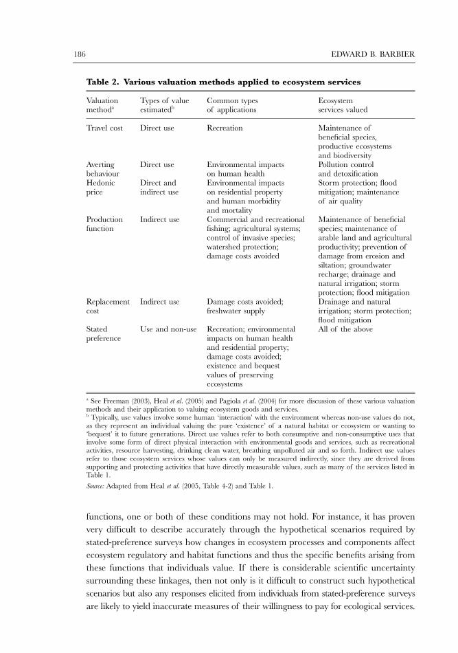
3.1. Methods of valuing ecosystem services
Table 2 indicates various methods that can be used for valuing ecological services.
2
However, some approaches are limited to specific benefits. For example, the travelcost method is used principally for environmental values that enhance individuals’enjoyment of recreation and tourism, averting behaviour models are best applied tothe health effects arising from pollution, and hedonic wage and property models areused primarily for assessing work-related hazards and environmental impacts onproperty values, respectively.
In contrast, stated preference methods, which include contingent valuation methods,conjoint analysis and choice experiments, have the potential to be used widely invaluing ecosystem goods and services. These valuation methods involve surveyingindividuals who benefit from an ecological service or range of services, and analysingthe responses to measure individuals’ willingness to pay for the service or services.
For example, choice experiments of wetland restoration in southern Swedenrevealed that individuals’ willingness to pay for the restoration increased if the resultenhanced overall biodiversity but decreased if the restored wetlands were used mainlyfor the introduction of Swedish crayfish for recreational fishing (Carlsson
et al.
, 2003).In some cases, stated preference methods are used to elicit ‘non-use values’, that is,the additional ‘existence’ and ‘bequest’ values that individuals attach to ensuring thata well-functioning system will be preserved for future generations to enjoy. A contin-gent valuation study of mangrove-dependent coastal communities in Micronesiademonstrated that the communities ‘place some value on the existence and ecosystemfunctions of mangroves over and above the value of mangroves’ marketable products’(Naylor and Drew, 1998, p. 488).
However, to implement a stated-preference study two key conditions are necessary:(1) the information must be available to describe the change in a natural ecosystemin terms of service that people care about, in order to place a value on those services;and (2) the change in the natural ecosystem must be explained in the survey instrumentin a manner that people will understand and not reject the valuation scenario (Heal
et al.
, 2005). For many of the services arising from ecological regulatory and habitat
2
It is beyond the scope of this paper to discuss all the valuation methods listed in Table 2. See Freeman (2003), Heal
et al.
(2005)and Pagiola
et al.
(2004) for more discussion of these various valuation methods and their application to valuing ecosystem goodsand services.
186 EDWARD B. BARBIER
functions, one or both of these conditions may not hold. For instance, it has provenvery difficult to describe accurately through the hypothetical scenarios required bystated-preference surveys how changes in ecosystem processes and components affectecosystem regulatory and habitat functions and thus the specific benefits arising fromthese functions that individuals value. If there is considerable scientific uncertaintysurrounding these linkages, then not only is it difficult to construct such hypotheticalscenarios but also any responses elicited from individuals from stated-preference surveysare likely to yield inaccurate measures of their willingness to pay for ecological services.
Table 2. Various valuation methods applied to ecosystem services
Valuation methoda
Types of value estimatedb
Common types of applications
Ecosystem services valued
Travel cost Direct use Recreation Maintenance of beneficial species, productive ecosystems and biodiversity
Averting behaviour
Direct use Environmental impacts on human health
Pollution control and detoxification
Hedonic price
Direct and indirect use
Environmental impacts on residential property and human morbidity and mortality
Storm protection; flood mitigation; maintenance of air quality
Productionfunction
Indirect use Commercial and recreational fishing; agricultural systems; control of invasive species; watershed protection; damage costs avoided
Maintenance of beneficial species; maintenance of arable land and agricultural productivity; prevention of damage from erosion and siltation; groundwater recharge; drainage and natural irrigation; storm protection; flood mitigation
Replacementcost
Indirect use Damage costs avoided; freshwater supply
Drainage and natural irrigation; storm protection; flood mitigation
Stated preference
Use and non-use Recreation; environmental impacts on human health and residential property; damage costs avoided; existence and bequest values of preserving ecosystems
All of the above
a See Freeman (2003), Heal et al. (2005) and Pagiola et al. (2004) for more discussion of these various valuationmethods and their application to valuing ecosystem goods and services.b Typically, use values involve some human ‘interaction’ with the environment whereas non-use values do not,as they represent an individual valuing the pure ‘existence’ of a natural habitat or ecosystem or wanting to‘bequest’ it to future generations. Direct use values refer to both consumptive and non-consumptive uses thatinvolve some form of direct physical interaction with environmental goods and services, such as recreationalactivities, resource harvesting, drinking clean water, breathing unpolluted air and so forth. Indirect use valuesrefer to those ecosystem services whose values can only be measured indirectly, since they are derived fromsupporting and protecting activities that have directly measurable values, such as many of the services listed inTable 1.
Source: Adapted from Heal et al. (2005, Table 4-2) and Table 1.
VALUING ECOSYSTEM SERVICES 187
In contrast to stated-preference methods, the advantage of PF approaches is thatthey depend on only the first condition, and not both conditions, holding. That is,for those regulatory and habitat functions where there is sufficient scientific knowl-edge of how these functions link to specific ecological services that support or protecteconomic activities, then it may be possible to employ the PF approach to value theseservices. However, PF methods have their own measurement issues and limitations.These are also discussed further in the rest of this section, and illustrated usingexamples of key ecological services from coastal and estuarine wetlands.
3.2. The production function approach
Many of the beneficial services derived from regulatory and habitat functions arecommonly classified by economists as indirect use values (Barbier, 1994). The benefitsattributed to these services arise through their support or protection of activities thathave directly measurable values (see Table 2). For example, coastal and estuarinewetlands, such as tropical mangroves and temperate marshlands, act as ‘naturalbarriers’ by preventing or mitigating storms and floods that could affect property andland values, agriculture, fishing and drinking supplies, as well as cause sickness anddeath. Similarly, coastal and estuarine wetlands may also provide a nursery andbreeding habitat that supports the productivity of near-shore fisheries, which in turnmay be valued for their commercial or recreational catch.
Because the benefits of these ecosystem services appear to enhance the productivityof economic activities, or protect them from possible damages, one possible methodof measuring the aggregate willingness to pay for such services is to estimate theirvalue as if they were a factor input in these productive activities. This is the essenceof the PF valuation approaches, also called ‘valuing the environment as input’(Barbier, 1994 and 2000; Freeman, 2003, ch. 9).
3
The basic modelling approach underlying PF methods is similar to determiningthe additional value of a change in the supply of any factor input. If changes in theregulatory and habitat functions of ecosystems affect the marketed productionactivities of an economy, then the effects of these changes will be transmitted toindividuals through the price system via changes in the costs and prices of final goodsand services. This means that any resulting ‘improvements in the resource base orenvironmental quality’ as a result of enhanced ecosystem services, ‘lower costs andprices and increase the quantities of marketed goods, leading to increases in consumers’and perhaps producers’ surpluses’ (Freeman, 2003, p. 259). The sum of consumerand producer surpluses in turn provides a measure of the willingness to pay for theimproved ecosystem services.
3
The concept of ‘valuing’ the environment as input is not new. Dose-response and change-in-productivity models, which havebeen used for some time, can be considered special cases of the PF approach in which the production responses to environmen-tal quality changes are greatly simplified (Freeman, 1982).
188 EDWARD B. BARBIER
An adaptation of the PF methodology is required in the case where ecologicalregulatory and habitat functions have a protective value, such as the storm protectionand flood mitigation services provided by coastal wetlands. In such cases, the envi-ronment may be thought of producing a non-marketed service, such as ‘protection’of economic activity, property and even human lives, which benefits individualsthrough limiting damages. Applying PF approaches requires modelling the ‘produc-tion’ of this protection service and estimating its value as an environmental input interms of the expected damages avoided.
Although this paper focuses mainly on applications of the PF approach to coastalwetland ecosystems, as Table 2 indicates PF approaches are being increasinglyemployed for a diverse range of environmental quality impacts and ecosystem ser-vices. Some examples include maintenance of biodiversity and carbon sequestration intropical forests (Boscolo and Vincent, 2003); nutrient reduction in the Baltic Sea(Gren
et al.
, 1997); pollination service of tropical forests for coffee production in CostaRica (Ricketts
et al.
, 2004); tropical watershed protection services (Kaiser andRoumasset, 2002); groundwater recharge supporting irrigation farming in Nigeria(Acharya and Barbier, 2000); coral reef habitat support of marine fisheries in Kenya(Rodwell
et al.
, 2002); marine reserves acting to enhance the ‘insurance value’ ofprotecting commercial fish species in Sicily (Mardle
et al.
, 2004) and in the northeastcod fishery (Sumaila, 2002); and nutrient enrichment in the Black Sea affecting thebalance between invasive and beneficial species (Knowler
et al.
, 2001).
3.3. Measurement issues for modelling habitat-fishery linkages
Applying PF methods to valuing ecosystem services has its own demands in terms ofecological and economic data. To highlight these additional measurement issues, thissection draws on the example of valuing coastal wetlands as a nursery and breedinghabitat for commercial near-shore fisheries.
First, application of the PF approach requires properly specifying the habitat-fishery PF model that links the physical effects of the change in this service to changesin market prices and quantities and ultimately to consumer and producer surpluses.As with many ecological services, it is difficult to measure directly changes in thehabitat and nursery function of coastal wetlands. Instead, the standard approachadopted in coastal habitat-fishery PF models is to allow the wetland area to serve asa proxy for the productivity contribution of the nursery and habitat function (seeBarbier, 2000 for further discussion). It is then relatively straightforward to estimatethe impacts of the change in the coastal wetland area input on fishery catch, in termsof the marginal costs of fishery harvests and thus changes in consumer and producersurpluses.
Second, market conditions and regulatory policies for the marketed output willinfluence the values imputed to the environmental input (Freeman, 1991). Forinstance, the offshore fishery supported by coastal wetlands may be subject to open
VALUING ECOSYSTEM SERVICES 189
access. Under these conditions, profits in the fishery would be dissipated, andequilibrium prices would be equated to average and not marginal costs. As aconsequence, there is no producer surplus, and the welfare impact of a change inwetland habitat is measured by the resulting change in consumer surplus only.
Third, if the ecological service supports a harvested natural resource system, suchas a fishery, forestry or a wildlife population, then it may be necessary to model howchanges in the stock or biological population may affect the future flow of benefits.If the natural resource stock effects are not considered significant, then the environ-mental changes can be modelled as impacting only current harvest, prices andconsumer and producer surpluses. If the stock effects are significant, then a changein an ecological service will impact not only current but also future harvest andmarket outcomes. In the PF valuation literature, the first approach is referred to as a‘static model’ of environmental change on a natural resource production system,whereas the second approach is referred to as a ‘dynamic model’ because it takes intoaccount the intertemporal stock effects of the environmental change (Barbier, 2000;Freeman, 2003, ch. 9).
Finally, most natural ecosystems provide more than one beneficial service, and itmay be important to model any trade-offs among these services as an ecosystem isaltered or disturbed. Integrated economic-ecological modelling could capture morefully the ecosystem functioning and dynamics underlying the provision of key services,and can be used to value multiple services arising from natural ecosystems. Forinstance, integrated modelling of an entire wetland-coral reef-sea grass system couldmeasure simultaneously the benefits of both the habitat-fishery linkage and the stormprotection service provided by the system. Examples of such multi-service ecosystemmodelling include analysis of salmon habitat restoration (Wu
et al.
, 2003); eutrophi-cation of small shallow lakes (Carpenter
et al.
, 1999); changes in species diversity ina marine ecosystem (Finnoff and Tschirhart, 2003); and introduction of exotic troutspecies (Settle and Shogren, 2002).
To illustrate the first three of the above issues, I next explore two ways of measur-ing the welfare effects of an environmental change on a productive natural resourcesystem with the example of the coastal habitat-fishery linkage. I will return to theissue of integrated ecological-economic modelling of multiple ecological services inSection 5.
3.3.1. Habitat-fishery linkages: static approaches.
This section illustrates theuse of a static model to value how a change in coastal wetland habitat area affectsthe market for commercially harvested fish. Many initial PF methods to value habitat-fishery linkages have relied on this static approach. For example, using data from theLynne
et al.
(1981), Ellis and Fisher (1987) constructed such a model to value thesupport by Florida marshlands for Gulf Coast crab fisheries in terms of the resultingchanges in consumer and producer surpluses from the marketed catch. Freeman(1991) then extended Ellis and Fisher’s approach to show how the values imputed to

190 EDWARD B. BARBIER
the wetlands in the static model is influenced by whether or not the fishery isopen access or optimally managed. Sathirathai and Barbier (2001) also used a staticmodel of habitat-fishery linkages to value the role of mangroves in Thailand insupporting near-shore fisheries under both open access and optimally managedconditions.
As most near-shore fisheries are not optimally managed but open access, the followingillustration of the static model of habitat-fishery linkages assumes that the fishery isopen access. Any profits in the fishery will attract new entrants until all the profitsdisappear, and in equilibrium, the welfare change in coastal wetland is in terms of itsimpact on consumer surplus only.
As noted above, the general PF approach treats an ecological service, such ascoastal wetland habitat, as an ‘input’ into the economic activity, and like any otherinput, its value can be equated with its impact on the productivity of any marketedoutput. More formally, if
h
is the marketed harvest of the fishery, then its productionfunction can be denoted as:
h
=
h
(
E
i
. . .
E
k
,
S
) (1)
The area of coastal wetlands,
S
, may therefore have a direct influence on the marketedfish catch,
h
, which is independent from the standard inputs of a commercial fishery,
E
i
. . . E
k
.A standard assumption in most static habitat-fishery models is that the production
function (1) takes the Cobb–Douglas form,
h
=
AE
a
S
b
, where
E
is some aggregatemeasure of total effort in the off-shore fishery and
S
is coastal wetland habitat area.It follows that the optimal cost function of a cost-minimizing fishery is:
C
* =
C
(
h
,
w
,
S
) =
wA
−
1/
a
h
1/
a
S
−
b
/
a
(2)
where
w
is the unit cost of effort. Assuming an iso-elastic market demand function,
P
=
p
(
h
) =
kh
η
, η = 1/ε < 0 , then the market equilibrium for catch of the open accessfishery occurs where the total revenues of the fishery just equals cost, or price equalsaverage cost, i.e. P = C */h, which in this model becomes:
khη = wA−1/ah1−a/aS −b/a (3)
which can be rearranged to yield the equilibrium level of fish harvest:
(4)
It follows from (4) that the marginal impact of a change in wetland habitat is:
(5)
The change in consumer surplus, CS, resulting from a change in equilibriumharvest levels (from h0 to h1) is:
hwk
A S aa
b , ( ) /
/ /=
= + −− −
ββ β β η1 1 1
dhdS
b wk
A Sa
b /
/ ( )/= −
− − +
β
ββ β β1
VALUING ECOSYSTEM SERVICES 191
(6)
By utilizing (5) and (6) it is possible to estimate the new equilibrium harvest andprice levels and thus the corresponding changes in consumer surplus associated witha change in coastal wetland area, for a given demand elasticity, γ.
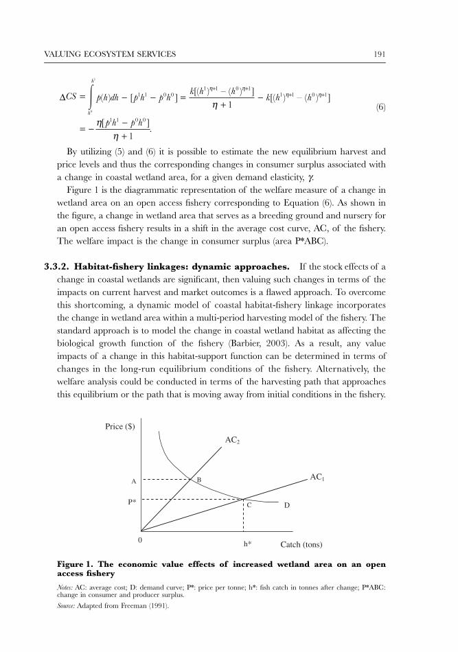
Figure 1 is the diagrammatic representation of the welfare measure of a change inwetland area on an open access fishery corresponding to Equation (6). As shown inthe figure, a change in wetland area that serves as a breeding ground and nursery foran open access fishery results in a shift in the average cost curve, AC, of the fishery.The welfare impact is the change in consumer surplus (area P*ABC).
3.3.2. Habitat-fishery linkages: dynamic approaches. If the stock effects of achange in coastal wetlands are significant, then valuing such changes in terms of theimpacts on current harvest and market outcomes is a flawed approach. To overcomethis shortcoming, a dynamic model of coastal habitat-fishery linkage incorporatesthe change in wetland area within a multi-period harvesting model of the fishery. Thestandard approach is to model the change in coastal wetland habitat as affecting thebiological growth function of the fishery (Barbier, 2003). As a result, any valueimpacts of a change in this habitat-support function can be determined in terms ofchanges in the long-run equilibrium conditions of the fishery. Alternatively, thewelfare analysis could be conducted in terms of the harvesting path that approachesthis equilibrium or the path that is moving away from initial conditions in the fishery.
∆CS p h dh p h p hk h h
k h h
p h p hh
h
( ) [ ] [( ) – ( ) ]
[( ) – ( ) ]
[ ]
.
= − − =+
−
= −−+
+ ++ +�
0
1
1 1 0 01 1 0 1
1 1 0 1
1 1 0 0
1
1
η ηη η
η
ηη
Figure 1. The economic value effects of increased wetland area on an openaccess fishery
Notes: AC: average cost; D: demand curve; P*: price per tonne; h*: fish catch in tonnes after change; P*ABC:change in consumer and producer surplus.
Source: Adapted from Freeman (1991).
192 EDWARD B. BARBIER
Most attempts to value habitat-fishery linkages via a dynamic model that incorporatesstock effects have assumed that the fishery affected by the habitat change is in a long-runequilibrium. Such a model has been applied, for example, in case studies of valuinghabitat fishery linkages in Mexico (Barbier and Strand, 1998), Thailand (Barbier etal., 2002; Barbier, 2003) and the United States (Swallow, 1994). Similar ‘equilibrium’dynamic approaches have been used to model other coastal environmental changes,including the impacts of water quality on fisheries in the Chesapeake Bay (Kahn andKemp, 1985; McConnell and Strand, 1989) and the effects of mangrove deforestationand shrimp larvae availability on aquaculture in Ecuador (Parks and Bonifaz, 1997).
However, valuing the change in coastal wetland habitat in terms of its impact onthe long-run equilibrium of the fishery raises additional methodological issues. First,the assumption of prevailing steady state conditions is strong, and may not be arealistic representation of harvesting and biological growth conditions in the near-shore fisheries. Second, such an approach ignores both the convergence of stock andharvest to the steady state and the short-run dynamics associated with the impacts ofthe change in coastal habitat on the long-run equilibrium. The usual assumption isthat this change will lead to an instantaneous adjustment of the system to a newsteady state, but this in turn requires local stability conditions that may not be supportedby the parameters of the model.
There are examples of pure fisheries models that assume that the dynamic systemis not in equilibrium but is either on the approach to a steady state or is moving awayfrom initial fixed conditions. The latter approach has proven particularly useful in thecase of open access or regulated access fisheries (Bjørndal and Conrad, 1987; Homans andWilen, 1997). The following model shows how this approach can be adopted here tothe case of valuing a change in wetland habitat in terms of the dynamic path of anopen access fishery.
Defining Xt as the stock of fish measured in biomass units, any net change ingrowth of this stock over time can be represented as:
(7)
Thus, net expansion in the fish stock occurs as a result of biological growth in thecurrent period, F (Xt−1, St−1), net of any harvesting, h(Xt−1, Et−1), which is a function ofthe stock as well as fishing effort, Et−1. The influence of the wetland habitat area, St−1,as a breeding ground and nursery habitat on growth of the fish stock is assumed tobe positive, ∂F/∂St−1 > 0, as an increase in wetland area will mean more carryingcapacity for the fishery and thus greater biological growth.
As before, it is assumed that the near-shore fishery is open access. The standardassumption for an open access fishery is that effort next period will adjust in responseto the real profits made in the past period (Clark, 1976; Bjørndal and Conrad, 1987).Letting p(h) represent landed fish price per unit harvested, w the unit cost of effortand φ > 0 the adjustment coefficient, then the fishing effort adjustment equation is:
X X F X S h X EF
XF
St t t t t tt t
( , ) ( , ), , .− = − > >− − − − −− −
1 1 1 1 1
2
12
1
0 0∂∂
∂∂
VALUING ECOSYSTEM SERVICES 193
(8)
Assume a conventional bioeconomic fishery model with biological growth character-ized by a logistic function, F (Xt−1, St−1) = rXt−1[1 − Xt−1/K (St−1)], and harvesting by aSchaefer production process, ht = qXtEt, where q is a ‘catchability’ coefficient, r is theintrinsic growth rate and K (St) = α ln St, is the impact of coastal wetland area oncarrying capacity, K, of the fishery. The market demand function for harvested fish isagain assumed to be iso-elastic, i.e. p(h) = khη, η = 1/ε < 0. Substituting theseexpressions into (7) and (8) yields:
(9)
(10)
Both Xt and Et are predetermined, and so (9) and (10) can be estimated independently(see Homans and Wilen, 1997). Following Schnute (1977), define the catch per uniteffort as ct = ht/Et = qXt. If Xt is predetermined so is ct. Substituting the expressionfor catch per unit effort in (9) produces:
(11)
Thus Equations (10) and (11) can also be estimated independently to determine thebiological and economic parameters of the model. For given initial effort, harvest andwetland data, both the effort and stock paths of the fishery can be determined forsubsequent periods, and the consumer plus producer surplus can be estimated foreach period. Alternative effort and stock paths can then be determined as wetlandarea changes in each period, and thus the resulting changes in consumer plus pro-ducer surplus in each period are the corresponding estimates of the welfare impactsof the coastal habitat change.4
3.4. Replacement cost and cost of treatment
In circumstances where an ecological service is unique to a specific ecosystem and isdifficult to value, then economists have sometimes resorted to using the cost of replac-ing the service as a valuation approach.5 This method is usually invoked because ofthe lack of data for many services arising from natural ecosystems.
For example, the presence of a wetland may reduce the cost of municipal watertreatment because the wetland system filters and removes pollutants. It is therefore
4 As along its dynamic path the open access fishery is not in equilibrium, producer surpluses, or losses, are relevant for thewelfare estimate of a change in coastal wetland habitat.5 Such an approach to approximating the benefits of a service by the cost of providing an alternative is not used exclusively inenvironmental valuation. For example, in the health economics literature this approach is referred to as ‘cost of illness’ (Dickie, 2003).This involves adding up the costs of treating a patient for an illness as the measure of the benefit to the patient of staying disease-free.
E E p h h X E wEp hht t t t t t
t
t
[ ( ) ( , ) ], ( )
.− = − <− − − − −−
−1 1 1 1 1
1
1
0φ ∂∂
X rXX
Sh Xt t
t
tt t
ln = −
− +−
−
−− −1
1
11 11
α
E R w E R kht t t t t ( ) , .= + − =− − − −+φ φ η
1 1 1 111
c cc
rr
qcS
qEt t
t
t
tt
ln .
−= − −−
−
−
−−
1
1
1
11α
194 EDWARD B. BARBIER
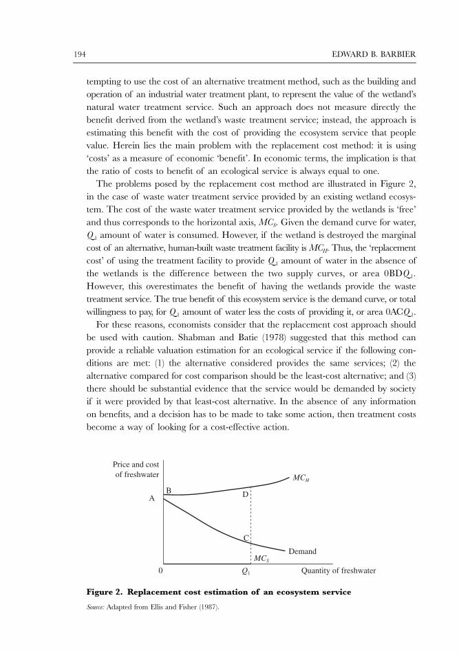
tempting to use the cost of an alternative treatment method, such as the building andoperation of an industrial water treatment plant, to represent the value of the wetland’snatural water treatment service. Such an approach does not measure directly thebenefit derived from the wetland’s waste treatment service; instead, the approach isestimating this benefit with the cost of providing the ecosystem service that peoplevalue. Herein lies the main problem with the replacement cost method: it is using‘costs’ as a measure of economic ‘benefit’. In economic terms, the implication is thatthe ratio of costs to benefit of an ecological service is always equal to one.
The problems posed by the replacement cost method are illustrated in Figure 2,in the case of waste water treatment service provided by an existing wetland ecosys-tem. The cost of the waste water treatment service provided by the wetlands is ‘free’and thus corresponds to the horizontal axis, MCS. Given the demand curve for water,Q 1 amount of water is consumed. However, if the wetland is destroyed the marginalcost of an alternative, human-built waste treatment facility is MCH. Thus, the ‘replacementcost’ of using the treatment facility to provide Q 1 amount of water in the absence ofthe wetlands is the difference between the two supply curves, or area 0BDQ 1.However, this overestimates the benefit of having the wetlands provide the wastetreatment service. The true benefit of this ecosystem service is the demand curve, or totalwillingness to pay, for Q 1 amount of water less the costs of providing it, or area 0ACQ 1.
For these reasons, economists consider that the replacement cost approach shouldbe used with caution. Shabman and Batie (1978) suggested that this method canprovide a reliable valuation estimation for an ecological service if the following con-ditions are met: (1) the alternative considered provides the same services; (2) thealternative compared for cost comparison should be the least-cost alternative; and (3)there should be substantial evidence that the service would be demanded by societyif it were provided by that least-cost alternative. In the absence of any informationon benefits, and a decision has to be made to take some action, then treatment costsbecome a way of looking for a cost-effective action.
Figure 2. Replacement cost estimation of an ecosystem service
Source: Adapted from Ellis and Fisher (1987).
VALUING ECOSYSTEM SERVICES 195
One of the best-known examples of a policy decision based on using the ‘replace-ment cost’ method to assess the value of an ecosystem service is the provision of cleandrinking water by the Catskills Mountains for New York City (Heal et al., 2005). In1996, New York City faced a choice: either it could build water filtration systems toclean its water supply or the city could restore and protect the Catskill watersheds toensure high-quality drinking water. Because estimates indicated that building andoperating the filtration system would cost $6–8 billion whereas protecting and restoringthe watersheds would cost $1–1.5 billion, New York chose to protect the Catskills. Inthis case, it was sufficient for the policy decision simply to demonstrate the cost-effectiveness of restoring and protecting the ecological integrity of the Catskills watershedscompared to the alternative of the human-constructed water filtration system. Thus,clearly this is an example where the criteria established by Shabman and Batie (1978)apply.
The main reason why economists have resorted to replacement cost approaches tovaluing an ecosystem service, however, is that there is often a lack of data on thelinkage between the initial ecological function, the processes and components ofecosystems that facilitate this function, and the eventual ecological service thatbenefits humans. The lack of such data makes it extremely difficult to constructreliable hypothetical scenarios through stated preference surveys and similar methodsto elicit accurate responses from individuals about their willingness to pay forecological services. As an illustration, in the Catskills case study, a stated preferencesurvey may have elicited an estimate of the total willingness-to-pay by New York Cityresidents for the amount of freshwater provided – for example, the total demand forfreshwater Q 1 in Figure 2 – but it would have been very difficult to obtain a measureof the willingness-to-pay to avoid losses in the water treatment service that occurthrough changes in the land use in Catskills watershed that affect the free provision ofthis ecological service.
Similarly, as pointed out by Chong (2005), it is very difficult to use stated preferencemethods in tropical developing areas to assess the benefits to local communitiesof the storm protection service of mangrove systems. Although there is sufficientscientific evidence suggesting that such a service occurs, there is a lack of ecologicaldata on how loss of mangroves in specific locations will affect their ability toprovide storm protection to neighbouring communities. To date, the few studiesthat have attempted to value the storm prevention and flood mitigation servicesof the ‘natural’ storm barrier function of mangrove systems have employed thereplacement cost method by simply estimating the costs of replacing mangroveswith constructed barriers that perform the same services (Chong, 2005). Unfortu-nately, such estimates not only make the classic error of estimating a ‘benefit’ bya ‘cost’ but also may yield unrealistically high estimates, given that removing all themangroves and replacing them with constructed barriers is unlikely to be the least-cost alternative to providing storm prevention and flood mitigation services in coastalareas.
196 EDWARD B. BARBIER
3.5. Expected damage function approach
For some ecological services, an alternative to employing replacement cost methodsmight be the expected damage function (EDF) approach.6
The EDF approach, which is a special category of ‘valuing’ the environment as‘input’, is nominally straightforward; it assumes that the value of an asset that yieldsa benefit in terms of reducing the probability and severity of some economic damageis measured by the reduction in the expected damage. The essential step to imple-menting this approach, which is to estimate how changes in the asset affect theprobability of the damaging event occurring, has been used routinely in risk analysisand health economics, for example, as in the case of airline safety performance (Rose,1990); highway fatalities (Michener and Tighe, 1992); drug safety (Olson, 2004); andstudies of the incidence of diseases and accident rates (Cameron and Trivedi, 1998;Winkelmann, 2003). Here we show that the EDF approach can also be applied,under certain circumstances, to value ecological services that also reduce the prob-ability and severity of economic damages.
Recall that one of the special features of many regulatory and habitat services ofecosystems is that they may protect nearby economic activities, property and evenhuman lives from possible damages. As indicated in Table 1, such services includestorm protection, flood mitigation, prevention of erosion and siltation, pollution con-trol and maintenance of beneficial species. The EDF approach essentially ‘values’these services through estimating how they mitigate damage costs.
The following example illustrates how the expected damage function (EDF) methodologycan be applied to value the storm protection service provided by a coastal wetland,such as a marshland or mangrove ecosystem. The starting point is the standard‘compensating surplus’ approach to valuing a quantity or quality change in a non-market environmental good or service (Freeman, 2003).
Assume that in a coastal region the local community owns all economic activityand property, which may be threatened by damage from periodic natural stormevents. Assume also that the preferences of all households in the community aresufficiently identical so that it can be represented by a single household. Letm(px, z, u0) be the expenditure function of the representative household, that is, theminimum expenditure required by the household to reach utility level, u0, given thevector of prices, px, for all market-purchased commodities consumed by the household,the expected number or incidence of storm events, z0.
Suppose the expected incidence of storms rises from z0 to z1. The resultingexpected damages to the property and economic livelihood of the household, E[D(z)],translates into an exact measure of welfare loss through changes in the minimumexpenditure function:
6 The expected damage function approach predates many of the PF methods discussed so far, and has been used extensively toestimate the risk of health impacts from pollution (Freeman, 1982, chs. 5 and 9).
VALUING ECOSYSTEM SERVICES 197
E[D(z)] = m(px, z1, u0) − m(px, z0, u0) = c(z) (12)
where c(z) is the compensating surplus. It is the minimum income compensation thatthe household requires to maintain it at the utility level u0, despite the expectedincrease in damaging storm events. Alternatively, c(z) can be viewed as the minimumincome that the household needs to avoid the increase in expected storm damages.
However, the presence of coastal wetlands could mitigate the expected incidenceof damaging storm events. Because of this storm protection service, the area of coastalwetlands, S, may have a direct effect on reducing the ‘production’ of natural disasters,in terms of their ability to inflict damages locally. Thus the ‘production function’ forthe incidence of potentially damaging natural disasters can be represented as:
z = z(S ), z′ < 0, z″ > 0. (13)
It follows from (12) and (13) that ∂c(z)/∂S = ∂E[D(z)]/∂S < 0. An increase in wetlandarea reduces expected storm damages and therefore also reduces the minimumincome compensation needed to maintain the household at its original utility level.Alternatively, a loss in wetland area would increase expected storm damages andraises the minimum compensation required by the household to maintain its welfare.Thus, we can define the marginal willingness to pay, W(S ), for the protection servicesof the wetland in terms of the marginal impact of a change in wetland area onexpected storm damages:
(14)
The ‘marginal valuation function’, W(S ), is analogous to the Hicksian compensateddemand function for marketed goods. The minus sign on the right-hand sign of (14)allows this ‘demand’ function to be represented in the usual quadrant, and it has thenormal downward-sloping property (see Figure 3). Although an increase in S reducesz and thus enables the household to avoid expected damages from storms, the addi-tional value of this storm protection service to the household will fall as wetland areaincreases in size. This relationship should hold across all households in the coastalcommunity. Consequently, as indicated in Figure 3, the marginal willingness to payby the community for more storm protection declines with S.
The value of a non-marginal change in wetland area, from S0 to S1, can bemeasured as:
(15)
If there is an increase in wetland area, then the value of this change is the totalamount of expected damage costs avoided. If there is a reduction in wetland area, asshown in Figure 3, then the welfare loss is the total expected damages resulting fromthe increased incidence of storm events. As indicated in (15), in both instances the
W SE D z S
SE
Dz
z W( ) [ ( ( ))]
, .= − = − ′
′ <
∂∂
∂∂
0
− = = ( ) [ ( ( ))] ( ).�S
S
W S dS E D z S c S
0
1
198 EDWARD B. BARBIER
valuation would be a compensation surplus measure of a change in the area ofwetlands and the storm protection service that they provide.
As indicated in (14), an estimate of the marginal impact of a change in wetlandarea on expected storm damages has two components: the influence of wetland areaon the expected incidence of economically damaging natural disaster events, z′, andsome measure of the additional economic damage incurred per event. Thus the right-hand expression in (14) can be estimated, provided that there are sufficient data onpast storm events, and preferably across different coastal areas, and some estimate ofthe economic damages inflicted by each event. The most important step in theanalysis is the first one, using the data on the incidence of past natural disasters andchanges in wetland area in coastal areas to estimate z(S ). One way this analysis canbe done is through employing count data models.
Count data models explain the number of times a particular event occurs over agiven period. In economics, count data models have been used to explain a varietyof phenomenon, such as explaining successful patents derived from firm R&D expen-ditures, accident rates, disease incidence, crime rates and recreational visits (Cameronand Trivedi, 1998; Greene, 2003, ch. 21; Winkelmann, 2003). Count data modelscould be used to estimate whether a change in the area of coastal wetlands, S, reducesthe expected incidence of economically damaging storm events. The basic methodologyfor such an application of count data models is described further in the appendix.
However, applying the EDF method to estimating the storm protection value ofcoastal wetlands raises two additional measurement issues.
First, as the 2004 Asian tsunami and recent hurricanes in the United States havedemonstrated, the risks to vulnerable populations living in coastal areas from theeconomic damages of storm events can be very large. This suggests that coastalpopulations will display a degree of risk aversion to such events, in the sense that theywould like to see the least possible variance in expected storm damages. Applyingstandard techniques, such as the capital-asset pricing model, this implies in turn that
Figure 3. Expected damage costs from a loss of wetland area
VALUING ECOSYSTEM SERVICES 199
there should be a ‘risk premium’ attached to the storm protection value of coastalwetlands that reduces the variance in expected economic damages from storm events(Hirshleifer and Riley, 1992).
Second, estimating how coastal wetlands affect the expected number of economicdamaging events from the count data model and then multiplying the effect by theaverage economic damages across events could be misleading under some extremecircumstances. For instance, suppose a loss in wetland area is associated with a situ-ation in which there is a change in the incidence of storms from one devastatingstorm to two relatively minor storms per year. The count data model would then beinterpreted as not providing evidence against the null that the change in the wetlandarea increases expected storm damages. Clearly, there needs to be a robustness checkon the count data model to ensure that such situations do not dominate the applica-tion of the EDF approach.
4. CASE STUDY OF MANGROVE ECOSYSTEMS IN THAILAND
This section illustrates the application of the PF approach and the EDF approach tovaluation of ecological services with a case study of mangrove ecosystems in Thailand.The two services of interest are the provision of a breeding and nursery habitat forfisheries and the storm protection service of mangroves.
Both the dynamic and static PF approaches are used to estimate the value of themangrove-fishery habitat service. The EDF approach to estimating the storm protectionservice of mangroves is contrasted with the replacement cost method.
4.1. Case study background
Many mangrove ecosystems, especially those in Asia, are threatened by rapiddeforestation. At least 35% of global mangrove area has been lost in the past twodecades; in Asia, 36% of mangrove area has been deforested, at the rate of 1.52%per year (Valiela et al., 2001). Although many factors are behind global mangrovedeforestation, a major cause is aquaculture expansion in coastal areas, especially theestablishment of shrimp farms (Barbier and Cox, 2003). Aquaculture accounts for52% of mangrove loss globally, with shrimp farming alone accounting for 38% ofmangrove deforestation; in Asia, aquaculture contributes 58% to mangrove loss withshrimp farming accounting for 41% of total deforestation (Valiela et al., 2001).
Mangrove deforestation has been particularly prevalent in Thailand. Some estimatessuggest that over 1961–96 Thailand lost around 2050 km2 of mangrove forests, orabout 56% of the original area, mainly due to shrimp aquaculture and other coastaldevelopments (Charuppat and Charuppat, 1997). Since 1975, 50–65% of Thailand’smangroves have been converted to shrimp farms (Aksornkoae and Tokrisna, 2004).
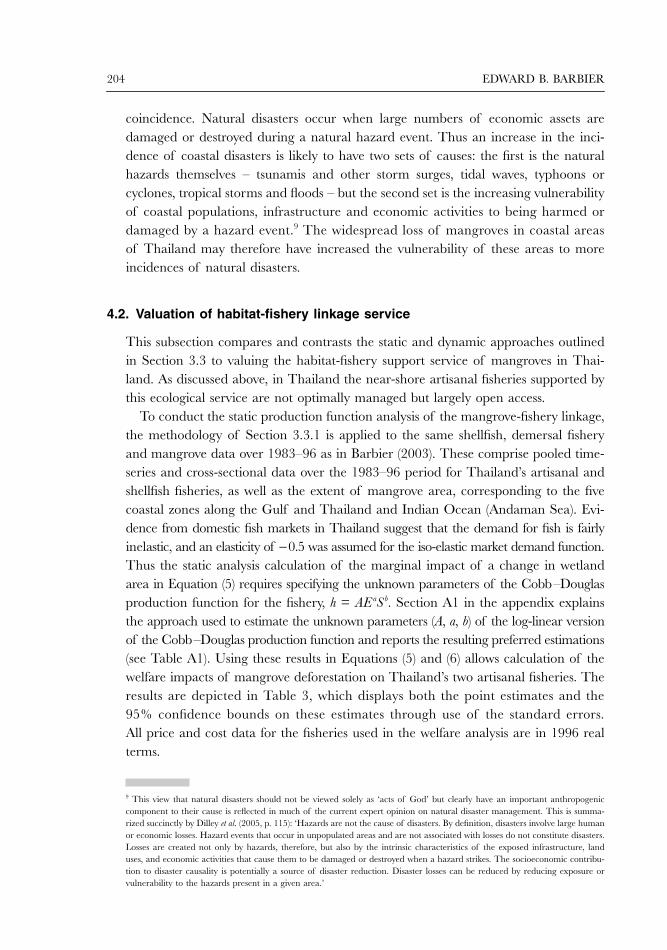
Figure 4 shows two long-run trend estimates of mangrove area in Thailand. In1961, there were approximately 3700 km2 of mangroves, which declined steadily to
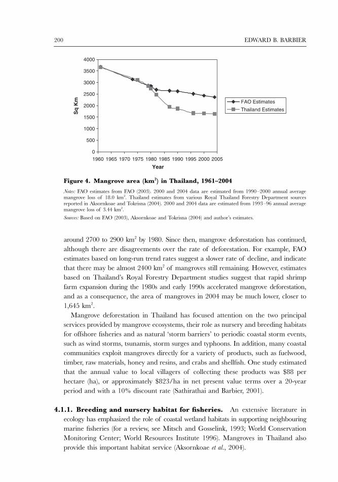
200 EDWARD B. BARBIER
around 2700 to 2900 km2 by 1980. Since then, mangrove deforestation has continued,although there are disagreements over the rate of deforestation. For example, FAOestimates based on long-run trend rates suggest a slower rate of decline, and indicatethat there may be almost 2400 km2 of mangroves still remaining. However, estimatesbased on Thailand’s Royal Forestry Department studies suggest that rapid shrimpfarm expansion during the 1980s and early 1990s accelerated mangrove deforestation,and as a consequence, the area of mangroves in 2004 may be much lower, closer to1,645 km2.
Mangrove deforestation in Thailand has focused attention on the two principalservices provided by mangrove ecosystems, their role as nursery and breeding habitatsfor offshore fisheries and as natural ‘storm barriers’ to periodic coastal storm events,such as wind storms, tsunamis, storm surges and typhoons. In addition, many coastalcommunities exploit mangroves directly for a variety of products, such as fuelwood,timber, raw materials, honey and resins, and crabs and shellfish. One study estimatedthat the annual value to local villagers of collecting these products was $88 perhectare (ha), or approximately $823/ha in net present value terms over a 20-yearperiod and with a 10% discount rate (Sathirathai and Barbier, 2001).
4.1.1. Breeding and nursery habitat for fisheries. An extensive literature inecology has emphasized the role of coastal wetland habitats in supporting neighbouringmarine fisheries (for a review, see Mitsch and Gosselink, 1993; World ConservationMonitoring Center; World Resources Institute 1996). Mangroves in Thailand alsoprovide this important habitat service (Aksornkoae et al., 2004).
Figure 4. Mangrove area (km2) in Thailand, 1961–2004
Notes: FAO estimates from FAO (2003). 2000 and 2004 data are estimated from 1990–2000 annual averagemangrove loss of 18.0 km2. Thailand estimates from various Royal Thailand Forestry Department sourcesreported in Aksornkoae and Tokrisna (2004). 2000 and 2004 data are estimated from 1993–96 annual averagemangrove loss of 3.44 km2.
Sources: Based on FAO (2003), Aksornkoae and Tokrisna (2004) and author’s estimates.
VALUING ECOSYSTEM SERVICES 201
Thailand’s coastline is vast, stretching for 2815 km, of which 1878 km is on theGulf of Thailand and 937 km on the Andaman Sea (Indian Ocean) (Kaosa-ard andPednekar, 1998). Since 1972, the 3 km offshore coastal zone in southern Thailandhas been reserved for small-scale, artisanal marine fisheries. The Gulf of Thailand isdivided into four such major zones, and the Andaman Sea comprises a fifth zone.7
The mangroves along these coastal zones are thought to provide breeding groundsand nurseries in support of several species of demersal fish and shellfish (mainly craband shrimp) in Thailand’s coastal waters.8 The artisanal marine fisheries of the fivemajor coastal zones of Thailand depend largely on shellfish but also some demersalfish. For example, in 1994 shrimp, crab, squid and cuttlefish alone accounted for 67%of all catch in the artisanal marine fisheries, and demersal fish accounted for 5.3%(Kaosa-ard and Pednekar, 1998).
The coastal artisanal fisheries of Thailand are characterized by classic open accessconditions (Kaosa-ard and Pedneker, 1998; Wattana, 1998). Since the 1970s, therehave been approximately 36 000–38 000 households engaged in small-scale fishingactivities. Although there are 2500 fishing communities scattered over the 24 coastalprovinces of Thailand, 90% of the artisanal fishing households are concentrated incommunities spread along the Southern Gulf of Thailand and Andaman Sea coasts.While the number of households engaged in small-scale fishing has remained fairlystable since 1985, the use of motorized boats has increased by more than 30%(Wattana, 1998). Gill nets still remain the most common form of fishing gear usedby artisanal fishers. Although a licence fee and permit are required for fishing incoastal waters, officials do not strictly enforce the law and users do not pay. Currently,there is no legislation for supporting community-based fishery management (Kaosa-ard and Pednekar, 1998).
4.1.2. Storm protection. The 26 December 2004 Indian Ocean tsunami disasterhas focused attention on the role of natural barriers, such as mangroves, in protectingvulnerable coastlines and populations in the region from such storm events (UNEP,2005; Wetlands International, 2005). Mangrove wetlands, which are found alongsheltered tropical and subtropical shores and estuaries, are particularly valuable inminimizing damage to property and loss of human life by acting as a barrier againsttropical storms, such as typhoons, cyclones, hurricanes and tsunamis (Chong, 2005;Massel et al., 1999; Mazda et al., 1997). Evidence from the 12 Indian Ocean countriesaffected by the tsunami disaster, including Thailand, suggests that those coastal areas
7 The four Gulf of Thailand zones consist of the following coastal provinces: Trat, Chantaburi and Rayong (Zone 1); ChonBuri, Chachoengsao, Samut Parkakan, Samut Sakhon, Samut Songkhram, Phetchaburi, Prachaup Khiri Khan (Zone 2);Chumphon, Surat Thani, Nakhon Si Thammarat (Zone 3); and Songkhla, Patthani, Narathiwart (Zone 4). The fifth zone onthe Indian Ocean (Andaman Sea) consists of the following coastal provinces: Ranong, Phangnga, Phuket, Krabi, Trang andSatun (Zone 5).8 Mangrove-dependent demersal fish include those belonging to the Clupeidae, Chanidae, Ariidae, Pltosidae, Mugilidae, Lujanidae andLatidae families. The shellfish include those belonging to the families of Panaeidae for shrimp and Grapsidae, Ocypodidae and Portnidaefor crab.
202 EDWARD B. BARBIER
that had dense and healthy mangrove forests suffered fewer losses and less damageto property than those areas in which mangroves had been degraded or converted toother land uses (Dahdouh-Guebas et al., 2005; Harakunarak and Aksornkoae, 2005;Kathiresan and Rajendran, 2005; UNEP, 2005; Wetlands International, 2005).
In Thailand, the Asian tsunami affected all six coastal provinces along the IndianOcean (Andaman Sea) coast: Krabi, Phang Nga, Phuket, Ranong, Satun and Trang.In Phang Nga, the most affected province, post-tsunami assessments suggest thatlarge mangrove forests in the north and south of the province significantly mitigatedthe impact of the Tsunami. They suffered damage on their seaside fringe, butreduced the tidal wave energy, providing protection to the inland population (UNEP,2005; Harakunarak and Aksornkoae, 2005). Similar results were reported for thoseshorelines in Ranong Province protected by dense and thriving mangrove forests. Incontrast, damages were relatively extensive along the Indian Ocean coast wheremangroves and other natural coastal barriers were removed or severely degraded(Harakunarak and Aksornkoae, 2005).
With the overwhelming evidence of the storm protection service provided by intactand healthy mangrove systems, since the tsunami disaster increased emphasis hasbeen placed on replanting degraded and deforested mangrove areas in Asia as ameans to bolstering coastal protection. For example, the Indonesian Minister forForestry has announced plans to reforest 600 000 hectares of depleted mangroveforest throughout the nation over the next 5 years. The governments of Sri Lankaand Thailand have also stated publicly intentions to rehabilitate and replant man-grove areas (UNEP, 2005; Harakunarak and Aksornkoae, 2005).
Although the Asian tsunami has called attention to the storm protection serviceprovided by mangroves, the benefits of this service extends to protection against manytypes of periodic coastal natural disaster events. As one post-tsunami assessmentnoted: ‘It is important to recognize that any compromising of mangrove “protectionfunction” is relevant to a wide variety of storm events, and not just tsunamis. Whereasthe Indian Ocean area counted “only” 63 tsunamis between 1750 and 2004, therewere more than three tropical cyclones per year in roughly the same area’ (Dahdouh-Guebas et al., 2005, pp. 445–6).
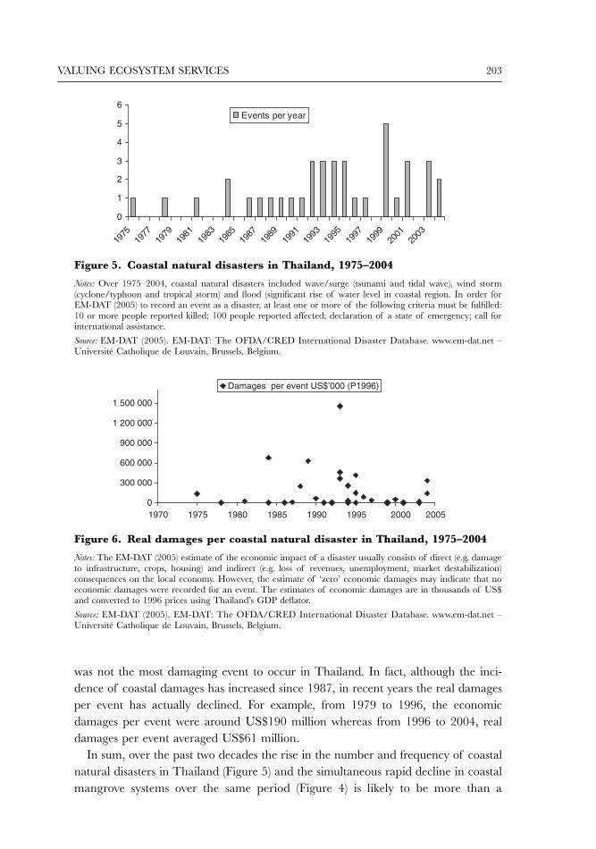
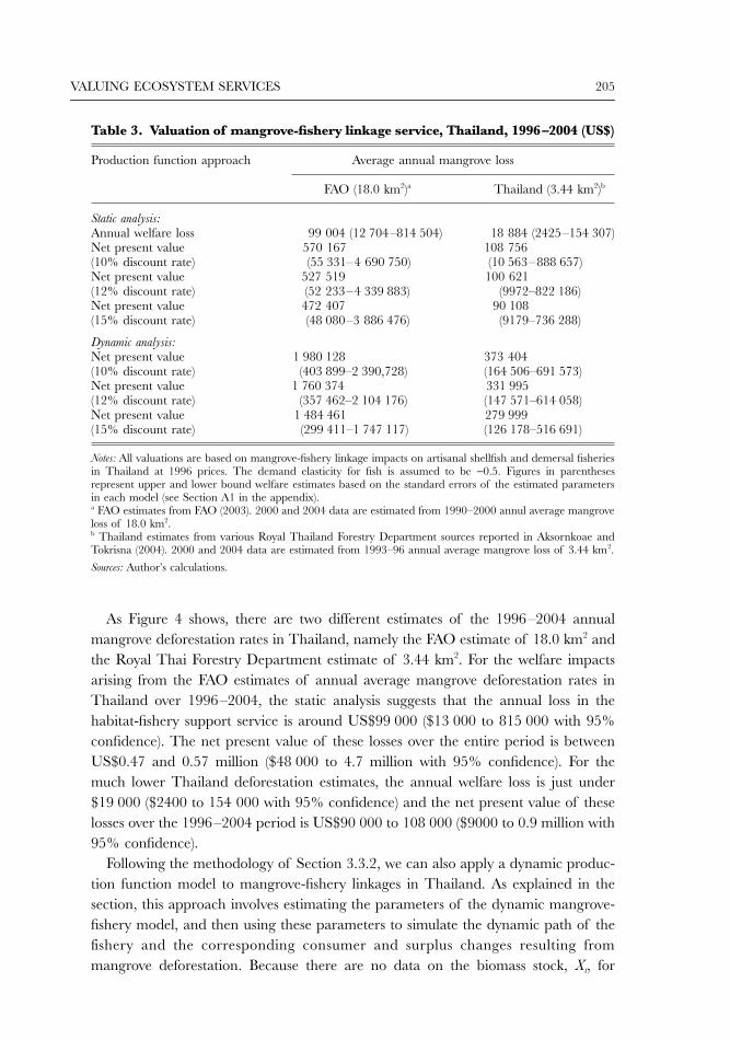
The EM-DAT International Disaster Database shows that the number of coastalnatural disasters in Thailand has increased in both the frequency of occurrence andin the number of events per year (see Figure 5). Over 1975–87, Thailand experiencedon average 0.54 coastal natural disasters per year, whereas between 1987–2004 theincidence increased to 1.83 disasters per year. Thus, a recent World Bank reportidentified the coastal and delta areas of Thailand as potentially high fatality (morethan 1000 deaths per event) and other damage ‘hotspots’ at risk from storm surgeevents (Dilley et al., 2005, pp. 101–3).
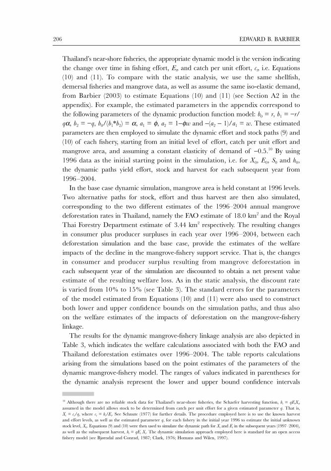
The EM-DAT database also calculates the economic damage incurred per event.Figure 6 plots the damages per coastal natural disaster in Thailand for 1975–2004.The 2004 Asian tsunami with estimated damages of US$240 million (1996 prices)
VALUING ECOSYSTEM SERVICES 203
was not the most damaging event to occur in Thailand. In fact, although the inci-dence of coastal damages has increased since 1987, in recent years the real damagesper event has actually declined. For example, from 1979 to 1996, the economicdamages per event were around US$190 million whereas from 1996 to 2004, realdamages per event averaged US$61 million.
In sum, over the past two decades the rise in the number and frequency of coastalnatural disasters in Thailand (Figure 5) and the simultaneous rapid decline in coastalmangrove systems over the same period (Figure 4) is likely to be more than a
Figure 5. Coastal natural disasters in Thailand, 1975–2004
Notes: Over 1975–2004, coastal natural disasters included wave/surge (tsunami and tidal wave), wind storm(cyclone/typhoon and tropical storm) and flood (significant rise of water level in coastal region. In order forEM-DAT (2005) to record an event as a disaster, at least one or more of the following criteria must be fulfilled:10 or more people reported killed; 100 people reported affected; declaration of a state of emergency; call forinternational assistance.
Source: EM-DAT (2005). EM-DAT: The OFDA/CRED International Disaster Database. www.em-dat.net –Université Catholique de Louvain, Brussels, Belgium.
Figure 6. Real damages per coastal natural disaster in Thailand, 1975–2004
Notes: The EM-DAT (2005) estimate of the economic impact of a disaster usually consists of direct (e.g. damageto infrastructure, crops, housing) and indirect (e.g. loss of revenues, unemployment, market destabilization)consequences on the local economy. However, the estimate of ‘zero’ economic damages may indicate that noeconomic damages were recorded for an event. The estimates of economic damages are in thousands of US$and converted to 1996 prices using Thailand’s GDP deflator.
Source: EM-DAT (2005). EM-DAT: The OFDA/CRED International Disaster Database. www.em-dat.net –Université Catholique de Louvain, Brussels, Belgium.
204 EDWARD B. BARBIER
coincidence. Natural disasters occur when large numbers of economic assets aredamaged or destroyed during a natural hazard event. Thus an increase in the inci-dence of coastal disasters is likely to have two sets of causes: the first is the naturalhazards themselves – tsunamis and other storm surges, tidal waves, typhoons orcyclones, tropical storms and floods – but the second set is the increasing vulnerabilityof coastal populations, infrastructure and economic activities to being harmed ordamaged by a hazard event.9 The widespread loss of mangroves in coastal areasof Thailand may therefore have increased the vulnerability of these areas to moreincidences of natural disasters.
4.2. Valuation of habitat-fishery linkage service
This subsection compares and contrasts the static and dynamic approaches outlinedin Section 3.3 to valuing the habitat-fishery support service of mangroves in Thai-land. As discussed above, in Thailand the near-shore artisanal fisheries supported bythis ecological service are not optimally managed but largely open access.
To conduct the static production function analysis of the mangrove-fishery linkage,the methodology of Section 3.3.1 is applied to the same shellfish, demersal fisheryand mangrove data over 1983–96 as in Barbier (2003). These comprise pooled time-series and cross-sectional data over the 1983–96 period for Thailand’s artisanal andshellfish fisheries, as well as the extent of mangrove area, corresponding to the fivecoastal zones along the Gulf and Thailand and Indian Ocean (Andaman Sea). Evi-dence from domestic fish markets in Thailand suggest that the demand for fish is fairlyinelastic, and an elasticity of −0.5 was assumed for the iso-elastic market demand function.Thus the static analysis calculation of the marginal impact of a change in wetlandarea in Equation (5) requires specifying the unknown parameters of the Cobb–Douglasproduction function for the fishery, h = AE aS b. Section A1 in the appendix explainsthe approach used to estimate the unknown parameters (A, a, b) of the log-linear versionof the Cobb–Douglas production function and reports the resulting preferred estimations(see Table A1). Using these results in Equations (5) and (6) allows calculation of thewelfare impacts of mangrove deforestation on Thailand’s two artisanal fisheries. Theresults are depicted in Table 3, which displays both the point estimates and the95% confidence bounds on these estimates through use of the standard errors.All price and cost data for the fisheries used in the welfare analysis are in 1996 realterms.
9 This view that natural disasters should not be viewed solely as ‘acts of God’ but clearly have an important anthropogeniccomponent to their cause is reflected in much of the current expert opinion on natural disaster management. This is summa-rized succinctly by Dilley et al. (2005, p. 115): ‘Hazards are not the cause of disasters. By definition, disasters involve large humanor economic losses. Hazard events that occur in unpopulated areas and are not associated with losses do not constitute disasters.Losses are created not only by hazards, therefore, but also by the intrinsic characteristics of the exposed infrastructure, landuses, and economic activities that cause them to be damaged or destroyed when a hazard strikes. The socioeconomic contribu-tion to disaster causality is potentially a source of disaster reduction. Disaster losses can be reduced by reducing exposure orvulnerability to the hazards present in a given area.’
VALUING ECOSYSTEM SERVICES 205
As Figure 4 shows, there are two different estimates of the 1996–2004 annualmangrove deforestation rates in Thailand, namely the FAO estimate of 18.0 km2 andthe Royal Thai Forestry Department estimate of 3.44 km2. For the welfare impactsarising from the FAO estimates of annual average mangrove deforestation rates inThailand over 1996–2004, the static analysis suggests that the annual loss in thehabitat-fishery support service is around US$99 000 ($13 000 to 815 000 with 95%confidence). The net present value of these losses over the entire period is betweenUS$0.47 and 0.57 million ($48 000 to 4.7 million with 95% confidence). For themuch lower Thailand deforestation estimates, the annual welfare loss is just under$19 000 ($2400 to 154 000 with 95% confidence) and the net present value of theselosses over the 1996–2004 period is US$90 000 to 108 000 ($9000 to 0.9 million with95% confidence).
Following the methodology of Section 3.3.2, we can also apply a dynamic produc-tion function model to mangrove-fishery linkages in Thailand. As explained in thesection, this approach involves estimating the parameters of the dynamic mangrove-fishery model, and then using these parameters to simulate the dynamic path of thefishery and the corresponding consumer and surplus changes resulting frommangrove deforestation. Because there are no data on the biomass stock, Xt, for
Table 3. Valuation of mangrove-fishery linkage service, Thailand, 1996–2004 (US$)
Production function approach Average annual mangrove loss
FAO (18.0 km2)a Thailand (3.44 km2)b
Static analysis:Annual welfare loss 99 004 (12 704–814 504) 18 884 (2425–154 307)Net present value 570 167 108 756(10% discount rate) (55 331–4 690 750) (10 563–888 657)Net present value 527 519 100 621(12% discount rate) (52 233–4 339 883) (9972–822 186)Net present value 472 407 90 108(15% discount rate) (48 080–3 886 476) (9179–736 288)
Dynamic analysis:Net present value 1 980 128 373 404(10% discount rate) (403 899–2 390,728) (164 506–691 573)Net present value 1 760 374 331 995(12% discount rate) (357 462–2 104 176) (147 571–614 058)Net present value 1 484 461 279 999(15% discount rate) (299 411–1 747 117) (126 178–516 691)
Notes: All valuations are based on mangrove-fishery linkage impacts on artisanal shellfish and demersal fisheriesin Thailand at 1996 prices. The demand elasticity for fish is assumed to be −0.5. Figures in parenthesesrepresent upper and lower bound welfare estimates based on the standard errors of the estimated parametersin each model (see Section A1 in the appendix).a FAO estimates from FAO (2003). 2000 and 2004 data are estimated from 1990–2000 annul average mangroveloss of 18.0 km2. b Thailand estimates from various Royal Thailand Forestry Department sources reported in Aksornkoae andTokrisna (2004). 2000 and 2004 data are estimated from 1993–96 annual average mangrove loss of 3.44 km2.
Sources: Author’s calculations.
206 EDWARD B. BARBIER
Thailand’s near-shore fisheries, the appropriate dynamic model is the version indicatingthe change over time in fishing effort, Et, and catch per unit effort, ct, i.e. Equations(10) and (11). To compare with the static analysis, we use the same shellfish,demersal fisheries and mangrove data, as well as assume the same iso-elastic demand,from Barbier (2003) to estimate Equations (10) and (11) (see Section A2 in theappendix). For example, the estimated parameters in the appendix correspond tothe following parameters of the dynamic production function model: b0 = r, b1 = −r/qα, b2 = −q, b0/(b1*b2) = α, a1 = φ, a2 = 1−φw and −(a2 − 1)/a1 = w. These estimatedparameters are then employed to simulate the dynamic effort and stock paths (9) and(10) of each fishery, starting from an initial level of effort, catch per unit effort andmangrove area, and assuming a constant elasticity of demand of −0.5.10 By using1996 data as the initial starting point in the simulation, i.e. for X0, E0, S0 and h0,the dynamic paths yield effort, stock and harvest for each subsequent year from1996–2004.
In the base case dynamic simulation, mangrove area is held constant at 1996 levels.Two alternative paths for stock, effort and thus harvest are then also simulated,corresponding to the two different estimates of the 1996–2004 annual mangrovedeforestation rates in Thailand, namely the FAO estimate of 18.0 km2 and the RoyalThai Forestry Department estimate of 3.44 km2 respectively. The resulting changesin consumer plus producer surpluses in each year over 1996–2004, between eachdeforestation simulation and the base case, provide the estimates of the welfareimpacts of the decline in the mangrove-fishery support service. That is, the changesin consumer and producer surplus resulting from mangrove deforestation ineach subsequent year of the simulation are discounted to obtain a net present valueestimate of the resulting welfare loss. As in the static analysis, the discount rateis varied from 10% to 15% (see Table 3). The standard errors for the parametersof the model estimated from Equations (10) and (11) were also used to constructboth lower and upper confidence bounds on the simulation paths, and thus alsoon the welfare estimates of the impacts of deforestation on the mangrove-fisherylinkage.
The results for the dynamic mangrove-fishery linkage analysis are also depicted inTable 3, which indicates the welfare calculations associated with both the FAO andThailand deforestation estimates over 1996–2004. The table reports calculationsarising from the simulations based on the point estimates of the parameters of thedynamic mangrove-fishery model. The ranges of values indicated in parentheses forthe dynamic analysis represent the lower and upper bound confidence intervals
10 Although there are no reliable stock data for Thailand’s near-shore fisheries, the Schaefer harvesting function, ht = qEtXt,assumed in the model allows stock to be determined from catch per unit effort for a given estimated parameter q. That is,Xt = ct/q, where ct = ht/Et. See Schnute (1977) for further details. The procedure employed here is to use the known harvestand effort levels, as well as the estimated parameter q, for each fishery in the initial year 1996 to estimate the initial unknownstock level, X0. Equations (9) and (10) were then used to simulate the dynamic path for Xt and Et in the subsequent years (1997–2004),as well as the subsequent harvest, ht = qEt Xt. The dynamic simulation approach employed here is standard for an open accessfishery model (see Bjørndal and Conrad, 1987; Clark, 1976; Homans and Wilen, 1997).
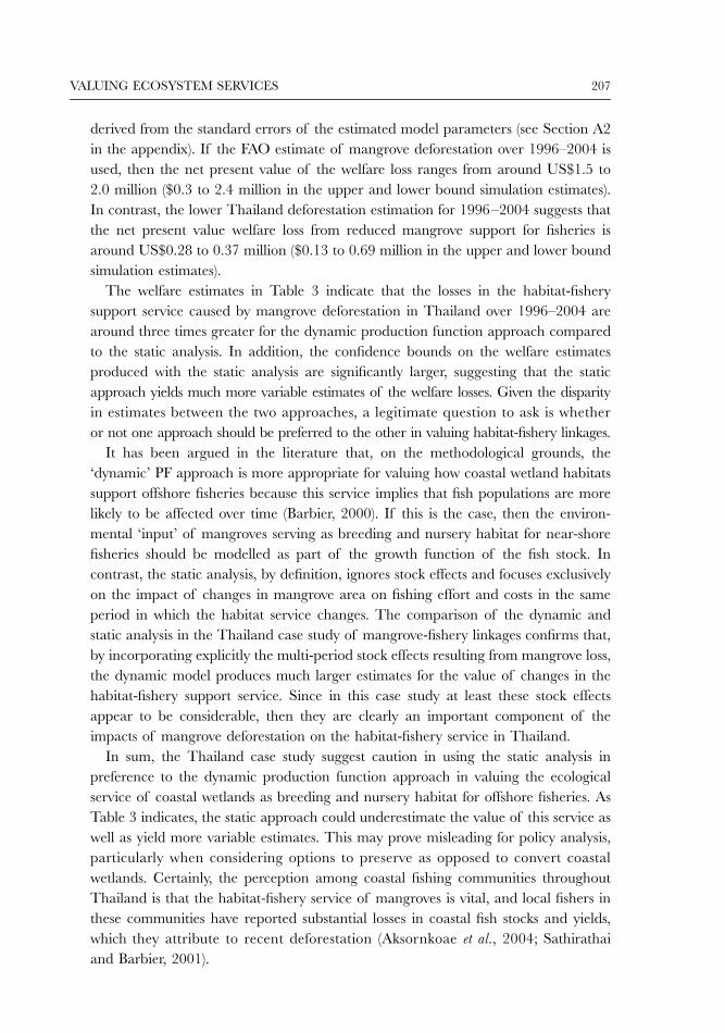
VALUING ECOSYSTEM SERVICES 207
derived from the standard errors of the estimated model parameters (see Section A2in the appendix). If the FAO estimate of mangrove deforestation over 1996–2004 isused, then the net present value of the welfare loss ranges from around US$1.5 to2.0 million ($0.3 to 2.4 million in the upper and lower bound simulation estimates).In contrast, the lower Thailand deforestation estimation for 1996–2004 suggests thatthe net present value welfare loss from reduced mangrove support for fisheries isaround US$0.28 to 0.37 million ($0.13 to 0.69 million in the upper and lower boundsimulation estimates).
The welfare estimates in Table 3 indicate that the losses in the habitat-fisherysupport service caused by mangrove deforestation in Thailand over 1996–2004 arearound three times greater for the dynamic production function approach comparedto the static analysis. In addition, the confidence bounds on the welfare estimatesproduced with the static analysis are significantly larger, suggesting that the staticapproach yields much more variable estimates of the welfare losses. Given the disparityin estimates between the two approaches, a legitimate question to ask is whetheror not one approach should be preferred to the other in valuing habitat-fishery linkages.
It has been argued in the literature that, on the methodological grounds, the‘dynamic’ PF approach is more appropriate for valuing how coastal wetland habitatssupport offshore fisheries because this service implies that fish populations are morelikely to be affected over time (Barbier, 2000). If this is the case, then the environ-mental ‘input’ of mangroves serving as breeding and nursery habitat for near-shorefisheries should be modelled as part of the growth function of the fish stock. Incontrast, the static analysis, by definition, ignores stock effects and focuses exclusivelyon the impact of changes in mangrove area on fishing effort and costs in the sameperiod in which the habitat service changes. The comparison of the dynamic andstatic analysis in the Thailand case study of mangrove-fishery linkages confirms that,by incorporating explicitly the multi-period stock effects resulting from mangrove loss,the dynamic model produces much larger estimates for the value of changes in thehabitat-fishery support service. Since in this case study at least these stock effectsappear to be considerable, then they are clearly an important component of theimpacts of mangrove deforestation on the habitat-fishery service in Thailand.
In sum, the Thailand case study suggest caution in using the static analysis inpreference to the dynamic production function approach in valuing the ecologicalservice of coastal wetlands as breeding and nursery habitat for offshore fisheries. AsTable 3 indicates, the static approach could underestimate the value of this service aswell as yield more variable estimates. This may prove misleading for policy analysis,particularly when considering options to preserve as opposed to convert coastalwetlands. Certainly, the perception among coastal fishing communities throughoutThailand is that the habitat-fishery service of mangroves is vital, and local fishers inthese communities have reported substantial losses in coastal fish stocks and yields,which they attribute to recent deforestation (Aksornkoae et al., 2004; Sathirathaiand Barbier, 2001).
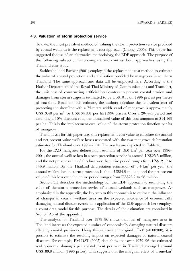
208 EDWARD B. BARBIER
4.3. Valuation of storm protection service
To date, the most prevalent method of valuing the storm protection service providedby coastal wetlands is the replacement cost approach (Chong, 2005). This paper hassuggested the use of an alternative methodology, the EDF approach. The purpose ofthe following subsection is to compare and contrast both approaches, using theThailand case study.
Sathirathai and Barbier (2001) employed the replacement cost method to estimatethe value of coastal protection and stabilization provided by mangroves in southernThailand. The same approach and data will be employed here. According to theHarbor Department of the Royal Thai Ministry of Communications and Transport,the unit cost of constructing artificial breakwaters to prevent coastal erosion anddamages from storm surges is estimated to be US$1011 (in 1996 prices) per metreof coastline. Based on this estimate, the authors calculate the equivalent cost ofprotecting the shoreline with a 75-metre width stand of mangrove is approximatelyUS$13.48 per m2, or US$134 801 per ha (1996 prices). Over a 20-year period andassuming a 10% discount rate, the annualized value of this cost amounts to $14 169per ha. This is the ‘replacement cost’ value of the storm protection function per haof mangrove.
The analysis for this paper uses this replacement cost value to calculate the annualand net present value welfare losses associated with the two mangrove deforestationestimates for Thailand over 1996–2004. The results are depicted in Table 4.
For the FAO mangrove deforestation estimate of 18.0 km2 per year over 1996–2004, the annual welfare loss in storm protection service is around US$25.5 million,and the net present value of this loss over the entire period ranges from US$121.7 to146.9 million. For the Thailand deforestation estimation of 3.4 km2 per year, theannual welfare loss in storm protection is about US$4.9 million, and the net presentvalue of this loss over the entire period ranges from US$23.2 to 28 million.
Section 3.5 describes the methodology for the EDF approach to estimating thevalue of the storm protection service of coastal wetlands such as mangroves. Asemphasized in the appendix, the key step to this approach is to estimate the influenceof changes in coastal wetland area on the expected incidence of economicallydamaging natural disaster events. The application of the EDF approach here employsa count data model for this purpose. The details of the estimation are contained inSection A3 of the appendix.
The analysis for Thailand over 1979–96 shows that loss of mangrove area inThailand increases the expected number of economically damaging natural disastersaffecting coastal provinces. Using this estimated ‘marginal effect’ (−0.00308), it ispossible to estimate the resulting impact on expected damages of natural coastaldisasters. For example, EM-DAT (2005) data show that over 1979–96 the estimatedreal economic damages per coastal event per year in Thailand averaged aroundUS$189.9 million (1996 prices). This suggests that the marginal effect of a one-km2
VALUING ECOSYSTEM SERVICES 209
loss of mangrove area is an increase in expected storm damages of about US$585 000per km2. In Table 4, this latter calculation is combined with the FAO and Thailandestimates of the average annual rates of deforestation to compute the welfare lossesin storm protection service for Thailand over 1996–2004. The table shows the wel-fare calculations based both on the point estimates of the count data regression andon using the standard errors to construct 95% confidence bounds on these estimates.
Table 4 shows that, for the FAO mangrove deforestation estimate of 18.0 km2 peryear over 1996–2004, the EDF approach estimates the annual welfare loss in stormprotection service to be around US$3.4 million ($2.3 to 5.8 million with 95% confi-dence), and the net present value of this loss over the entire period ranges fromUS$16.1 to 19.5 million ($11.2 to 33.4 million with 95% confidence). For the Thai-land deforestation estimation of 3.4 km2 per year, the annual welfare loss in stormprotection is over US$0.65 million ($0.45 to 1.1 million with 95% confidence), andthe net present value of this loss over the entire period ranges from US$3.1 to 3.7million ($2.1 to 6.4 million with 95% confidence).
Comparing the EDF approach and the replacement cost method of estimating thewelfare impacts of a loss of the storm protection service due to mangrove deforestationconfirms that the replacement cost method tends to produce extremely highestimates – almost 4 times greater than even the largest upper-bound estimate
Table 4. Valuation of storm protection service, Thailand, 1996–2004 (US$)
Valuation approach Average annual mangrove loss
FAO (18.0 km2)a Thailand (3.44 km2)b
Replacement cost method:c
Annual welfare loss 25 504 821 4 869 720Net present value (10% discount rate) 146 882 870 28 044 836Net present value (12% discount rate) 135 896 056 25 947 087Net present value (15% discount rate) 121 698 392 23 236 280
Expected damage function approach:Annual welfare loss 3 382 169 645 769
( 2 341 686–5 797 339) (447 106–1 106 905)Net present value 19 477 994 3 718 998(10% discount rate) (13 485 827–33 387 014) (2 574 894–6 374 694)Net present value 18 021 043 3 440 818(12% discount rate) (12 477 089–30 889 671) (2 382 292–5 897 868)Net present value 16 138 305 3 081 340(15% discount rate) (11 173 553–27 662 490) (2 133 404–5 281 692)
Notes: Figures in parentheses represent upper and lower bound welfare estimates based on the 95% confidenceinterval for the estimated coefficients in the model (see Section A3 in the appendix).a FAO estimates from FAO (2003). 2000 and 2004 data are estimated from 1990–2000 annual average mangroveloss of 18.0 km2.b Thailand estimates from various Royal Thailand Forestry Department sources reported in Aksornkoae andTokrisna (2004). 2000 and 2004 data are estimated from 1993–96 annual average mangrove loss of 3.44 km2
c Re-calculated based on Sathirathai and Barbier (2001).
Sources: Author’s calculations.
210 EDWARD B. BARBIER
calculated using the EDF approach. This suggests that the replacement cost methodshould be used with caution, and when data are available, the EDF approach mayprovide more reliable values of the storm protection service of coastal wetlands.
4.4. Land use policy implications
Valuation of the ecosystem services provided by mangroves are important for twoland use policy decisions in Thailand. First, although declining in recent years, con-version of remaining mangroves to shrimp farm ponds and other commercial coastaldevelopments continues to be a major threat to Thailand’s remaining mangroveareas. Second, since the December 2004 tsunami disaster, there is now considerableinterest in rehabilitating and restoring mangrove ecosystems as ‘natural barriers’ tofuture coastal storm events.
To illustrate how improved and more accurate valuation of ecosystems can helpinform these two policy decisions, Table 5 compares the per hectare net returns toshrimp farming, the costs of mangrove rehabilitation and the value of mangroveservices. All land uses are assumed to be instigated over 1996–2004 and are valuedin 1996 US dollars. The net economic returns to shrimp farming are based on non-declining yields over a 5-year period of investment, with the pond abandoned insubsequent years (Sathirathai and Barbier, 2001). These returns to shrimp aquacultureare estimated to be $1078 to $1220 per ha. In comparison, the costs rehabilitatingmangrove ecosystems on land that has been converted to shrimp farms and thenabandoned are $8812 to $9318 per ha. Thus valuing the goods and services ofmangrove ecosystems can help to address two important policy questions: Do the neteconomic returns to shrimp farming justify further mangrove conversion to this economicactivity, and is it worth investing in mangrove replanting and ecosystem rehabilitationin abandoned shrimp farm areas?
As indicated in Table 5, if the older methods of valuing habitat-fishery linkageswith the static approach and storm protection with the replacement cost method areemployed, then mangrove ecosystem benefits are considerably higher than the neteconomic returns to shrimp farming and the costs of replanting and rehabilitatingmangroves in abandoned farm areas. However, the static analysis undervalues thehabitat-fishery linkage of mangroves whereas the replacement cost method over-inflates storm protection. The replacement cost method estimates storm protectionat $67 610 to 81 602 per ha, which is 99% of the value of all mangrove ecosystembenefits. In contrast, the net income to local coastal communities from collected forestproducts and the value of habitat-fishery linkages total to only $730 to $881 per ha,which suggests that these two benefits of mangroves are insufficient on their own tojustify either halting conversion to shrimp farms or replanting and rehabilitating theseecosystems on abandoned pond land.
If improved methods of valuing habitat-fishery linkages by the dynamic approachand storm protection by the expected damage function method are employed, then
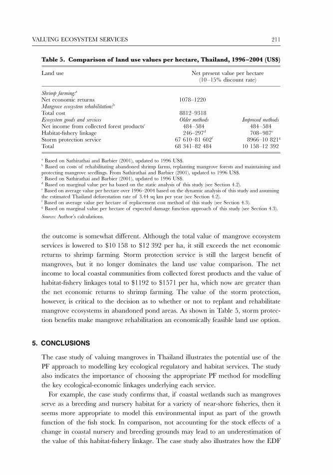
VALUING ECOSYSTEM SERVICES 211
the outcome is somewhat different. Although the total value of mangrove ecosystemservices is lowered to $10 158 to $12 392 per ha, it still exceeds the net economicreturns to shrimp farming. Storm protection service is still the largest benefit ofmangroves, but it no longer dominates the land use value comparison. The netincome to local coastal communities from collected forest products and the value ofhabitat-fishery linkages total to $1192 to $1571 per ha, which now are greater thanthe net economic returns to shrimp farming. The value of the storm protection,however, is critical to the decision as to whether or not to replant and rehabilitatemangrove ecosystems in abandoned pond areas. As shown in Table 5, storm protec-tion benefits make mangrove rehabilitation an economically feasible land use option.
5. CONCLUSIONS
The case study of valuing mangroves in Thailand illustrates the potential use of thePF approach to modelling key ecological regulatory and habitat services. The studyalso indicates the importance of choosing the appropriate PF method for modellingthe key ecological-economic linkages underlying each service.
For example, the case study confirms that, if coastal wetlands such as mangrovesserve as a breeding and nursery habitat for a variety of near-shore fisheries, then itseems more appropriate to model this environmental input as part of the growthfunction of the fish stock. In comparison, not accounting for the stock effects of achange in coastal nursery and breeding grounds may lead to an underestimation ofthe value of this habitat-fishery linkage. The case study also illustrates how the EDF
Table 5. Comparison of land use values per hectare, Thailand, 1996–2004 (US$)
Land use Net present value per hectare (10–15% discount rate)
Shrimp farming:a
Net economic returns 1078–1220Mangrove ecosystem rehabilitation:b
Total cost 8812–9318Ecosystem goods and services Older methods Improved methodsNet income from collected forest productsc 484–584 484–584Habitat-fishery linkage 246–297d 708–987e
Storm protection service 67 610–81 602f 8966–10 821g
Total 68 341–82 484 10 158–12 392
a Based on Sathirathai and Barbier (2001), updated to 1996 US$.b Based on costs of rehabilitating abandoned shrimp farms, replanting mangrove forests and maintaining andprotecting mangrove seedlings. From Sathirathai and Barbier (2001), updated to 1996 US$.c Based on Sathirathai and Barbier (2001), updated to 1996 US$.d Based on marginal value per ha based on the static analysis of this study (see Section 4.2).e Based on average value per hectare over 1996–2004 based on the dynamic analysis of this study and assuming the estimated Thailand deforestation rate of 3.44 sq km per year (see Section 4.2).f Based on average value per hectare of replacement cost method of this study (see Section 4.3).g Based on marginal value per hectare of expected damage function approach of this study (see Section 4.3).
Sources: Author’s calculations.
212 EDWARD B. BARBIER
approach can be applied to valuing the storm protection service provided by mangroves,and demonstrates why this method should be preferred to the less-reliable replacementcost method, which has been used extensively in the literature to date (Chong, 2005).
The case study also points to some important policy implications for Thailand. Inrecent decades, considerable mangrove deforestation has taken place in Thailand, mainlyas a result of shrimp farm expansion and other coastal economic developments (see Figure 4).Over this period, mangrove conversion for these development activities was system-atically encouraged by government land use policies (Aksornkoae and Tokrisna, 2004;Barbier, 2003; Sathirathai and Barbier, 2001). Such policies were designed withoutconsideration of the value of the ecological services provided by mangroves, such astheir habitat support for coastal fisheries and storm protection. The case study of valuingthese ecological services for Thailand illustrates that their benefits are significant, andshould certainly not be ignored in future mangrove land management decisions.
The case study applications in this paper of valuing coastal storm protection andhabitat services have policy implications beyond Thailand as well. Even beforeHurricanes Katrina and Rita devastated the central Gulf Coast of the United Statesin 2005, the US Army Corps of Engineers had proposed a $1.1 billion multi-yearprogramme to slow the rate of wetland loss and restore some wetlands in coastalLouisiana. In the aftermath of these hurricanes, the US Congress is now consideringexpanding the programme substantially to a $14 billion restoration effort (Zinn,2005). As noted in Section 4, in the wake of the 2004 Asian tsunami, mangroverestoration projects for enhanced coastal protection are underway in many countriesthroughout the region. International donor groups are also supporting mangroverestoration projects in Asia, especially in countries and regions devastated by thetsunami (Check, 2005). In addition, there is mounting scientific evidence that near-shore fisheries throughout the world are undergoing rapid decline, with loss of coastalhabitat and nursery grounds for these fisheries a contributory cause ( Jackson et al.,2001; Myers and Worm, 2003). Valuing the storm protection and habitat services ofcoastal wetlands, as illustrated by the Thailand case study in this paper, can thereforeplay a vital role in current and future debates about the state of coastal ecosystemsworldwide and the assessment of the costs and benefits of restoring these vital ecosystems.
Thus, valuing the non-market benefits of ecological regulatory and habitat servicesis becoming increasingly important in assisting policymakers to manage criticalenvironmental assets. However, further progress applying production functionapproaches and other methods to value ecological services faces two challenges.
First, for these methods to be applied effectively to valuing ecosystem services, it is importantthat the key ecological and economic relationships are well understood. Unfortunately,our knowledge of the ecological functions, let alone the ecosystem processes andcomponents, underlying many of the services listed in Table 1 is still incomplete.
Second, natural ecosystems are subject to stresses, rapid change and irreversiblelosses, they tend to display threshold effects and other non-linearities that are difficultto predict, let alone model in terms of their economic impacts. These uncertainties
VALUING ECOSYSTEM SERVICES 213
can affect the estimation of values from an ex ante (‘beforehand’) perspective. Theeconomic valuation literature recognizes that such uncertainties create the conditionsfor option values, which arise from the difference between valuation under conditionsof certainty and uncertainty (e.g., see Freeman, 2003 and Just et al., 2004). Thestandard approach recommended in the literature is to estimate this additional valueseparately, through various techniques to measure an option price, that is, the amountof money that an individual will pay or must be compensated to be indifferent fromthe status quo condition of the ecosystem and the new, proposed condition. However,in practice, estimating separate option prices for unknown ecological effects is verydifficult. Determining the appropriate risk premium for vulnerable populationsexposed to the irreversible ecological losses is also proving elusive. These are problemscurrently affecting all economic valuation methods of ecosystem services, and not justthe production function approach. As one review of these studies concludes: ‘Giventhe imperfect knowledge of the way people value natural ecosystems and theirgoods and services, and our limited understanding of the underlying ecology andbiogeochemistry of aquatic ecosystems, calculations of the value of the changesresulting from a policy intervention will always be approximate’ (Heal et al., 2005, p. 218).
Finally, Section 3 noted recent attempts to extend the production functionapproach to the ecosystem level through integrated ecological-economic modelling.This allows the ecosystem functioning and dynamics underlying the provision ofecological services to be modelled and can be used to value multiple rather thansingle services. For example, returning to the Thailand case study, it is well knownthat both coral reefs and sea grasses complement the role of mangroves in providingboth the habitat-fishery and storm protection services. Thus full modelling of theintegrated mangrove–coral reef–sea grass system could improve measurement of thebenefits of both services. As we learn more about the important ecological andeconomic role played by such services, it may be relevant to develop multi-serviceecosystem modelling to understand more fully what values are lost when suchintegrated coastal and marine systems are disturbed or destroyed.
Discussion
Carlo A. FaveroIGIER, Bocconi University and CEPR
The objective of the paper is to apply a production function (and expected damage)approach to ‘valuing the environment as input’, with an application to a mangroveecosystem in Thailand. I shall concentrate my discussion only on the productionfunction approach, but the main methodological points raised are naturally extendedto the expected damage function approach.
214 EDWARD B. BARBIER
An environmental good or service essentially serves as a factor input into productionthat yields utility. The fundamental problem of the empirical application is theevaluation of the following value function:
where B is the social benefits in any time period of the mangrove ecosystem, and r isthe discount rate.
There are two fundamental questions:1. What is the appropriate discount rate?2. How to evaluate B?
The first question is not explicitly addressed and different scenarios on the discountrate are adopted; the production function approach is the answer to the second question.
In theory the production function approach can be described as follows:
• Specification of a dynamic intertemporal optimization problem, where one of theconstraints is the production function relating the input of interest to the measurableoutput.
• Solution of the model.
• Identification and estimation (or, whenever estimation is not possible, calibration) ofthe technology and preference parameters of the model and of the auxiliary parameters.
• Dynamic stochastic simulation of the model to derive EtBt+j and the associatedconfidence intervals.
In practice two alternative approaches are considered: a static one and a dynamicone. I shall not comment on the static approach because I find this inappropriate tothe very nature of the problem at hand, which is, by definition, dynamic.
In the dynamic approach a model is postulated to determine the dynamics of thestock of fish measured in biomass units, Xt, the fishing effort, Et, the landed fish priceper unit harvested, p, and the harvest, h. The adopted model is described as follows:
where F(Xt, St) is biological growth in the current period, which is a function of St, themangrove area, h(Xt, Et), harvesting is a function of the stock as well as fishing effort,Et. Fishing effort is modelled as a partial adjustment model in which the equilibriumvalue is determined by fish price per unit harvested and the unit cost of effort, w.
V EB
rt tt j
jj
T
( )
=+
+
=∑ 10
X X F X S h X E
E E p h w E
F X S rXX
S
h qX E
p kh
t t t t t t
t t t t t t
t t tt
t
t t t
t t
+
+
− = −
− = −
= −
=
=
1
1
1
( , ) ( , )
[ ]
( , ) ln
φ
α
η
VALUING ECOSYSTEM SERVICES 215
The model is estimated and then simulated keeping w exogenous and taking alter-native scenarios for S, that by consequence is taken as exogenous. Using someassumption for the discount rate the present value of a reduction in the mangrovearea is then computed.
The results are interesting but there are a number of important questions that themodelling strategy leaves open:
• In the dynamic model S is exogenous and no law of motion for S is specified. Themodel is not capable of explaining the reduction in S that we observe in the data.In fact, if agents were acting following this model we would have never observeda reduction in S, because a reduction in S has only costs and no benefits.Macroeconometricians might see the applicability of the Lucas critique to thismodel as an immediate consequence of the assumption of exogeneity of S.
• Expectations do not explicitly enter the model.
• What are the costs incurred in omitting from the model the dynamics of w?
• What is the performance of this model when evaluated in sample by dynamicsimulation?
• How is uncertainty added for estimation and more importantly for dynamicsimulation? The result reported in Table 4 seems to take account of only coefficientuncertainty while, given the modelling choices, the fluctuations in the relevant variablesnot explained by the adopted model are likely to be the main source of uncertainty.
I think that the answer to this set of open questions could further enhance thepotential of the interesting methods for valuing ecosystem services very well discussedin this paper.
Omer MoavHebrew University, University of London Royal Holloway, Shalem Center, and CEPR
Edward Barbier demonstrates how basic micro theory can be implemented toestimate the value of ecological services for human welfare. In particular, two methodsare developed: the production function approach and the expected damage functionapproach. Both methods utilize exogenous variation in the size of the ecosystemservice, such as the size of a mangrove forest, on a beneficial outcome. According tothe former the outcome is welfare gained from the decline in the price of a consumptiongood, such as fish, that utilizes the ecosystem as an input in its production process.In the latter it is the economic value of the reduction in damage, arising, for instance,from storms, that is reduced by a larger ecosystem.
The theory is rather straightforward. It is the availability of the data that theestimation depends on, and it is not clear that for most practical problems there existssufficient exogenous variation in the ecosystem, allowing for a reliable assessment.Nevertheless, Barbier convincingly illustrates that despite the difficulties, these methodshave the potential to provide important information about the value of the ecosystem
216 EDWARD B. BARBIER
and thereby the value of preventing its disappearance. This information can becomecritical for policymakers, and might, even if only in marginal cases, generate thecrucial political force to reverse processes of natural habitat destruction.
The value of the functions of the ecosystem include, as stated by Barbier, ‘climatestability, maintenance of biodiversity and beneficial species, erosion control, floodmitigation, storm protection, groundwater recharge and pollution control’. Thisstatement reveals another limitation of the estimation methods. It focuses on a limitedset of benefits, implying a potentially huge underestimation of the value of theecosystem. First, due to information problems regarding most functions, it is difficultto identify the size of the impact and/or its welfare value. For instance, most likelyexogenous variety in the ecosystem is not sufficient to estimate its effect on climatestability, and the welfare value of biodiversity is a question hard to answer.
Second, the cost of preserving the ecosystem – giving up the benefits of itsalternative use – is paid by the local population, while many of its services extendbeyond that. As is well known, preserving natural ecosystems is a problem with largeexternalities that go beyond borders. In other words, who cares? Do we expect thepoor fisherman in Thailand, or their government, to allocate a significant weight inits welfare function to biodiversity? In fact, it is the population of the developed worldthat cares, and this population’s willingness to pay a compensating price, could beabove and beyond the benefit of the ecosystem to the local population.
A more technical comment on the estimation process regards the open accessassumption and, in particular, the implicit assumption that changes in the habitat aresufficiently small, relative to the economy, such that the producer’s surplus isunchanged. Welfare gains from a larger ecosystem emerge only from the reductionin consumer goods prices. This assumption adds to the bias in the estimation,reducing the value of the ecosystem. To see this point, suppose that prices of theconsumption good are also given (traded good in an open economy). In this casethere is zero welfare gain from preserving the environment.
A final comment about the estimation method regards the implicit assumption ofstability of the steady-state equilibrium. However, non-monotonic convergence to thesteady state might characterize the dynamics of the ecosystem. For instance, thepopulation of a species might converge to its steady state in oscillations, implying thata negative shock to the ecosystem might, once it is sufficiently fragile, result in extinctionof a species rather than a proportional reduction in the size of the natural population.
Beyond the problems of estimating the direct value of the ecological services forhuman welfare, lies a somewhat deeper question regarding the long-run effects of theutilization of natural resources for the benefit of mankind in the production process.Maintaining natural habitats and benefiting their production services, or destroyingthem and benefiting from their alternative land use for agriculture, might have differentlong-run consequences on demographic variables, institutional development, and, inparticular, human capital promoting institutions (e.g., public schools, loans, and childlabour regulation), and the resulting accumulation of human capital.
VALUING ECOSYSTEM SERVICES 217
Natural resources, according to many studies, are a hurdle for the process ofdevelopment, in particular the accumulation of human capital. (e.g. Gylfason, 2001).But to the best of my knowledge, we do not know yet how to make a distinction inthat regard between an open-access preserved ecosystem and agricultural land.Therefore, depleting resources or increasing the size of agricultural land on theaccount of the ecosystem, could have a significant impact on the economy.
Moreover, the transition from an open access ecosystem into private owned farmlandmight have an impact on wealth inequality, in particular inequality in the ownershipof such land. Deninger and Squire (1998) show that inequality in land ownership hasa negative impact on economic growth. Engerman and Sokoloff (2000) provide evidencethat wealth inequality, brought about oppressive institutions (e.g., restricted access tothe democratic process and to education). They argue that these institutions weredesigned to maintain the political power of the elite and to preserve the existinginequality. Galor et al. (2005) provide evidence that inequality in the ownership ofagricultural land has a negative effect on public expenditure on education, and arguethat the elite of landowners might prevent public schooling, despite the support of theowners of capital and the working class.
On the other hand, if the destruction of the ecosystem increases farmland andthereby possibly promoting industrial development, and if the process does notgenerate large wealth inequality, the return to human capital will most likely rise.This could trigger a process of development stemming from reduced fertility andincreased investment in education. This brings us back to the main problem ofpreventing the distractions of an ecosystem: the externality. Each small economymight be better-off destroying the ecosystem, giving rise to an inefficient equilibrium.The analysis suggested by Barbier, could, at least, highlight the benefits of preservingnatural habitats for the local economy.
APPENDIX: APPLICATION TO THAILAND CASE STUDY
This appendix outlines the econometric estimations for valuing habitat-fishery linkagesand the storm protection service of mangroves in the Thailand case study of Section 4.
A1. Static valuation of habitat-fishery linkage
To apply the static analysis of habitat-fishery linkages of Section 3.3.1 to the Thailandcase study, it is necessary to estimate the unknown parameters (A, a, b) of the log-linear version of the Cobb–Douglas production function:
ln hit = A0 + a ln Eit + b ln Mit + µit (A1)
where i = 1, . . . , 5 zones, t = 1, . . . , 14 years (1983–96) and A0 = ln A.Equation (A1) was estimated using the pooled data on demersal fisheries, shellfish
and mangrove area from Barbier (2003). These were the data on harvest, hit, and
218 EDWARD B. BARBIER
effort, Eit, for Thailand’s shellfish and demersal fisheries, as well as mangrove area,Mit across the five coastal zones of Thailand and over the years1983–96. Variousregression procedures for a pooled data set were utilized and compared, including:(i) ordinary least squares (OLS); (ii) one- and two-way panel analysis of fixed andrandom effects; and (iii) a maximum likelihood estimation by an iterated generalizedleast squares (GLS) procedure for a pooled time series and cross-sectional regression,which allows for correction of any groupwise heteroscedasticity, cross-group correlationand common or within-group autocorrelation. Table A1 indicates the best regressionmodel for the shellfish and demersal fisheries respectively, and the relevant test statistics.
For demersal fisheries, the preferred model shown in Table A1 is the GLS estimationallowing for groupwise heteroscedasticity and correcting for both cross-group andcommon autocorrelation. For the panel analysis of the demersal fisheries, the likelihoodratio tests of the null hypothesis of zero individual and time effects across all five zonesand fourteen time periods were significant, thus rejecting the null hypothesis. Inaddition, the Breusch–Pagan Lagrange multiplier (LM) statistic was also significant atthe 95% confidence level for both the one-way and two-models, which suggestsrejection of the null hypothesis of zero random disturbances. The Hausman teststatistic was also significant at the 99% confidence level, suggesting that the fixedeffects specification is preferred to the random effects. However, in both the one- andtwo-way fixed effects model the t-test on the estimated parameter for a in Equation(A1) was insignificant, suggesting the null hypothesis that a = 0 cannot be rejected.As indicated in Table A1, from the pooled time series cross-sectional GLS regressionfor demersal fisheries, the likelihood ratio (LR) test statistic of the null hypothesis forhomoscedasticity based on the least squares regression was computed to be 24.64,which is statistically significant. Although not shown in the table, the alternative Waldtest for homoscedasticity is also statistically significant and confirms rejection of thenull hypothesis. Thus the GLS model with correction of groupwise heteroscedasticityis preferred to the OLS regression. The LM statistic of 14.43 also reported in TableA1 for demersal fisheries is a test of the null hypothesis of zero cross-sectional correlation,which proves to be statistically significant. Although not indicated in the table, theLR test statistic for groupwise heteroscedasticity as a restriction on cross-groupcorrelation was estimated to be 23.26, which is also statistically significant. Thus thenull hypothesis of zero cross-group correlation in the demersal fisheries regression canbe rejected. The common autocorrelation coefficient across all five zones was estimatedto be 0.484, and as shown in Table A1, once the GLS model for demersal fish wascorrected for this common autocorrelation, the null hypothesis that the coefficient a= 0 is now rejected.
For shellfish, as indicated in Table A1 the preferred estimation of Equation (A1) isthe GLS estimation allowing for groupwise heteroscedasticity and correcting forcross-group correlation, with A0 restricted to zero. For the panel analysis of shellfish,the likelihood ratio tests and Breusch–Pagan LM tests of the null hypothesis of noindividual and time effects were significant, thus rejecting the null hypothesis. The
VALUING ECOSYSTEM SERVICES 219
Hausman test statistic was significant, suggesting that the fixed effects specification ispreferred to the random effects. However, in both the one- and two-way fixed effectsmodel the t-test on the estimated parameters for a and b in Equation (A1) wasinsignificant, suggesting the null hypothesis a = b = 0 cannot be rejected. As indicatedin Table A1, from the pooled time series cross-sectional GLS regression of shellfish,the LR test statistic of the null hypothesis for homoscedasticity based on the leastsquares regression is 35.08, which is statistically significant. Although not shown inthe table, the alternative Wald test for homoscedasticity is also statistically significantand confirms rejection of the null hypothesis. Thus the GLS model with correctionof groupwise heteroscedasticity is preferred to the OLS regression. The LM statisticof 21.30 also reported in Table A1 for the shellfish regression is a test of the nullhypothesis of zero cross-sectional correlation, which proves to be statistically signifi-cant. Although not indicated in the table, the LR test statistic for groupwise hetero-scedasticity as a restriction on cross-group correlation was estimated to be 43.90,which is also statistically significant. Thus the null hypothesis of zero cross-groupcorrelation in the shellfish regression can be rejected. As shown in Table A1, oncethe GLS model of shellfish was corrected for groupwise heteroscedasticity and corre-lation, the null hypotheses that a = 0 and b = 0 are now rejected.
The estimations of Equation (A1) for Thailand’s shellfish and demersal fisherieswere used in conditions (5) and (6) to calculate the welfare impacts of mangrovedeforestation over 1996–2004 on Thailand’s artisanal fisheries. The analysis uses thesame iso-elastic demand function as in Barbier (2003), with a demand elasticity, ε,of −0.5. The results are reported in Table 3, which shows welfare calculations forboth the point estimates and upper and lower bounds on these estimates based onthe standard errors of the regression coefficients reported in Table A1.
Table A1. Estimates of Equation (A1) for Thailand’s shellfish and demersal fisheries
Coefficient Demersal fisherya Shellfish fisheryb
A0 11.213 (24.568)** –A 0.341 (4.992)** 1.688 (38.254)**B 0.100 (2.763)** 0.196 (3.693)**Log-likelihoodc 5.401 –71.517Likelihood ratio statisticd 24.643** 35.076**Lagrange multiplier statistice 14.426* 21.304**
Notes: t-statistics are shown in parentheses.a Preferred model is groupwise heteroscedastic and correlated GLS, corrected for common autocorrelation.b Preferred model is groupwise heteroscedastic and correlated GLS, with A0 restricted to zero.c In the demersal fishery regression, correction of cross-group correlation Cov[eit,ejt] = σij leads to a positivelog-likelihood.d Tests the null hypothesis of homoscedasticity based on OLS.e Tests the null hypothesis of zero cross-group correlation based on OLS.* Significant at 95% confidence level.** Significant at 99% confidence level.
Sources: Author’s estimations.
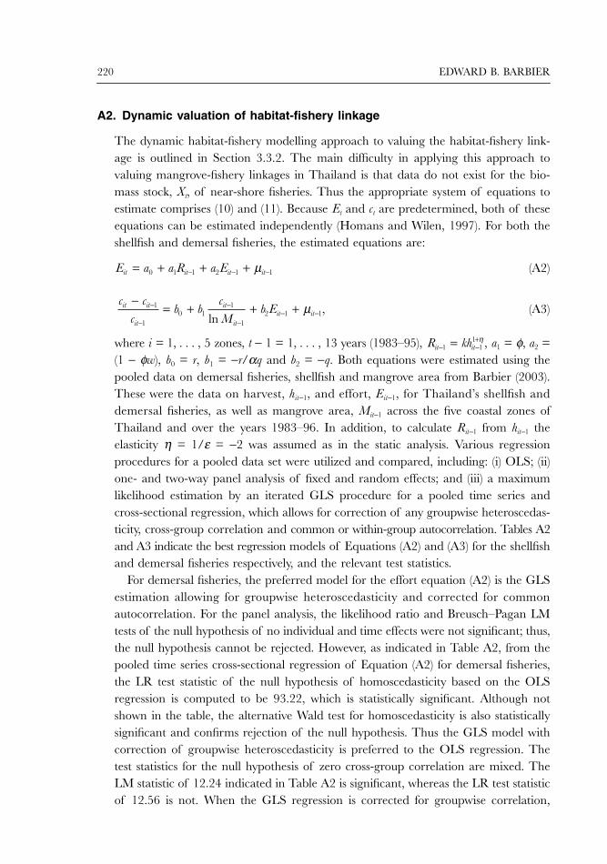
220 EDWARD B. BARBIER
A2. Dynamic valuation of habitat-fishery linkage
The dynamic habitat-fishery modelling approach to valuing the habitat-fishery link-age is outlined in Section 3.3.2. The main difficulty in applying this approach tovaluing mangrove-fishery linkages in Thailand is that data do not exist for the bio-mass stock, Xt, of near-shore fisheries. Thus the appropriate system of equations toestimate comprises (10) and (11). Because Et and ct are predetermined, both of theseequations can be estimated independently (Homans and Wilen, 1997). For both theshellfish and demersal fisheries, the estimated equations are:
(A2)
(A3)
where i = 1, . . . , 5 zones, t − 1 = 1, . . . , 13 years (1983–95), a1 = φ, a2 =(1 − φw), b0 = r, b1 = −r/αq and b2 = −q. Both equations were estimated using thepooled data on demersal fisheries, shellfish and mangrove area from Barbier (2003).These were the data on harvest, hit−1, and effort, Eit−1, for Thailand’s shellfish anddemersal fisheries, as well as mangrove area, Mit−1 across the five coastal zones ofThailand and over the years 1983–96. In addition, to calculate Rit−1 from hit−1 theelasticity η = 1/ε = −2 was assumed as in the static analysis. Various regressionprocedures for a pooled data set were utilized and compared, including: (i) OLS; (ii)one- and two-way panel analysis of fixed and random effects; and (iii) a maximumlikelihood estimation by an iterated GLS procedure for a pooled time series andcross-sectional regression, which allows for correction of any groupwise heteroscedas-ticity, cross-group correlation and common or within-group autocorrelation. Tables A2and A3 indicate the best regression models of Equations (A2) and (A3) for the shellfishand demersal fisheries respectively, and the relevant test statistics.
For demersal fisheries, the preferred model for the effort equation (A2) is the GLSestimation allowing for groupwise heteroscedasticity and corrected for commonautocorrelation. For the panel analysis, the likelihood ratio and Breusch–Pagan LMtests of the null hypothesis of no individual and time effects were not significant; thus,the null hypothesis cannot be rejected. However, as indicated in Table A2, from thepooled time series cross-sectional regression of Equation (A2) for demersal fisheries,the LR test statistic of the null hypothesis of homoscedasticity based on the OLSregression is computed to be 93.22, which is statistically significant. Although notshown in the table, the alternative Wald test for homoscedasticity is also statisticallysignificant and confirms rejection of the null hypothesis. Thus the GLS model withcorrection of groupwise heteroscedasticity is preferred to the OLS regression. Thetest statistics for the null hypothesis of zero cross-group correlation are mixed. TheLM statistic of 12.24 indicated in Table A2 is significant, whereas the LR test statisticof 12.56 is not. When the GLS regression is corrected for groupwise correlation,
E a a R a Eit it it it = + + +− − −0 1 1 2 1 1µ
c cc
b bcM
b Eit it
it
it
itit it
ln ,
−= + + +−
−
−
−− −
1
10 1
1
12 1 1µ
R khit it− −+=1 1
1 ,η
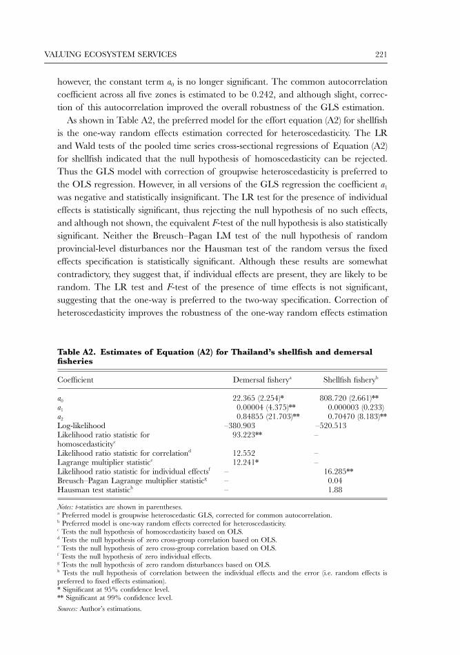
VALUING ECOSYSTEM SERVICES 221
however, the constant term a0 is no longer significant. The common autocorrelationcoefficient across all five zones is estimated to be 0.242, and although slight, correc-tion of this autocorrelation improved the overall robustness of the GLS estimation.
As shown in Table A2, the preferred model for the effort equation (A2) for shellfishis the one-way random effects estimation corrected for heteroscedasticity. The LRand Wald tests of the pooled time series cross-sectional regressions of Equation (A2)for shellfish indicated that the null hypothesis of homoscedasticity can be rejected.Thus the GLS model with correction of groupwise heteroscedasticity is preferred tothe OLS regression. However, in all versions of the GLS regression the coefficient a1
was negative and statistically insignificant. The LR test for the presence of individualeffects is statistically significant, thus rejecting the null hypothesis of no such effects,and although not shown, the equivalent F-test of the null hypothesis is also statisticallysignificant. Neither the Breusch–Pagan LM test of the null hypothesis of randomprovincial-level disturbances nor the Hausman test of the random versus the fixedeffects specification is statistically significant. Although these results are somewhatcontradictory, they suggest that, if individual effects are present, they are likely to berandom. The LR test and F-test of the presence of time effects is not significant,suggesting that the one-way is preferred to the two-way specification. Correction ofheteroscedasticity improves the robustness of the one-way random effects estimation
Table A2. Estimates of Equation (A2) for Thailand’s shellfish and demersal fisheries
Coefficient Demersal fisherya Shellfish fisheryb
a0 22.365 (2.254)* 808.720 (2.661)**a1 0.00004 (4.375)** 0.000003 (0.233)a2 0.84855 (21.703)** 0.70470 (8.183)**Log-likelihood –380.903 –520.513Likelihood ratio statistic for 93.223** –homoscedasticityc
Likelihood ratio statistic for correlationd 12.552 –Lagrange multiplier statistice 12.241* –Likelihood ratio statistic for individual effectsf – 16.285**Breusch–Pagan Lagrange multiplier statisticg – 0.04Hausman test statistich – 1.88
Notes: t-statistics are shown in parentheses.a Preferred model is groupwise heteroscedastic GLS, corrected for common autocorrelation.b Preferred model is one-way random effects corrected for heteroscedasticity.c Tests the null hypothesis of homoscedasticity based on OLS.d Tests the null hypothesis of zero cross-group correlation based on OLS.e Tests the null hypothesis of zero cross-group correlation based on OLS.f Tests the null hypothesis of zero individual effects.g Tests the null hypothesis of zero random disturbances based on OLS.h Tests the null hypothesis of correlation between the individual effects and the error (i.e. random effects ispreferred to fixed effects estimation).* Significant at 95% confidence level.** Significant at 99% confidence level.
Sources: Author’s estimations.
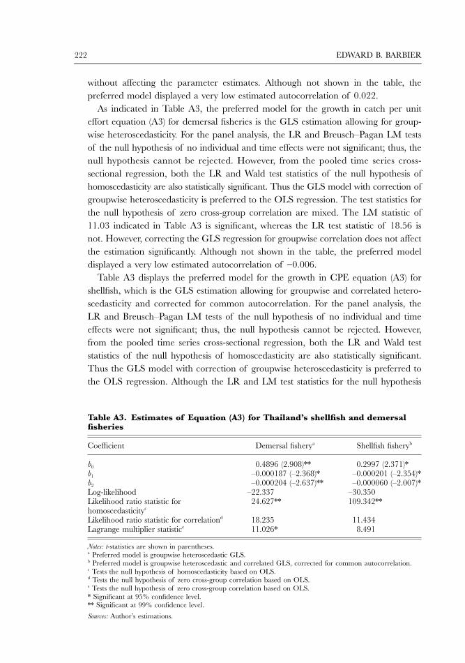
222 EDWARD B. BARBIER
without affecting the parameter estimates. Although not shown in the table, thepreferred model displayed a very low estimated autocorrelation of 0.022.
As indicated in Table A3, the preferred model for the growth in catch per uniteffort equation (A3) for demersal fisheries is the GLS estimation allowing for group-wise heteroscedasticity. For the panel analysis, the LR and Breusch–Pagan LM testsof the null hypothesis of no individual and time effects were not significant; thus, thenull hypothesis cannot be rejected. However, from the pooled time series cross-sectional regression, both the LR and Wald test statistics of the null hypothesis ofhomoscedasticity are also statistically significant. Thus the GLS model with correction ofgroupwise heteroscedasticity is preferred to the OLS regression. The test statistics forthe null hypothesis of zero cross-group correlation are mixed. The LM statistic of11.03 indicated in Table A3 is significant, whereas the LR test statistic of 18.56 isnot. However, correcting the GLS regression for groupwise correlation does not affectthe estimation significantly. Although not shown in the table, the preferred modeldisplayed a very low estimated autocorrelation of −0.006.
Table A3 displays the preferred model for the growth in CPE equation (A3) forshellfish, which is the GLS estimation allowing for groupwise and correlated hetero-scedasticity and corrected for common autocorrelation. For the panel analysis, theLR and Breusch–Pagan LM tests of the null hypothesis of no individual and timeeffects were not significant; thus, the null hypothesis cannot be rejected. However,from the pooled time series cross-sectional regression, both the LR and Wald teststatistics of the null hypothesis of homoscedasticity are also statistically significant.Thus the GLS model with correction of groupwise heteroscedasticity is preferred tothe OLS regression. Although the LR and LM test statistics for the null hypothesis
Table A3. Estimates of Equation (A3) for Thailand’s shellfish and demersal fisheries
Coefficient Demersal fisherya Shellfish fisheryb
b0 0.4896 (2.908)** 0.2997 (2.371)*b1 –0.000187 (–2.368)* –0.000201 (–2.354)*b2 –0.000204 (–2.637)** –0.000060 (–2.007)*Log-likelihood –22.337 –30.350Likelihood ratio statistic for 24.627** 109.342**homoscedasticityc
Likelihood ratio statistic for correlationd 18.235 11.434Lagrange multiplier statistice 11.026* 8.491
Notes: t-statistics are shown in parentheses.a Preferred model is groupwise heteroscedastic GLS.b Preferred model is groupwise heteroscedastic and correlated GLS, corrected for common autocorrelation.c Tests the null hypothesis of homoscedasticity based on OLS.d Tests the null hypothesis of zero cross-group correlation based on OLS.e Tests the null hypothesis of zero cross-group correlation based on OLS.* Significant at 95% confidence level.** Significant at 99% confidence level.
Sources: Author’s estimations.
VALUING ECOSYSTEM SERVICES 223
of zero cross-group correlation are not significant, correcting the GLS regression forgroupwise correlation improves the significance confidence level of the estimatedparameter b2 from 90 to 95%. The common autocorrelation coefficient across all fivezones is estimated to be 0.147, and although slight, correction of this autocorrelationimproved the overall robustness of the GLS estimation.
Using the estimated parameters for Equations (A2) and (A3) for Thailand’s shellfishand demersal fisheries allows simulation of the welfare impacts of mangrove deforestationover 1996–2004 on Thailand’s artisanal fisheries. Again, the same demand functionwith elasticity of −0.5 as in Barbier (2003) is employed. The results are reported inTable 3, which shows welfare calculations for both the point estimates and upper andlower bounds on these estimates based on the standard errors of the regressioncoefficients reported in Tables A2 and A3.
A3. Expected damage function valuation of storm protection service
As discussed in Section 3.5, the key step in applying the expected damage functionapproach to valuing the storm protection service of a coastal wetland such as mangrovesis to estimate how a change in mangrove area influences the expected incidence ofeconomically damaging natural disaster events.
Suppose that for a number of coastal regions, i = 1, . . . , N, and over a given periodof time, t = 1, . . . , T the ith coastal region could experience in any period t any numberof zit = 0, 1, 2, 3 . . . economically damaging storm event incidents. A common assumptionin count data models is that the count variable zit has a Poisson distribution, in whichcase the expected number of storm events in each region per period is given by:
(A4)
where as before, Sit is the area of wetlands, xit, are other factors, and αi accounts forother possible ‘unobserved’ effects on the incidence of disasters specific to eachcoastal region. Estimation of βS, along with an estimate of the conditional mean λit,allows ∂Ζ/∂S in Equation (13) to be determined. One drawback of the Poisson dis-tribution (Equation (A4)) is that it automatically implies ‘equidispersion’, that is, theconditional variance of zit is also equal to λit. To test whether this is the case, thePoisson method of estimating (A4) should be compared to other techniques, such asthe Negative Binomial model, which do not assume equidispersion in the variance of zit.
For the Thailand case study, the estimation of (A4) is:
ln E[zit|Mit, xit] = ln λit = αi + βSMit + β′xit + µit, (A5)
where i = 1, . . . , 21 coastal provinces, t = 1, . . . , 18 years (1979–96). The EM-DAT(2005) International Disaster Database contains data on the number of coastal disas-ters occurring in Thailand since 1975 and the approximate location and date of itsimpacts. From these data it is possible to determine zit, the number of economically
E z s x eE z S x
Sit it it itS x it it it
itit S
i S it it[ | , ] , [ | , ]
= = =+ + ′λ ∂∂
λ βα β β
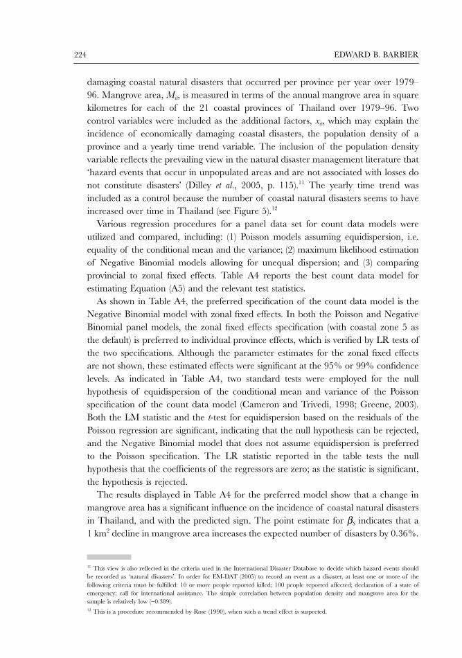
224 EDWARD B. BARBIER
damaging coastal natural disasters that occurred per province per year over 1979–96. Mangrove area, Mit, is measured in terms of the annual mangrove area in squarekilometres for each of the 21 coastal provinces of Thailand over 1979–96. Twocontrol variables were included as the additional factors, xit, which may explain theincidence of economically damaging coastal disasters, the population density of aprovince and a yearly time trend variable. The inclusion of the population densityvariable reflects the prevailing view in the natural disaster management literature that‘hazard events that occur in unpopulated areas and are not associated with losses donot constitute disasters’ (Dilley et al., 2005, p. 115).11 The yearly time trend wasincluded as a control because the number of coastal natural disasters seems to haveincreased over time in Thailand (see Figure 5).12
Various regression procedures for a panel data set for count data models wereutilized and compared, including: (1) Poisson models assuming equidispersion, i.e.equality of the conditional mean and the variance; (2) maximum likelihood estimationof Negative Binomial models allowing for unequal dispersion; and (3) comparingprovincial to zonal fixed effects. Table A4 reports the best count data model forestimating Equation (A5) and the relevant test statistics.
As shown in Table A4, the preferred specification of the count data model is theNegative Binomial model with zonal fixed effects. In both the Poisson and NegativeBinomial panel models, the zonal fixed effects specification (with coastal zone 5 asthe default) is preferred to individual province effects, which is verified by LR tests ofthe two specifications. Although the parameter estimates for the zonal fixed effectsare not shown, these estimated effects were significant at the 95% or 99% confidencelevels. As indicated in Table A4, two standard tests were employed for the nullhypothesis of equidispersion of the conditional mean and variance of the Poissonspecification of the count data model (Cameron and Trivedi, 1998; Greene, 2003).Both the LM statistic and the t-test for equidispersion based on the residuals of thePoisson regression are significant, indicating that the null hypothesis can be rejected,and the Negative Binomial model that does not assume equidispersion is preferredto the Poisson specification. The LR statistic reported in the table tests the nullhypothesis that the coefficients of the regressors are zero; as the statistic is significant,the hypothesis is rejected.
The results displayed in Table A4 for the preferred model show that a change inmangrove area has a significant influence on the incidence of coastal natural disastersin Thailand, and with the predicted sign. The point estimate for βS indicates that a1 km2 decline in mangrove area increases the expected number of disasters by 0.36%.
11 This view is also reflected in the criteria used in the International Disaster Database to decide which hazard events shouldbe recorded as ‘natural disasters’. In order for EM-DAT (2005) to record an event as a disaster, at least one or more of thefollowing criteria must be fulfilled: 10 or more people reported killed; 100 people reported affected; declaration of a state ofemergency; call for international assistance. The simple correlation between population density and mangrove area for thesample is relatively low (−0.389).12 This is a procedure recommended by Rose (1990), when such a trend effect is suspected.
VALUING ECOSYSTEM SERVICES 225
It is likely that the mangrove loss in Thailand, especially since the mid-1970s (seeFigure 4), has increased the expected number of economically damaging coastalnatural disasters per year. The estimated marginal effect corresponding to βS of achange in mangrove area on coastal natural disasters (−0.0031) can be employed toestimate the resulting impact of mangrove deforestation over 1979–96 in Thailandon expected damages of natural coastal disasters. This is described further in Section4.3 and shown in Table 4.
As discussed in Section 3.5, an underlying hypothesis of the expected damagefunction methodology is that, if coastal wetland loss increases the incidence of naturaldisaster per year, then wetland loss is also associated with increasing storm damages.However, under certain circumstances the results of a count data model could provide amisleading test of this null hypothesis. For instance, suppose a loss in wetland area isassociated with a change in the incidence of storms from one devastating storm totwo relatively minor storms per year. The count data model would then be inter-preted as not providing evidence against the null that the change in the wetland areaincreases expected storm damages, when what has actually happened is that totalstorm damages have declined over time with wetland loss. This suggests the need fora robustness check on the count data model, such as Equation (A5) in the Thailandcase study, to ensure that such situations do not dominate the application of the EDFapproach.
One possible robustness check is to test the null hypothesis directly; that is, are totaldamages from storm events increasing with coastal wetland loss? In the Thailand casestudy, the relevant estimation is
Table A4. Negative binomial estimation of Equation (A5) with zonal fixed effects
Variable Parameter estimatea Marginal effectb
Mangrove area (Mit) –0.0036 (–4.448)** –0.0031 (–2.745)**Population density (POPDENit) –0.0005 (–1.079) –0.0004 (–0.894)Annual time trend (YRTRNit) 0.0781 (5.558)** 0.0669 (2.615)**Dispersion parameter (αit) 0.0001Estimated conditional mean (λ) 0.8559Log-likelihood –373.66Lagrange multiplier statisticc 39.967**Regression t-testd –5.385**Likelihood ratio statistice 74.919**
Notes: t-statistics shown in parentheses.a Parameter estimates for the zonal fixed effects are not shown. Zone 5 is the default and the fixed effects forzones 1 to 4 were negative and significant at the 95% or 99% confidence levels.b Estimate of λitβ3 (see Equation (A4)).c Tests the null hypothesis of equidispersion in the Poisson model.d A regression-based test of the null hypothesis of equidispersion in the Poisson model.e Tests the null hypothesis that the restricted regression without the explanatory variables Mit, POPDENit andYRTRNit is the preferred Negative Binomial model with zonal fixed effects.* Significant at 95% confidence level.** Significant at 99% confidence level.
Sources: Author’s estimations.
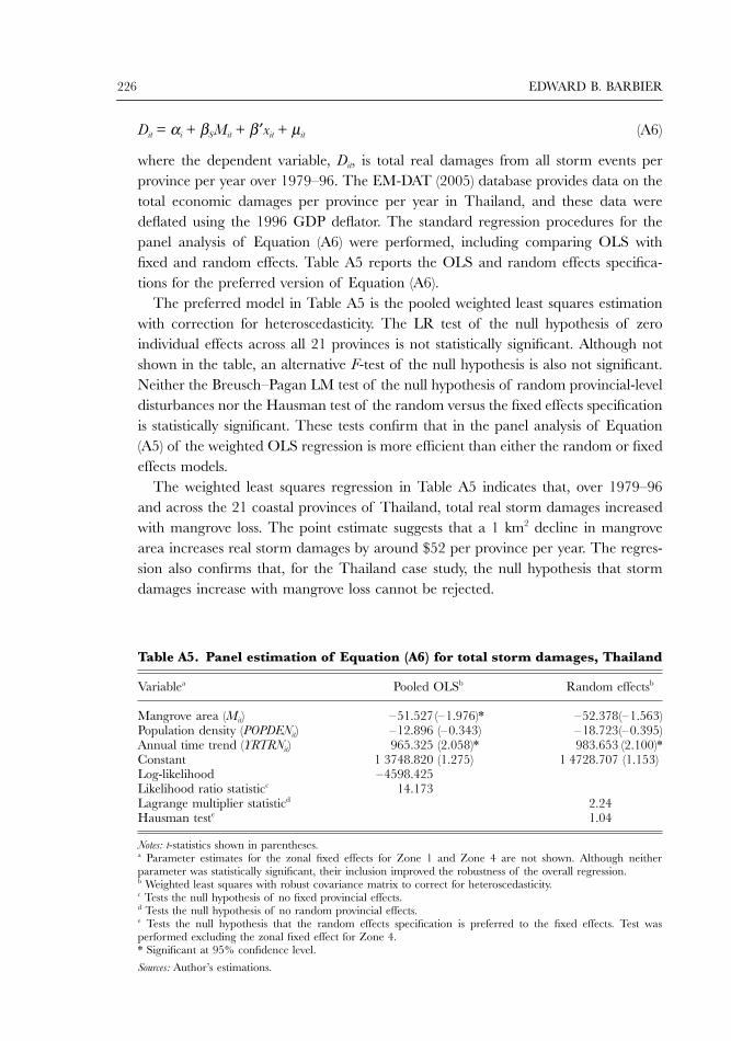
226 EDWARD B. BARBIER
Dit = αi + βSMit + β′xit + µit (A6)
where the dependent variable, Dit, is total real damages from all storm events perprovince per year over 1979–96. The EM-DAT (2005) database provides data on thetotal economic damages per province per year in Thailand, and these data weredeflated using the 1996 GDP deflator. The standard regression procedures for thepanel analysis of Equation (A6) were performed, including comparing OLS withfixed and random effects. Table A5 reports the OLS and random effects specifica-tions for the preferred version of Equation (A6).
The preferred model in Table A5 is the pooled weighted least squares estimationwith correction for heteroscedasticity. The LR test of the null hypothesis of zeroindividual effects across all 21 provinces is not statistically significant. Although notshown in the table, an alternative F-test of the null hypothesis is also not significant.Neither the Breusch–Pagan LM test of the null hypothesis of random provincial-leveldisturbances nor the Hausman test of the random versus the fixed effects specificationis statistically significant. These tests confirm that in the panel analysis of Equation(A5) of the weighted OLS regression is more efficient than either the random or fixedeffects models.
The weighted least squares regression in Table A5 indicates that, over 1979–96and across the 21 coastal provinces of Thailand, total real storm damages increasedwith mangrove loss. The point estimate suggests that a 1 km2 decline in mangrovearea increases real storm damages by around $52 per province per year. The regres-sion also confirms that, for the Thailand case study, the null hypothesis that stormdamages increase with mangrove loss cannot be rejected.
Table A5. Panel estimation of Equation (A6) for total storm damages, Thailand
Variablea Pooled OLSb Random effectsb
Mangrove area (Mit) –51.527 (–1.976)* –52.378 (–1.563)Population density (POPDENit) –12.896 (–0.343) –18.723 (–0.395)Annual time trend (YRTRNit) 965.325 (2.058)* 983.653 (2.100)*Constant 1 3748.820 (1.275) 1 4728.707 (1.153)Log-likelihood –4598.425Likelihood ratio statisticc 14.173Lagrange multiplier statisticd 2.24Hausman teste 1.04
Notes: t-statistics shown in parentheses.a Parameter estimates for the zonal fixed effects for Zone 1 and Zone 4 are not shown. Although neitherparameter was statistically significant, their inclusion improved the robustness of the overall regression.b Weighted least squares with robust covariance matrix to correct for heteroscedasticity.c Tests the null hypothesis of no fixed provincial effects.d Tests the null hypothesis of no random provincial effects.e Tests the null hypothesis that the random effects specification is preferred to the fixed effects. Test wasperformed excluding the zonal fixed effect for Zone 4.* Significant at 95% confidence level.
Sources: Author’s estimations.
VALUING ECOSYSTEM SERVICES 227
REFERENCES
Acharya, G. and E.B. Barbier (2000). ‘Valuing groundwater recharge through agriculturalproduction in the Hadejia-Jama’are wetlands in northern Nigeria’, Agricultural Economics, 22,247–59.
Aksornkoae, S. and R. Tokrisna (2004). ‘Overview of shrimp farming and mangrove loss inThailand’, in E.B. Barbier and S. Sathirathai (eds.), Shrimp Farming and Mangrove Loss inThailand, Edward Elgar, London.
Aksornkoae, S., R. Tokrisna, W. Sugunnasil and S. Sathirathai (2004). ‘The importance ofmangroves: Ecological perspectives and socio-economic values’, in E.B. Barbier and S.Sathirathai (eds.), Shrimp Farming and Mangrove Loss in Thailand, Edward Elgar, London.
Barbier, E.B. (1994). ‘Valuing environmental functions: Tropical wetlands’, Land Economics,70(2), 155–73.
— (2000). ‘Valuing the environment as input: Applications to mangrove-fishery linkages’,Ecological Economics, 35, 47–61.
— (2003). ‘Habitat-fishery linkages and mangrove loss in Thailand’, Contemporary EconomicPolicy, 21(1), 59–77.
Barbier, E.B. and M. Cox (2003). ‘Does economic development lead to mangrove loss? Across-country analysis’, Contemporary Economic Policy, 21(4), 418–32.
Barbier, E.B. and S. Sathirathai (eds.) (2004). Shrimp Farming and Mangrove Loss in Thailand.Edward Elgar, London.
Barbier, E.B. and I. Strand (1998). ‘Valuing mangrove-fishery linkages: A case study ofCampeche, Mexico’, Environmental and Resource Economics, 12, 151–66.
Barbier, E.B., I. Strand and S. Sathirathai (2002). ‘Do open access conditions affect thevaluation of an externality? Estimating the welfare effects of mangrove-fishery linkages’,Environmental and Resource Economics, 21(4), 343–67.
Bjørndal, T. and J.M. Conrad (1987). ‘The dynamics of an open access fishery’, CanadianJournal of Economics, 20, 74–85.
Boscolo, M. and J.R. Vincent (2003). ‘Nonconvexities in the production of timber, biodiversity,and carbon sequestration’, Journal of Environmental Economics and Management, 46, 251–68.
Cameron, C.A. and P. Trivedi (1998). Regression Analysis of Count Data, Cambridge UniversityPress, Cambridge.
Carlsson, F., P. Frykblom and C. Lijenstolpe (2003). ‘Valuing wetland attributes: An applica-tion of choice experiments’, Ecological Economics, 47, 95–103.
Carpenter, S.R., D. Ludwig and W.A. Brock (1999). ‘Management of eutrophication for lakessubject to potentially irreversible change’, Ecological Applications, 9(3), 751–71.
Charuppat, T. and J. Charuppat (1997). The Use of Landsat-5 (TM) Satellite Images for Tracing theChanges of Mangrove Forest Areas of Thailand, Royal Forestry Department, Bangkok.
Check, E. (2005). ‘Roots of recovery’, Nature, 438, 910–11.Chong, J. (2005). Protective Values of Mangrove and Coral Ecosystems: A Review of Methods and Evidence,
IUCN, Gland, Switzerland.Clark, C. (1976). Mathematical Bioeconomics, John Wiley and Sons, New York.Dahdouh-Guebas, F., L.P. Jayatissa, D. Di Nitto, J.O. Bosire, D. Lo Seen and N. Koedam (2005). ‘How
effective were mangroves as a defence against the recent tsunami?’ Current Biology, 15(12), 443–47.Daily, G. (ed.) (1997). Nature’s Services: Societal Dependence on Natural Ecosystems, Island Press,
Washington DC.De Groot, R.S., M.A. Wilson and R.M.J. Boumans (2002). ‘A typology for the classification,
description and valuation of ecosystem functions, goods and services’, Ecological Economics,41, 393–408.
Deninger, K. and L. Squire (1998). ‘New ways of looking at old issues: Inequality and growth’,Journal of Development Economics, 57, 259–87.
Dickie, M. (2003). ‘Defensive behavior and damage cost methods’, in P. Champ, K.J. Boyleand T.C. Brown (eds.), A Primer on Nonmarket Valuation, Kluwer, Boston, MA.
Dilley, M., R.S. Chen, U. Deichmann, A.L. Lerner-Lam and M. Arnold (2005). Natural DisasterHotspots: A Global Risk Analysis. Disaster Risk Management Series, Hazard ManagementUnit, The World Bank, Washington, DC.
Ellis, G.M. and A.C. Fisher (1987). ‘Valuing the environment as input’, Journal of EnvironmentalManagement, 25, 149–56.
228 EDWARD B. BARBIER
EM-DAT (2005). EM-DAT: The OFDA/CRED International Disaster Database. www.em-dat.net,Université Catholique de Louvain, Brussels, Belgium.
Engerman, S. and Sokoloff, K.L. (2000). ‘Factor endowment, inequality, and paths of developmentamong new world economies’, UCLA.
FAO (2003). ‘Status and trends in mangrove area extent worldwide’ (by M.L. Wilkie and S.Fortuna) Forest Resources Assessment Working Paper No. 63, Forest Resources Division,Food and Agricultural Organization of the United Nations, Rome.
Finnoff, D. and J. Tschirhart (2003). ‘Harvesting in an eight-species ecosystem’, Journal ofEnvironmental Economics and Management, 45, 589–611.
Freeman, A.M. III. (1982). Air and Water Pollution Control: A Benefit-Cost Assessment, John Wiley,New York.
— (1991). ‘Valuing environmental resources under alternative management regimes’, EcologicalEconomics, 3, 247–56.
— (2003). The Measurement of Environmental and Resource Values: Theory and Methods, 2nd edn,Resources for the Future, Washington DC.
Galor, O., O. Moav and D. Vollrath (2005). ‘Inequality in land ownership, the emergence ofhuman capital promoting institutions, and the great divergence’, Brown University.
Greene, W.H. (2003). Econometric Analysis, 5th edn, Prentice-Hall, Englewood Cliffs, NJ.Gren, I-M., K. Elofsson and P. Jannke (1997). ‘Cost-effective nutrient reductions to the Baltic
Sea’, Environmental and Resource Economics, 10, 341–62.Gylfason, T. (2001). ‘Natural resources, education, and economic development’, European
Economic Review, 45, 847–59.Harakunarak, A. and S. Aksornkoae (2005). ‘Life-saving belts: Post-tsunami reassessment of
mangrove ecosystem values and management in Thailand’, Tropical Coasts, July, 48–55.Heal, G.M., E.B. Barbier, K.J. Boyle, A.P. Covich, S.P. Gloss, C.H. Hershner, J.P. Hoehn,
C.M. Pringle, S. Polasky, K. Segerson and K. Shrader-Frechette (2005). Valuing Ecosystem Services:Toward Better Environmental Decision Making, The National Academies Press, Washington DC.
Hirshleifer, J. and J.G. Riley (1992). The Analytics of Uncertainty and Information, CambridgeUniversity Press, Cambridge.
Homans, F.R. and J.E. Wilen (1997). ‘A model of regulated open access resource use’, Journalof Environmental Economics and Management, 32, 1–21.
Jackson, J.B.C., M.X. Kirby, W.H. Berger, et al. (2001). ‘Historical overfishing and the recentcollapse of coastal ecosystems’, Science, 293, 629–38.
Just, R.E., D.L. Hueth and A. Schmitz (2004). The Welfare Economics of Public Policy: A PracticalApproach to Project and Policy Evaluation, Edward Elgar, Cheltenham, UK.
Kahn, J.R., and W.M. Kemp (1985). ‘Economic losses associated with the degradation of anecosystem: The case of submerged aquatic vegetation in Chesapeake Bay’, Journal of Envi-ronmental Economics and Management, 12, 246–63.
Kaiser, B. and J. Roumasset (2002). ‘Valuing indirect ecosystem services: The case of tropicalwatersheds’, Environment and Development Economics, 7, 701–14.
Kaosa-ard, M. and S. Pednekar (1998). ‘Background Report for the Thai Marine RehabilitationPlan 1997–2001’, Report submitted to the Joint Research Centre of the Commission of theEuropean Communities and the Department of Fisheries, Ministry of Agriculture andCooperatives, Thailand, Thailand Development Research Institute, Bangkok.
Kathiresan, K. and N. Rajendran (2005). ‘Coastal mangrove forests mitigated tsunami’,Estuarine Coastal and Shelf Science, 65, 601–606.
Knowler, D., E.B. Barbier, and I. Strand (2001). ‘An open-access model of fisheries andnutrient enrichment in the Black Sea’, Marine Resource Economics, 16, 195–217.
Krutilla, J.V. and A.C. Fisher (1985). The Economics of Natural Environments: Studies in the Valuationof Commodity and Amenity Resources, Resources for the Future, Washington, DC.
Lynne, G.D., P. Conroy and F.J. Prochaska (1981). ‘Economic value of marsh areas for marineproduction processes’, Journal of Environmental Economics and Management, 8, 175–86.
Mardle, S., C. James, C. Pipitone and M. Kienzle (2004). ‘Bioeconomic interactions in anestablished fishing exclusion zone: The Gulf of Castellammare, NW Sicily’, Natural ResourceModeling, 17(4), 393–447.
Massel, S.R., K. Furukawa and R.M. Brinkman (1999). ‘Surface wave propagation data inmangrove forests’, Fluid Dynamics Research, 24, 219–49.
Mazda, Y., E. Wolanski, B. King, A. Sase, D. Ohtsuka and M. Magi (1997). ‘Drag force dueto vegetation in mangrove swamps’, Mangroves and Salt Marshes, 1, 193–99.
VALUING ECOSYSTEM SERVICES 229
McConnell, K.E. and I.E. Strand (1989). ‘Benefits from commercial fisheries when demand andsupply depend on water quality’, Journal of Environmental Economics and Management, 17, 284–92.
Michener, R. and C. Tighe (1992). ‘A Poisson regression model of highway fatalities’, AmericanEconomic Review, 82(2), 452–56.
Millennium Ecosystem Assessment (2003). Ecosystems and Human Well-being: A Framework forAssessment, Island Press, Washington DC.
Mitsch, W.J. and J.G. Gosselink (1993). Wetlands, 2nd edn, Van Norstrand Reinhold, New York.Myers, R.A. and B. Worm (2003). ‘Rapid worldwide depletion of predatory fish communities’,
Nature, 423, 280–83.Naylor, R. and M. Drew (1998). ‘Valuing mangrove resources in Kosrae, Micronesia’, Environ-
ment and Development Economics, 3, 471–90.Olson, M.K. (2004). ‘Are novel drugs more risky for patients than less novel drugs?’ Journal of
Health Economics, 23, 1135–58.Pagiola, S., K. von Ritter and J. Bishop (2004). How Much is an Ecosystem Worth? Assessing the
Economic Value of Conservation, The World Bank, Washington DC.Parks, P. and M. Bonfaz (1997). ‘Nonsustainable use of renewable resources: Mangrove
deforestation and mariculture in Ecuador’, Marine Resource Economics, 9, 1–18.Ready, R.C. (1995). ‘Environmental valuation under uncertainty’, in D.W. Bromley (ed.), The
Handbook of Environmental Economics, Blackwell Publishers, Cambridge, MA, pp. 568–93.Ricketts, T.H., G.C. Daily, P.R. Ehrlich and C.D. Michener (2004). ‘Economic value of tropical
forest to coffee production’, Proceedings of the National Academy of Science, 101(304), 12579–82.Rodwell, L.D., E.B. Barbier, C.M. Roberts and T.R. McClanahan (2002). ‘A model of tropical
marine reserve-fishery linkages’, Natural Resource Modeling, 15(4), 453–86.Rose, N.L. (1990). ‘Profitability and product quality: Economic determinants of airline safety
performance’, Journal of Political Economy, 98(5), 944–64.Sathirathai, S. and E.B. Barbier (2001). ‘Valuing mangrove conservation in Southern
Thailand’, Contemporary Economic Policy, 19, 109–22.Schnute, J. (1977). ‘Improved estimates of the Schaefer Production Model: Theoretical
considerations’, Journal of the Fisheries Research Board of Canada, 34, 583–603.Settle, C. and J.F. Shogren (2002). ‘Modeling native-exotic species within Yellowstone Lake’,
American Journal of Agricultural Economics, 84(5), 1323–28.Shabman, L.A. and S.S. Batie (1978). ‘Economic value of natural coastal wetlands: A critique’,
Coastal Zone Management Journal, 4(3), 231–47.Sugunnasil, W. (1998). ‘Fishing communities and coastal resource management in Southern
Thailand’, mimeo, Department of Social Sciences, Prince of Songkla University, Pattani, Thailand.Sumaila, U.R. (2002). ‘Marine protected area performance in a model of a fishery’, Natural
Resource Modeling, 15(4), 439–51.Swallow, S.K. (1994). ‘Renewable and nonrenewable resource theory applied to coastal
agriculture, forest, wetland and fishery linkages’, Marine Resource Economics, 9, 291–310.UNEP (United Nations Environment Program) (2005). After the Tsunami: Rapid Environmental
Assessment Report, UNEP, Nairobi, 22 February; www.unep.org/tsunami/reports.Valiela, I., J.L. Bowen and J.K. York (2001). ‘Mangrove forests: One of the world’s threatened
major tropical environments’, BioScience, 51(10), 807–15.Wattana, S. (1998). ‘Fishing Communities and Coastal Resource Management in Southern Thai-
land’. Mimeo. Department of Social Sciences, Prince of Songkla University, Pattani, Thailand.Wetlands International (2005). Natural Mitigation of Natural Disasters. Assessment Report to
Ramsar STRP12, Wetlands International, Jakarta, 2 February.Winkelmann, R. (2003). Econometric Analysis of Count Data, 4th edn, Springer-Verlag, Berlin.World Conservation Monitoring Centre (WCMC) (1992). ‘Wetlands’, in WCMC (ed.), Global
Biodiversity: Status of the Earth’s Living Resources, IUCN, Gland, Switzerland.World Resources Institute (WRI) (1996). World Resources 1996–7, World Resources Institute,
Washington DC.— (2001). World Resources 2000–2001. People and Ecosystems: The Fraying Web of Life, World
Resources Institute, Washington DC.Wu, J., K. Skelton-Groth, W.G. Boggess and R.M. Adams (2003). ‘Pacific salmon restoration: Trade-offs
between economic efficiency and political acceptance’, Contemporary Economic Policy, 21(1), 78–89.Zinn, J. (2005). Hurricanes Katrina and Rita and the Coastal Louisiana Ecosystem Restoration. CRS
Report for Congress, The Congressional Research Service, The Library of Congress,Washington DC, 26 September.