valuing product innovation: genetically engineered
TRANSCRIPT

RAND Journal of EconomicsVol. 50, No. 3, Fall 2019pp. 615–644
Valuing product innovation: geneticallyengineered varieties in US corn and soybeans
Federico Ciliberto∗GianCarlo Moschini∗∗and
Edward D. Perry∗∗∗
We develop a discrete-choice model of differentiated products for US corn and soybean seeddemand to study the welfare impact of genetically engineered (GE) crop varieties. Using a uniquedata set spanning the period 1996–2011, we find that the welfare impact of the GE innovation issignificant. In the last five years of the period analyzed, our preferred counterfactual indicates thattotal surplus due to GE traits was $5.18 billion per year, with seed manufacturers appropriating56% of this surplus. The seed industry obtained more surplus from GE corn, whereas farmersreceived more surplus from GE soybeans.
1. Introduction
� Innovation, in the form of new and improved crop varieties, has long played a critical role inthe quest to ensure sufficient food supply for a rapidly growing world population. Conventionalbreeding activities have led to remarkable successes, such as hybrid maize (Griliches, 1957) andthe green revolution (Evenson and Gollin, 2003). Genetically engineered (GE) crop varietiesbuild on this tradition by exploiting the recombinant DNA tools of modern biotechnology. Firstintroduced commercially in 1996, by most standards, GE varieties have been very successful(Moschini, 2008). Despite being essentially limited to four main crops (maize, soybean, cotton,and canola), as of 2017, GE varieties were grown on more than 469 million acres worldwide. TheUnited States has been at the forefront of these developments: in 2017, GE varieties were plantedon more than 183 million acres of US farmland, nearly 91% of which was maize and soybeans(ISAAA, 2017).
∗ University of Virginia, CEPR, London, and DIW, Berlin; [email protected].∗∗ Iowa State University; [email protected].∗∗∗ Kansas State University; [email protected] thank two anonymous referees and Editor Chad Syverson for helpful comments and suggestions. This research wassupported by the National Institute of Food and Agriculture, US Department of Agriculture, grant no. 2015-67023-22954.Ciliberto also thanks the Bankard Fund for Political Economy at the University of Virginia for financial support, andMoschini gratefully acknowledges the support of the Pioneer Endowed Chair in Science and Technology Policy at IowaState University.
C© 2019, The RAND Corporation. 615
616 / THE RAND JOURNAL OF ECONOMICS
Notwithstanding their productivity-enhancing potential, GE crops have been highly contro-versial. Concerns raised include the fear that GE products are harmful to human health and/or theenvironment, and ethical objections related to human manipulation of the DNA of living plantsand animals. Many of these concerns have been allayed (Bennett et al., 2013). In particular, theenvironmental impacts of GE varieties appear to be generally positive (NRC, 2010; Barrows,Sexton, and Zilberman, 2014; Perry, Moschini, and Hennessy, 2016). However, a separate per-sistent source of public mistrust relates to the ownership interests of multinational corporationsthat commercialize GE products. Unlike innovations underpinning the green revolution, whichwere largely the result of publicly sponsored research and development (R&D) activities (Wright,2012), GE crop varieties have been primarily developed by private firms, with US seed companies(Monsanto in primis) at the forefront. The proprietary nature of GE technologies, and an ongoingconsolidation of the seed and agrochemical industry, has heightened concerns about the pricingof these new products, their contribution to welfare, and the actual beneficiaries of the innovation(Clancy and Moschini, 2017).
In this article, we provide novel econometric evidence on the welfare effects of the introduc-tion of GE crop varieties. We draw on a large, proprietary data set of plot-level seed choices bya representative sample of US farmers for the two most important GE crops, corn and soybeans.The data span the period from 1996 (the year GE corn and soybean varieties were first introduced)to 2011 (by which time the average adoption rate of GE varieties exceeded 90%), and containinformation on the specific seed products that farmers buy—brand, amount bought, area planted,price paid, and which (if any) GE traits are included in the seed. The richness of the data allowsus to estimate an explicit structural model of farmers’ demand for seed varieties rooted in thetheory of discrete choice in a differentiated product setting (Anderson, De Palma, and Thisse,1992). Although this model pertains to a production input (seeds) used by competitive firms,rather than consumer products, it is nonetheless in the tradition of the empirical industrial orga-nization (IO) literature on demand estimation in industries with differentiated products (Berry,1994; Goldberg, 1995; Berry, Levinsohn, and Pakes, 1995; Nevo, 2001). This demand modelprovides the structural foundation for evaluating the welfare impacts of the introduction of newcharacteristics—GE traits—into seed products, along the lines of the seminal contributions ofTrajtenberg (1989) and Petrin (2002).
The discrete-choice model of seed demand that we specify and estimate presumes individualprofit-maximizing choices, with farmers modelled as choosing between all corn and soybeanvarieties (in addition to the outside option). Specifically, we model the demand for corn andsoybean seed products using a two-level nested logit specification (Verboven, 1996; Bjornerstedtand Verboven, 2016). The upper level consists of the outside option (planting a crop other thancorn or soybeans, or not planting at all) and the set of inside options, the latter encompassing allcorn and soybean seed products. The inside options are partitioned into two subgroups, one forsoybean seed products and the other for corn seed products. This two-level nested specificationis particularly suited to the institutional realities of US corn and soybean production, includingthe role played by the widespread practice of crop rotation.
Estimates from this demand model allow us to infer the willingness-to-pay (WTP) of farmersfor seed products over time, and, more specifically, for the GE traits progressively embedded intoseed varieties. The total WTP provides a first-order approximation to the ex post total surplus cre-ated by the innovation. We find that the introduction of GE traits in corn and soybeans, over the pe-riod 1996–2011, increased total surplus by $30.6 billion. Using observed price premia commandedby GE varieties, we estimate that seed companies’ revenue increased by about $24.3 billion, sug-gesting that innovating firms captured the larger share of the surplus created by the innovation.
Next, we implement an alternative, more structural, procedure that can accounts for two ad-ditional crucial effects: the contribution of GE varieties to increased seed product differentiationin the industry (which, ceteris paribus, is valuable to users and a potential source of additionalrevenues for sellers), and the competitive price effects caused by the innovation itself. Specifically,we use the structure of the estimated demand model to construct and simulate counterfactual
C© The RAND Corporation 2019.

CILIBERTO, MOSCHINI AND PERRY / 617
scenarios of the US corn and soybean seed markets without GE traits as an available technology.To this end, we first determine the seed prices that would have been charged had GE seedsnot been introduced (the “counterfactual prices”). A structural equilibrium approach to thisquestion is problematic, because the supply side is characterized by a complex web of GE traitcross-licensing agreements (the terms of which are confidential) between seed firms. Hence, wetake a reduced-form approach that relies on a hedonic regression along the lines of Hausmanand Leonard (2002).
Counterfactual prices, along with the estimated seed demand model, permit the computationof farmers’ counterfactual expected profits. We do so for four alternative counterfactual choicesets. In one scenario, we simply remove all seed products with GE traits from farmers’ choice sets.This “naive” scenario, however, ignores the fact that, as GE seeds became widely adopted overtime, the set of available non-GE seeds was increasingly reduced. The crowding out of existingproducts by new products is an issue that has received relatively little explicit attention (anexception is Eizenberg, 2014). In our context, the naive scenario entails reduced farmers’ choicesets, particularly later in the sample. Insofar as this feature of the counterfactual is artificial, itproduces an upward bias in the estimated welfare gain from GE traits. To address this problem, weconsider three other counterfactual product choice sets, by removing the GE trait characteristicsfrom any GE product available in a market, while presuming that this results in a viable seedproduct. In all cases, the hedonic price function permits us to impute counterfactual prices for allproducts in the counterfactual choice sets.
In the most realistic scenario (“keep conventional”), we estimate that the availability ofGE varieties increased farmers’ welfare by about $22.2 billion during the 1996–2011 period,with three quarters of these gains attributable to one trait: glyphosate tolerance in soybeans.Correspondingly, the same counterfactual scenario indicates that the development and diffusionof GE traits increased seed revenue, in the US corn and soybean industry, by about $25.3 billion.Hence, even under this approach, the seed industry was able to appropriate about 53% of the expost value created by GE technologies. This additional revenue can be interpreted as the ex postreturn to R&D activities that led to the development of GE varieties.
Our analysis adds to the literature on the estimation of the value of product innovation(Trajtenberg, 1989; Hausman, 1996; Petrin, 2002; Nevo, 2003; Eizenberg, 2014; Allenby et al.,2014) by focusing squarely on the introduction of new characteristics (the GE traits). In particular,both the data and the econometric framework employed in this article, are new for the purpose ofassessing the welfare impacts of GE crops. Unlike much prior agricultural technological changethat was rooted in publicly sponsored research, the proprietary nature of GE traits requiressuitable noncompetitive market settings to model their welfare impacts (Lapan and Moschini,2004). Previous studies that attempted to estimate these welfare effects (Falck-Zepeda, Traxler,and Nelson, 2000; Moschini, Lapan, and Sobolevsky, 2000; Sobolevsky, Moschini and Lapan,2005) lacked an econometric backbone and instead relied on indirect evidence to parameterizepartial equilibrium models used for counterfactual analysis. As such, they were ill-suited tocapture the impact of seed pricing of GE crops that is critical in this setting. Using a subset of theproprietary data employed in this article, Shi, Chavas, and Stiegert (2010) (with extensions in Shi,Stiegert, and Chavas, 2011, and Shi, Chavas, and Stiegert, 2012) estimate hedonic regressions forthe period 2000–2007 and find positive premiums for most GE traits in both corn and soybeans.However, unlike the present article, these studies do not model farmers’ seed demand explicitly,and thus lack the necessary structure to infer welfare effects.
The article is organized as follows. Section 2 provides background on the introduction ofGE traits in soybean and corn seeds, their adoption, and the evolution of market shares. Section 3presents the data used in the econometric analysis. Section 4 develops the discrete-choice farmers’seed demand model. Section 5 reports the estimation results for this model. Section 6 presentsthe welfare analysis: farmers’ WTP estimates, farmers’ estimated increase in expected profitdue to GE innovations, and the increase in seed industry revenues due to GE traits. Section 7concludes.
C© The RAND Corporation 2019.

618 / THE RAND JOURNAL OF ECONOMICS
FIGURE 1
ADOPTION OF GE CORN AND SOYBEANS IN THE UNITED STATES, 1996–2016[Color figure can be viewed at wileyonlinelibrary.com]
0%
10%
20%
30%
40%
50%
60%
70%
80%
90%
100%
GT soybeans GE maize Bt maize GT maize
Note: “Bt maize” refers to varieties with at least one IR trait (alone or with the GT trait), and “GT maize” refers to varietieswith the GT trait (alone or in combination with other traits). Source: USDA-NASS (2000–2016) and GfK Kynetec data(1996–1999).
2. Background: GE traits in US corn and soybean seeds
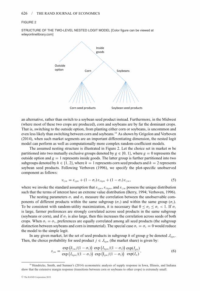
� GE crops (also known as transgenic crops) are the most visible agricultural manifestation ofmodern biotechnology and its use of recombinant DNA techniques. Their distinguishing featureis the insertion, in the plant’s genome, of one or more foreign genes that express desirable traits.In corn and soybeans, these traits have encompassed two sets of attributes: herbicide tolerance(HT) and insect resistance (IR). The vast majority of HT crops are tolerant to glyphosate, a broadspectrum herbicide marketed by Monsanto under the trademark Roundup R©. IR crops embed oneor more genes from the bacterium Bacillus thuringiensis (hence, the widely used “Bt” moniker),which emit proteins that are toxic to certain insects. For soybeans, the only trait with commercialrelevance thus far has been glyphosate tolerance (GT), whereas for corn, both GT and Bt traitshave been commercialized. Initially, GE varieties had a single trait, but over time, commercialvarieties have come to embed multiple GE traits, or what are often referred to as “stacked” GEtrait varieties. Figure 1 charts the diffusion pattern of GE varieties in US soybeans and corn,where “Bt maize” refers to varieties with at least one IR trait (alone or with the GT trait), and “GTmaize” refers to varieties with the GT trait (alone or in combination with other traits). Adoptionhas been rapid: GE corn and soybeans were first introduced in the United States in 1996 andwithin just 10 years, accounted for the majority of planted acres in both crops.
GE traits are valuable to farmers because they offer novel (cost-reducing and/or yield-enhancing) tools for weed and insect control. To guarantee adoption, however, GE traits need tobe combined with proven germplasm—the genetics accumulated from traditional breeding andselection activities that result in high-yielding and desirable commercial seed varieties. Thus, GEtraits and germplasm are truly complementary assets (Graff, Rausser, and Small, 2003), both ofwhich have become extremely valuable to seed manufacturers due to the increasing importance ofintellectual property rights (Moschini, 2010). Well before the advent of genetic engineering, the
C© The RAND Corporation 2019.

CILIBERTO, MOSCHINI AND PERRY / 619
TABLE 1 Market Shares in the US Corn and Soybean Seed Industry (percent), 2000–2015
2000–2003 2004–2007 2008–2011 2012–2015
CornMonsanto 11.2% 21.4% 34.0% 35.4%DuPont 36.0% 31.3% 31.5% 35.4%Syngenta 4.7% 10.3% 7.5% 5.7%Dow AgroSciences 5.2% 3.6% 4.1% 5.7%AgReliant 2.5% 4.8% 6.0% 6.8%Local and regional companies 40.5% 28.6% 16.9% 11.1%
SoybeansMonsanto 21.9% 23.4% 28.2% 27.6%DuPont 19.9% 24.9% 29.3% 33.3%Syngenta 3.4% 10.4% 10.5% 10.0%Dow AgroSciences 1.9% 1.6% 1.9% 4.8%AgReliant 1.1% 1.9% 1.8% 3.1%Local and regional companies 41.8% 36.0% 26.8% 18.6%Public/Saved seed 10.0% 1.8% 1.4% 2.7%
Note: The table reports market shares for the seed industry that emerged from the wave of market consolidation thatfollowed the introduction of GE traits. Source: Computed from GfK Kynetec data (2000–2011), and Farm JournalMagazine (2012–2015).
corn seed industry had already thrived through its use of hybridization (which requires farmers tobuy first-generation seeds for each planting) and trade secrets, which together effectively preventimitation. By contrast, commercial soybeans are self-pollinating and thus reproduce “true totype,” allowing farmers to replant seed from the previous season’s harvest without any loss inexpected yield. The introduction of patented GE traits, and the ability of seed companies to write(and enforce) restrictive retailing contracts forbidding farmers to save and replant seeds thatcontain such traits, thus significantly increased the profitability of selling soybean seeds.
The company Monsanto played a pioneering role in this process,1 and its commitmentto the development of GE crops has had major implications for the seed industry. The questto commercialize GE traits led to a wave of acquisitions and mergers that promoted a rapidconsolidation in the seed industry (Fernandez-Cornejo, 2004; Musselli Moretti, 2006). WhenMonsanto originally developed and patented its GE traits it did not have a presence in the seedindustry, and thus lacked direct access to commercial seed varieties. As a result, Monsanto pursuedtwo parallel strategies for the commercialization of its GE traits. First, it embarked on a seriesof acquisitions that, over time, transformed it into the largest seed company in the world. At thesame time, Monsanto aggressively licensed GE traits to other seed companies, which also spedup the availability of GE traits to farmers.
Monsanto’s critical acquisitions included Asgrow (in 1997), Dekalb (in 1998), and HoldenFoundation Seeds (in 1997). The early emphasis on broad “life science” companies also led toMonsanto becoming the agricultural subsidiary of Pharmacia Corporation in 2000, only to be spunoff as an independent company in 2002. Similar considerations led DuPont to acquire Pioneer, thedominant seed company at the time, in 1999. Syngenta was formed in 2000 as an agrochemicaland seed business from the consolidation and restructuring of major life science companies(Novartis and AstraZeneca). Dow AgroSciences, a subsidiary of Dow Chemical formed in 1997,acquired Mycogen in 1998. By the year 2000, when AgReliant (a joint venture of KWS andLimagrain) was also formed, the fundamental structure of the corn and soybean seed industry hadbeen established, although a number of other, smaller acquisitions would be made in subsequentyears (especially by Monsanto).
Market shares, reported as four-year averages for the 2000–2015 period, are displayed inTable 1. Data for 2000–2011 are from GfK Kynetec, the source of the proprietary data used in
1 Charles (2002) provides a fascinating account of the road to the commercial development and marketing of thefirst GE varieties.
C© The RAND Corporation 2019.

620 / THE RAND JOURNAL OF ECONOMICS
the econometric analysis. For the most recent years, the market shares reported in Table 1 arefrom the Farm Journal, a trade magazine.2 These market share data show an industry with twodominant firms (Monsanto and DuPont) who control approximately 60% of the soybean seedmarket and 70% of the corn seed market. Three other firms (Syngenta, Dow AgroSciences, andAgReliant) have considerably smaller but significant presence, with the industry completed by apanoply of local and regional companies. Table 1 also shows the almost complete disappearanceof the once-common practice of seed saving in soybeans (which accounted for more than 25% ofsoybean planting prior to the advent of GE varieties).
3. Data
� The data used in this study consists of a large set of farm-level observations of seed choicesby US corn and soybean farmers for the period 1996–2011. In particular, we use the soybean andcorn TraitTrak R© data sets, two proprietary data sets developed by GfK Kynetec, a unit of a majormarket research organization that specializes in the collection of agriculture-related survey data.GfK Kynetec constructs the TraitTrak R© data from annual surveys of randomly sampled farmersin the United States. The samples are developed to be representative at the crop reporting district(CRD) level.3 From 1996–2011, the data are based on responses from an average of 4716 farmersper year for maize and 3573 farmers per year for soybeans. In the survey, farmers are askedabout the types (brand and hybrid/variety identity), amounts, and cost of seed they purchase.4
Furthermore, with each purchase instance we observe the list of GE traits (if any) embedded inthe variety. Importantly, the period we observe covers the early stages of GE trait adoption up toits almost complete diffusion by 2011.
� Traits. Each of the various GE traits were introduced at different times in our sample.In soybeans, the GT trait was introduced by Monsanto in 1996 as Roundup Ready R© soybeans,and in corn, the GT trait was first commercialized in 1998. The main attraction of the GT traitis that, by allowing post-emergence applications of glyphosate without causing injury to thecrop, it greatly facilitates and reduces the cost of weed control.5 The first Bt trait in maize wasintroduced in 1996 and conferred resistance to the European corn borer (CB). Later Bt traits,which provided resistance to various species of corn rootworms (RW), were introduced in 2003.The attractiveness of Bt varieties is that they increase expected yields and reduce yield volatility(Fernandez-Cornejo et al., 2014; Xu et al., 2013), while also reducing the need for insecticides tocontrol pests. Unlike GT traits, which are highly complementary to a specific chemical, Bt traitssubstitute for chemical inputs (Perry et al., 2016).
2 The market share data reported by Farm Journal are based on polling industry analysts and executives, and havebeen published since 2009. In the three years (2009–2011) that the Farm Journal and GfK Kynetec data overlap, thefirm-level shares are very similar.
3 CRDs are multicounty substate regions identified by the National Agricultural Statistics Service of the USDepartment of Agriculture (USDA).
4 The Supplementary Information online web Appendix (Appendix B) provides a detailed description on the stepstaken to prepare the data.
5 The GT trait is not the only herbicide-tolerant trait in corn and soybeans. There is also a GE trait that providestolerance to the herbicide glufosinate. This trait was developed by Bayer and marketed under the tradename LibertyLink(LL). It has been available in some corn varieties since 1996 and in some soybean varieties since 2009. In our econometricanalysis, we ignore this trait for two reasons. First, it has been rarely adopted, especially in soybeans, where it only becameavailable in very limited quantities late in our sample. In corn, this trait can be found in more commercialized varieties,but this is mostly because it primarily served as a marker gene for the Bt traits (a marker gene is used to determine whetherthe insertion process was successful). Thus, most growers did not intend to use the LibertyLink trait when they purchasedvarieties that (incidentally) contained it. Indeed, based on pesticide data used in Perry et al. (2016), we found that only asmall fraction of corn producers who purchased seed containing the LL trait actually used any glufosinate herbicide. Thereare also traditionally bred varieties that are tolerant to the imidazoline herbicide (for corn) and to sulfonylurea herbicides(for soybeans). As with the LL trait, such varieties have had low adoption rates. Because our focus is on the differencein value between GE and non-GE crops, in our primary econometric analysis, we ignore these other herbicide-tolerancetraits.
C© The RAND Corporation 2019.

CILIBERTO, MOSCHINI AND PERRY / 621
TABLE 2 Adoption Rates for US Corn and Soybeans, Selected Years
Soybeans Corn Single Traits Corn Stacked Traits
Year GT GT CB RW GT-CB GT-RW CB-RW GT-CB-RW
1996 2.4% 0.7%1999 51.4% 2.5% 20.8% 0.0%2002 80.8% 7.2% 24.0% 2.2%2005 90.4% 15.8% 23.9% 1.2% 12.9% 1.2% 0.8% 1.0%2008 95.9% 19.2% 6.4% 0.1% 20.0% 0.8% 2.4% 36.6%2011 95.4% 19.2% 1.2% 0.0% 16.3% 0.5% 0.5% 53.3%
Note: This table reports detailed GE trait adoption rates (as percent of total planted acres for the corresponding crop).The Supplementary Information online web Appendix (Appendix C) reports data for all years in the 1996–2011 period.Source: Computed from GfK Kynetec data.
TABLE 3 Seed Prices for US Corn and Soybeans, Selected Years
Soybeans Corn Corn Single Traits Corn Stacked Traits
Year Non-GE GT Non-GE GT CB RW GT-CB GT-RW CB-RW GT-CB-RW
1996 17.20 21.27 24.60 30.451999 17.45 28.27 27.44 32.15 36.02 33.282002 17.41 26.84 28.63 32.40 36.96 37.36 45.022005 21.82 32.88 31.61 36.08 38.74 42.63 41.60 44.70 47.19 49.212008 26.21 36.37 41.92 53.73 49.85 60.69 58.39 61.99 62.27 69.262011 40.62 49.70 53.86 68.69 67.42 66.21 75.09 86.25 70.72 91.32
Note: This table reports data on average nominal seed prices paid by farmers ($/acre). The Supplementary Informationonline web Appendix (Appendix C) reports data for all years in the 1996–2011 period. Source: Computed from GfKKynetec data.
Figure 1 shows that the adoption of GE varieties, however fast by most standards,was gradual. This diffusion pattern is explained by both demand- and supply-side factors.On the demand side, learning and farmer heterogeneity played a role. On the supply side,the nature of the technology to develop and bring GE crops to market is critical. Becausethis plays an important role in our identification strategy, we provide more details at thatjuncture.
Table 2 reports detailed GE trait adoption rates (as a fraction of total planted acres forthe corresponding crop). Each column provides the annual adoption rate for a specific GE traitcombination (thus, in corn, the sum across columns is the total annual GE adoption rate). Amongall GE crop combinations, the most rapidly adopted were GT soybeans, which even surpassedthe rate at which corn hybrids were adopted (Griliches, 1957). By 2003, over 90% of land wasplanted to GT soybeans, and by 2011, it was 96%. The adoption of GT maize was slower, but stillachieved a 90% rate by 2011. The adoption of IR traits has been steady as well, with the CB traits(alone or in combination) attaining a 72% adoption rate, and RW traits (alone or in combination)achieving a 55% adoption rate by 2011. This table also illustrates the gradual penetration ofstacked-trait varieties. By 2011, the triple stack GT-CB-RW was adopted on 54% of maize acres.Note also that the RW trait, owing to its relatively late introduction, has had little diffusion asa stand-alone trait, instead becoming available to farmers primarily in combination with othertraits.
Table 3 reports nominal per-acre average seed costs for each GE trait combination. Theseprices reveal three important stylized facts about the seed markets. First, all prices have trendedup over time. Both GE and non-GE prices more than doubled from 1996 to 2011. Second, GEvarieties command a substantial premium over non-GE varieties. In soybeans, the premium was
C© The RAND Corporation 2019.
622 / THE RAND JOURNAL OF ECONOMICS
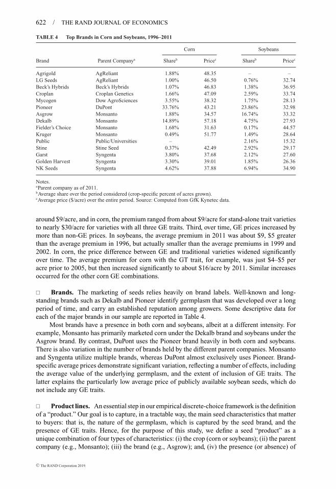
TABLE 4 Top Brands in Corn and Soybeans, 1996–2011
Corn Soybeans
Brand Parent Companya Shareb Pricec Shareb Pricec
Agrigold AgReliant 1.88% 48.35 – –LG Seeds AgReliant 1.00% 46.50 0.76% 32.74Beck’s Hybrids Beck’s Hybrids 1.07% 46.83 1.38% 36.95Croplan Croplan Genetics 1.66% 47.09 2.59% 33.74Mycogen Dow AgroSciences 3.55% 38.32 1.75% 28.13Pioneer DuPont 33.76% 43.21 23.86% 32.98Asgrow Monsanto 1.88% 34.57 16.74% 33.32Dekalb Monsanto 14.89% 57.18 4.75% 27.93Fielder’s Choice Monsanto 1.68% 31.63 0.17% 44.57Kruger Monsanto 0.49% 51.77 1.49% 28.64Public Public/Universities – 2.16% 15.32Stine Stine Seed 0.37% 42.49 2.92% 29.17Garst Syngenta 3.80% 37.68 2.12% 27.60Golden Harvest Syngenta 3.30% 39.01 1.85% 26.36NK Seeds Syngenta 4.62% 37.88 6.94% 34.90
Notes.aParent company as of 2011.bAverage share over the period considered (crop-specific percent of acres grown).cAverage price ($/acre) over the entire period. Source: Computed from GfK Kynetec data.
around $9/acre, and in corn, the premium ranged from about $9/acre for stand-alone trait varietiesto nearly $30/acre for varieties with all three GE traits. Third, over time, GE prices increased bymore than non-GE prices. In soybeans, the average premium in 2011 was about $9, $5 greaterthan the average premium in 1996, but actually smaller than the average premiums in 1999 and2002. In corn, the price difference between GE and traditional varieties widened significantlyover time. The average premium for corn with the GT trait, for example, was just $4–$5 peracre prior to 2005, but then increased significantly to about $16/acre by 2011. Similar increasesoccurred for the other corn GE combinations.
� Brands. The marketing of seeds relies heavily on brand labels. Well-known and long-standing brands such as Dekalb and Pioneer identify germplasm that was developed over a longperiod of time, and carry an established reputation among growers. Some descriptive data foreach of the major brands in our sample are reported in Table 4.
Most brands have a presence in both corn and soybeans, albeit at a different intensity. Forexample, Monsanto has primarily marketed corn under the Dekalb brand and soybeans under theAsgrow brand. By contrast, DuPont uses the Pioneer brand heavily in both corn and soybeans.There is also variation in the number of brands held by the different parent companies. Monsantoand Syngenta utilize multiple brands, whereas DuPont almost exclusively uses Pioneer. Brand-specific average prices demonstrate significant variation, reflecting a number of effects, includingthe average value of the underlying germplasm, and the extent of inclusion of GE traits. Thelatter explains the particularly low average price of publicly available soybean seeds, which donot include any GE traits.
� Product lines. An essential step in our empirical discrete-choice framework is the definitionof a “product.” Our goal is to capture, in a tractable way, the main seed characteristics that matterto buyers: that is, the nature of the germplasm, which is captured by the seed brand, and thepresence of GE traits. Hence, for the purpose of this study, we define a seed “product” as aunique combination of four types of characteristics: (i) the crop (corn or soybeans); (ii) the parentcompany (e.g., Monsanto); (iii) the brand (e.g., Asgrow); and, (iv) the presence (or absence) of
C© The RAND Corporation 2019.

CILIBERTO, MOSCHINI AND PERRY / 623
GE traits, specifically glyphosate tolerance (GT), corn borer (CB) resistance, and rootworm (RW)resistance.6
One of the important features to note about our product definition is that the number and typeof varieties that are aggregated within each product change over space and time. For example,from 2003 to 2011, the number of Pioneer corn varieties purchased with the GT trait rose from 9to 75. It is thus perhaps more appropriate to think of a “product” as a “product line,” one which issubject to change over time. One implication of this is that, within our econometric framework,the value of a GE product line should be permitted to change over time. As more and morehybrids are offered with a particular GE trait combination, a wider range of grower needs can bematched, raising the average value of that trait combination. Thus, in estimating our econometricmodel, we permit the return to GE varieties to differ over three subperiods. By doing so, wealso accommodate other largely exogenous changes in the industry, such as glyphosate going offpatent in 2000, and the commodity price boom of 2007–2008.
� Market definition. The definition of a market determines the set of available products toresiding farmers. We define a market as a CRD-year combination. As previously noted, CRDs aremulticounty, substate regions. We define a market at this level for three reasons. First, a CRD is thelevel at which the GfK Kynetec survey data are designed to be representative. Second, corn andsoybean varieties are bred to possess characteristics that suit particular agro-climatic conditions,and such conditions are relatively homogeneous within a given CRD. Finally, this is the spatialdefinition of markets that seed firms themselves use to analyze competitive issues (Monsanto,2009). Overall, this definitions results in 3874 markets (CRD-year combinations) encompassing294 distinct CRDs.7
A delicate issue, in this context, concerns the definition of the potential market size. Ideally,in a given market, this is given by the amount of land that could realistically be planted to corn orsoybeans. To identify this area, we use cropland measures from the Census of Agriculture (USDA-NASS, 2014). This is the main source of data concerning land use in the United States, and itis available at five-year intervals (Bigelow and Borchers, 2017). The cropland measure we useincludes “cropland used for crops” (itself encompassing three components: cropland harvested,crop failure, and cultivated summer fallow) and “idle cropland.” Perhaps unsurprisingly, weobserve very little variation in cropland acres over time. Hence, within each CRD, we assumethat the size of potential total seed demand is constant over our sample period, and specificallydefine it as the maximum of reported cropland across the four censuses that pertain to yearsencompassed by our sample period (1997, 2002, 2007, and 2012).8
Table 5 reports the average number of products in each market. For both corn and soybeans,the number of products increased steadily up until about 2007, and then declined thereafter. Thispattern reflects the fact that, as the adoption of GE traits increased (recall Figure 1), more andmore varieties became available to farmers both with and without GE traits. Later in the sample,as farmers’ demand for transgenic varieties exceeded that for traditionally bred varieties, someof the latter were discontinued. This pattern is more marked in corn, because there are three GEtraits (GT, CB, and RW), compared to one in soy (GT). The fact that the number of productschanged so significantly over time is a distinctive attribute of the industry. As we discuss in more
6 In principle, we could define a product at the individual hybrid/variety level. The number of available varieties inany given year, however, is too large to be of practical use. For example, 5065 distinct corn varieties and 2141 distinctsoybean varieties were purchased in 2007. By contrast, for that year, our definition results in 394 distinct products—small enough to be econometrically tractable, and large enough to still capture the fundamental elements of productdifferentiation in the seed industry.
7 There are 303 CRDs in the contiguous 48 states, but some are never present in the data because of negligible cornand soybean production. Also, some CRDs that are present are not sampled every year by GfK Kynetec. This occurs whenthe expected number of acres grown were too low to warrant the collection of data. On average, our data encompasses242 CRDs per year.
8 The Supplementary Information online web Appendix (Appendix B) provides further discussion on the definitionof the potential market size.
C© The RAND Corporation 2019.

624 / THE RAND JOURNAL OF ECONOMICS
TABLE 5 Average Number of Seed Products in a CRD, Selected Years
Year Total Corn Soybean Corn with GE Traits Soybeans with GE Traits
1996 10.8 6.5 4.3 0.3 0.41999 16.8 9.3 7.5 3.0 4.02002 18.0 11.1 6.9 5.3 4.92005 23.3 16.6 6.8 11.6 5.42008 27.9 21.7 6.2 18.1 5.62011 22.9 16.7 6.2 14.6 5.4
Note: A “seed product” is a unique combination of four types of characteristics—see Section 3 for more details. Thenumber of seed products in 1996 provide a good approximation on the number of products per market prior to theintroduction of GE traits. The Supplementary Information online web Appendix (Appendix C) reports data for all yearsin the 1996–2011 period. Source: Computed from GfK Kynetec data.
detail below, this has certain challenging implications for estimating the welfare associated withthe introduction of GE crops.
4. Farmers’ Seed Demand
� Each unit of observation in the data is a farmer’s choice of a seed product, denoted by j,to be planted on plot i of size Li . We model this decision as a discrete choice with a profit-maximization objective. The profit from planting plot i with seed product j can be expressed as�i j = RYi − W · Zi − Pj Si , where R is the output price, Yi is total output produced, Si is thequantity of seed, Zi is the vector of all inputs apart from seed and land (e.g., fertilizers, labor,energy, . . . ), W is the corresponding vector of input prices, and Pj is the price of seed productj. Note that we are omitting the rental price of land in this representation, so profit represents thereturn to the quasifixed input land.
The production function is written as Yi = Fj (Li , Si , Zi ). Note that this function, in principle,is specific to the identity of seed product j (this captures the fact that, compared with traditionalseed products, GE varieties may use different amounts and types of pesticides and/or a differentquantity of labor). We assume that this production function satisfies two basic properties: constantreturns to scale (i.e., doubling all inputs doubles total output); and, a fixed proportion of land andseed. That is, we can write the production function as
Fj (Li , Si , Zi ) = f j (Zi/Li ) × min{
Li , Si/λ j
}, (1)
where the parameter λ j denotes seed density (amount of seed per unit of land). By construction,f j (Zi/Li ) is strictly concave in the vector of input intensities Zi/Li . For a given plot of size Li ,and given that at an optimal solution we have Si = λ j Li , optimal input intensities Zi/Li implythat the per-acre maximized profit can be represented as �i j/Li = π j (R, W ) − λ j Pj , where theper-acre profit function π j (R, W ) is dual to the per-acre production function f j (Zi/Li ).
Because of the linear homogeneity property of π j (R, W ), the per-acre profit function is ho-mogeneous of degree one in the vector of all prices (R, W, Pj ). In the econometric application thatfollows, we pool seed choices across multiple years, during which prices changed dramatically.To account for this, we exploit the homogeneity property and deflate all prices by an appropriateinput price index WI and write per-acre profit in real terms, πi j ≡ �i j/(Li WI ), to obtain
πi j = π j (r, w) − pj , (2)
where πi j is the profit per acre on plot i when using seed product j , (r, w) is the vector of deflatedprices of output and all other inputs, and pj ≡ λ j Pj/WI is the deflated price of seed product j(expressed in per-acre terms).9
9 Specifically, for WI , we use the crop sector index for prices paid, published by the USDA. This index is normalizedto equal 1 in 2011, so that all profit and price data are interpreted in 2011 dollars.
C© The RAND Corporation 2019.

CILIBERTO, MOSCHINI AND PERRY / 625
� The econometric model. Building on equation (2), we model farmers as selecting theseed product that provides the highest expected profit per acre on plot i in market m, that is, theychoose product j such that
maxj
πi jm, j ∈ {0, 1, . . . , Jm} , (3)
where Jm denotes the number of seed products available in market m, and j = 0 denotes theoutside option.
We specify per-acre profits in (2) as being composed of an observable and unobservablepart. The observable part is assumed to be linear in parameters, and to depend on productcharacteristics, as well as a number of fixed and random effects. Specifically, the per-acre profitof choosing seed product j on plot i in market m is written as:
πi jm = x jγt[m] − pjm + ξc[ j],t[m] + ξc[ j],l[m] + ξc[ j],b[ j] + ξ jm + νi jm, (4)
or, following standard notation, πi jm = δ jm + νi jm , where δ jm denotes the mean profit thatis common across all plots within market m. Here, the vector x j comprises indicator variablesthat code for the presence of one or more GE traits in seed product j (these variables take valuezero for conventional seed products), and pjm is the associated price. Note that we allow theimpact of GE traits, via the coefficient γt[m], to possibly change over time (in the empirical resultsreported below, we specifically identify three distinct subperiods with different values associatedto GE traits). For the outside option, we follow standard convention and set πi0m = νi0m . Similar tomost empirical discrete-choice models, the price pjm enters linearly in equation (4). However, incontrast to consumer demand models, where linearity is typically a functional form simplification,in our context, it follows directly from the structural assumption of fixed proportions betweenland and seed, a property of the production technology that applies to this setting.
The terms ξc[ j],t[m], ξc[ j],l[m], and ξc[ j],b[ j] are, respectively, crop-time, crop-region, and crop-brand fixed effects. The subscript notation follows Gelman and Hill (2007): c[ j] indicates thecrop output associated with seed product j (either soybeans or corn), b[ j] indicates the brand ofseed product j (for example, Dekalb), t[m] denotes the year corresponding to market m, and l[m]denotes the CRD corresponding to market m (l stands for location). This large set of fixed effectscontrols for unobservable heterogeneity in yields, output, and input prices across time, regions,brands, and crops. The term ξ jm captures the unobserved product-market-specific componentsthat motivate our identification discussion below. Finally, νi jm is the unobserved plot-specificcomponent.
To make the choice model in (3)–(4) operational, we need distributional assumptions onthe plot-specific unobservable νi jm . We model the demand for corn and soybean seed productsusing a two-level nested logit specification (Verboven 1996; Bjornerstedt and Verboven, 2016).We specify the upper level as consisting of the outside option and the set of inside options, wherethe latter consists of all corn and soybean seed products. We then further partition the insideoptions into two subgroups, one for soybean seed products and the other for corn seed products.
Partitioning the choice problem in this way is consistent with basic facts about US cornand soybean production. Less than 5% of corn and soybean production occurs on farms with asingle crop (MacDonald, Korb, and Hoppe, 2013). Farms that produce both corn and soybeansare ubiquitous, especially in the Midwest. Because planting and harvest timings differ somewhatbetween these two crops, economies of scope can be obtained in the use of farm labor andmachinery. Crop diversification on the farm can also be motivated by rotation considerations(Hennessy, 2006). Indeed, the practice of alternating between corn and soybeans on a givenplot is widespread in US agriculture, as it has been shown to increase profit by increasing yields,reducing fertilizer needs, and improving weed control (Bullock, 1992). Hence, a given plot plantedto corn (soybeans) in year t − 1 is much more likely to be planted to soybean (corn) in year t . Thus,our presumption is that, for example, if the expected return to a corn seed product on a given plot isunattractive, a grower will typically be much more likely to consider another corn seed product as
C© The RAND Corporation 2019.
626 / THE RAND JOURNAL OF ECONOMICS
FIGURE 2
STRUCTURE OF THE TWO-LEVEL NESTED LOGIT MODEL [Color figure can be viewed atwileyonlinelibrary.com]
Outsideop�on
Insidegoods
Corn Soybeans
Corn seed products Soybean seed products
an alternative, rather than switch to a soybean seed product instead. Furthermore, in the Midwest(where most of these two crops are produced), corn and soybeans are by far the dominant crops.That is, switching to the outside option, from planting either corn or soybeans, is uncommon andeven less likely than switching between corn and soybeans.10 As shown by Grigolon and Verboven(2014), when such market segments are an important differentiating dimension, the nested logitmodel can perform as well as computationally more complex random-coefficient models.
The assumed nesting structure is illustrated in Figure 2. Let the choice set in market m bepartitioned into two mutually exclusive groups denoted by g ∈ {0, 1}, where g = 0 represents theoutside option and g = 1 represents inside goods. The latter group is further partitioned into twosubgroups denoted by h ∈ {1, 2}, where h = 1 represents corn seed products and h = 2 representssoybean seed products. Following Verboven (1996), we specify the plot-specific unobservedcomponent as follows:
νi jm = εigm + (1 − σ2) εihgm + (1 − σ1) εi jm, (5)
where we invoke the standard assumption that εigm , εihgm , and εi jm possess the unique distributionsuch that the terms of interest have an extreme value distribution (Berry, 1994; Verboven, 1996).
The nesting parameters σ1 and σ2 measure the correlation between the unobservable com-ponents of different products within the same subgroup (σ1) and within the same group (σ2).To be consistent with random-utility maximization, it is necessary that 0 ≤ σ2 ≤ σ1 < 1. If σ1
is large, farmer preferences are strongly correlated across seed products in the same subgroup(soybeans or corn), and if σ2 is also large, then this increases the correlation across seeds of bothcrops. When σ2 = σ1, preferences are equally correlated among all seed products (the subgroupdistinction between soybeans and corn is immaterial). The special case σ1 = σ2 = 0 would reducethe model to the simple logit.
In any given market, let the set of seed products in subgroup h of group g be denoted Jhgm .Then, the choice probability for seed product j ∈ Jhgm (the market share) is given by:
s jm = exp(δ jm/(1 − σ1)
)
exp(Ihgm/(1 − σ1)
) exp(Ihgm/(1 − σ2)
)
exp(Igm/(1 − σ2)
) exp(Igm)
exp(Im), (6)
10 Hendricks, Smith, and Sumner’s (2014) econometric analysis of supply response in Iowa, Illinois, and Indianashow that the extensive margin response (transitions between corn or soybeans to other crops) is extremely small.
C© The RAND Corporation 2019.

CILIBERTO, MOSCHINI AND PERRY / 627
where Ihgm , Igm , and Im are “inclusive values” defined as follows (Bjornerstedt and Verboven,2016):
Ihgm = (1 − σ1) ln∑
k∈Jhgm
exp (δkm/(1 − σ1)) (7)
Igm = (1 − σ2) ln∑
h∈{1,2}exp
(Ihgm/(1 − σ2)
)(8)
Im = ln(1 + exp(Igm)
). (9)
Again, in our setting, g = 1 denotes the group of all inside goods, and this group comprisestwo subgroups (h = 1, 2). Based on this specification, recalling the definition of δ jm , we obtainthe estimating equation for our two-level nested logit:
ln(s jm/s0m) = x jβt[m] − α pjm + σ1 ln(s jm/Sh1m)
+ σ2 ln(Sh1m/S1m) + ξc[ j],t[m] + ξc[ j],l[m] + ξc[ j],b[ j] + ξ jm, (10)
where Sh1m ≡ ∑j∈Jh1m
s jm is the aggregate share of all products in subgroup h ∈ {1, 2}, andS1m = S11m + S21m is the total share of all inside goods. Hence, s jm/Sh1m is the (conditional) shareof seed product j within subgroup h (i.e., corn or soybean), and Sh1m/S1m is the (conditional) shareof subgroup h in group g = 1 (the group of all inside goods). Finally, s0m = 1 − S1m is the shareof the outside option.
As we discuss further below, these shares are endogenous and therefore require instruments.In addition, the coefficient that we estimate on the price variable, α ≡ 1/μ, is the reciprocal ofthe scale parameter μ associated with the i.i.d. extreme value error term. This parameter canbe interpreted as a measure of preference heterogeneity in the population (Anderson, De Palma,and Thisse, 1992). Also, the parameters β in equation (10) are related to γ in equation (4) byγ = β/α.
� Identification. The key identification issue is the endogeneity of seed prices, which seedmanufacturers set taking into account the fact that they are competing in an oligopoly, andfactoring in differentiation across products. The solution to this problem, which was first proposedby Bresnahan (1987), and later adopted, among others, by Berry (1994) and Berry, Levinsohn,and Pakes (1995), consists of assuming that the location of firms’ varieties in the product spaceis exogenous, and this source of exogenous variation across time and geographical markets canbe exploited to identify the parameters of the econometric model.
This assumption seems particularly reasonable in the seed industry, because individual firmshave shown a clear willingness to introduce traits into their seed lines as soon as they becomeavailable. Furthermore, in this context, it is crucial to appreciate that the technology to bring GEseeds to market entails a lengthy and complex process (Mumm and Walters, 2001). Molecularbiology and tissue culture techniques are used to introduce the gene(s) of interest into plantcells. Such transformed cells are then regenerated into whole plants, each of which is a distincttransformation “event” (which thus embeds the particular genotype, often not of commercialinterest itself, used at the transformation stage). Extensive molecular and agronomic testingselects the best among the many events that are generated. The next step is the integration ofthe selected event into elite germplasm. For each commercial variety eventually developed, thisrequires repeated iteration of backcross breeding (crossing to a recurrent parent) to achieve thedesired germplasm purity.11 A key role is also played by the GE regulatory structure adopted bythe United States, where the unit of evaluation is a unique event (McHughen and Smyth, 2008).
11 An alternative to backcrossing is forward breeding, which has some disadvantages in maize but may be preferablefor crops (such as soybeans) for which cross-pollination is difficult.
C© The RAND Corporation 2019.

628 / THE RAND JOURNAL OF ECONOMICS
The process of clearing the regulatory hurdles is onerous and, although it can be run concurrentlywith trait integration, is itself rather lengthy (Bradford et al., 2005).
The entire process of producing GE varieties is very long: even abstracting from genediscovery and the transformation phase, the average time for trait integration into elite germplasm,field testing, regulatory compliance, and seed bulk-up needed to launch a commercial productis about seven years (Prado et al., 2014). Moreover, this process is complex, and the need forextensive testing introduces randomness at various junctures. Even at the last stage of field testing,the seed firm’s “ . . . supply management may be dealing with a number of events or candidateproducts that ultimately will not proceed to commercialization.” (Mumm and Walters, 2001).Seed companies also invest in traditional breeding activities to improve germplasm, but again,they have an incentive to commercialize their best products at any given point in time. Moreover,the turnover of commercialized varieties is fairly high, with varieties exiting a market sometimesafter only two or three years (Magnier, Kalaitzandonakes, and Miller, 2010). Overall, this suggeststhat the introduction of new products is predetermined, embeds stochastic elements, and is largelyexogenous to pricing decisions.
Following Berry, Levinsohn and Pakes (1995) we use functions of the traits in competingvarieties as our instruments. As GE traits are the main characteristics that vary over seed varieties,this amounts to counting up the unique number of competing GE seed products. Specifically, wecompute the total number of competing products (irrespective of GE traits) by: market; marketand brand; market and parent company; market and crop; market, brand, and crop; and market,parent company, and crop. This results in six instrumental variables. We then compute the samevariables for each of the three GE traits, plus non-GE products: GT, CB, RW, and non-GE. Thisresults in an additional 24 instrumental variables (in total, there are 30 instrumental variables).
5. Results
� Table 6 presents the estimation results for four different specifications of the seed demandmodel, which differ by the number of fixed effects that control for unobserved heterogeneity andby the type of logit model (simple logit versus nested logit). Specifically, columns 1 and 2 containresults for the two-level nested specification discussed in Section 4, and columns 3 and 4 containresults for the simple logit specification, which is equivalent to the special case σ1 = σ2 = 0.Our primary goal with this table is to establish how these modelling differences, and the use ofinstrumental variables, affect the estimated coefficients and the implied elasticities.
In all four specifications in Table 6, the coefficients are estimated fairly tightly, and thepricing and nested logit terms have the expected signs and ordering. The specification in column1 is estimated with the richest set of fixed effects, which include year, CRD, and brand fixedeffects, each of which are also interacted with the crop dummy variable (permitting responseto differ between corn and soybeans). The year fixed effects control for temporal industry-widechanges, such as changes in output (corn and soybeans) prices, or changes in the prices ofnonseed production inputs (e.g., fuel). The CRD fixed effects control for unobserved, time-invariant regional-specific effects, such as the length of the growing season, soil quality, andweed pressure. The brand fixed effects control for unobserved (perceived and real) differences inthe returns to each of the various brands. For example, in a given region, Pioneer seeds may begenerally regarded by growers as high-yielding, and because of this, their prices may be higher.As it concerns fixed effects, the difference between column 1 and columns 2–4 is that the fixedeffects in the latter are not interacted with a crop dummy variable.
Column 1 of Table 6 contains the most general specification of this table. The price coeffi-cient is statistically significant and negative, as expected, and the nesting parameters are tightlyestimated, with an ordering that is consistent with profit maximization (0 < σ2 < σ1 < 1). Theirmagnitude indicates strong correlation within nests, suggesting that once producers decide onwhich crop to plant on a given plot, they are unlikely to switch, both to another crop (corn orsoybeans), and even less so to something besides corn or soybeans. This finding supports the
C© The RAND Corporation 2019.

CILIBERTO, MOSCHINI AND PERRY / 629
TABLE 6 Estimated Parameters of Seed Demand Models
Nested Logit Basic Logit
(1) (2) (3) (4)
Price −0.0212 −0.0155 −0.0504 −0.0049(0.0020) (0.0012) (0.0028) (0.0005)
σ1 0.8493 0.8123(0.0083) (0.0084)
σ2 0.3978 0.6207(0.0558) (0.0184)
Soy GT trait 0.4070 0.3572 1.4309 0.8182(0.0319) (0.0213) (0.0431) (0.0214)
Corn GT trait 0.1962 0.1296 0.3410 −0.1380(0.0204) (0.0132) (0.0328) (0.0149)
Corn RW trait 0.2053 0.1515 0.5177 0.0229(0.0219) (0.0150) (0.0357) (0.0189)
Corn CB trait 0.1642 0.1124 0.2770 −0.1179(0.0172) (0.0112) (0.0279) (0.0140)
Soy dummy −0.2395 −0.6811 −0.0294(0.0200) (0.0447) (0.0206)
Elasticities:Own −6.990 −4.133 −2.637 −0.254Cross: within crop 0.481 0.244 0.045 0.004Cross: across crop 0.053 0.075 0.045 0.004Cross: outside good 0.019 0.014 0.045 0.004IVs? Yes Yes Yes NoFixed effects Crop × Year,
Crop × Brand,Crop × CRD
Year, CRD, Brand Year, CRD, Brand Year, CRD, Brand
Note: This table presents the estimation results for four different specifications of the seed demand model. Standard errorsare reported in parentheses. N = 79,260.
rationalization of the two-level nested logit specification provided earlier. The remaining estimatespresented in column 1 are for the coefficients associated with the GE trait dummy variables. Inall cases, the estimates are positive, indicating that farmers are willing to pay a positive amountfor each trait. These coefficients provide the basis for estimating farmers’ willingness- to- pay(WTP) for the innovation of GE traits, which we consider extensively in Section 6.
Column 2 in Table 6 includes fewer controls by postulating year, CRD, and brand fixed effectsthat are not crop-specific. Relative to column 1, the results remain mostly unchanged, however,the subgroup nesting parameter, σ2, increases in size and the price coefficient is significantlysmaller. This likely reflects the fact that including crop-specific effects controls for crop-specificunobservable differences in products that are correlated with prices. In moving from column 2 tocolumn 3, we move from the two-level nested logit model to the basic logit model. This reducesflexibility in the substitution pattern between seed products (and also means that the coefficientsof the price variable are not directly comparable). Finally, column 4 presents results for the simplelogit model without instrumental variables for prices. The price coefficient without instrumentsis substantially smaller (in absolute value) than in column 3. The fact that the price coefficientincreases so significantly when going from column 4 to column 3 indicates that prices are indeedendogenous, a finding that is typical of differentiated product markets (Berry, Levinsohn, andPakes, 1995; Trajtenberg, 1989).
� Elasticities. To better convey the implications of the different coefficients, Table 6 alsoreports mean own- and cross-price elasticities. Elasticity formulae for our two-level nested logitmodel are derived based on Bjornerstedt and Verboven (2016). The coefficients of the model incolumn 1 imply a mean own-price elasticity equal to −6.99, which is quite elastic. The estimated
C© The RAND Corporation 2019.

630 / THE RAND JOURNAL OF ECONOMICS
TABLE 7 Nested Logit Model: Subadditivity and Time Variation of Trait Effects
(1) (2)
Price −0.0182 (0.0023) −0.0182 (0.0023)σ1 0.8642 (0.0079) 0.8176 (0.0096)σ2 0.4428 (0.0541) 0.3718 (0.0567)Soy GT trait 0.3549 (0.0341)Corn GT trait 0.1925 (0.0278)Corn RW trait 0.2062 (0.0306)Corn CB trait 0.1693 (0.0250)Multiple traits −0.0687 (0.0172)Soy GT trait, 1996–2000 0.3075 (0.0383)Soy GT trait, 2001–2006 0.4366 (0.0373)Soy GT trait, 2007–2011 0.4681 (0.0368)Corn GT trait, 1996–2000 0.0251 (0.0387)Corn GT trait, 2001–2006 0.0651 (0.0264)Corn GT trait, 2007–2011 0.3100 (0.0328)Corn CB trait, 1996–2000 0.0952 (0.0340)Corn CB trait, 2001–2006 0.1036 (0.0262)Corn CB trait, 2007–2011 0.2276 (0.0260)Corn RW trait, 2001–2006 0.0169 (0.0402)Corn RW trait, 2007–2011 0.2417 (0.0293)Multiple traits, 1996–2000 −0.0314 (0.0944)Multiple traits, 2001–2006 −0.0187 (0.0220)Multiple traits, 2007–2011 −0.1360 (0.0202)
Note: This table presents the estimation results for two different specifications of the seed demand model. Both modelsinclude the same fixed effects as model (1) in Table 6, as well as IVs. Standard errors are reported in parentheses. N =79,260.
own-price elasticities get progressively smaller (in absolute value) in columns 2–4, as we includefewer controls and less flexibility in the substitution patterns. For the basic logit model in column4, the implied mean own-price elasticity is just −0.25, an inelastic response which is inconsistentwith models of profit-maximizing seed firms that sell differentiated products. For the most generalmodel of column 1, the mean cross-price elasticities are 0.48 within a crop (e.g., from a soybeanseed product to another soybean seed product) and 0.05 across crops (e.g., from a soybean seedproduct to a corn seed product). The difference between these mean elasticities underscores therelevance of the assumed nesting structure: growers more readily substitute toward products ofthe same crop in response to price increases in any given seed product. The estimated cross-priceelasticity for the outside good is very small at just 0.02, or about one fortieth the magnitude ofthe mean cross-price elasticity for products of the same crop. This indicates that the aggregatedemand for corn and soybean seed products is rather inelastic.
� Subadditivity and time-varying GE trait effects. Table 7 provides results for two ad-ditional, more general parameterizations of the nested logit model. The model in column (1)allows for complementarities (or rivalries) among GE traits as inputs. More specifically, thereis an additional indicator variable, Multiple Traits, that takes a value of one whenever there ismore than one GE trait in a seed product.12 The negative and significant coefficient in Table 7 forMultiple Traits indicates subadditivity in the value of products with multiple GE traits. That is,on average, farmers are willing to pay a bit less for each of multiple GE traits compared to whatthey would pay for those traits in isolation. This result is related to, but distinct from, that of Shi,Chavas, and Stiegert (2010), who find subadditivity in the pricing of stacked GE trait varieties.
12 We also estimated regressions with stacked variables for all of the possible GE trait combinations: GT-CB,GT-RW, CB-GT, and GT-CB-RW. We use a generic stacked variable for its parsimony and because certain stacks are veryseldom observed. Nonetheless, the results are largely unchanged in these alternative formulations.
C© The RAND Corporation 2019.

CILIBERTO, MOSCHINI AND PERRY / 631
Our result, being rooted in a structural demand model, relates specifically to the value farmersplace on GE traits.
Column (2) of Table 7 contains the estimates that we use for the welfare analysis. Thisrepresentation permits the return to the various GE traits to differ across three subperiods. Asnoted earlier, this allows for the possibility that the average return to GE traits vary in accordancewith the range of germplasm that incorporates them, and it is also consistent with importantevents that likely affected the return to GE products: the expiration of Monsanto’s glyphosatepatent in 2000; and, the sharp increase in crop output prices in 2007 as part of the most recentmajor commodity price boom (Baffes and Haniotis, 2010; Wright, 2011). The results in column2 strongly indicate that the returns to GE varieties were indeed different and increasing overthese three subperiods. Specifically, the coefficient on the Soy GT Trait increased from 0.3075in 1996–2000 to 0.4681 in 2007–2011, and the coefficient on the Corn GT Trait increased from0.0251 in 1996–2000 to 0.3100 in 2007–2011. The Multiple Traits coefficient also changes overtime, becoming more negative in the final subperiod.
6. Welfare
� The development and commercialization of GE crops has represented a major technologicalinnovation for agriculture. The estimated seed demand model presented in the foregoing providesthe ideal framework for a novel empirical assessment of the welfare effects of this innovation. Toreach robust conclusions, we adopt a two-pronged approach. First, we use the estimated demandmodel to compute farmers’ WTP for GE traits. This willingness-to-pay a premium for GE traits isequivalent to an upward shift in the demand facing seed companies. Hence, the ability to bundleGE traits with traditional germplasm holds the potential for seed companies to increase pricesand boost revenues. Together with observed planted acres and price premia for GE products,estimated WTPs permits a first look at the total surplus created by GE varieties, as well as itsdistribution between farmers and seed firms. Alternatively, we use the structure of the estimateddemand model to estimate the total net value of GE traits to farmers (increase in expected profit)by simulating a counterfactual in which GE traits are not available. This simulation requiresknowledge of what conventional seed prices would have been in the absence of GE products.To compute such prices, we follow Hausman and Leonard (2002) by using a reduced-formhedonic price equation. By making assumptions on the nature of the unobservables, we estimatecounterfactual prices (and counterfactual choice sets) had GE varieties not been introduced. Theresults of both of these approaches to welfare calculations are presented below.
� Farmers’ willingness-to-pay for GE traits. The WTP for a given GE trait combinationis the maximum amount ($/acre) that a farmer would be willing to part with in order to havethat particular combination added to a seed product line. To calculate farmers’ WTP for GEtraits, we use the demand estimates from the most general model (column 2 of Table 7). In atypical discrete-choice random-utility framework (e.g., the logit model), the (marginal) WTP fora particular characteristic is given by the ratio of the estimated coefficient on that characteristic tothe estimated coefficient on the price variable (Train, 2009). Although our latent return functionis cardinal and denominated in dollars per acre (rather than utility), the general procedure remainsthe same: the WTP for a particular GE trait is the ratio of the coefficient associated with that traitand the estimated price coefficient. As noted earlier, the estimated price coefficient is the reciprocalof the scale parameter of the extreme value distribution. Thus, in dividing by the price coefficient,we are simply removing the scale factor from the trait coefficients. For example, the WTP for theGT trait in soybeans is: βSoyGT /α. For a combination of GE traits, the relevant WTP is recoveredby dividing the sum of the associated trait coefficients by the price coefficient. For example, theWTP for the stacked combination GT-CB-RW in corn is (βCornGT + βC B + βRW + βMultiple)/α.
Table 8 contains WTP estimates for each of the GE trait combinations in each of the varioussubperiods. Because all prices in the analysis are deflated by an input price index normalized
C© The RAND Corporation 2019.

632 / THE RAND JOURNAL OF ECONOMICS
TABLE 8 Willingness-to-Pay for GE Products (2011 $/acre)
Trait(s) 1996–2000 2001–2006 2007–2011
Soy GT 16.88 23.96 25.69(0.76) (1.58) (2.23)
Corn GT 1.38 3.57 17.01(2.01) (1.06) (0.75)
Corn CB 5.22 5.69 12.49(1.33) (0.84) (0.81)
Corn RW 0.93 13.26(2.11) (0.66)
Corn GT-CB 4.88 8.23 22.04(5.1) (1.13) (0.82)
Corn GT-RW 3.47 22.81(2.34) (0.77)
Corn CB-RW 5.58 18.29(2.11) (0.56)
Corn GT-CB-RW 9.16 35.30(2.97) (0.99)
Note: This table contains WTP estimates for each of the GE trait combinations, in each of the three subperiods. Theseestimates are based on the most general estimated model (Column 2 of Table 7). Standard errors are reported in parentheses.
to equal 1 in 2011, all estimates are in real terms (2011 dollars). All of the estimates appearreasonable and are in line with what might be expected, given knowledge of seed prices and theobserved adoption patterns by farmers. The WTP for the GT trait in soybeans was $16.88 peracre in the first subperiod, rose to $23.96/acre in the 2001–2006 subperiod, and then rose slightlyagain to $25.69/acre in the 2007–2011 subperiod. The WTP for the corn GT trait also increasedover time, but followed a different pattern. From 1996–2000, the WTP for GT corn was only$1.38/acre. It then grew to $3.57/acre from 2001–2006, and then increased substantially to $17.01from 2007–2011. A similar pattern occurred for the other corn GE traits (CB and RW). For thestand-alone and stacked combinations, the increase in value was greatest from the second to thethird subperiod. The increase in the value of the triple-stack GT-CB-RW was particularly large,from $9.16 in the second subperiod to $35.30 in the last subperiod.
The standard errors reported in Table 8 suggest that, overall, the WTPs for the GT trait insoybeans and for the CB trait in corn are precisely estimated. WTPs for the GT trait in corn aretightly estimated for the last two subperiods, and the WTPs for RW corn are only precise in thefinal subperiod. This is consistent with the adoption patterns illustrated in Table 2; the initiallyslower adoption of some corn GE traits translates into larger standard errors.
A common finding among all trait combinations is that their value increased over time, whichis consistent with the temporal increase in the observed shares for GE products. One contributingfactor has been falling glyphosate prices. Subsequent to the expiration of Monsanto’s mainglyphosate patent in 2000, the price of glyphosate fell from $12.42/lb. in 2000 to $4.74/lb. in2011 (note: a standard application is 0.75 lb./acre). Because glyphosate is used more heavilywith GT crops, a lower price for this herbicide reduces the farmers’ production cost of GTcrops relative to non-GT crops, reinforcing their adoption incentive. A second factor is risingoutput prices in the latter years of our sample. The average price received by farmers for corn, asreported by the United States Department of Agriculture (USDA), increased from $2.22/bu. inthe subperiod 2001–2006 to $4.35/bu. in the final subperiod 2007–2011, whereas for soybeans,the corresponding price change was from $6.03/bu. to $10.30/bu. Naturally, an increase in theoutput price increases the value of yield-enhancing inputs. As noted, previous work has shownthat IR traits in corn increase yields (Nolan and Santos, 2012; Xu et al., 2013), and thus, higheroutput prices increase the relative value of the CB and RW traits. A third factor is learning, whichmay have played a role earlier on. Although the limited availability and breadth of GE seeds was
C© The RAND Corporation 2019.

CILIBERTO, MOSCHINI AND PERRY / 633
TABLE 9 Total Surplus and Its Imputed Distribution from GE Innovation ($ million)
Period Crop Total Surplus Firm Revenues Imputed Farmers’ Net Returns
1996–2011 Soybeans 19,424 11,132 8,292Corn 11,233 13,206 −1,973Total 30,657 24,338 6,319
1996–2000 Soybeans 1,906 1,940 −34Corn 265 792 −527Total 2,171 2,733 −562
2001–2006 Soybeans 8,731 5,086 3,645Corn 1,122 2,531 −1,409Total 9,853 7,617 2,236
2007–2011 Soybeans 8,787 4,105 4,682Corn 9,846 9,883 −37Total 18,633 13,989 4,644
Note: Total surplus figures in column 3 of this table are obtained by multiplying the WTP estimates (as reported inTable 8) by the observed planted acres of each GE variety. The estimated seed industry revenues attributable to GE traitsin column 4 are obtained by multiplying the average price premia (as reported in Table 3 for selected years, but deflatedby the crop sector input price index used in estimation) with observed planted acres of GE crops. Imputed net returns tofarmers due to GE traits, reported in the last column, are the difference between columns 3 and 4.
another factor affecting adoption in the first few years, anecdotally it seems that most producersalso had an initial trial run with GE crops before wholly committing to this technology. In otherwords, our WTP methodology is rooted in producers’ perceived value of GE traits, which likelyincreased as evidence of the efficiency-enhancing properties of GE traits accumulated.
A final element to keep in mind in interpreting the results relates to our approach to productdefinition. Recall that we define a product as a crop-brand-trait combination, which means thatwe aggregate over varieties within each combination. Over time, the types and number of thesevarieties changed within each defined product. As noted earlier, for example, the number ofPioneer corn hybrids offered with the GT trait (across all markets) was 9 in 2003 and 75 in 2011.Thus, the various GE trait coefficients also capture the range of varieties that were offered withina particular product line. The wider the range of seeds offered within a product line, the morediverse the set of needs the line could match. For example, it is likely that the 9 corn GT hybridsoffered by Pioneer in 2003 were not as ideally matched to farmer’s needs as the 75 corn GThybrids that the same company offered in 2011, and thus, the average 2003 value of the PioneerGT line across all farmers was correspondingly smaller.
� Total incremental surplus and seed revenues from GE traits. WTP estimates permita first look at the welfare benefits that accrued to farmers and seed manufacturers from theintroduction of GE traits. Specifically, multiplying the WTP estimates (as reported in Table 8) bythe observed planted acres of each GE trait provides a first-order approximation to the total surpluscreated by the innovation. We can also use the average price premia from Table 3 (deflated by thecrop input price index) along with observed planted acres of GE crops to compute an estimate ofthe seed industry revenues attributable to GE traits. The accuracy of these procedures rests on theassumptions that the number of acres cultivated to corn and soybeans would have been the samehad GE traits not been introduced, and that observed conventional seed prices would have beenthe same absent the GE innovation. The results are reported in Table 9.
Over the entire period 1996–2011, total surplus is estimated at $30.7 billion (in 2001dollars)—$19.4 billion for soybeans and $11.2 billion for corn. During the same period, we findthat the availability of GE traits increased seed industry revenues by $24.3 billion—$13.2 billionin corn seeds and $11.1 billion in soybean seeds. Finally, the values in the last column of Table 9report the net returns to farmers, imputed as the difference between total surplus and seed industryrevenues, associated with the adoption of GE traits. Over the entire period 1996–2011, we find
C© The RAND Corporation 2019.

634 / THE RAND JOURNAL OF ECONOMICS
that farmers’ net returns were $6.3 billion higher because of the introduction of GE traits. Overall,these results suggest that seed manufacturers appropriated the larger portion of the surplus createdby GE traits.
Imputed net returns to farmers show a clear difference between soybeans and corn. Perhapssurprisingly, the calculations reported in Table 9 suggest that net returns to corn farmers havebeen negative (a total loss of nearly $2 billion, most of which occurred in the first two subperiodsof the analysis). To put this result in context, recall that the model’s parameterization assumes that(within a given subperiod) all farmers have the same WTP parameters vis-a-vis GE traits. Insofaras the value of GE traits was heterogeneous across farmers, our WTP estimates, which reflect anaverage value across all farmers, underrepresent the value of GE traits to actual adopters. Also,as noted, the WTP estimates for GE corn traits are imprecise in the first two subperiods, whichmake the corresponding total surplus estimates less reliable. Moreover, whereas the procedureunderlying Table 9 is attractive because it uses observed data and does not make additionalassumptions on the structure of the unobservables, a major weakness is that it maintains thatprices and quantities would have been the same had GE seeds not been introduced. This isan undesirable assumption for several reasons. First, the introduction of GE seeds resulted inmore seed products available to farmers, especially in corn. This increased differentiation meantthat farmers could choose seed products that better matched their growing conditions.13 Second,standard considerations suggest that conventional seed prices would have been higher in theabsence of GE traits. Similarly, if GE traits were indeed valuable, then total corn and soybeanacres would have been lower in the absence of GE traits. Finally, observed average price premiafail to account for spatial price heterogeneity.
These limitations can be addressed by computing counterfactual prices that account for anycompetitive price effects that GE varieties may have exerted on non-GE products, by using thestructure of the estimated demand model to compute counterfactual conventional seed productsshares, and by developing counterfactual scenarios that can account for the impact of GE-inducedproduct differentiation on farmers’ expected profits and seed industry revenues.
� Counterfactual prices. To address the question of what (conventional) seed prices wouldhave been without the GE technology, a possible approach is to construct a full structural equi-librium model embedding the main drivers of price changes in the industry. With this method,the literature generally maintains that firms behave as Bertrand oligopolists with differentiatedproducts, and then simulates counterfactual solutions under alternative assumptions (Nevo, 2001;Petrin, 2002; Goeree, 2008). The upside of this approach is that it makes the assumed economiccontext fully transparent. Such a structural model presents challenges in our context, however.This is because, although seed firms own their own germplasm, most of them have engagedin extensive licensing (and cross-licensing) arrangements for GE traits. Hence, the standardBertrand-Nash price equilibrium conditions for differentiated products are not appropriate forthis setting. Furthermore, the terms of the GE trait licensing arrangements between firms are notin the public domain (Moss, 2010), which makes it problematic to develop a suitable structuralrepresentation of the supply side, an undertaking we leave for future research.
To proceed, we use a reduced-form hedonic approach, as in Hausman and Leonard (2002).Although this method permits us to avoid specifying an explicit structural equilibrium model,and thus eschew the thorny issue of what to do about GE trait licensing, the validity of thisapproach rests on some strong conditions. In general, the reduced-form procedure is valid if GEtrait entry were exogenous across markets and time, which would exclude the possibility that
13 The proliferation of corn varieties documented in Table 5 reflects the fact that, upon the introduction of GEvarieties, the same germplasm was often available to farmers both with and without GE traits. Farmers with plotsexposed to higher pest pressure would have a higher propensity to adopt the GE variety, whereas farmers with lower pestpressure may find a better match with the corresponding conventional variety. This effect is arguably more importantfor IR traits in corn because “insect infestation varies much more widely across locations than does weed infestation”(Fernandez-Cornejo and Caswell, 2006).
C© The RAND Corporation 2019.

CILIBERTO, MOSCHINI AND PERRY / 635
entry responds to market demand or cost shocks. This condition is unlikely to hold strictly in anyempirical context. Still, our setting and approach display features that make this assumption moretenable. As discussed extensively earlier, the technology of introducing GE traits into commercialgermplasm takes several years, it involves stochastic elements, and the complexity of the processrequires assets that likely differ across firms, such that “ . . . the duration of the process may differacross organizations.” (Mumm, 2013). Hence, even firms starting on the same footing (whichactually they do not, because of the asymmetry between firms that need to in-license GE traits andvertically integrated firms that out-license such traits) can reach the market at different times.14
Our conclusion, therefore, is that the entry of GE varieties in a particular market results fromdecisions taken years in advance, its timing is affected by random outcomes, and it is clearlypredetermined relative to firms’ pricing decisions. Furthermore, we include spatial and time fixedeffects to control for unobserved differences in demand. Although we cannot entirely rule outcorrelation of unobservables over time, it seems reasonable to expect that, in our context, thiseffect (if present) is significantly attenuated.
To begin with, we estimate the following hedonic price equation:
pjm = x jmφt[m] + θc[ j] Dc[ j],m + ζc[ j],t[m] + ζc[ j],l[m] + ζc[ j],b[ j] + υ jm, (11)
where Dc[ j],m are crop-specific post-GE indicator variables that are equal to one for any observationin a market for which a GE variety is available (or was available in an earlier year for the CRDpertaining to that market), otherwise, this variable is equal to zero. The coefficients on these “post-GE” variables capture, in a reduced-form way, the overall price effects from the introduction ofGE innovations. The price effects are identified from the fact that GE varieties were introducedat different times in different regions (i.e., CRDs). Conditional on CRD-specific and time fixedeffects, the time of introduction can be assumed exogenous for reasons previously noted. Thehedonic price equation in (11) also includes GE trait dummies xjm . The remaining terms in thisequation, ζc[ j],t[m], ζc[ j],l[m], and ζc[ j],b[ j] are, respectively, crop-year, crop-CRD, and crop-brandfixed effects, and υ jm is an idiosyncratic shock.
Table 10 presents the estimation results for the hedonic price equation. The first row showsthe effect of the introduction of the GE varieties on the prices of all soybean seed products. We findthat the prices of soybean seeds decreased, on average, by $1.87 when GE products were present.The second row shows the corresponding impact on corn seed prices, which were lower by $0.38.These are relatively small competitive price effects, suggesting that any substantial welfare effectsprimarily stem from an increase in the portfolio of choices that the farmers can make, or becauseof the difference between the prices charged for GE traits and farmers’ willingness to pay forthem.
The hedonic results also show that GE traits are associated with significantly higher prices,implying that farmers pay considerable premia for GE innovations, as anticipated by the descrip-tive statistics reported in Table 3. For example, we find that the premium for the soy GT trait was$15.46 in the 1996–2000 period; it declined to $13.83 in 2001–2006, and to $11.42 in 2007–2011.The corn GT trait, instead, saw the premium increase from $11.43 in the first subperiod to $13.22in the final subperiod. The corn CB and RW traits saw the premium decline over time, but thepremium was always greater than $9 over the sample period. Finally, the Multiple Trait stack isassociated with a subadditivity effect, with prices being lower when GE traits are stacked (thiseffect amounted to $4.52 for the last subperiod, where the triple stack GT-CB-RW was widelyadopted). This subadditive effect is consistent with previous findings by Shi, Chavas, and Stigert(2010).
In addition to being informative of the price premiums that seed companies were able tocharge for transgenic varieties, the estimated hedonic equation permits us to infer the prices thatwould have materialized had GE traits not been introduced in corn and soybean seed varieties.
14 In the early years of GE commercialization, regional firms (all of whom needed to in-license GE traits) did enterthe GE seed market at different times.
C© The RAND Corporation 2019.
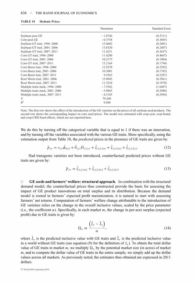
636 / THE RAND JOURNAL OF ECONOMICS
TABLE 10 Hedonic Prices
Parameter Standard Error
Soybean post GE −1.8746 (0.5311)Corn post GE −0.3758 (0.3045)Soybean GT trait, 1996–2000 15.4602 (0.2401)Soybean GT trait, 2001–2006 13.8320 (0.2407)Soybean GT trait, 2007–2011 11.4231 (0.3637)Corn GT trait, 1996–2000 11.4280 (0.4607)Corn GT trait, 2001–2006 10.2175 (0.1904)Corn GT trait, 2007–2011 13.2164 (0.1794)Corn Borer trait, 1996–2000 12.9370 (0.2592)Corn Borer trait, 2001–2006 10.3001 (0.1785)Corn Borer trait, 2007–2011 9.5263 (0.2287)Root Worm trait, 2001–2006 15.0945 (0.2961)Root Worm trait, 2007–2011 11.5234 (0.1978)Multiple traits stack, 1996–2000 −7.5542 (1.6407)Multiple traits stack, 2001–2006 −5.9043 (0.2988)Multiple traits stack, 2007–2011 −4.5185 (0.2994)N 79,260R2 0.686
Note: The first row shows the effect of the introduction of the GE varieties on the prices of all soybean seed products. Thesecond row shows the corresponding impact on corn seed prices. The model was estimated with crop-year, crop-brand,and crop-CRD fixed effects, which are not reported here.
We do this by turning off the categorical variable that is equal to 1 if there was an innovation,and by turning off the variables associated with the various GE traits. More specifically, using theestimation output from Table 10, the predicted prices in the presence of GE traits are given by:
p jm = x jmφt[m] + θc[ j] Dc[ j],m + ζc[ j],t[m] + ζc[ j],l[m] + ζc[ j],b[ j]. (12)
Had transgenic varieties not been introduced, counterfactual predicted prices without GEtraits are given by:
p jm = ζc[ j],t[m] + ζc[ j],l[m] + ζc[ j],b[ j]. (13)
� GE seeds and farmers’ welfare: structural approach. In combination with the structuraldemand model, the counterfactual prices thus constructed provide the basis for assessing theimpact of GE product innovations on total surplus and its distribution. Because the demandmodel is rooted in farmers’ expected profit maximization, it is natural to start with assessingfarmers’ net returns. Computation of farmers’ welfare change attributable to the introduction ofGE varieties relies on the change in the overall inclusive values, scaled by the price parameter(i.e., the coefficient α). Specifically, in each market m, the change in per-acre surplus (expectedprofit) due to GE traits is given by:
�m ≡(
Im − Im
)
α, (14)
where Im is the predicted inclusive value with GE traits and Im is the predicted inclusive valuein a world without GE traits (see equation (9) for the definition of Im). To obtain the total dollarvalue of GE traits in market m, we multiply �m by the potential market size (in acres) of marketm, and to compute the dollar value of GE traits in the entire sample, we simply add up the dollarvalues across all markets. As previously noted, the estimates thus obtained are expressed in 2011dollars.
C© The RAND Corporation 2019.

CILIBERTO, MOSCHINI AND PERRY / 637
The primary inputs for equation (14) are the estimated demand parameters (α,σ1,σ2) andmean farmers’ profits δ jm . Using the predicted hedonic prices with GE traits, and the estimatedterms from the seed demand equations, predicted mean profits with GE traits are given by15:
δ jm = x jm βt[m] − α p jm + ξc[ j],t[m] + ξc[ j],l[m] + ξc[ j],b[ j] + ξ jm, (15)
whereas predicted mean profits without GE traits are given by:
δ jm = −α p jm + ξc[ j],t[m] + ξc[ j],l[m] + ξc[ j],b[ j] + ξ jm . (16)
A feature to note about this procedure is that it involves the modification of characteristicsassociated with GE varieties. As previously noted, by the end of the sample, GE varieties had notonly significantly added to the set of available products, but had also replaced most conventionalofferings.16 In 1996, for example, non-GE varieties comprised 57 out of 66 products; by 2011,they comprised just 38 out of 161 products. If we were to remove GE products entirely fromthe choice set in 2011, that would leave just 38 products available to growers, a number whichlikely underestimates what would have been available in the counterfactual. Maintaining suchan artificial reduction in non-GE products in the relevant counterfactual has the potential tointroduce bias in the estimated welfare gains from GE traits. This is especially problematicin the context of logit models. As noted by Petrin (2002) and Ackerberg and Rysman (2005),among others, the postulated underlying structure implies that an additional option mechanicallyincreases (expected) welfare because it provides another draw from the distribution of randomshocks.17
We address this issue by considering results for four different counterfactual scenarios. Inthe first scenario, we simply remove all the GE products from the choice set of the counterfactualscenario, adjust the prices of the remaining conventional products (as per the hedonic priceregression), and compute the welfare change of seed users accordingly.18 As implied by theforegoing discussion, this approach (labelled the “naive” scenario) is expected to penalize thenon-GE counterfactual and thus inflate the estimated welfare effects.
Alternatively, instead of simply removing GE products from the choice set, we modify thecharacteristics of GE products by removing the GE trait, adjusting the price, and then maintainthis “synthetic” product in the counterfactual choice set if it does not duplicate an equivalentnon-GE product already present. The presumption is that seed manufacturers would have usedthe germplasm currently combined with GE traits to commercialize alternative conventionalseed products instead. For example, suppose that in a given market there are three seed products:Dekalb-GE-corn, Asgrow-conventional-soybeans, and Pioneer-conventional-corn. If we followedthe naive approach, removal of GE traits would drop one product from the choice set (the remain-ing two would be Asgrow-conventional-soybeans and Pioneer-conventional-corn). Instead, withthe proposed alternative counterfactual, we retain three products: the two preexisting conven-tional seed products plus the synthetic Dekalb-non-GE-corn. Implementation of this alternativeprocedure to construct the choice set of the counterfactual requires the resolution of a possibleambiguity. In some markets, after modifying the characteristics of GE products, we can end upwith “duplicates” vis-a-vis the definition of products used in this study, the only difference beingin the unobservable component ξ jm .19 This presents the question of which duplicate product tokeep in the counterfactual choice set. To proceed, we consider two versions of this alternativeapproach. In one case, we keep the duplicate with the largest ξ jm (i.e., the largest mean expected
15 Note that the baseline also uses predicted prices (rather than observed prices), just as the counterfactuals.16 The crowding out of old products due to the introduction of new ones is the main concern of Eizenberg’s (2014)
study of the impact of innovation in central processing units for US personal computers.17 Nevo (2011) provides an extended discussion of this point and notes that the logit model per se is actually not the
source of biased welfare estimates. Rather, the bias may arise from using the logit model to predict counterfactual shares.18 In equation (14), this amounts to an Im , in which the exponential terms for GE products have simply been deleted.19 For example, in a market where we have both conventional Asgrow soybeans and GT Asgrow soybeans, shutting
down the GT traits yields two versions of Asgrow conventional soybean seeds.
C© The RAND Corporation 2019.

638 / THE RAND JOURNAL OF ECONOMICS
TABLE 11 Average Number of Seed Products per CRD, Counterfactual Scenarios
Keep All Keep Best and Keep Conventional Naive
Corn Soybeans Corn Soybeans Corn Soybeans
1996–2000 8.28 6.45 6.42 4.67 6.21 3.722001–2006 14.14 6.76 6.86 5.42 5.59 1.662007–2011 19.95 6.25 7.64 5.65 3.19 0.78
Note: This table reports the average number of products, for both corn and soybeans, under four counterfactual scenarios.See the text for a description of each scenario.
profit for farmers). We call this the “keep best” scenario. In the other case, we keep the duplicatethat was originally a non-GE variety, a situation that we label the “keep conventional” scenario.20
Finally, we also consider the “keep all” scenario, where it is assumed that all synthetic productsobtained from the removal of GE traits in the counterfactual are viable and are therefore kept inthe choice set.
Table 11 reports the average number of products, for both corn and soybeans, that pertainto the foregoing four counterfactual scenarios for each of the three subperiods of the analysis.Comparing the data in Table 11 with the number of products available prior to the advent of GEvarieties, it is clear that the naive and the “keep all” scenarios are not plausible. The naive scenariois associated with a drastic reduction in the number of products, especially for the last subperiod.This is most apparent for soybeans, a reflection of the almost complete adoption of the GT traitin the latter years of the sample. Conversely, the “keep all” scenario displays an artificially largenumber of products, especially for corn.21 Clearly, neither of these two scenarios are likely toproduce credible results. Hence, here we report the counterfactual results only for the other twoscenarios, “keep conventional” and “keep best.”22 We note at this juncture that, by picking theseed product with the largest ξ jm , the “keep best” scenario provides a more conservative estimatedimpact of GE traits on farmers’ expected profit than the “keep conventional” scenario. However,for this very reason, the “keep best” scenario can underpenalize the non-GE counterfactual.Indeed, when the unobserved component for a synthetic non-GE product exceeds that of a(preexisting) conventional non-GE product, then it is possible for the mean expected return ofthis synthetic non-GE product to exceed the expected return of any seed product that existed whenGE products were still available. For this reason, we view the “keep conventional” counterfactualscenario as the most realistic counterfactual.
The first two results columns in Table 12 report the estimated farmers’ welfare gains for thetwo scenarios of interest, and across the three subperiods. For each scenario, we consider threedistinct thought experiments: (i) a market without GE soybean products; (ii) a market withoutGE corn products; and, (iii) a market that excludes GE products in both corn and soybeans. Thethree exercises are helpful in providing insights into whether GE traits affected the two cropsdifferentially.
The first set of results in Table 12 pertains to the entire period 1996–2011. We find that,under the “keep best” scenario, total farmers’ welfare gain from GE innovations is estimated atabout $14.4 billion. It is interesting to note that three quarters of these gains are attributable toone trait: glyphosate tolerance in soybeans. For the “keep conventional” scenario, the estimatedfarmers’ welfare gains are larger, $22.2 billion. The remainder data in the first two results columns
20 In cases where there are duplicate synthetic conventional products, but no preexisting conventional product, wekeep the synthetic conventional product with the highest mean return.
21 From Table 5, in 1996, at the dawn of the GE era, the average number of conventional seed products per market(i.e., CRD) was 3.9 for soybeans and 6.2 for corn. By contrast, for the last subperiod (2007–2011), the naive scenarioentails 0.8 seed products per CRD for soybeans and 3.2 seed products for corn. By contrast, the average number of seedproducts in the “keep all” scenario in the same subperiod was 6.3 for soybeans and 19.9 for corn.
22 We report the full set of results in the Supplementary Information online web Appendix (Appendix D).
C© The RAND Corporation 2019.

CILIBERTO, MOSCHINI AND PERRY / 639
TABLE 12 Farmers’ Welfare Gains and Seed Industry Revenues from GE Traits (2011 $ million)
Farmers’ Welfare Seed Industry Revenues
Period Keep Best Keep Conventional Keep Best Keep Conventional
1996–2011 Soy GE traits 10,019 12,137 7,406 7,211Corn GE traits 3,820 8,704 13,244 15,259All GE traits 14,385 22,199 22,550 25,262
1996–2000 Soy GE traits 1,062 1,796 1,319 1,355Corn GE traits 1 764 668 1,009All GE traits 1,063 2,625 2,019 2,493
2001–2006 Soy GE traits 4,318 5,321 4,043 3,938Corn GE traits 307 2,539 2,581 3,515All GE traits 4,674 8,251 6,940 8,177
2007–2011 Soy GE traits 4,640 5,020 2,044 1,917Corn GE traits 3,512 5,402 9,995 10,734All GE traits 8,648 11,323 13,591 14,592
Note: See the text for a description of “Keep Best” and “Keep Conventional” scenarios. The Supplementary Informationonline web Appendix (Appendix D) reports a fuller set of results, including the two counterfactual choice sets omittedhere (“Naive” and “Keep All”), as well as the estimated counterfactual �m terms ($ per acre of total cropland) used inthe calculations.
of Table 12 investigate how the estimated welfare gains changed over time. Specifically, we alsoreport results for the 1996–2000, 2001–2006, and 2007–2011 subperiods. We see clearly that theestimated welfare gains increased over time, reflecting both increased adoption and rising WTP.
� GE traits and seed industry revenue. Using the estimated counterfactual prices, wecan also infer the additional revenue that accrued to the seed industry due to the ability tocommercialize GE traits. To compute the benchmark seed revenues, we compute the marketshares, and associated value of all seed sold, by using the fitted prices of equation (12) alongwith the estimated seed demand model. For the counterfactual scenario of no GE traits, wecompute predicted market shares by using the counterfactual prices of equation (13), along withthe estimated demand model. We again report results for two scenarios, the “keep best” and “keepconventional.”
The last two columns in Table 12 report the estimated revenues for seed manufacturersattributable to the availability of GE traits. Focusing on the “keep conventional” scenario, wefind that over the entire 1996–2011 period, seed firms’ sales were greater by $25.3 billion, withmore than two thirds of these revenues attributable to the availability of GE corn varieties.Moreover, these revenues from GE traits increased over time, reflecting the increased adoptionof GE seed varieties and, possibly, changing equilibrium pricing conditions (which, again, weare not modelling in a structural way). Over the last five years of our sample (2007–2011), wefind that GE traits boosted seed industry revenue by a total of $14.6 billion, or approximately$2.9 billion per year, with corn contributing significantly more than soybeans to increases in seedindustry revenues. This likely reflects the increase in farmers’ WTP for corn GE traits (possiblyassociated with the commodity price boom noted earlier), as well as the increased diffusion of Bttraits in corn varieties (recall Table 2).
� Discussion. The two approaches we have used to calculate the value of GE traits are basedon different assumptions, as noted earlier. Upon comparing the results in Table 12 with thosein Table 9, however, some common themes are apparent. First, the monetary benefits from GEinnovations are significant. For the last five years of the period analyzed (2007–2011), whenadoption of GE traits was widespread, estimated total surplus was between $3.73 billion per year(Table 9) and $5.18 billion per year for the “keep conventional” scenario (Table 12). We also findthat seed manufacturers have been able to appropriate the larger share of this surplus, although
C© The RAND Corporation 2019.

640 / THE RAND JOURNAL OF ECONOMICS
the structural estimates suggest that it was closer to an even split. Specifically, in the last fiveyears of the sample (2007–2011), the results in Table 9 imply that the seed industry captured75% of the total surplus, whereas the results in Table 12 imply a fraction of 56% (for the “keepconventional” scenario).
It is also of some interest that results differ across soybean and corn seeds. Although farmersreceived the majority of their surplus from soybean GE traits, more total surplus has beengenerated by GE traits in corn, and the seed industry has been able to extract the larger share oftotal surplus in corn. In the final subperiod (2007–2011), Table 9 implies that 100% of the GEtrait surplus created in corn seeds was appropriated by seed manufacturers, whereas in Table 12,this fraction ranges between 74% (“keep best” scenario) and 67% (“keep conventional” scenario).
The estimated seed industry revenue increases due to GE crops, and the estimated increasesin farmers’ expected profits, both measure ex post welfare gains from GE crops. The interpretationis somewhat different, though. For farmers, the figures in Table 12 can be interpreted as net welfaregains: that is, the dollar value of how much better off farmers have been by their ability to purchaseGE varieties—notwithstanding the fact that they had to pay a premium for GE seeds. For theseed industry, on the other hand, increased revenues can be interpreted as ex post returns to pastinvestments in R&D activities.23 Still, comparing the magnitude of gains accruing to farmers andthe seed industry, we see that the latter has been fairly effective at capturing the value createdby GE trait innovations. For example, over the last five years of the sample (2007–2011), forthe “keep conventional” scenarios, farmers’ net welfare increased by $11.3 billion, whereas seedindustry revenue increased by $14.6 billion. Thus, during this period, the seed industry appearsto have been able to capture approximately 56% of the overall monetary value of GE traits.
7. Conclusion
� In this article, we provide an empirical assessment of the value of one of the major innova-tions affecting US agriculture in the last several decades, the introduction of GE traits in US cornand soybeans. Our approach is based on a two-level nested logit model of seed demand, in whichfarmers choose the most profitable option among corn and soybean seed varieties (and an outsideoption). This specification is consistent with the important mechanism of corn-soybean rotationsand it also partially addresses well-known limitations of using the basic logit model to estimatethe welfare impact of new products. The model is estimated using a unique, large data set on UScorn and soybean seed purchases during the 1996–2011 time frame. Using the demand estimates,we find that farmers are willing to pay a significant premium for GE traits, and the extent of thiswillingness has increased significantly over time.
We estimate the total surplus created by the introduction of GE traits, and its distributionbetween farmers and seed manufacturers, with two alternative methods. In the first approach, werecover the total surplus created via the estimated farmers’ WTP for the various GE traits, alongwith observed plantings of GE varieties. With this approach, based on observed price premiabetween GE and conventional varieties, we also compute the additional revenues for the seedindustry due to GE traits embedded into marketed seed varieties (as well as the implied netresidual surplus left for farmers). In the second approach, we use the structure of the estimateddemand model, along with counterfactual prices obtained from a reduced-form hedonic equation,to infer market conditions that would have prevailed had GE traits not been introduced. Ourcounterfactual scenarios are adjusted to account for the fact GE crop varieties gradually crowded
23 The implicit assumption, here, is that the marginal production cost to seed firms for GE and non-GE varieties isthe same. To put our estimates in context, it may be helpful to consider the extent of R&D in this industry. For the five-yearperiod 2007–2011, data reported by Phillips (2014) suggest that the R&D expenditures of the six largest agro-chemicalfirms, for the seed and GE trait segment, amounted to approximately $13 billion. As for individual companies, publiclyavailable data for Monsanto are most informative, because this company’s R&D is almost exclusively devoted to seedsand traits. Monsanto’s annual disclosures to the US Security and Exchange Commission indicate a total of $5.45 billionin R&D expenditures for the 2007–2011 period.
C© The RAND Corporation 2019.

CILIBERTO, MOSCHINI AND PERRY / 641
out conventional varieties. More specifically, rather than simply removing a GE product fromfarmers’ choice sets, we also simulate scenarios in which modified GE products are retainedin farmers’ counterfactual choice sets. In so doing, we avoid the bias that would result fromconflating the removal of the GE technology with an artificial reduction in product diversity.
Our findings suggest that the welfare benefits from GE crops are significant. For the lastfive years of the period analyzed, when adoption of GE traits had reached maturity, estimatedtotal surplus from the two methods discussed ranged from $3.73 billion to $5.18 billion per year.To put matters in context, over this five-year period, total planted acres to corn and soybeansaveraged at 162.7 million per year. Hence, the estimated total surplus due to GE traits reportedearlier ranged from $22.9 to $31.9 per acre of planted crop. We also find that seed manufacturershave been able to appropriate the larger share of this surplus. It is also of some interest that theresults differ across soybean and corn seeds. Although farmers received the majority of theirsurplus from soybean GE traits, more total surplus has been generated by GE traits in corn, andthe seed industry has been able to extract the larger share of total surplus in corn. These results areconsistent with the observation that intellectual property rights have historically played a strongerrole in the corn seed industry. As noted earlier, the commercialization of hybrid varieties, startingin the 1930s, provided the technology to develop improved germplasm as a proprietary asset.Conversely, for soybeans seeds, strong property rights only materialized in the 1990s, with thediffusion of contractual clauses based on newly asserted patent rights (Clancy and Moschini,2017).
Our work has some important implications for the ongoing debate surrounding GE crops.First, our estimates suggest that, at least up to 2011, farmers still obtained significant net benefitsfrom adopting GE crop varieties, notwithstanding the higher seed prices they paid. It is alsonotable that seed firms were able to extract the larger share of the ex post welfare effects ofGE traits. Appropriability of ex post returns from innovation is essential to ensure that firmshave continuing incentives to invest in R&D. This is particularly important in the modern seedindustry, where private R&D funds have vastly exceeded public R&D investments in recent years(Clancy, Fuglie, and Heisey, 2016). Methodologically, our counterfactual approach to estimatingwelfare may be applied to settings in which new products tends to crowd out and replace existingproducts.
Some caveats are also worth noting in closing. Our analysis of the welfare effects of GEcrops pertains to their direct economic consequences for farmers and the seed industry. Welfareimplications arising from possible external effects, such as unintended environmental effects,are obviously not encompassed by our methodology. Also, our framework does not capture thepossible impact of GE trait adoption on crop output prices, which precludes a fuller welfareimpact assessment. Finally, a structural representation of the supply side might be preferableto the reduced-form approach used in this article. This, however, would require a model thataccommodates the complex web of GE trait cross-licensing agreements between seed firms, anundertaking that we leave for future studies.
References
ACKERBERG, D.A. AND RYSMAN, M. “Unobserved Product Differentiation in Discrete-Choice Models: Estimating PriceElasticities and Welfare Effects.” RAND Journal of Economics, Vol. 36 (2005), pp. 771–788.
ALLENBY, G.M., BRAZELL, J.D., HOWELL, J.R., AND ROSSI, P.E. “Economic Valuation of Product Features.” QuantitativeMarketing and Economics, Vol. 12 (2014), pp. 421–456.
ANDERSON, S.P., DE PALMA, A., AND THISSE, J.F. Discrete Choice Theory of Product Differentiation. Cambridge, MA:MIT Press, 1992.
BAFFES, J. AND HANIOTIS, T. “Placing the 2006/08 Commodity Price Boom into Perspective.” World Bank ResearchWorking Paper no. 5371, 2010.
BARROWS, G., SEXTON, S., AND ZILBERMAN, D. “Agricultural Biotechnology: The Promise and Prospects of GeneticallyModified Crops.” Journal of Economic Perspectives, Vol. 28 (2014), pp. 99–119.
C© The RAND Corporation 2019.
642 / THE RAND JOURNAL OF ECONOMICS
BENNETT, A.B., CHI-HAM, C., BARROWS, G., SEXTON, S., AND ZILBERMAN, D. “Agricultural Biotechnology: Eco-nomics, Environment, Ethics, and the Future.” Annual Review of Environment and Resources, Vol. 38 (2013),pp. 249–279.
BERRY, S.T. “Estimating Discrete-Choice Models of Product Differentiation.” RAND Journal of Economics, Vol. 25(1994), pp. 242–262.
BERRY, S., LEVINSOHN, J., AND PAKES, A. “Automobile Prices in Market Equilibrium.” Econometrica, Vol. 63 (1995), pp.841–890.
BIGELOW, D.P. AND BORCHERS, A. “Major Uses of Land in the United States, 2012.” Economic Information Bulletin no.178, US Department of Agriculture, 2017.
BJORNERSTEDT, J. AND VERBOVEN, F. “Does Merger Simulation Work? Evidence from the Swedish Analgesics Market.”American Economic Journal: Applied Economics, Vol. 8 (2016), pp. 125–164.
BULLOCK, D.G. “Crop Rotation.” Critical Reviews in Plant Sciences, Vol. 11 (1992), pp. 309–326.BRADFORD, K.J., VAN DEYNZE, A., GUTTERSON, N., PARROTT, W., AND STRAUSS, S.H. “Regulating Transgenic Crops
Sensibly: Lessons from Plant Breeding, Biotechnology and Genomics.” Nature Biotechnology, Vol. 23 (2005),pp. 439–444.
BRESNAHAN, T.F. “Competition and Collusion in the American Automobile Industry: The 1955 Price War.” Journal ofIndustrial Economics, Vol. 35 (1987), pp. 457–482.
CHARLES, D. Lords of the Harvest: Biotech, Big Money, and the Future of Food. Cambridge, MA: Perseus Publishing,2002.
CLANCY, M., FUGLIE, K., AND HEISEY, P. “U.S. Agricultural R&D in an Era of Falling Public Funding.” Amber Waves, USDepartment of Agriculture, Economic Research Service, 2016.
CLANCY, M.S. AND MOSCHINI, G. “Intellectual Property Rights and the Ascent of Proprietary Innovation in Agriculture.”Annual Review of Resource Economics, Vol. 9 (2017), pp. 53–74.
EIZENBERG, A. “Upstream Innovation and Product Variety in the U.S. Home PC Market.” Review of Economic Studies,Vol. 81 (2014), pp. 1003–1045.
EVENSON, R.E. AND GOLLIN, D. “Assessing the Impact of the Green Revolution, 1960 to 2000.” Science, Vol. 300,no. 5620 (2003), pp. 758–762.
FALCK-ZEPEDA, J.B., TRAXLER, G., AND NELSON, R.G. “Surplus Distribution from the Introduction of a BiotechnologyInnovation.” American Journal of Agricultural Economics, Vol. 82 (2000), pp. 360–69.
FERNANDEZ-CORNEJO, J. “The Seed Industry in U.S. Agriculture: An Exploration of Data and Information on Crop SeedMarkets, Regulation, Industry Structure, and Research and Development.” Agricultural Information Bulletin no.786, US Department of Agriculture, 2004.
FERNANDEZ-CORNEJO, J. AND CASWELL, M. “The First Decade of Genetically Engineered Crops in the United States.”Economic Information Bulletin no. 11, US Department of Agriculture, 2006.
FERNANDEZ-CORNEJO, J., WECHSLER, S.J., LIVINGSTON, M., AND MITCHELL, L. “Genetically Engineered Crops in the UnitedStates.” Economic Research Report no. 162, US Department of Agriculture, 2014.
GELMAN, A. AND HILL, J. Data Analysis Using Regression and Multilevel/Hierarchical Models. Cambridge, UK: Cam-bridge University Press, 2007.
GOEREE, M.S. “Limited Information and Advertising in the US Personal Computer Industry.” Econometrica, Vol. 76(2008), pp. 1017–1074.
GOLDBERG, P.K. “Product Differentiation and Oligopoly in International Markets: The Case of the US AutomobileIndustry.” Econometrica, Vol. 63 (1995), pp. 891–951.
GRAFF, G.D., RAUSSER, G.C., AND SMALL, A.A. “Agricultural Biotechnology’s Complementary Intellectual Assets.”Review of Economics and Statistics, Vol. 85 (2003), pp. 349–363.
GRIGOLON, L. AND VERBOVEN, F. “Nested Logit or Random Coefficients Logit? A Comparison of AlternativeDiscrete Choice Models of Product Differentiation.” Review of Economics and Statistics, Vol. 96 (2014),pp. 916–935.
GRILICHES, Z. “Hybrid Corn: An Exploration in the Economics of Technological Change.” Econometrica, Vol. 25 (1957),pp. 501–522.
HAUSMAN, J.A. “Valuation of New Goods under Perfect and Imperfect Competition.” In T.F. Bresnahan and R.J. Gordon,eds., The Economics of New Goods. Chicago: University of Chicago Press, 1996.
HAUSMAN, J.A. AND LEONARD, G.K. “The Competitive Effects of a New Product Introduction: A Case Study.” The Journalof Industrial Economics, Vol. 50 (2002), pp. 237–263.
HENDRICKS, N.P., SMITH, A., AND SUMNER, D.A. “Crop Supply Dynamics and the Illusion of Partial Adjustment.” AmericanJournal of Agricultural Economics, Vol. 96 (2014), pp. 1469–1491.
HENNESSY, D.A. “On Monoculture and the Structure of Crop Rotations.” American Journal of Agricultural Economics,Vol. 88 (2006), pp. 900–914.
ISAAA. “Global Status of Commercialized Biotech/GM Crops in 2017: Biotech Crop Adoption Surges as Economic Ben-efits Accumulate in 22 Years.” Brief no. 53, International Service for the Acquisition of Agri-biotech Applications,Ithaca, NY, 2017.
LAPAN, H.E. AND MOSCHINI, G. “Innovation and Trade with Endogenous Market Failure: The Case of Genetically ModifiedProducts.” American Journal of Agricultural Economics, Vol. 86 (2004), pp. 634–648.
C© The RAND Corporation 2019.

CILIBERTO, MOSCHINI AND PERRY / 643
MACDONALD, J.M., KORB, P., AND HOPPE, R.A. “Farm Size and the Organization of US Crop Farming.” Economic ResearchReport no. 152, US Department of Agriculture, 2013.
MAGNIER, A., KALAITZANDONAKES, N., AND MILLER, D.J. “Product Life Cycles and Innovation in the US Seed CornIndustry.” International Food and Agribusiness Management Review, Vol. 13 (2010), pp. 17–36.
MCHUGHEN, A. AND SMYTH, S. “US Regulatory System for Genetically Modified [genetically modified organism (GMO),rDNA or transgenic] Crop Cultivars.” Plant Biotechnology Journal, Vol. 6 (2008), pp. 2–12.
Monsanto. “Observations on Competition in the U.S. Seed Industry.” Submitted to the Department of Justice,2009.
MOSCHINI, G. “Biotechnology and the Development of Food Markets: Retrospect and Prospects.” European Review ofAgricultural Economics, Vol. 35 (2008), pp. 331–355.
MOSCHINI, G. “Competition Issues in the Seed Industry and the Role of Intellectual Property.” Choices, Vol. 25 (2010),pp. 1–12.
MOSCHINI, G., LAPAN, H., AND SOBOLEVSKY, A. “Roundup Ready Soybeans and Welfare Effects in the Soybean Complex.”Agribusiness, Vol. 16 (2000), pp. 33–55.
MOSS, D.L. “Transgenic Seed Platforms: Competition between a Rock and a Hard Place? Addendum.” American AntitrustInstitute, 2010.
MUMM, R.H. “A Look at Product Development with Genetically Modified Crops: Examples from Maize.” Journal ofAgricultural and Food Chemistry, Vol. 61 (2013), pp. 8254–8259.
MUMM, R.H. AND WALTERS, D.S. “Quality Control in the Development of Transgenic Crop Seed Products.” Crop Science,Vol. 41 (2001), pp. 1381–1389.
MUSSELLI MORETTI, I. “Tracking the Trend Towards Market Concentration: The Case of the Agricultural Input Industry.”UNCTAD/DITC/COM/2005/16, United Nations Conference on Trade and Development, 2006.
NEVO, A. “Measuring Market Power in the Ready-to-Eat Cereal Industry.”; Econometrica, Vol. 69 (2001),pp. 307–342.
NEVO, A. “New Products, Quality Changes, and Welfare Measures Computed from Estimated Demand Systems.” Reviewof Economics and Statistics, Vol. 85 (2003), pp. 266–275.
NEVO, A. “Empirical Models of Consumer Behavior.” Annual Review of Economics, Vol. 3 (2011), pp. 51–75.NOLAN, E. AND SANTOS, P. “The Contribution of Genetic Modification to Changes in Corn Yield in the United States.”
American Journal of Agricultural Economics, Vol. 94 (2012), pp. 1171–1188.NRC. The Impact of Genetically Engineered Crops on Farm Sustainability in the United States. National Research
Council, Washington DC: National Academies Press, 2010.PERRY, E.D., CILIBERTO, F., HENNESSY, D.A., AND MOSCHINI, G. “Genetically Engineered Crops and Pesticide Use in U.S.
Maize and Soybeans.” Science Advances, Vol. 2 (2016), e1600850.PERRY, E.D., MOSCHINI, G., AND HENNESSY, D.A. “Testing for Complementarity: Glyphosate Tolerant Soybeans and
Conservation Tillage.” American Journal of Agricultural Economics, Vol. 98 (2016), pp. 765–784.PETRIN, A.K. “Quantifying the Benefits of New Products: The Case of the Minivan.” Journal of Political Economy, Vol.
110 (2002), pp. 705–729.PHILLIPS, M. “Directions in Global Research and Development for Crop Protection Products.” Presentation at APVMA
Future Forum, Canberra, Australia, 2014.PRADO, J.R., SEGERS, G., VOELKER, T., CARSON, D., DOBERT, R., PHILLIPS, J., COOK, K., CORNEJO, C., MONKEN, J., GRAPES,
L., AND REYNOLDS, T. “Genetically Engineered Crops: From Idea to Product.” Annual Review of Plant Biology,Vol. 65 (2014), pp. 769–790.
SHI, G., CHAVAS, J.P., AND STIEGERT, K. “An Analysis of the Pricing of Traits in the U.S. Corn Seed Market.” AmericanJournal of Agricultural Economics, Vol. 92 (2010), pp. 1324–1338.
SHI, G., CHAVAS, J.P., AND STIEGERT, K. “An Analysis of Bundle Pricing: The Case of Biotech Seeds.” AgriculturalEconomics, Vol. 43 (2012), supplement, pp. 125–139.
SHI, G., STIEGERT, K., AND CHAVAS, J.P. “An Analysis of Bundle Pricing in Horizontal and Vertical Markets: The Case ofthe U.S. Cottonseed Market.” Agricultural Economics, Vol. 42 (2011), supplement, pp. 77–88.
SOBOLEVSKY, A., MOSCHINI, G., AND LAPAN, H. “Genetically Modified Crops and Product Differentiation: Tradeand Welfare Effects in the Soybean Complex.” American Journal of Agricultural Economics, Vol. 87 (2005),pp. 621–644.
TRAIN, K. Discrete Choice Methods with Simulation. Cambridge, UK: Cambridge University Press, 2009.TRAJTENBERG, M. “The Welfare Analysis of Product Innovations, with an Application to Computed Tomography Scan-
ners.” Journal of Political Economy, Vol. 97 (1989), pp. 444–479.USDA-NASS. 2012 Census of Agriculture: United States, Summary and State Data, Volume 1. Report AC-12-A-51,
United States Department of Agriculture, National Agricultural Statistics Service, 2014.VERBOVEN, F. “International Price Discrimination in the European Car Market.” RAND Journal of Economics, Vol. 27
(1996), pp. 240–268.WRIGHT, B.D. “The Economics of Grain Price Volatility.” Applied Economic Perspectives and Policy, Vol. 33 (2011),
pp. 32–58.WRIGHT, B.D. “Grand Missions of Agricultural Innovation.” Research Policy, Vol. 41 (2012), pp. 1716–1728.
C© The RAND Corporation 2019.

644 / THE RAND JOURNAL OF ECONOMICS
XU, Z., HENNESSY, D.A., SARDANA, K., AND MOSCHINI, G. “The Realized Yield Effect of Genetically Engineered Crops:U.S. Maize and Soybean.” Crop Science, Vol. 53 (2013), pp. 735–745.
Supporting information
Additional supporting information may be found online in the Supporting Information section atthe end of the article.
C© The RAND Corporation 2019.