valuing public goods using happiness data: the case of air quality
TRANSCRIPT

Valuing Public Goods Using Happiness Data: The Case of Air Quality
Arik Levinson
Georgetown University and NBER [email protected]
September 2011
Abstract This paper describes and implements a method for valuing a time-varying local public good: air quality. It matches U.S. survey and air quality data to model respondents’ self-reported happiness as a function of their demographic characteristics, incomes, and the air pollution on the date and in the place they were surveyed. People with higher incomes report higher levels of happiness, and people interviewed on days with worse local air pollution report lower levels of happiness. Combining these two concepts, I derive the average marginal rate of substitution between income and air quality – a compensating differential for air pollution. JEL codes: Q51, Q53, H41 Key words: willingness to pay, stated well-being, pollution, compensating differential Acknowledgments This research is part of a project funded by the National Science Foundation grant #0617839. I am grateful to Resources for the Future for its hospitality during part of the time I worked on the paper, to Emma Nicholson for superb research assistance, to the research staff at the General Social Survey for assisting me with matching confidential aspects of their data to geographic information, to Sarah Aldy for editorial help, and to Chris Barrington-Leigh, Paul Frijters, Carol Graham, John Helliwell, Simon Luechinger, Erzo Luttmer, David Maddison, George MacKerron, Robert Metcalfe, Yew-Kwang Ng, Andrew Oswald, Nick Powdthavee, Karl Scholz, Russell Smyth, Betsey Stevenson, Heinz Welsch and Justin Wolfers for helpful suggestions.

Valuing Public Goods Using Happiness Data: The Case of Air Quality
1. Introduction
Valuing local public amenities and other non-market goods is one of the greatest
challenges facing applied economics. Existing methods, often applied to environmental quality,
include travel-cost models, hedonic regressions of property values, and contingent valuation
surveys in which people are asked directly their willingness to pay for public goods. In this
paper, I describe and test an alternative method for estimating the economic benefit of a local
public good. The fundamental idea is extraordinarily simple. I combine survey, air quality, and
weather data to model individuals' self-reported levels of "happiness," or "subjective well-being,"
as a function of their demographic characteristics, incomes, and the air quality and weather at the
date and place they were surveyed. I then use the estimated function to calculate a compensating
differential for air pollution: the average marginal rate of substitution between annual household
income and air quality that leaves respondents equally happy.
This happiness-based methodology has a number of advantages over existing tools for
valuing environmental quality. The people most averse to air pollution choose to visit and live in
clean locales; as a result, travel-cost and many hedonic models may underestimate the value of
air quality. But because I include county and year fixed effects, coefficients are identified from
daily fluctuations in pollution within a U.S. county and are not subject to these sorting biases.
Because I estimate marginal rates of substitution between income and pollution directly, income
effects do not confound the approach, nor do large gaps between measures of willingness to pay
and willingness to accept. And because I do not rely on asking people directly about
environmental issues, the methodology is not susceptible to the strategic biases and framing
problems of the contingent valuation approach.
Furthermore, although happiness studies have recently been used to estimate tradeoffs
made by public policies, including valuations of public goods and bads, all of the previous work
has relied on annual average values across regions or countries.1 If the public goods are
endogenously determined by regional characteristics also associated with happiness, or if people 1 Public policy issues studies have included price inflation (Di Tella et al. 2001), state cigarette taxes (Gruber and Mullainathan 2005), airport noise (van Praag and Baarsma 2005), inequality (Alesina et al. 2004), urban regeneration (Dolan and Metcalfe 2008), terrorism (Frey et al. 2009), and even air pollution (Welsch 2007; Di Tella and MacCulloch 2008; Ferreira et al. 2006; Luechinger 2009).

2
become habituated to levels of public goods, these studies using annual regional differences in
public goods will yield biased estimates of their value. Air quality, on the other hand, varies
daily within each location, for reasons exogenous to any particular respondent, and presumably
more quickly than people can become habituated.
Naturally, this approach also has disadvantages. It treats responses to questions about
happiness as a proxy for utility and then makes interpersonal comparisons among respondents. It
relies on a vague question about how "things are these days." It identifies the relevant
compensating differential based on trade-offs between fluctuations in daily pollution and
differences among respondents' annual incomes. And it takes household income to be an
exogenous determinant of happiness, rather than potentially determined by happiness. The
reason to pursue this line of research, therefore, is not that it is without shortcomings. Instead, the
attractive feature of this approach is that its shortcomings differ so markedly from those of
standard approaches to valuing public goods, and therefore it serves as a useful point of
comparison.
I present two main results. First, I show that happiness is related in sensible ways to daily
local air pollution. After accounting for respondents' demographics, daily local weather
conditions, as well as local, year, and even month fixed effects, individuals surveyed when the
current local levels of airborne particulates are higher report lower levels of happiness. This first
step is a straightforward empirical exercise. It requires no strong assumptions except the
empirical specification, and I show that the results are robust to a variety of those. I also show
that reported happiness is not sensitive to local levels of undetectable pollutants, such as carbon
monoxide.
The second result uses the estimates from the first part to calculate marginal rates of
substitution between pollution and income, and then computes the respondents' implicit
willingness to pay for improved air quality. This step does involve several strong assumptions,
but I describe those in detail and argue they are no stronger than the assumptions underlying
travel cost, hedonic, or contingent valuation estimates of willingness to pay for air quality.
Moreover, because the assumptions I make differ entirely from the standard set, at a minimum,
the results serve as an alternative to the usual approaches.
Using my preferred specification, I show that people appear willing to sacrifice about $40
for an improvement of one standard deviation in air quality for one day, a figure considerably
3
higher than typical hedonic valuations of air quality and double the value the U.S. Environmental
Protection Agency (EPA) attributes to the economic benefits of the 1970 and 1977 Clean Air
Acts (EPA 1999). One explanation for the large difference is that unlike the EPA approach, the
happiness measure captures aesthetics, lost recreation, and benefits from other pollutants
correlated with particulates.
My analysis yields two important lessons. For environmentalists and environmental
economists, the results provide evidence that air pollution, in addition to detrimentally affecting
health and property, has a direct negative effect on people's stated well-being, as well as
evidence that the monetary value of that effect may be quite large. For the growing literature on
happiness and economics, the results provide yet another piece of evidence that subjective well-
being varies in sensible ways with respondents' observable characteristics and circumstances.
2. Happiness in economics
Happiness has enjoyed a recent surge of serious attention from economists. Much of the
academic and popular happiness literature addresses the decades-old findings of Easterlin
(1974): stated happiness does not increase with income across countries, or within a country over
time, but it does increase with income across individuals within a country at any given point in
time. Some recent work challenges the first part of this Easterlin Paradox, showing that
happiness increases with GDP per capita across countries in expected ways (Stevenson and
Wolfers 2008; Deaton 2008; Helliwell et al. 2009). But the second part remains unchallenged:
stated happiness has not increased over time as per capita incomes have increased (Oswald 1997;
Layard 2006). This paradox has two obvious interpretations. One is that people become
habituated to their situations and change their reference level of well-being.2 Another is that
happiness depends on relative income—the richest man in a poor town may be happier than the
poorest man in a rich town, even if the rich man is poorer in absolute terms.3
2 Kahneman (2000) writes about individuals having a base level of stated well-being, which major life events (divorce, injury) perturb at most for a few years. Others, such as Oswald and Powdthavee (2008), show incomplete recovery of happiness after such events. Graham (2009) provides evidence that people become habituated to crime, corruption, democracy, and health. 3 See Luttmer (2005). Also, recent work suggests this relative interpretation may be optimal from an evolutionary standpoint (Rayo and Becker 2007).

4
Under either interpretation, the Easterlin Paradox has implications for using happiness to
measure willingness to pay for public goods. If happiness does not increase with income across
regions or over time, it would seem unlikely to vary with the level of any particular public good.
For income, happiness increases relative to other people in the same locale at the same time. The
analog for pollution is that happiness will increase with air quality relative to the current regional
norm, but not relative to other regions or within regions over long periods of time.4 That is why a
key feature of this analysis identifies happiness as a function of the place-specific, date-specific
air quality, at the place and date where the happiness question was asked. In other words, I
compare stated happiness by statistically similar respondents, at the same locale, during the same
season of the same year, who just happen to have been surveyed on days when the air quality
differed.
While much of the economics literature on happiness focuses on deep questions about the
rationality of economic actors, interpersonal comparisons of ordinal utility functions, and links
between economics and psychology, economists are also attempting practical, policy-relevant
applications.5 Recent work uses happiness surveys to evaluate people's willingness to trade
unemployment for inflation and argue that central bankers place too much emphasis on
combating inflation (Di Tella et al. 2001), examine the welfare consequences of German
reunification on different groups (Frijters et al. 2004), assess the degree to which state cigarette
taxes make smokers better off by helping them quit (Gruber and Mullainathan 2005), and
estimate the degree to which the marginal utility of consumption increases or decreases when
people become ill (Finkelstein et al. 2008). Happiness measures have also been used to try to
place a monetary value on airport noise (van Praag and Baarsma 2005), flood disasters
(Luechinger and Raschky 2009), terrorism (Frey et al. 2009), and weather and climate (Rehdanz
and Maddison 2005; Becchetti et al. 2007; Barrington-Leigh 2008). All use annual average
measures of the public good (or bad), raising the possibility that endogeneity or habituation
biases their answers.
Several papers close in spirit to this one use happiness measures to value air quality.
Welsch (2002, 2006, 2007) estimates values of willingness to pay for air quality using various
4 As one reviewer has noted, this issue should also be a concern for hedonic estimates of compensating differentials. If owners of homes in polluted regions become habituated to their circumstances, those houses may have smaller measured compensating differentials. 5 These practical applications raise concerns among critics. Smith (2008) writes, "[T]he [happiness economics] train is precipitously close to leaving the station and heading for use in full-scale policy evaluation."

5
cross-sections and panels of country-level data. The 2006 paper, for example, estimates that the
reductions in nitrogen dioxide and lead pollution in Europe from 1990 to 1997 were worth
$1,200 per capita and $2,200 per capita, respectively, in 2008 dollars. Di Tella and MacCulloch
(2008) regress happiness on income and the national, annual, per capita emissions of sulfur
dioxide (SO2), and show that an increase of one standard deviation in SO2 correlates with a
decline in happiness equivalent to a 17 percent reduction in income. As first uses of happiness
data to estimate willingness to pay for air quality, these works break new ground. However, they
also share a drawback common to this literature—they use average annual national measures of
air quality. Aggregating environmental quality across entire countries masks much of its
heterogeneity. The standard deviation of particulate air pollution in the U.S. is twice as large if
we look at daily observations within states instead of averages across states or years.
Two recent papers avoid the problems associated with inter-country comparisons of
happiness by looking across regions within Ireland (Ferreira et al. 2006) and Germany
(Luechinger 2009). Luechinger uses annual mean concentrations of SO2 at 533 monitoring
stations in Germany over a 19-year period. To control for sorting by individuals into different
locales, he cleverly instruments for air quality using respondents' locations upwind and
downwind of large power plants that installed SO2 emissions control equipment. Luechinger
finds a marginal willingness to pay of $232 for a one microgram per cubic meter (μg/m3)
reduction in SO2, while average SO2 concentrations fell by 38 μg/m3 over the time period.6
In theory, all the prior work using happiness to value public goods, air quality included,
could suffer from a version of the Easterlin Paradox. If happiness does not increase
systematically with income across countries or over time, we should be surprised if it increases
with public good levels across countries or over time, perhaps because people become
habituated. In that case, it seems unlikely that happiness questions can be used to value public
goods using data on aggregate yearly or national public good levels.
Two final issues contrast most prior attempts to value air quality using happiness data.
First, work based on cross-country pollution differences faces the problem that it compares
survey questions asked in various languages and cultures, where notions of happiness may differ.
Second, air pollution and weather are highly correlated. Studies of happiness and weather omit
pollution (Rehdanz and Maddison 2005; Barrington-Leigh 2008), while studies of happiness and
6 €183 in 2002, converted to 2008 dollars using the average 2002 exchange rate and the CPI-U-RS.

6
pollution omit weather (Welsch 2007; Luechinger 2007; Di Tella and MacCulloch 2008). To
date, none have included both, a potentially important source of omitted variable bias.
This paper solves these problems. It focuses entirely on the United States, so fewer
language and cultural differences complicate the responses to questions about happiness. It
controls for the current local temperature and precipitation, both of which are likely to be
correlated with happiness and pollution. Instead of aggregate national or yearly measures of
pollution, it uses the environmental quality at the time and in the location where the happiness
survey question was asked. Time and place fixed effects can account for relative differences in
happiness, and the measured effect of pollution on happiness will be relative to similar
respondents who were interviewed in the same place during the same month, but happen to have
been interviewed on a day when the air quality differed.
3. Data and methodology
For happiness measures, I rely on the General Social Survey (GSS), which the National
Opinion Research Center conducts annually.7 Several thousand U.S. respondents are interviewed
in person each year, usually in March. The key GSS question asks, "Taken all together, how
would you say things are these days? Would you say that you are very happy, pretty happy, or
not too happy?" This question forms the basis for the dependent variable. In addition to asking
about happiness, the GSS contains the usual demographic information, including age, household
income, race, education, sex, marital status.8
Importantly for this purpose, the GSS contains the date each respondent was questioned. I
have obtained from the GSS staff the confidential codes identifying the county or city in which
each respondent was surveyed. Knowing the date and place allows me to match the GSS to the
particular air quality on the day and in the place where the survey was administered.
For air quality information, I turn to the EPA's Air Quality System (AQS). The AQS
contains the raw, hourly, and daily data from thousands of ambient air quality monitors
7 More information about the GSS can be found at http://www.norc.org/GSS+Website/ (accessed July 26, 2010). 8 The GSS income variable is categorical, and the categories change periodically. But the GSS includes numerous categories each year (21 in 1993) and converts these into real values by taking the midpoints of the ranges and adjusting for inflation and top coding. I use the GSS reported real income (Ligon 1989). I also test an instrument for income using the reported incomes of randomly selected Current Population Survey participants with similar characteristics.

7
throughout the United States. The data include the geographic location of each monitor, the types
of pollutants monitored, and the hourly observations.9 For current local weather conditions, I use
data from the National Climate Data Center, which reports daily temperature and rainfall at each
of the thousands of weather monitoring stations throughout the United States.
To merge the survey data with the weather and air quality data, I take the population-
weighted centroid of the GSS respondent's county and draw an imaginary 25-mile circle around
it. I then take a weighted average of all the air quality and weather monitors within the circle,
where the weights are equal to the inverse of the square root of their distance to the population-
weighted centroids.10
The air quality monitors contain data on ambient concentrations of criteria air pollutants,
but not all data are available in all places or during all time periods. Carbon monoxide (CO), for
example, does have consistently measured data in many locations going back to the early 1970s.
However, CO is odorless and invisible, and I would not expect it to affect happiness responses in
survey data. Airborne particulates, on the other hand, cause physical discomfort, especially
particles smaller than 10 micrometers (PM10). In addition, small particles form visible haze that
reduces visibility and may affect people aesthetically. The AQS contains PM10 readings
beginning in the mid-1980s, so I begin this analysis in 1984.
For particulates, monitoring stations only record ambient concentrations every six days.
As a result, many of the happiness survey questions were asked on days when no nearby air
quality monitors recorded data. Moreover, in any given location, different days may be recorded
by different sets of nearby monitoring stations. To smooth out this variation and use as many of
the happiness survey responses as possible, I interpolate between six-day observations for each
monitoring station. In the robustness checks below, I also report results for the subset of
monitoring stations with actual, uninterpolated values.
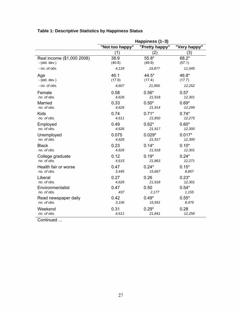
Table 1 presents some descriptive statistics for the GSS, broken out by happiness
response. People with larger annual incomes are more likely to have higher levels of happiness.
9 Recent years are available on the AQS Web site, earlier years by special request to the EPA. More information about the AQS can be found at http://www.epa.gov/ttn/airs/airsaqs (accessed July 26, 2010). 10 Other weights, such as a simple average of all the monitors in a county, yield similar results. The GSS has surveyed about 275 areas, and the names given to these areas do not typically correspond to U.S. Census or U.S. Postal Service names. The GSS geographic codes sometimes correspond to individual cities, sometimes to counties, and occasionally to multi-county areas. (This last group is dropped). I first translated the GSS place names to Census county codes by hand, then assigned each county its population centroid, and merged those with the data from the weather and pollution stations within 25 miles.

8
(Asterisks indicate statistically significant differences from the column to the left.) Note that this
does not contradict the Easterlin Paradox, as most of the income variation is across individuals
within years. Other demographic variables correlated with happiness include marital status, age,
employment and unemployment, race, education, and health.
Methodology
I estimate versions of the following function:
, (1)
where Hijt is the stated happiness of respondent i in location j at date t. The variable Pjt is the air
pollution at location j at date t. The log of income (lnYi) conveniently captures the declining
marginal effect of income on happiness, consistent with typical papers estimating happiness
functions, and it translates directly into an increasing marginal willingness to pay for air quality
(which I test explicitly later).11 Below I show that the estimated trade-offs between pollution and
income are unchanged if I substitute the log of pollution, the level of income, or ordered probit
versions of those; include multiple interactions; or estimate a binomial probability that Hijt > H*
for an arbitrary H*. This robustness to empirical specification is especially important given the
limited reporting categories for the happiness variable in the GSS. The vector Xi contains a set
of other socioeconomic characteristics of respondent i, δj is a location-specific fixed effect, and
ηm is a month fixed effect.
Once estimated, I can totally differentiate the function, set dH=0, and solve for the
average marginal rate of substitution between pollution and income, ∂Y/∂P:
0
ˆ
ˆ|dH
YY
P
, (2)
the amount of annual income necessary to compensate for a one-unit increase in air pollution.12
To avoid the cumbersome phrase "average marginal rate of substitution," henceforth I will use
11 If happiness successfully proxies for utility, we would expect diminishing marginal happiness/utility. Happiness as reported to the GSS, in three discrete categories, may not follow the same distribution. In what follows I show that the estimates are robust to a variety of functional form assumptions for equation (1). Using the log of income also avoids the unattractive feature of exponential functional forms in that the marginal rate of substitution does not become undefined in the middle of the relevant range. See Layard et al. (2008) for alternatives. 12 Naturally, alternative formulations of (1) lead to different expressions for willingness to pay in (2). For example, using the level of income instead of its log means that, conveniently, ∂Y/∂P is simply the ratio of the coefficients on
pollution and income, ˆ ˆ .
ln 'ijt jt i i j m ijtH P Y X

9
the term "willingness to pay" (WTP), fully recognizing that equation (2) represents no one
person's stated willingness. Rather, it represents an estimate of the trade-offs between income
and air quality that will leave people, on average, equally happy.
Some theoretical and practical concerns
Using equation (2) to measure marginal rates of substitution involves placing some strong
assumptions on the underlying utility functions. We typically assume individuals make choices
as though they are maximizing some unobserved utility function, observe market prices and the
choices people make, and infer from those prices and choices properties of their underlying
utility functions, such as risk aversion, impatience, and altruism. The fundamental challenge
facing economists valuing public goods is that we do not observe market prices or choices.
Public goods such as air quality have no markets, and individuals cannot "choose" their own
level of public goods directly, except by voting or relocating. So instead, this analysis proposes
turning the typical economics around. We will observe utility, or a proxy for utility, and infer
what choices people would be willing to make and what prices would therefore be optimal.
The first problem with this approach is that "happiness" as recorded by questions on
surveys is not utility. Kahneman (2000) addresses this, distinguishing between "decision utility,"
which is economists' notion of the underlying individual welfare function that drives economic
choices, and "experience utility," something closer to stated happiness, experienced moment to
moment. We do not observe either type of utility directly; in fact, the survey questions are not
clear about which they seek, asking only how happy people are "these days." Perhaps the easiest
way to think about this methodology is that it uses respondents' stated happiness as a proxy for
their utility, or as an observable manifestation of latent utility. As long as respondents with
higher latent utility are more likely to say they are happier, this approach is consistent with a
wide variety of discrete choice models in economics.
Another potential concern about the proposed approach is that the question the GSS asks
is unclear about what length of time "these days" refers to. If the question is about general well-
being spanning several months or years, it should not be influenced by temporary changes, such
as the current daily level of air pollution relative to a regional seasonal norm. Psychologists and
economists have found, however, that people tend to respond based on contemporaneous
circumstances. Schwarz and Strack (1991) describe how people interviewed after making a

10
photocopy were significantly more satisfied with their lives if they found a dime on top of the
copy machine. Clark and Georgellis (2004) test whether reported "job satisfaction" proxies for
"experience utility." They find that current and lagged values of reported job satisfaction predict
the likelihood British laborers will quit, suggesting that reported satisfaction has a current
component.
In other words, people who are asked about their overall satisfaction with life in general
respond in a way that is sensitive to current conditions. I wish, in retrospect, that the GSS had
asked people two happiness questions: one about their overall life satisfaction, and one about
their happiness at the moment the question is asked. The second question would identify the
effect of contemporaneous local pollution. Given that the survey only asks how things are "these
days," it is fortunate that people seem to respond as if they had been asked the momentary
happiness question, in a way that is useful for valuing current levels of air quality.
A third likely objection to this approach is that economists normally assume utility is
ordinal, rather than cardinal, and that interpersonal comparisons based on stated happiness are
impossible. If an unpolluted day moves person #1 from "not happy" to "very happy," and person
#2 from "not happy" to "pretty happy," that does not mean that person #1 gets more utility from
clean air than person #2, or that person #1 would be willing to pay more for clean air. Put
differently, we could alter some people's happiness functions by a positive monotonic
transformation, while leaving others' unchanged, and it would yield the same rank ordering of
outcomes for each individual. It would not, however, yield the same estimates of equation (1).
Economists studying happiness have responded to this concern in several ways. Some,
like Ng (1997), have argued that ordinal utility is an overly restrictive assumption, and that
ample evidence shows people's utilities are interpersonally comparable and cardinal. Others have
implicitly assumed that happiness is ordinal but interpersonally comparable. In other words, if
the latent utility of person #1 is higher than that of person #2, then the stated happiness of person
#1 will be higher than that of person #2. This allows researchers to estimate an ordered discrete
choice model, such as an ordered logit or probit. Alesina et al. (2004), Blanchflower and Oswald
(2000), and Finkelstein et al. (2008) follow this empirical approach. Most researchers who have
applied both approaches have found little difference between the results of a linear regression

11
and an ordered logit or probit (Ferrer-i-Carbonell and Frijters 2004).13 Since I am not interested
in the marginal utility of income or air quality separately, but only the ratio of the two as in
equation (2), my analysis is less sensitive to these issues. I show below that the estimate of
equation (2) is robust to a wide variety of empirical specifications.
Finally, economists should be concerned that income is endogenous with respect to
happiness. While more income may make people happier, inherently happier people may earn
higher incomes. Very few papers address this. Luttmer (2005) instruments for household income
using interactions between the respondents' and spouses' industry, occupation, and location.
Powdthavee (2009) uses time series data on the number of household members working.14 Both
find that the income coefficient in IV specifications is much larger than in OLS specifications—
three times larger in Luttmer's case. This suggests that equation (2) will overstate the marginal
WTP for air quality. Unfortunately, the GSS is not a panel, so I cannot employ either author's IV
strategy. Instead, I try one specification where I instrument for income using randomly-selected
Current Population Survey incomes for respondents from the same year and state and of the
same age, sex, education, and marital status, yielding slightly smaller estimates of WTP.
In the end, my focus is on obtaining convincing evidence for the effect of pollution on
happiness, based on exogenous daily variation, and then using that cautiously to infer a marginal
WTP. All I can do is remain cognizant of these strong assumptions, remind readers that standard
approaches to valuing environmental quality—travel costs, hedonics, contingent valuation—have
their own sets of strong assumptions, and demonstrate that the robust results obtained from this
approach yield plausible valuations and sensible differences for various subsets of the sample
population.
4. Results
Table 2 begins by estimating versions of equation (1). The first column excludes every
right-hand side variable except income and daily local pollution, measured using particulates
(PM10). Happiness increases with annual income and decreases with pollution on the day of the
interview. The coefficients suggest that a 10 μg/m3 increase in local daily particulates is
13 One key advantage of the regression approach over the ordered probit is that the former can include fixed effects, so any individual or region-specific norms for happiness can be differenced out. 14 Gardner and Oswald cleverly circumvent the endogeneity by examining the mental wellbeing of lottery winners.

12
associated with a decrease in happiness of 0.014, on a three-point scale. The log income
coefficient suggests that a 10 percent increase in annual income is associated with an increase of
happiness of 0.013, on a three-point scale. However, since happiness may be regarded as only
ordinal (or a proxy for utility which is ordinal), I do not want to overemphasize the absolute
magnitudes. More important is the ratio of the two coefficients, or the trade-off between
pollution and income that leaves people at the same level of happiness.
To place a dollar value on air pollution, we need to calculate equation (2). Plugging in
−0.0014 for ̂ , 0.132 for ̂ , and 42.3 for the mean income (in $1,000s), the WTP is ∂Y/
∂P=$459, as reported at the bottom of Table 2.15 In other words, a one μg/m3 increase in PM10,
on the day of the interview, reduces an average person's stated happiness by an amount equal to a
$459 decline in annual income. What does this mean? This is where some ambiguity arises.
The $459 figure represents an estimate of the amount of annual income that increases
happiness (at the mean log income in the sample) by the same amount as a one μg/m3 reduction
in PM10 pollution, but the PM10 coefficient is identified from daily fluctuations in air quality. If
we divide the $459 by 365 days, we get an estimate of $1.26 per day. To put this into context,
note that the standard deviation of PM10 is 14.4 μg/m3. Our estimate, then, corresponds to a
WTP of $18 (14.4×$1.26) for a one-standard-deviation improvement in air quality, for one day.
Column (2) of Table 2 adds the average particulate count for each respondent's location,
for the month in which the survey was taken. Now the daily PM10 measure is identified from the
difference between air quality on the day of the survey and the prevailing conditions that month.
The monthly coefficient is statistically insignificant. One interpretation is that the monthly values
are merely imprecise measures of the daily values, which is what people really care about.
Another is that people become habituated to their environmental circumstances and respond only
to daily departures from the local norm.16 The daily coefficient increases, suggesting a WTP of
$21 rather than $18. Column (3) adds year, month, and county fixed effects.17 These do not
15 The mean real (2008) household income for the 6,035 observations in Table 2 is $62,000. But the mean log income, where income is in thousands, is 3.75, which corresponds to $42,000. 16 The standard errors on the monthly values are large, meaning we cannot differentiate between these interpretations. Monthly fixed effects, added next, also account for seasonal effects. If people are happier in spring, say, and particulates are lower in the spring, that would bias the results absent monthly fixed effects. 17 Note that this standard deviation of 14.4 μg/m3 represents variation both across and within year-month-county "cells." The average standard deviation within cells is 5.7 μg/m3. The sample includes an average of 774 observations per year, 2,298 per month, and 142 per county. The average year-month-county cell has 10 observations, ranging from 1 to 59.
13
change the basic findings, and the year and location fixed effects (unreported) are statistically
insignificant, an unsurprising result given the Easterlin Paradox.
Finally, column (4) adds a battery of demographic and local covariates. Happiness
decreases and then increases with age, falling to a minimum at about age 40. Women and people
who are married, not unemployed, and healthy are happier. Happiness rises with temperature at
low temperatures, falls with temperature at high temperatures, and rises in the difference
between the daily maximum and minimum, which proxies for cloud cover or humidity. All these
results conform with standard findings in this literature. More importantly, none change the basic
result that happiness increases with income and decreases with local daily pollution. If anything,
the demographic variables halve the coefficient on income, thereby doubling the estimate of
WTP to $38 for a change of one standard deviation in PM10.
Table 3 presents a sample of some alternative specifications. Column (1) uses the level of
income rather than its log. Nothing changes except the formula for calculating WTP (See
footnote 12). Column (2) uses both the log of income and the log of PM10, again with no
meaningful change in the calculated WTP. Column (3) estimates equation (1) as an ordered
probit. Column (4) estimates a probit where the dependent variable is an indicator for the highest
happiness response, with little change to the measured trade-off between pollution and income,
though the estimated WTP is somewhat higher at $65.18 Table 3 thus demonstrates that
respondents' stated happiness varies systematically with their incomes and the local daily air
quality in ways that are robust to a variety of empirical specifications.
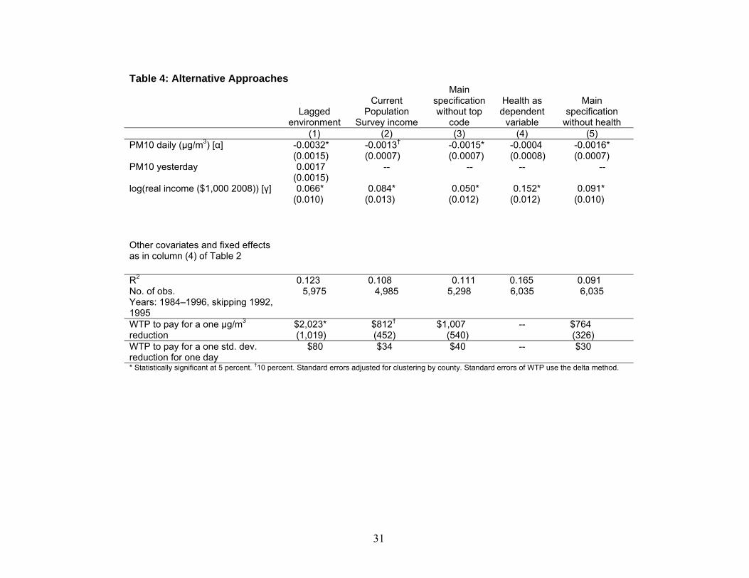
Table 4 addresses some deeper issues with the approach. Column (1) includes a control
variable for the PM10 count the previous day, to account for the possibility that the effects of
pollution on happiness may be cumulative. The coefficient on yesterday's pollution is positive
and insignificant, but its inclusion increases the negative effect of the current day's air pollution
on happiness, resulting in a larger measured WTP. However, given the high degree of correlation
between the two air quality measures, the point estimate of WTP over the two-day period is
about the same as for the basic specification in Table 2.
Column (2) of Table 4 addresses two concerns about the measure of respondents'
incomes. First, the GSS asks respondents to place their household incomes into categories
18 I also estimated versions of equation (1) as both linear probabilities and probits that H>1 and H>2, respectively, again with the same results.
14
representing income ranges, rather than asking them to report their actual incomes, and the
income ranges change periodically. The categorical responses were converted by the GSS into
intertemporally consistent values by taking the midpoint of each range and adjusting for
inflation. However, because there are more than 20 categories, this first concern is not
particularly worrisome. A second, deeper issue involves the endogeneity of income. Happiness
and household incomes are correlated, but we do not know if that is because income causes
happiness, or because happy people earn higher incomes. To address both issues, I match each
GSS respondent to a randomly selected Current Population Survey respondent from the same
state and year and with the same age, sex, education, and marital status as the GSS respondent.
The coefficient on this instrumented income variable (0.084), reported in column (2) of Table 4,
is larger than in the basic specification in column (4) of table 2 (0.066), consistent with Luttmer
(2005) and Powdthavee (2009), resulting in a somewhat smaller WTP for air quality.
Column (3) of Table 4 addresses the concern that 12 percent of the observations are top
coded. Dropping those observations with incomes in the top brackets yields estimates nearly
identical to the baseline specification in table 2 that includes those observations.
Columns (4) and (5) deal with concerns about the health status variable (four categories
ranging from "excellent" to "poor"). If people's self-reported health status varies daily, as a
consequence of changes in pollution, then the health and pollution variables in part measure the
same thing, and the WTP calculation in equation (2) that omits health will be biased. To check
this, in column (4), I estimate a version of equation (1) with health status as the dependent
variable, rather than happiness. Here, the coefficient on daily PM10 is small and insignificant,
suggesting that people respond to the GSS health question based on their long-term health
characteristics, not daily variations. To be certain, in column (5), I estimate a version of equation
(1) without the health variables. The pollution coefficient is unaffected, but omitting the health
variables, which are negatively correlated with both income and happiness, leads to a higher
income coefficient and a correspondingly somewhat smaller estimated WTP.
Table 5 estimates the basic specification from column (4) of Table 2 for alternative
measures of air quality. First, the results so far use air quality measures that interpolate between
readings that occur every six days. As an alternative, I tried using only those observations where
a true uninterpolated reading was available for a nearby station. Those results are summarized in
column (1) of Table 5. The effects of pollution and income on happiness are both slightly larger

15
than in the basic specification, leading on balance to a nearly identical estimate of WTP for a one
μg/m3 reduction in PM10 ($969). Because the variance across the uninterpolated values is higher
than for the interpolated values (18.2 μg/m3 rather than 14.4 μg/m3), the WTP for a change of
one standard deviation is slightly higher at $48.
Column (2) of Table 5 estimates equation (1) for ozone. Here, the coefficient on pollution
is negative but statistically insignificant. The point estimate of WTP for a change of one standard
deviation is $11. My initial expectation was that the ozone coefficient would be significant, since
ozone is associated with aesthetically unpleasant brown skies. However, because the GSS is
collected mostly in March, when ozone is not typically a problem, I may be unable to identify an
ozone effect with these data.
Column (3) reports results for SO2. This is the pollutant Luechinger (2009) studied, using
annual averages for SO2 upwind and downwind from power plants. In my case, the SO2
coefficient is statistically insignificant, and the point estimate leads to a WTP of $9, much less
than the WTP for reductions in PM10. The different result may stem from the fact that SO2 is
less ubiquitous than PM10. SO2 poses a particular problem downwind of coal-fired electric
power plants. By focusing on respondents in the neighborhood of such plants, Luechinger was
able to identify an SO2 effect. My study covers many areas without significant SO2 problems.
Column (4) of Table 5 reports results for carbon monoxide. Again the coefficient on CO
is statistically insignificant, and the point estimate, for a change of one standard deviation, is
$13. Because CO is both odorless and colorless, any effect of CO on reported well-being would
necessarily be the result of its correlation with omitted covariates.
Finally, columns (5) through (7) of Table 5 run the basic specification for PM10, but also
include daily measures of Ozone, SO2, and CO, respectively. In each case, the PM10 coefficient
is essentially unaffected, the additional variable is statistically insignificant, and the WTP for a
one-standard-deviation change in PM10 stays within the same range—between $34 and $49.
Magnitudes
So far, I have been discussing WTP for a one-standard-deviation change in pollution,
which amounts to 14.4 μg/m3 for the interpolated PM10 measurements. How large is this
change? The average PM10 reading in the sample is 30.4 μg/m3, so one standard deviation
constitutes a 50 percent change in pollution.
16
Perhaps a more relevant benchmark compares the value of air quality from this new
estimate to those of the traditional approaches. The EPA (1999) publication Benefits and Costs of
the Clean Air Act estimates that the 1970 and 1977 Clean Air Act Amendments reduced ambient
particulate matter by an average of 45 percent nationally. This improvement in air quality is
predicted to have reduced premature mortality, chronic bronchitis, days with respiratory
symptoms, and lost work days, each of which is assigned a monetary value based on the existing
economics literature valuing health costs and statistical lives. The total benefit of just those
improvements due solely to the reduction in particulate matter is slightly more than 1.6 trillion
2008 dollars, or $6,880 per capita, or $19 per day per person.19 By comparison, the value of $38
per day in Table 2 does not seem out of the question because the happiness approach
incorporates all the effects in the EPA study, as well as aesthetic values, ecological effects, non-
monetized health effects, altruism, and any immediately observable consequences of multiple
pollutants correlated with PM10.
An alternative to using health and mortality would be the hedonic method. Smith and
Huang (1995) conduct a meta-analysis of this literature and find an average marginal WTP for a
one μg/m3 reduction in total suspended particulates of $226 (in 2008 dollars). A 14.4 μg/m3
increase would be worth $3,254, which amortized at 5 percent comes out to $163 per year, or
considerably less than $1 per day. More recent work by Chay and Greenstone (2005) uses an
instrumental variables approach to compare housing values in U.S. counties according to
whether they are in compliance with National Ambient Air Quality Standards and finds that
housing values in non-compliance counties grew by an average of $2,774 between 1970 and
1980 (in 2008 dollars) due to the Clean Air Act.20 Amortized at 5 percent, this amounts to $137
per year, comparable to the Smith and Huang numbers, but considerably smaller than those in
the EPA analysis of the Clean Air Act or these results using happiness data.
Probably the most controversial methodology for valuing environmental quality is
contingent valuation, which asks respondents directly to place monetary values on environmental
changes. The EPA uses a version of this approach in calculating the benefits of the Clean Air
Act, in that the monetary benefits of reduced mortality and morbidity come from contingent
19 Calculations based on Tables ES-1 and ES-3 in EPA (1999), adjusted for inflation using the CPI-U-RS, and a 1990 48-state U.S. population of 247 million. 20 Kim et al. (2003) find a nearly identical value ($2,333) for a 4 percent decline in mean ambient SO2 concentrations.

17
valuation studies. One could imagine, however, asking directly about air quality. A seminal
example of this approach is an EPA-sponsored evaluation of air quality in California (Loehman
et al. 1985). They asked respondents whether they would vote to improve air quality by 30
percent, along with associated health and visibility, at various costs, and showed them
photographs of the sky with clean and dirty air. While not directly comparable to the 14.4 μg/m3
improvements discussed above, the average annual WTP was $980 in Los Angeles and $251 in
San Francisco (in 2008 dollars), again considerably less than the EPA's values or those in Table
2.
One possible explanation for why the estimates in this analysis are so much larger than
typical damage estimates for air pollution is that I treat household income as exogenous. The
solution, instrumenting for household income, is conceptually difficult, especially because I have
no time-series variation in respondents' incomes. For instruments, we need exogenous changes in
income that have no independent effect on happiness. Powdthavee (2009) does have panel data,
and he instruments for respondents' household incomes using changes over time in the number of
household members working. He finds that the coefficient on household income doubles.
Luttmer (2005) instruments for household incomes using the respondents' and spouses' industry,
occupation, and location, taking advantage of the fact that he has a panel of respondents over
time. Respondents who work in occupations and industries where the average wage grows, or
whose spouses work in such occupations and industries, are likely to experience higher
household incomes themselves and are therefore more likely to report higher levels of happiness.
Using this instrument, Luttmer finds the coefficient on happiness is three times as large as when
he uses household income directly. This suggests I should divide the estimated WTP of $38 per
day by three. The result, $13 per day, or $4,750 per year, is lower than the EPA (1999) estimate,
but still considerably higher than the hedonic or contingent valuation estimates.
Robustness and interactions with other demographics
One natural test of whether these results truly measure reactions to air pollution, and not
some spurious covariate, is to check whether they vary sensibly with respondents' characteristics.
A natural candidate is income. If environmental quality is a normal good, we would expect WTP
to increase with income. To test this directly, I include an interaction between the income
variable and the daily PM10 count. To ensure that the coefficient α1 can be interpreted in the
18
same way as previously, at the average income, I interact pollution with the difference between
the respondent's log income and the mean log income in the sample. Bars above variables denote
means.
1 2 ln ln ln 'ijt jt jt i i i j m ijtH P P Y Y Y X . (3)
Results are reported in the first column of Table 6. The pollution coefficient is unchanged by the
inclusion of the interaction, and although the interaction term's coefficient ( 2̂ ) is not
statistically significant, the two terms together ( 1̂ and 2̂ ) are jointly significant, and the
interaction coefficient is negative, suggesting that higher-income individuals are willing to pay
more for clean air.
The marginal rate of substitution between income and air quality in this case, for the
average level of pollution and log income, is
1 2
0 2
ˆ ˆ (ln ln )
ˆ ˆ|dH
Y YYY
P P
. (4)
As shown at the bottom of Table 6, the point estimates in column (1) are such that people in the
25th percentile of the GSS income distribution appear willing to pay $32 for a change of one
standard deviation in air quality, and people in the 75th percentile appear to be willing to pay
$51.
Another variable we might expect to be correlated with WTP for air quality is the local
average air quality. This could go in one of two directions. People could become habituated to
poor air quality, and a one μg/m3 change could affect people less in polluted areas than in clean
areas. Or, if marginal disutility from pollution increases, we could find the opposite. In column
(2) of Table 5, I estimate a version of
1 2ln 'ijt jt i jt ijt i j t ijtH P Y P I X , (5)
where Iijt represents the interacted variable, in this case local monthly pollution. The interaction
is statistically insignificant, but the interaction and the pollution variables together are jointly
significant. The point estimate of the interaction is positive, suggesting if anything, pollution
affects happiness less in polluted areas. The marginal rate of substitution can be calculated as
1 2
0
ˆ ˆ
ˆ|dH
IYY
P
, (6)

19
where I is the interacted variable. WTP appears to fall from $47 at the 25th percentile of the
PM10 distribution to $40 at the 75th percentile, suggesting that habituation may overcome rising
marginal damages.
PM10 is especially harmful for people with asthma or other respiratory problems. The
GSS does not have data on respiratory problems per se but does have self-reported health status.
In column (3) of Table 6, I include an interaction between the PM10 count and the indicator for
whether a respondent's health status is fair or worse. The interaction term is statistically
insignificant and positive, suggesting that people in poor health are not made even worse during
high PM10 days than people in good health. This may be an indication that the PM10 variable is
measuring a spurious correlation between something unmeasured, air pollution, and happiness.
Or, it may be a reflection of the crude nature of the health variable. For example, it could be that
people in excellent health are more likely to exercise outdoors and therefore are more affected by
PM10 than people in poor health who remain indoors regardless of pollution levels. The bottom
of column (3) reports the point estimates of WTP for people in poor health and those in better
health, $23 and $45, respectively.
Another natural candidate to interact with pollution is whether the respondent considers
himself an environmentalist. In the contingent valuation approach, environmentally minded
respondents create problems because some claim to be unwilling to pay anything for reduced
pollution, out of the belief that environmental quality should be free or polluters should be
required to pay for cleanup. Others claim to be willing to pay unrealistically large amounts,
perhaps hoping their responses will help determine policy. This happiness approach avoids those
strategic response problems because respondents are not asked directly about the environment or
their WTP to improve it. They are only asked about their happiness, and I use data from other
sources to gather information about the air quality where and when the happiness question was
asked.
In 1993, the GSS began asking respondents if they are a "member of any group whose
main aim is to preserve or protect the environment," or if in the last five years they have "taken
part in a protest or demonstration about an environmental issue," "given money to an
environmental group," or "signed a petition about an environmental issue." People who respond
yes to all four, I label "environmentalists," and in column (4) of Table 6, I include the
environmentalist indicator and its interaction with pollution. The interaction is negative, as

20
expected, suggesting pollution reduces the well-being of environmentalists by more than it does
non-environmentalists, but it is statistically insignificant, perhaps due in part to the fact that
column (4) has many fewer observations than the other columns.
To examine if older people are willing to pay more for improved air quality, I estimated a
version of equation (5), replacing the interaction variable with an indicator for whether the
respondent is older than age 69. The results, in column (5) of Table 6, are largely insignificant,
perhaps for the same reasons as for people in poor health. Old people are more susceptible to
respiratory problems associated with high levels of particulates but may be less likely to be
outdoors and exposed to those particulates than younger people.
The other group strongly affected by PM10 is children. The GSS did not survey children
but did ask respondents if they had children. In column (6), I interact the PM10 count with a
dummy for respondents with kids. The interaction is negative, but statistically insignificant.
Taken literally, the point estimate suggests that respondents with kids were willing to pay $10
more than childless respondents for a one-standard-deviation change in PM10.21
Column (7) interacts pollution with whether the respondent claims to read a newspaper
"every day." This interacted term is statistically significant. In fact, it overwhelms the PM10
coefficient. Taken literally, column (7) means that WTP for clean air comes entirely from
newspaper readers, raising the possibility that reported air quality may be driving the results, as
opposed to actual air quality. Neidell and Zivin (2009) show that people do avoid outdoor
activities when local newspapers report poor air quality.
Perhaps reading a daily newspaper merely signals education. To test this, in column (8), I
interact the PM10 count with the college indicator. That coefficient is statistically insignificant,
though again it is jointly significant with daily PM10. The point estimates suggest college
graduates are willing to pay $19 more per day than those without college degrees for
improvements in air quality.
In sum, the interactions in Table 6 do not irrefutably demonstrate the merit of this
happiness approach to valuing public goods, nor do they undermine it. Although many of the
interactions coefficients are individually statistically insignificant, most are jointly significant
with pollution levels. Although some depart from expectations, such as the fact that respondents
in poor health and polluted locales appear to value clean air less, those variations do have
21 MacKerron and Mourato (2009) find a similar statistically insignificant result for respondents with children.

21
theoretically consistent explanations. Moreover, many of the interaction coefficients do make
intuitive sense, such as the fact that higher-income, more educated, and environmentally minded
respondents value clean air more than others.
5. Conclusions: Advantages and disadvantages of the happiness approach
Economists estimate the benefits of public goods using several approaches. Each has
associated advantages and disadvantages. Travel cost models face difficulty valuing time spent
en route and on site. Contingent valuation methods are vulnerable to biases due to framing of the
question, the monetary starting points used, strategic responses, and the critique that if
respondents do not know about an environmental problem until it is described by the surveyor,
the very fact of conducting the survey creates the WTP. Hedonic approaches suffer from Tiebout
sorting and omitted variable bias. And using healthcare costs alone to value environmental
quality understates the amount people would be willing to pay to avoid being sick in the first
place.
The "happiness" approach to valuing public goods has its own set of weaknesses. It
makes stronger assumptions about preferences than economists typically make, in that it
compares the stated happiness of different individuals. It translates changes in stated happiness in
response to temporary changes in pollution into systematic WTP, while at the same time, stated
happiness does not seem responsive to systematic differences in pollution. And it treats
household income as exogenous. Nevertheless, this new approach has a number of notable
advantages.
First, the drawbacks of this approach are different from the drawbacks of the typically
used approaches. It is more direct than hedonic or travel cost models, in that it relies on surveys
of people's well-being, yet it is not as direct as the contingent valuation approach, in that it does
not ask about environmental quality per se, avoiding any strategic response bias. As a result, this
new approach, if nothing else, serves as a complement to existing approaches.
Second, the proposed happiness approach comes from nationally representative surveys
and so can be used to assess how WTP varies over time and by region, age, income, education,
current level of pollution, and concern for the environment.
22
Finally, economists are increasingly interested in using happiness to measure the value of
public goods and bads, such as unemployment and inflation, terrorism, airport noise, inequality,
and flood control. These all face the obstacle that such public goods do not vary across
individuals in the same location during the same year. It seems only natural, therefore, to use this
happiness approach to evaluate the economic benefits of the environment, and to take advantage
of the fact that air quality changes daily in any given location.
What have we learned? This exercise is unlikely to be generally useful as an everyday
cost–benefit tool, if only because its data demands are so extensive. It has been feasible in this
one special case—a well-monitored, easily observable air pollutant that varies daily. We are not
going to be able to use this approach to assess the value of environmental externalities that are
imperceptible, such as carcinogens, or that do not vary on a daily basis, such as clean water or
accident risk. The exercise has, however, demonstrated several important points. First, the results
add to the evidence that self-reported subjective well-being captures something meaningful about
people's circumstances—in this case, the quality of their environments. Second, the results
demonstrate that pollution has a direct effect on people's welfare, at least as self-reported well-
being, in addition to any measured effects through health, lost work days, and other observable
outcomes. Finally, whether or not we believe the particular point estimates, the results do support
a substantial trade-off between income and environmental quality—a compensating differential
for pollution.

23
References Alesina, Alberto, Rafael Di Tella, and Robert MacCulloch. 2004. "Inequality and Happiness: Are
Europeans and Americans Different?" Journal of Public Economics, 88(9–10): 2009–2042.
Barrington-Leigh, Christopher P. 2008. "Weather as a Transient Influence on Survey-reported
Satisfaction with Life." University of British Columbia Working Paper. Becchetti, Leonardo, Stefano Castrioto, and Londono Bedoya David Andres. 2007. "Climate,
Happiness and the Kyoto Protocol: Someone Does not Like it Hot." Tor Vergata University Working Paper 247.
Blanchflower, David and Andrew Oswald. 2000. "Well being over time in Britain and the U.S."
NBER Working Paper 7487. Bruni, Luigino, and Pier Luigi Porta. 2007. Handbook on the Economics of Happiness.
Northampton, MA: Edward Elgar. Chay, Kenneth, and Michael Greenstone. 2005. "Does Air Quality Matter? Evidence from the
Housing Market." Journal of Political Economy, 115(2): 376–424. Clark, Andrew E., and Yannis Georgellis. 2004. "Kahneman Meets the Quitters: Peak-End
Behavior in the Labour Market." DELTA Mimeo. Deaton, Angus. 2008. "Income, Aging, Health and Wellbeing Around the World: Evidence from
the Gallup World Poll." Journal of Economic Perspectives, 22(2): 53–72. Di Tella, Rafael, Robert MacCulloch, and Andrew Oswald. 2001. "Preferences over Inflation
and Unemployment: Evidence from Surveys of Happiness." American Economic Review, 91(1): 335–341.
Di Tella, Rafael, and Robert MacCulloch. 2008. "Gross National Happiness as an Answer to the
Easterlin Paradox?" Journal of Development Economics, 86(1): 22–42. Dolan, Paul, and Robert Metcalfe. 2008. "Comparing Willingness-To-Pay and Subjective Well-
Being in the Context of Non-Market Goods." CEP Discussion Paper 890. Easterlin, R. 1974. "Does Economic Growth Improve the Human Lot? Some Empirical
Evidence." In Nations and Households in Economic Growth: Essays in Honour of Moses Abramovitz, ed. P.A. David and M.W. Reder, 89–125. New York: Academic Press.
EPA (Environmental Protection Agency). 1999. Benefits and Costs of the Clean Air Act: Final
Report to Congress on Benefits and Costs of the Clean Air Act, 1990 to 2010. EPA 410-R-99-001. Washington, DC: EPA.

24
Ferreira, Susana, Mirko Moro, and Peter Clinch. 2006. "Valuing the Environment Using the Life-Satisfaction Approach." University College Dublin Working Paper.
Ferrer-i-Carbonell, Ada, and Paul Frijters. 2004. "How Important is Methodology for the
Estimates of the Determinants of Happiness?" The Economic Journal, 114(497): 641–659.
Finkelstein, Amy, Erzo F.P. Luttmer, and Matthew J. Notowidigdo. 2008. "What Good is Wealth
without Health? The Effect of Health on the Marginal Utility of Consumption." NBER Working Paper 14089.
Frijters, Paul, John Haisken-DeNew, and Michael Schields. 2004. "Money Does Matter!
Evidence from Increasing Real Income and Life Satisfaction in East Germany Following Reunification." American Economic Review, 94(3): 730–752.
Frey, Bruno, Simon Luechinger, and Alois Stutzer. 2009. "The Life Satisfaction Approach to
Valuing Public Goods: The Case of Terrorism." Public Choice, 138(3–4): 317–345. Gardner, Jonathan, and Andrew J. Oswald. 2007. “Money and Mental Wellbeing: A
Longitudinal Study of Medium-sized Lottery Wins.” Journal of Health Economics, 26(1): 49-60.
Graham, Carol. 2009. "Why Societies Stay Stuck in Bad Equilibrium: Insights from Happiness
Studies amidst Prosperity and Adversity." Paper presented to the IZA Conference on Frontiers in Labor Economics: The Economics of Well-Being and Happiness, Washington, DC.
Gruber, Jonathan, and Sendhil Mullainathan. 2005. "Do Cigarette Taxes Make Smokers
Happier?" Advances in Economic Analysis and Policy, 5(1): Article 4. Helliwell, John F., Christopher P. Barrington-Leigh, Anthony Harris, and Haifang Huang. 2009.
"International Evidence on the Social Context of Well-being." NBER Working Paper 14720.
Kahneman, Daniel, Peter P. Wakker, and Rakesh Sarin. 1997. "Back to Bentham? Explorations
of Experienced Utility." Quarterly Journal of Economics, 112(2): 375–
Kahneman, Daniel. 2000. "Experienced Utility and Objective Happiness: A Moment-Based Approach." In Choices, Values and Frames, ed. D. Kahneman and A. Tversky, 673–692. New York: Cambridge University Press.
Kim, Chong Won, Tim Phipps, Luc Anselin. 2003. "Measuring the Benefits of Air Quality
Improvement: A Spatial Hedonic Approach." Journal of Environmental Economics and Management, 45(1): 24–39.
Layard, Richard. 2006. "Happiness and Public Policy: A Challenge to the Profession." The
Economic Journal, 116(510): c24–c33.

25
Layard, R., G. Mayraz, and S. Nickell. 2008. "The Marginal Utility of Income." Journal of
Public Economics, 92(8–9): 1846–1857. Ligon, Ethan. 1989. The Development and Use of a Consistent Income Measure for the General
Social Survey. GSS Methodological Report No. 64. Chicago: NORC. Loehman, Edna, David Boldt, and Kathleen Chaikin. 1985. Measuring the Benefits of Air
Quality Improvements in the San Francisco Bay Area: Property Value and Contingent Valuation Studies, Volume IV of Methods Development for Environmental Control Benefits Assessment. EPA-230-12-85-022. Washington, DC: EPA.
Luechinger, Simon. 2009. "Valuing Air Quality Using the Life Satisfaction Approach."
Economic Journal, 119(536): 482–515. Luechinger, Simon, and Paul A. Raschky. 2009. "Valuing Flood Disasters Using the Life
Satisfaction Approach." Journal of Public Economics, 93(3–4): 620–633. Luttmer, Erzo F.P. 2005. "Neighbors as Negatives: Relative Earnings and Well-being."
Quarterly Journal of Economics, 120(3): 963–1002. MacKerron, George, and Susana Mourato. 2009. "Life Satisfaction and Air Quality in London."
Ecological Economics, 68(5): 1441–1453. Neidell, Matthew, and Joshua Graff Zivin. 2009. "Days of Haze: Environmental Information
Disclosure and Intertemporal Avoidance Behavior." Journal of Environmental Economics and Management, 58(2): 119-128.
Ng, Yew-Kwang. 1997. "A Case for Happiness, Cardinalism, and Interpersonal Comparability."
The Economic Journal, 107(445): 1848–1858. Oswald, Andrew. 1997. "Happiness and Economic Performance." The Economic Journal,
107(445): 1815–1831. Oswald, Andrew, and Nattavudh Powdthavee. 2008. "Does Happiness Adapt? A Longitudinal
Study of Disability with Implications for Economists and Judges.” Journal of Public Economics, 92(5–6): 1061–77.
Powdthavee, Nattavudh. 2009. "How Much Does Money Really Matter? Estimating the Causal
Effects of Income on Happiness." Empirical Economics, 39(1): 77–92. Rayo, Luis, and Gary Becker. 2007. "Evolutionary Efficiency and Happiness." Journal of
Political Economy, 115(2): 302–337. Rehdanz, Katrin, and David Maddison. 2005. "Climate and Happiness." Ecological Economics,
52(1): 111–125.
26
Rehdanz, Katrin, and David Maddison. 2008. "Local Environmental Quality and Life-
Satisfaction in Germany." Ecological Economics, 64(4): 787–797. Schwarz, Norbert, and Fritz Strack. 1991. "Evaluating One's Life: a Judgment Model of
Subjective Well-Being." In Subjective Well-Being: An Interdisciplinary Perspective, ed. Fritz Strack, Michael Argyle, and Norbert Schwarz, 27–47. Oxford, UK: Pergamon Press.
Smith, V. Kerry. 2008. "Reflections on the Literature." Review of Environmental Economics and
Policy, 2(2): 292–308. Smith, V. Kerry, and Ju-Chin Huang. 1995. "Can Markets Value Air Quality? A Meta-Analysis
of Hedonic Property Value Models." Journal of Political Economy 103(1): 209–227. Stevenson, Betsey, and Justin Wolfers. 2008. "Economic Growth and Subjective Well-Being:
Reassessing the Easterlin Paradox." Brookings Papers on Economic Activity, Spring: 1–87.
van Praag, Bernard M.S., and Barbara E. Baarsma. 2005. "Using Happiness Surveys to Value
Intangibles: The Case of Airport Noise." The Economic Journal, 115(500): 224–246. Weinhold, Diana. 2008. "How Big a Problem Is Noise Pollution? A Brief Happiness Analysis by
a Perturbable Economist." LSE Working Paper. Welsch, Heinz. 2002. "Preferences over Prosperity and Pollution: Environmental Valuation
based on Happiness Surveys." Kyklos, 55: 473–494. Welsch, Heinz. 2006. "Environment and Happiness: Valuation of Air Pollution Using Life
Satisfaction Data." Ecological Economics, 58: 801–813. Welsch, Heinz. 2007. "Environmental Welfare Analysis: A Life Satisfaction Approach."
Ecological Economics 62: 544–551.
27
Table 1: Descriptive Statistics by Happiness Status Happiness (1–3) "Not too happy" "Pretty happy" "Very happy"
(1) (2) (3) Real income ($1,000 2008) 38.9 55.8* 68.2* - (std. dev.) (40.8) (49.9) (57.1)
- no. of obs. 4,124 19,877 11,045
Age 46.1 44.5* 46.8* - (std. dev.) (17.9) (17.4) (17.7)
- no. of obs. 4,607 21,856 12,252
Female 0.58 0.56* 0.57 no. of obs. 4,626 21,918 12,301
Married 0.33 0.50* 0.69* no. of obs. 4,626 21,914 12,299
Kids 0.74 0.71* 0.74* no. of obs. 4,611 21,850 12,275
Employed 0.49 0.62* 0.60* no. of obs. 4,626 21,917 12,300
Unemployed 0.075 0.029* 0.017* no. of obs. 4,626 21,917 12,300
Black 0.23 0.14* 0.10* no. of obs. 4,626 21,918 12,301
College graduate 0.12 0.19* 0.24* no. of obs. 4,615 21,863 12,271
Health fair or worse 0.47 0.24* 0.15* no. of obs. 3,445 15,667 8,857
Liberal 0.27 0.26 0.23* no. of obs. 4,626 21,918 12,301
Environmentalist 0.47 0.50 0.54* no. of obs. 437 2,177 1,155
Read newspaper daily 0.42 0.49* 0.55* no. of obs. 3,106 15,591 8,475
Weekend 0.31 0.29* 0.28 no. of obs. 4,611 21,841 12,256
Continued ...

28
Table 1 (continued)
Happiness (1–3) "Not too happy" "Pretty happy" "Very happy"
(1) (2) (3) Temperature 44.22 43.77 44.31* - (std. dev.) (14.54) (14.94) (14.82) - no. of obs. 3,226 15,464 8,731
Precipitation (0.01") 10.19 9.42 9.92 - (std. dev.) (28.01) (24.77) (26.42) - no. of obs. 3,286 15,800 8,972
PM10 (μg/m3) 30.71 30.54 30.16 - (std. dev.) (14.51) (14.26) (14.54) - no. of obs. 1,348 6,567 3,470
CO (ppm) 1.71 1.61* 1.59 - (std. dev.) (1.48) (1.31) (1.26) - no. of obs. 2,244 10,053 5,459
SO2 3.30 3.18 3.19 - (std. dev.) (10.76) (9.66) (9.62) - no. of obs. 2,127 9,524 5,205
Ozone 6.57 7.00 7.74* - (std. dev.) (17.56) (17.69) (18.79) - no. of obs. 1,882 8,089 4,488 *Mean statistically significantly different from mean for category one column to the left, at 5 percent.

29
Table 2: Happiness, Pollution, and Income: Linear Regressions and PM10 (1) (2) (3) (4) PM10 daily (μg/m3) [α] -0.0014*
(0.0006) -0.0017* (0.0006)
-0.0014* (0.0006)
-0.0015* (0.0006)
log(real income ($1,000 2008)) [γ]
0.132* (0.012)
0.133* (0.012)
0.134* (0.008)
0.066* (0.010)
Average PM10 by county and month
0.0018 (0.0012)
0.0034 (0.0032)
0.0023 (0.0032)
Age (÷10) -0.114* (0.030)
Age (÷10) squared 0.014* (0.003)
Female 0.042* (0.016)
Married 0.250* (0.018)
Kids -0.108* (0.020)
Employed -0.030 (0.020)
Unemployed -0.190* (0.054)
College graduate 0.034† (0.019)
Health fair or worse -0.247* (0.022)
Health poor -0.211* (0.041)
Rain (indicator) -0.0054 (0.0190)
Rain (inches) 0.015 (0.036)
Temperature mean (10° F) 0.067* (0.028)
Temperature squared -0.0069* (0.0033)
Temperature difference (daily maximum–minimum) (10° F)
0.011 (0.013)
Weekend -0.024 (0.017)
Constant 1.72* (0.04)
1.67* (0.05)
1.82* (0.29)
1.95* (0.29)
Year fixed effects -- -- yes yes Month fixed effects yes yes County fixed effects -- -- yes yes R2 0.044 0.044 0.050 0.122 No. of obs. = 6,035 Years: 1984–1996, skipping 1992, 1995
WTP to pay for a one μg/m3 reduction
$459* (188)
$541* (194)
$440* (205)
$967* (442)
WTP to pay for a one std. dev. reduction for one day
$18 $21 $17 $38
* Statistically significant at 5 percent. † Statistically significant at 10 percent. Standard errors adjusted for clustering by county. Standard errors of WTP use the delta method.

30
Table 3: Happiness, Pollution, and Income: Alternative Functional Forms and PM10 Linear in
income ln(Income) ln(PM10)
Ordered probit: ln(income)
Probit happy=3 ln(income)
(1) (2) (3) (4) PM10 daily (μg/m3) [α] -0.0016*
(0.0007) -0.051* (0.021)
-0.0037* (0.0012)
-0.0039* (0.0014)
Income [γ] 0.0013* (0.0002)
0.066* (0.010)
0.123* (0.019)
0.101* (0.023)
Average PM10 by county and month
0.0014 (0.0015)
0.001 (0.002)
0.0022 (0.0025)
0.0031 (0.0029)
Other covariates and fixed effects as in column (4) of Table 2
R2 0.125 0.124 No. obs. = 6,035 Years: 1984–1996, skipping 1992, 1995
WTP to pay for a one μg/m3 reduction [-α/γ]
$1,228* (527)
$1,085* (485)
$1,278* (440)
$1,647* (679)
WTP to pay for a one std. dev. reduction for one day
$49 $43 $51 $65
* Statistically significant at 5 percent. † Statistically significant at 10 percent. Standard errors adjusted for clustering by county. Standard errors of WTP use the delta method.
31
Table 4: Alternative Approaches
Lagged environment
Current Population
Survey income
Main specification without top
code
Health as dependent
variable
Main specification
without health (1) (2) (3) (4) (5) PM10 daily (μg/m3) [α] -0.0032*
(0.0015) -0.0013† (0.0007)
-0.0015* (0.0007)
-0.0004 (0.0008)
-0.0016* (0.0007)
PM10 yesterday 0.0017 (0.0015)
-- -- -- --
log(real income ($1,000 2008)) [γ] 0.066* (0.010)
0.084* (0.013)
0.050* (0.012)
0.152* (0.012)
0.091* (0.010)
Other covariates and fixed effects as in column (4) of Table 2
R2 0.123 0.108 0.111 0.165 0.091 No. of obs. 5,975 4,985 5,298 6,035 6,035 Years: 1984–1996, skipping 1992, 1995
WTP to pay for a one μg/m3 reduction
$2,023* (1,019)
$812† (452)
$1,007 (540)
-- $764 (326)
WTP to pay for a one std. dev. reduction for one day
$80 $34 $40 -- $30
* Statistically significant at 5 percent. †10 percent. Standard errors adjusted for clustering by county. Standard errors of WTP use the delta method.

32
Table 5: Other Pollutants
Dependent variable: Happiness (1–3)
PM10 without
interpolation Ozone SO2 CO PM10 and
Ozone PM10 and
SO2 PM10 and
CO (1) (2) (3) (4) (5) (6) (7) Pollution (daily) [α] -0.0019*
(0.0008) -0.0003 (0.0008)
-0.00053 (0.00078)
-0.0058 (0.0073)
-0.0015† (0.0009)
-0.0019* (0.0008)
-0.0013† (0.0007)
Income ($1,000 2008) [γ] 0.082* (0.015)
0.067* (0.009)
0.071* (0.008)
0.067* (0.008)
0.056* (0.012)
0.064* (0.011)
0.063* (0.010)
Pollution (monthly county average)
0.0018 (0.0023)
0.0014 (0.0013)
0.0027 (0.0018)
-0.0048 (0.0113)
-0.0019 (0.0022)
0.0001 (0.0017)
0.0009 (0.0016)
Second pollutant
0.0018 (0.0013)
0.0025 (0.0019)
-0.0237 (0.0149)
R2 0.14 0.13 0.13 0.13 0.13 0.13 0.13 No. of obs. 2,567 8,140 9,860 10,081 3,855 4,916 5,439 Years 1984–1996 1975–1996 1975–1996 1975–1996 1984–1996 1984–1996 1985–1996 WTP to pay for a one μg/m3 reduction
$969* (456)
$200 (494)
$321 (471)
$3,609 (4539)
$1,120 (728)
$1,295* (562)
$880† (497)
WTP to pay for a one std. dev. reduction for one day
$48 $11 $9 $13 $43 $49 $34
* Statistically significant at 5 percent. † Statistically significant at 10 percent. Standard errors of WTP use the delta method. All regressions contain the other demographic and local variables, location, year and month fixed effects, as in column (4) of Table 2.

33
Table 6: Interactions
Dependent variable: happiness (1–3)
Income
Local monthly pollution
Health fair or worse Environmentalist
(1) (2) (3) (4) PM10 [α1] -0.0016*
(0.0007) -0.0018* (0.0007)
-0.0018* (0.0007)
-0.0008 (0.0023)
Income ($1,000 2008) [γ] 0.086* (0.020)
0.066* (0.010)
0.066* (0.010)
0.075* (0.026)
Interaction [α2] -0.00065 (0.00058)
0.00003 (0.00006)
0.0008 (0.0013)
-0.0014 (0.0023)
Interacted variable 0.0003 (0.0026)
-0.274* (0.045)
0.0175 (0.0702)
N 6035 6035 6035 1032 R2 0.12 0.12 0.12 0.14 F test that pollution and interaction = zero 3.54* 3.05* 3.13* 0.42 WTP to pay for a one std. dev. reduction for one day when interaction = 25th percentile
$32 $47
WTP to pay for a one std. dev. reduction for one day when interaction = 75th percentile
$51 $40
WTP to pay for a one std. dev. reduction for one day when interaction = 0
$45 $16
WTP to pay for a one std. dev. reduction for one day when interaction = 1
$23 $45
Continued …

34
Table 6 Interactions (continued)
Dependent variable: Happiness (1–3) Age > 69 Kids Read news College (5) (6) (7) (8) PM10 [α1] -0.0016*
(0.0007) -0.0013* (0.0011)
-0.0003 (0.0011)
-0.0015* (0.0007)
Income ($1,000 2008) [γ] 0.0066* (0.0010)
0.066* (0.010)
0.062* (0.012)
0.066* (0.010)
Interaction [α2] 0.0002 (0.0017)
-0.0004 (0.0012)
-0.0034* (0.0013)
-0.0007 (0.0013)
Interacted variable -0.077 (0.072)
-0.096* (0.041)
0.132* (0.047)
0.056 (0.044)
N 6035 6035 3675 6035 R2 0.12 0.12 0.13 0.12 F test that pollution and interaction = zero 2.89† 2.97† 6.25* 3.08* WTP to pay for a one std. dev. reduction for one day when interaction = 0
$41 $33 $7 $36
WTP to pay for a one std. dev. reduction for one day when interaction = 1
$35 $43 $98 $55
* Statistically significant at 5 percent. † Statistically significant at 10 percent. All regressions contain the other demographic and local variables, location, year and month fixed effects, as in column (4) of Table 2.