valuing the environmental attributes of nsw rivers

FINAL DRAFT

Valuing the EnvironmentalAttributes of NSW Rivers*

Draft Report Prepared for the NSW EnvironmentProtection Authority

by

Dr Jeff BennettDr Mark Morrison

of

Environmental and ResourceEconomics

March 2001

* The assistance of Land and Water Australia in providing funds for this project is gratefullyacknowledged.

Second Draft 2

Executive Summary

The Water Reforms process under way in New South Wales requires WaterManagement Committees for rivers across the State to provide advice to thegovernment on appropriate water sharing arrangements. This advice is to be based onthe environmental and social impacts of alternatives. Information on which to basethis advice is scarce, particularly as it relates to the values held by the community forchanges in the environmental conditions of rivers.

The aim of the research reported here is to provide Water Management Committeeswith information on the values held by the people of NSW for the environmentalattributes of rivers.

A non-market valuation technique known as Choice Modelling has been used in theestimation process because the environmental values of rivers are not traded inmarkets.

The Choice Modelling application involved asking samples of people to choosebetween alternative future water management options. Each option was described interms of the results achieved in a number of environmental attributes: water quality,riverside vegetation and wetland health, and the number of fish and fauna speciespresent. A levy on water rates was also associated with each option. The choices madeby respondents indicated the trade-offs respondents are willing to make to secureenvironmental improvements. With one of the attributes being monetary, valuesexpressed in dollar willingness to pay form can be inferred from the choices made.

Five rivers were selected as “representative” of rivers across the State to be thesubjects of the Choice Modelling process. These were the Bega, Clarence, Georges,Gwydir and Murrumbidgee Rivers. Samples of people living within the catchmentwere selected to take part. In addition, the values of people living outside the Gwydirand Murrumbidgee Rivers catchments were also estimated.

The value estimated for an increase of one per cent in the length of the river withhealthy native vegetation and wetlands was in the order of one to two dollars perrespondent.

For an additional fish species, the value estimated was, on average, around two tothree dollars and for waterbird and other fauna species the average respondent waswilling to pay approximately one to two dollars.

The water quality of rivers was proxied by the recreational opportunities that can beundertaken across the length of the river. For an improvement that would allowfishing (rather than just boating), respondents were willing to pay, on average, around$50. To take the water quality improvement up to the point where the river wasswimmable throughout, an additional $35 (on average) would be paid.

Second Draft 3

Value estimate differences were found across rivers and between “within” and“outside” catchment respondents.

In order to “transfer” the values estimated from the five rivers for people living bothwithin and outside the catchments to the other rivers across the State, a benefittransfer protocol was developed. The protocol took into account the differencesobserved in value estimates. The protocol was informed by a model of respondents’river option choices that extended across all rivers and respondents. This allowed thedifferences between river regions and respondents to be identified.

The output of the benefit transfer protocol is a series of attribute value tables that eachpertain to the rivers of a region of the State. Water Management Committees will beable to identify their region and hence the table of attribute values that relates to thatregion.

In order to assist the Water Management Committees further, a process for theaggregation of attribute values has also been developed. This process takes the perrespondent single attribute value estimates and develops the total community valuefor water management proposals that involve improvements in multipleenvironmental attributes.

Two issues arise in this aggregation process.

First, two methods of aggregating across multiple attribute changes are described: theaggregation of the individual attribute values and the calculation of the "compensatingsurplus". The latter is only recommended when the changes involved are non-marginal.

The second issue involves complications that arise when estimating “outside”catchment values. The “outside” catchment values estimated for the environmentalattributes are based on respondents’ preferences when only one river improvement isbeing undertaken across the State. Where multiple proposals across a number of riversare being considered simultaneously, these single river value estimates may beinflated. The recommendation is to use value estimates generated in a parallel ChoiceModelling exercise, that was conducted with a focus on rivers across the whole State,as upper bounds for the “outside” catchment value estimates.

The value estimates and the procedures developed to assist analysts with the use ofthese value estimates, break new ground in the preparation of information for naturalresource management. The incorporation of this type of non-market value information– alongside value information relating to market impacts –will enable better decisionsto be made regarding the future use of the State’s water resources.

Second Draft 4

Table of Contents

Page

Executive Summary 2

1. Goals of the Project 5

2. An Introduction to Choice Modelling 5

3. Choice Modelling and the Process of Benefit Transfer 7

4. Project Structure in Summary 9

5. Review of the Questionnaires 9

6. Survey Logistics and Sample Characteristics 14

7. Values for the Environmental Attributes of NSW Rivers 15

8. Interpreting the Value Estimates 21

9. Value Estimates for Benefit Transfer 23

10. Issues of Aggregation 28

11. Conclusion 31

Bibliography 32

Appendices

A. Attribute Determination 34

B. Sample Questionnaire 45

C. Modelling Results 60

D. Differences in Attribute Value Estimates Across Catchments 64

E. Respondents’ Attitudes to the Questionnaire 66

F. The Benefit Transfer Model 69

G. Attribute Value and Compensating Surplus Estimation Spreadsheet 71

H. State-wide Estimates of the Value of Environmental Attributes 72

I. Status Quo or Business as Usual Levels for Environmental Attributes 75

Second Draft 5

1. Goals of the Project

The aim of this report is to provide estimates of community values associated with theprotection of riverine environments across the State. The value estimates presentedare for the use of Water Management Committees (WMCs) in their formulation ofadvice to the NSW Government regarding the allocation of water between competinguses.

The “Water Reform” process being undertaken by the NSW Government as acomponent of the Council of Australian Government’s reforms requires a “betterbalance in water use by a more explicit and careful sharing of water resourcesbetween the environment and water users” (Department of Land and WaterConservation 1998). To pursue this goal, WMCs have been established across theState to advise the government on appropriate water sharing arrangements.

The WMCs will find useful in the formulation of such advice information relating tothe biophysical consequences of alternative water sharing arrangements. For instance,predictions of the impacts on the number of fish species present in a river and thequantities of irrigated crops harvested given increased allocations of water toagriculture would be relevant.

However, biophysical predictions alone give no indication of the relative values ofalternative water sharing regimes. Hence, in order to consider the impact on thecommunity of changes such as might occur in fish species numbers and tonnes ofcrops harvested, the values held by the community for these changes must also beestablished.

The value generated to society from marketed goods like irrigated crops can bereadily estimated with reference to market data. However, many of the goods that areproduced by the allocation of water for environmental protection are not marketed.The values enjoyed by society from these environmental goods must be estimatedusing non-market valuation techniques. Such techniques involve a sample of thepeople who will enjoy the environmental values under consideration being askedabout their preferences, in the format of a structured questionnaire. The non-marketvaluation technique selected for the application reported here is known as ChoiceModelling.

2. An Introduction to Choice Modelling

Choice Modelling (CM) has its origins in psychology, market research and transporteconomics. Its primary applications have been in the prediction of market shares fornewly developed products. For instance, a firm considering the introduction of a newbreakfast cereal could use CM to predict its likely impact as a competitor againstestablished products. In the transport field, the technique is used to forecast thesharing of traffic on a particular route between alternative transport modes if a newservice was introduced.

The method adopts a perspective on products that involves goods as “bundles” ofattributes or characteristics. Each individual product can therefore be pictured as a

Second Draft 6

bundle of these attributes supplied at particular levels. Hence, the good milk isconsidered as a bundle of attributes including volume, price, fat content andpackaging type. A specific product may therefore be a one litre plastic container oflow fat milk retailing for $2.

In a marketing application, milk consumers would be presented with a sequence ofquestions in which they would be asked to select their preferred milk product from arange of alternatives. The questions in the sequence differ because the alternative milkproducts offered are altered. Whilst all the differing products are described using thesame product attributes, the “levels” (eg plastic or cardboard container; full cream orlow fat) of the attributes are varied so that a good cross section of all the possiblecombinations of attribute levels are evaluated by respondents1.

By analysing the choices people make in relation to the levels of the attributes andtheir socio-economic characteristics, the market researcher can understand theimportance of each attribute as a component of demand. This in turn enables theprediction of market shares for established and new products. Furthermore, bycomparing the way respondents are willing to give up one product attribute in order toachieve more of another it is possible to estimate the relative values of the attributes.If one of the attributes involved in the trade-off process is product price, a monetaryvalue for the individual attributes can be estimated. Finally, by comparing alternativeproducts, it is possible to use the model to estimate how much extra (or less)respondents would be willing to pay for one product over another.

The capacity for CM to be used to investigate the prospects of products that have yetto be released onto the market made it of interest to environmental economists. Theirinterest was also focused on goods that were not available in the market – theenvironmental goods that are not bought and sold in markets. The development of CMas a technique for non-market environmental valuation followed2.

The type of environmental CM exercise that has been developed involves respondentsbeing asked to select their preferred alternative from a range of potential, futureresource management policies. Each policy outcome is described in terms of a set ofattributes. The alternatives differ, according to an experimental design, in terms of thelevels of the attributes in each. For instance, a CM application centred on theestimation of values associated with the protection of an endangered species mayinclude policy alternatives characterised by:

Ø Number of the species remainingØ Health ratingØ Levy on income tax (as a payment to secure the alternative)

The levels for the health attribute may be:• excellent• good• poor

1 This is done using an experimental design involving the selection of an orthogonal fraction of the fullfactorial of combinations.2 See Bennett and Blamey (2001) for a more complete expose of environmental choice modelling.

Second Draft 7

Other attributes may be depicted using numerical levels.

Similar to the marketing application described above, the choices made byrespondents in an environmental valuation CM questionnaire can be analysed to showthe impact of each attribute and respondents’ socio-economic characteristics onchoice. This analysis can then be used to develop the same type of valuation outputsas produced by their market research counterparts.

“Market shares” can be estimated. In the environmental application these are thepercentages of public support particular policy options could be expected to generate.

The values of individual attributes can be estimated. When estimated using themonetary attribute these are known as “implicit prices”. They show the amountrespondents are willing to pay to achieve an increase in the level of an environmentalattribute, given that all other factors remain unchanged.

Finally, if the choices presented to respondents are structured appropriately, monetaryestimates of the change in welfare experienced by respondents as a result of a changein policy away from a base case can be determined. These estimates are compatiblewith the theoretical underpinning of benefit cost analysis and can therefore beincorporated into economic assessments of potential policy changes.

Applications of CM as a tool of environmental valuation in Australia cover a range ofissues. Studies have been undertaken to estimate the value of improved wetlandconditions in the Macquarie Marshes and Gwydir Wetlands in NSW (Morrison,Bennett and Blamey 1999). Remnant vegetation protection in Queensland, NSW andVictoria has been the focus of work by Blamey, Rolfe and Bennett (2000) andLockwood and Carberry (1998). Whitten and Bennett (2001) have used CM toquantify the trade-offs between alternative land use management strategies in theUpper South East of South Australia and the Murrumbidgee River Floodplain inNSW. As a component of the National Land and Water Resources Audit, van Buerenand Bennett (2001) undertook a nation wide survey that used CM as a method forestimating the values held by Australians for land and water degradation.

3. Choice Modelling and the Process of Benefit Transfer

A specific weakness of non-market environmental valuation, including the applicationof CM, is its cost. Because an application involves the surveying of a sample of thepopulation, it is expensive relative to the type of “desk-top” valuation exercise thatcan be done for marketed goods.

For many policy decisions involving environmental impacts, the costs of undertakinga CM application are simply not warranted. To deal with this type of situation, BenefitTransfer (BT) has developed. Under BT, value estimates that have been developed forother cases (“source” estimates) are used to inform decisions where an environmentalvaluation exercise is not warranted given the scale of the proposed changes or cannotbe afforded in terms of either time or money (the “target” case). For instance,

Second Draft 8

estimates of wetland protection values developed for the Macquarie Marshes are usedto evaluate policy initiatives in the Gwydir Wetlands.

Benefit transfer is especially well suited to the task of providing environmental valueestimates for rivers across NSW. The individual estimation of values for the largenumber of catchments in NSW would be prohibitively expensive, yet the process ofallocating water is being undertaken across the whole State.

The approach taken in this study was to divide the catchments of NSW into five“geographic regions”. One catchment from within each region was selected, and theenvironmental values of the rivers in these “representative” catchments wereestimated in five separate CM applications.

After consultation with river ecologists and policy advisers, regions and“representative rivers” were selected. The rivers selected for analysis (along withtheir region of location) were:

Ø Bega River (southern, coastal)Ø Clarence River (northern, coastal)Ø Georges River (urban)Ø Murrumbidgee River (southern, inland)Ø Gwydir River (northern, inland)3.

The WMCs for the catchments that were not the subject of the CM applications couldthen determine the region into which their particular catchments falls, and use theprocess of BT to derive environmental value estimates for their own catchment on thebasis of the representative river estimates.

Choice Modeling is particularly well suited to the task of providing “source”estimates for this type of BT exercise. This is because the technique allows the valuesthat people have for river protection to be divided up into the contribution made by itscomponent attributes (Morrison and Bennett 2000, van Bueren and Bennett 2001).The technique provides estimates of the per unit value of the environmental attributesof the river. Hence, the values of many different proposed changes in environmentalcondition can be estimated by “reconstituting” the river attributes according to thespecific case under consideration. The changes in the environment proposed for oneriver are unlikely to be the same as in other rivers. CM results provide the flexibilityto estimate values for many different proposals on the basis of one application.

Another feature of CM is that its applications allow for differences in socio-demographic characteristics to be taken into account when transferring valueestimates. For instance, if the “source” river has a catchment population that has, onaverage, higher levels of income than the “target” river catchment population, thesedifferences can be taken into account if it is found that environmental values areinfluenced by income.

3 In the initial stages of the research, the Narran River was included as a representative of westernrivers. However, after consultation with the WMC for the Narran, it was decided to omit it from theanalysis because of complications caused by its source being located in Queensland and its very smallwithin-catchment population. The omission of rivers from the western region means that this study’sresults will have only limited application in that region.

Second Draft 9

The BT process is somewhat complicated by the impact of respondent location. Thevalue placed on a river’s environmental protection is likely to be different for a personwho lives in the river’s catchment compared to someone who lives at some distancefrom the river. In other words, value estimates from a “source” study – even afteradjustment for differences in attribute levels and socio-economic characteristics ofrespondents – may not simply be extrapolated across a wider population. To accountfor this, values must be estimated for catchment residents and the broader populationof NSW.

Thus when undertaking a BT exercise on the basis of CM results, it is possible toallow for both differences in the extent of the environmental change proposed, and thecharacteristics of the population. Undertaking separate studies of how values varyaccording to the location of respondents enables the aggregation of the survey resultsto the full population of people who gain benefits from the environmental protectionof a river.

A final advantage of using this approach results from the use in this project of fiveseparate catchments. With such an extensive data set collected from the five differentcatchments, it has been possible to develop an overall model that shows how valueestimates change with the characteristics of a catchment eg inland/coastal,north/south. This model is described in Appendix F.

4. Project Structure in Summary

To allow the development of a set of environmental value estimates for the rivers ofNSW that would allow the comprehensive use of the benefit transfer process, sevenseparate Choice Modelling surveys were undertaken. The following table summarisesthe structure of the study.

Table 1: Study structure

Representative River Within Catchment sample Outside Catchment sampleBega aMurrumbidgee a aGeorges aClarence aGwydir a a

5. Review of the Questionnaires

Five separate questionnaires were designed around the five “representative” rivers forthe within catchment surveys. In order to ensure the comparability of results fromeach survey, the questionnaires used were structurally identical. Differences betweenthe questionnaires related to divergent biophysical characteristics of the rivers only.Maintaining the questionnaire structure across the samples enables the statisticaltesting for differences between the attribute values estimated for each river and itslocal population. These tests enable the detection of differences in attribute values that

Second Draft 10

are due to differences in the biophysical features of the rivers and socio-economiccharacteristics of the local residents.

The outside catchment questionnaires were designed to parallel their respective withincatchment questionnaires. This again was to ensure comparability of results across thequestionnaire versions.

The questionnaires were developed through a process of consultation with experts,community consultation and peer review.

Initially, the same experts that were consulted about the choice of catchments, wereasked about appropriate attributes for measuring river health. Then, through the useof focus groups, members of the community were consulted about what they saw asbeing the important attributes of river health. Encouragingly there was a lot ofcongruence between the views of the experts and members of the community.

Details of the attribute determination process are provided in Appendix A to thisreport.

Once these attributes were defined, a draft questionnaire was developed. Thequestionnaire was then tested in a series of focus groups. In total, five focus groupswere held (two in Chatswood, one in Liverpool, one in Yass and one in WaggaWagga).

After the questionnaires were developed, they were then peer reviewed by twoexperts, one experienced in ecology, the other in survey design. Drafts of thequestionnaires were provided to the relevant WMC and feedback was incorporatedinto the designs.

A sample questionnaire is provided in Appendix B to this report. The questionnairesused for this project contain several elements. These include:

Ø background information about the catchment,Ø a scenario description (ie explaining why people should have to pay for

improving river health and what this will achieve),Ø a series of choice sets to answer, andØ debrief questions.

These are now discussed in greater detail.

Each of the questionnaires had a fold out cover. On the front of the cover was a map,so that respondents would know the make up and boundaries of the catchments. Thefold out cover also contained: (1) some basic catchment facts, (2) a description ofagricultural activity in the catchment, and (3) a summary of the attributes used todescribe the environmental condition of the river.

On the first page of the questionnaire, respondents were asked several simplequestions about their past and potential experience of the river. They were askedwhether they had heard of the river in question, visited it, and planned to visit it in the

Second Draft 11

future. It is a feature of questionnaire design to start with several very simplequestions.

Next, the issue of declining river health was introduced. Respondents were told thatthere had been declines in the attributes of river health (the number of native fishspecies, the amount of healthy riverside vegetation and wetlands, the number of waterbird and other fauna species, and recreational opportunities). They were also told thatvarious factors had contributed to this decline.

Respondents were then told that there were various ways of improving the quality ofthe river. Four of these methods that were pertinent to the catchment underconsideration were then described (eg use of sewage treatment plants, buffer strips,engineering works etc) and photographs were included of each. The environmentalmanagement methods described were:

• Improvements to sewage treatment plants• Construction work to reduce erosion• Improving water use efficiency• Fencing to protect riverside vegetation• Control of weeds• Control of feral species• Construction work to reduce stormwater pollution• Informing the community

An explanation was then given of how the improvement of river health would affectthe respondent. It was explained that such projects are costly, and that a possibilityfor funding the projects is for the State Government to collect a one-off levy on waterrates for all households in the catchment during 2001. Respondents were also toldthat the size of the levy would depend on which projects were chosen.

At this point it was felt necessary to assess whether respondents found this surveyscenario believable. Thus three Likert scale (ie 1-strong agree, 5-strongly disagree)questions were asked. Respondents were asked the extent to which they agree ordisagree with the following statements:

• A river improvement levy is a good idea• I thought the projects described about would lead to improved river quality• I don’t trust the government to make the increase in water rates one-off

Next the choice sets were introduced. Respondents were told that they were going tobe presented with a number of options to evaluate, that had been grouped into sets ofthree. In each set, Option A represented the current situation, and the other twooptions represented improvements to river health. Respondents were asked to choosetheir preferred option from each set. In total, respondents were presented with fivesuch questions.

Before answering the choice sets, respondents were told that some of the outcomes inthe options may seem strange, but that these depend on the combination of projects

Second Draft 12

chosen. They were also reminded to remember their available income and all theother things that they have to spend money on.

An example of a choice set is shown in Figure 1 below.

After answering the choice sets, a series of debrief and classification questions wereasked. These aimed to identify respondents who might be protesting against thepayment vehicle (Question 11), whether the information in the questionnaire wassufficient, understandable and unbiased (Question 12), whether respondents foundanswering the choice sets confusing (Question 12), and standard socio-demographicand attitudinal indicators (Questions 13-20).

The ecological information used in the questionnaires was gathered through anextensive literature review. This review relied heavily on information provided byNSW Fisheries, the NSW Environment Protection Authority, NSW Department ofLand and Water Conservation, NSW National Parks and Wildlife Service and theHealthy Rivers Commission.

Information on fish species was drawn from information supplied by NSW Fisheries.Information on fauna species was based on data from the Wildlife Atlas at NSWNational Parks and Wildlife Service. The recreational opportunities data were derivedfrom water quality data sources in the NSW Department of Land and WaterConservation. Information on vegetation was derived from a range of sources4.

Figure 1: A choice set from the Bega River questionnaire (see over)

4 Research assistance in the collection of ecological data was provided by Adrian Butler and TiffanyMason, who are both environmental science graduates from Charles Sturt University. Assistance ininterpretation of fauna data was provided by Dr Andrew Fisher, Environmental Studies Unit, CharlesSturt University.

Second Draft 13

Second Draft 14

6. Survey Logistics and Sample Characteristics

As summarised in Table 1, questionnaires were delivered to seven different samplesin this project. For each of the five catchments, a sample was selected from within thecatchment. For two of the catchments (Gwydir and Murrumbidgee), a sample wasalso selected from outside the catchment.

To implement this research design, seven samples of 900 respondents were drawnfrom “Australia on Disk”, a listing of people based on the White Pages telephonedirectory. For the five “within catchment” samples, respondents were selected atrandom on the basis of postcodes relating to the corresponding river catchments. Fortwo of the catchments (Gwydir and Murrumbidgee) further samples of 900respondents were drawn from “outside” of these catchments across the whole State.

A four stage surveying process was employed. First, an introductory letter advisingthose drawn in the sample that they would shortly be receiving a questionnaire wasdispatched. Those receiving the letter were given the option of withdrawal. As wellas heightening the significance of the survey, this preliminary letter was designed tofilter out names and/or addresses from the sample that were redundant – such aspeople who had moved, were incapable of answering or who were deceased. Theeffective sample size was reduced to account for these sample frame inadequacies.

The second stage of the survey involved the mailing of the questionnaire with anaccompanying letter and a reply paid envelope.

A reminder card comprised the third stage and a re-mail of the questionnaire to thoseyet to respond completed the process5.

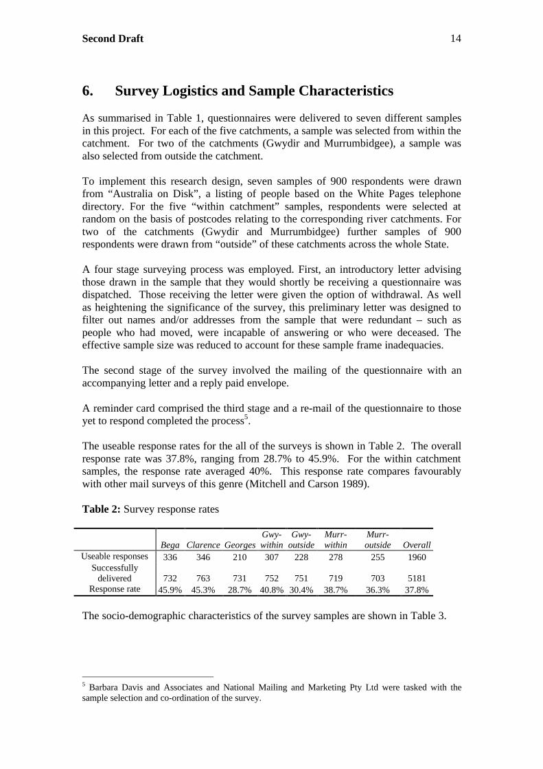
The useable response rates for the all of the surveys is shown in Table 2. The overallresponse rate was 37.8%, ranging from 28.7% to 45.9%. For the within catchmentsamples, the response rate averaged 40%. This response rate compares favourablywith other mail surveys of this genre (Mitchell and Carson 1989).

Table 2: Survey response rates

Bega Clarence GeorgesGwy-within

Gwy-outside

Murr-within

Murr-outside Overall

Useable responses 336 346 210 307 228 278 255 1960Successfully

delivered 732 763 731 752 751 719 703 5181Response rate 45.9% 45.3% 28.7% 40.8% 30.4% 38.7% 36.3% 37.8%

The socio-demographic characteristics of the survey samples are shown in Table 3.

5 Barbara Davis and Associates and National Mailing and Marketing Pty Ltd were tasked with thesample selection and co-ordination of the survey.

Second Draft 15

Table 3: Socio-demographics of the survey samples

Clarence Bega Georges Murr-within

Murr-outside

Gwy-Within

Gwy-outside

Age (yrs) 55.9 52.6 51.1 50.5 52.9 51. 5 52.4Sex (%female) 41% 41% 30% 45% 39% 34% 36%Children 87% 83% 89% 84% 85% 85% 80%

Education# 3.9 4.3 4.1 4.1 4.3 4.1 4.3Income $32,256 $38,899 $46,069 $50,548 $50,251 $43,517 $47,989

# 1-never went to school, 6-tertiary degree

7. Values for the Environmental Attributes of NSWRivers

The objective of this project is to estimate the values of environmental attributes ofrivers. These attribute value estimates will be of use to WMCs in their considerationsof alternative water sharing arrangements. Technically, these estimates (also knownas implicit prices) are appropriate for use in cost-benefit analysis where benefitestimates resulting from incremental changes in river attributes are required.

To estimate these values, the choice data collected in the surveys were analysedstatistically. In essence, the analysis involves searching for relationships between thelevels of the attributes used to describe the outcomes of alternative river managementstrategies and the probability that respondents will choose a strategy. At the sametime, the statistical process used looks for relationships between the choicesrespondents made and their socio-demographic characteristics (eg age, income, sex).

From the relationships between choices made and the levels of the attributes andrespondents’ characteristics identified, attribute values can be estimated. The attributevalues estimated for each of the rivers covered in this study are presented in Tables 4to 8 and in Figures 2 to 6. Technical details of how these estimates are derived areprovided in Appendix C.

Table 4: Vegetation attribute value estimates

River/sampleValue per one percent increase in the length of the river with

healthy native vegetation and wetlands($)

Within catchment sampleBega 2.32Clarence 2.02Georges 1.51Murrumbidgee 1.45Gwydir 1.49Outside catchment sampleMurrumbidgee 2.17Gwydir 2.01

Second Draft 16

Table 5: Fish attribute value estimates

River/sampleValue per unit increase in the number of native fish species

present($)

Within catchment sampleBega 7.37Clarence 0.08*Georges 2.11Murrumbidgee 2.58Gwydir 2.36Outside catchment sampleMurrumbidgee 3.81Gwydir 3.43

* insignificant coefficients in model at the 5 percent level.

Table 6: Waterbird and other fauna attribute value estimates

River/sampleValue per unit of an increase in the number of waterbird and

other fauna species present($)

Within catchment sampleBega 0.92Clarence 1.86Georges 0.67*Murrumbidgee 1.59Gwydir 2.36Outside catchment sampleMurrumbidgee 1.80Gwydir 0.55*

* insignificant coefficients in model at the 5 percent level.

Table 7: Water quality attribute value estimates (1)

River/sampleValue of increasing water quality from boatable to fishable

across the whole river($)


Second Draft 17

Table 8: Water quality attribute value estimates (2)

River/sampleValue of increasing water quality from fishable to swimmable

across the whole river($)


Figure 2: Attribute Value Estimates - Vegetation (within catchment samples)

$0.00

$0.50

$1.00

$1.50

$2.00

$2.50

Bega Clarence Georges Murrum -within

Gwydir -within

Figure 3: Attribute Value Estimates - Vegetation (outside catchment samples)

$1.90

$1.95

$2.00

$2.05

$2.10

$2.15

$2.20

Murrum - outside Gwydir - outside

Second Draft 18

Figure 4: Attribute Value Estimates - Fish species (within catchment samples)

$0.00$1.00$2.00$3.00$4.00$5.00$6.00$7.00$8.00


Gwydir -within

Figure 5: Attribute Value Estimates - Fish species (outside of catchment

samples)

$3.20$3.30$3.40$3.50$3.60$3.70$3.80$3.90


Figure 6: Attribute Value Estimates - Waterbirds and other fauna (within

catchment samples)

$0.00

$0.50

$1.00

$1.50

$2.00


Gwydir -within

Second Draft 19

Figure 7: Attribute Value Estimates - Waterbirds and other fauna (outside of

catchment samples)

$0.00

$0.50

$1.00

$1.50

$2.00


Figure 8: Attribute Value Estimates - Boatable to Fishable (within catchment

samples)

$44.00

$46.00

$48.00

$50.00

$52.00

$54.00


Gwydir -within

Figure 9: Attribute Value Estimates - Boatable to Fishable (outside of

catchment samples)

$28.50

$29.00

$29.50

$30.00

$30.50

$31.00


Second Draft 20

Figure 10: Attribute Value Estimates - Fishable to Swimmable (within

catchment samples)

$0.00$10.00$20.00$30.00$40.00$50.00$60.00$70.00

Beg

a

Cla

renc

e

Geo

rges

Mur

rum

- w

ithin

Gw

ydir

-w

ithin

Figure 11: Attribute Value Estimates - Fishable to Swimmable (outside of

catchment samples)

$0.00$10.00$20.00$30.00$40.00$50.00$60.00$70.00


The reliability and accuracy of the estimates displayed can be judged in a number ofways. First, the strength of the statistical models that underpin the estimates providesa means of assessing the validity of the analysis. The models estimated for this studyare able to explain an exceptionally large proportion of the total variability displayedin the raw data. That is, the models are extremely good at explaining the choicebehaviour of the respondents.

In particular, the attributes used to describe the outcomes of river managementstrategies were consistently found to be significant in determining respondents’choices. Furthermore, the direction of the relationships between attribute levels andchoices were as expected. For instance, it was consistently found that rivermanagement options that were more costly were less frequently chosen byrespondents whilst options providing more species of fish were chosen morefrequently.

Similarly, respondents’ ages, their income and their attitudes to environmental issueshad significant influences on choice behaviour and in directions that are predicted by

Second Draft 21

theory. For instance, respondents with higher incomes were prepared to pay more forenvironmental improvements than respondents with lower income.

A further factor indicating the strength of the value estimates is the high response rateachieved in the surveys. The response rates achieved for the Bega and Clarencesurveys were greater than 45 per cent, a remarkable rate compared to other AustralianCM applications that have used a mail out mail back format. Even the two poorestresponse rate samples (Georges and Gwydir-outside) were well in excess of 25 percent, a rate that is commonly accepted as reasonable for mail questionnaires of thislevel of complexity.

Notwithstanding these indicators of validity, there are numerous factors that need tobe considered when deliberating on the confidence with which the attribute valueestimates can be used. These factors will be discussed in the following sections.

8. Interpreting the Value Estimates

The units of measurement of the attribute value estimates displayed in Tables 4 to 8are dollars per unit of each attribute. For instance, from the Bega River survey, theFish Specie attribute value can be interpreted as:

On average, respondent households in the Bega Valley value the presence of anadditional fish specie in the river at $7.37 per household.

The units used to measure the attributes are different for each attribute. Whilst the fishattribute value is per additional species, the vegetation attribute is per an additionalpercent of the river having healthy riverside vegetation and wetlands. In addition, thewater quality (recreational opportunities) attribute has a different interpretationbecause, unlike the other attributes its unit of measurement was qualitative rather thanquantitative. The water quality attribute is thus broken up into two “levels” –“boatable to fishable” and “fishable to swimmable”. The attribute values associatedwith the first of these levels is the value, on average, that a respondent householdholds for an improvement in the river’s water quality from its current level “suitablefor boating along its length” to the point where it is suitable for fishing along itslength. For instance:

On average, each respondent household in the Clarence River sample values animprovement in river water quality that would make it safe for fishing along thelength of the river at $47.92.

Furthermore:

To have the river water quality improved further so that it would be swimmableacross its length, would be valued (on average) by the Clarence respondents at anadditional $24.46 per household.

The use of qualitative, discrete levels for the water quality attribute requires furtherinterpretation when a change occurs that lies between the defined levels. For example,if a management change causes an improvement in water quality from boatable tofishable from 40 percent of the river’s length to 60 percent of its length, it is necessary

Second Draft 22

to adjust the attribute value estimates because they are predicated on the improvementoccurring over the entire length of the river. The adjustment required necessarilyinvolves an assumption regarding the behaviour of value as less of the river isaffected. The most straightforward assumption that can be made in this regard is thatthe relationship between value and length of the river affected is linear. In otherwords, if an extra 20 percent of the river is affected, the value associated with theimprovement is 20/60 percent (ie 33%) of the value estimate for the whole river6.Using the Gwydir as an example:

On average, each respondent household in the Gwydir River sample values animprovement in river water quality that would make it safe for fishing along 66percent of the river at $25.65.

Because the units of measurement are different across the attributes, the valueestimates for the different attributes are not directly comparable. Hence the valueestimates for the water quality attributes, swimming and fishing, may initially seemcomparatively large. However, the differences may not be so great once differencesin the units of measurement are taken into account.

For instance in some catchments, policy induced changes in the levels of the attributesthat have comparatively small per unit may be substantial. As an example, a 20%increase in the coverage of healthy native riverside vegetation and wetlands mayoccur in some catchments. The relatively small per unit value could thus multiplied bya large amount of attribute change to yield the aggregate value of change. If eachpercent of vegetation coverage increase is estimated to be worth $2.02, as it is for thecase of the Clarence River, then the aggregate value of the increase is $2.02 x 20 =$40.40 per respondent household. On the other hand, the water quality attribute levelsinvolve change across the whole length of the river. The attribute value estimates inthat case represent an already aggregated value of change. Hence consider the case,again of the Clarence, where the value of a river being made fishable rather thanboatable across the whole river was estimated at $47.92. However, the policy underreview may only affect five percent of the river. Thus, the value of the water qualityimprovement would be estimated at $47.92 x .05 = $2.40 per respondent household.

Comparisons are directly possible between the same attributes across different riversand different samples. These results, detailed in Appendix D, indicate that:

• The estimates of attribute values related to the direct use of rivers (swimmingand fishing) tend to be larger for the within catchment respondents than thoseestimated for the comparable outside catchment sample.

• The estimates of values associated more with the ecological condition of therivers (the so-called existence values associated with vegetation, fish and otherfauna) are larger for the samples of respondents living outside the catchmentscompared to the value estimates for the within catchment samples.

• Attribute value estimates generated from within catchment samples arepredominantly different across rivers.

6 Information about the base level of recreational quality in each of the rivers is presented in AppendixI.

Second Draft 23

The implication of these results is that no single set of attribute value estimates can beused as a “source” for the purposes of benefit transfer. Rather, a protocol for thebenefit transfer process will need to be developed to take full advantage of the valueestimation data set generated in this project. Such a protocol is developed in the nextsection.

9. Value Estimates for Benefit Transfer

The attribute value estimates detailed in Section 8 are suited for use in the benefittransfer process. The attribute values held by people living within the catchment ofrivers located in the five regions of the State represented by the five rivers studied inthis report can be estimated with reference to the attribute values provided in Tables 4to 87. For instance, an estimate of the value of an additional 10 percent of healthyvegetation along the Macleay River on the north coast can be “transferred” from theClarence River vegetation attribute value estimate. The exception to this protocol iswhen the attribute value estimates for a representative river are not significantlydifferent from zero. These cases (Clarence/Fish and Georges/Fauna) are aberrationsand require special attention. The approach recommended to deal with the situation isdetailed later in this section.

The transference of “outside” catchment value estimates involves a number ofcomplicating factors most importantly because only two rivers were subjected to“outside” sample CM applications in this study. These were the Murrumbidgee andGwydir Rivers. For these catchments, and in other catchments represented by thesetwo, the “outside” attribute value estimates detailed in Section 8 can be used toindicate an upper bound of the values held by people from outside of the catchment.

For other catchments a different approach is required.

In the case of Sydney urban catchments, the importance of “outside” catchmentvalues is not so significant because of the large number of people living within thatcatchment, and the perception amongst people elsewhere in the state that urban issuesshould be dealt with by the urban populace. Hence, only within catchment valueestimates need be considered.

However, for the northern and southern coastal catchments, where “outside”catchment values are more likely to play a significant role in determining theallocation of water, estimates of such values are required. Again, special attentionneeds to be given to the generation of these “outside” value estimates.

To provide estimates of attribute values where existing within catchment estimates areinsignificant and where relevant outside catchment value estimates are not available, abenefit transfer model has been developed. The model is designed to predict valueestimates on the basis of all the CM data collected from the “within” catchment andthe “outside” catchment samples conducted, excluding the Georges River sample.

7 The values estimated in this report are less reliable as “sources” for “target” rivers located outside thefive regions, most notably the rivers of the far west of the State.

Second Draft 24

This sample has been excluded as it is not relevant for the estimation of “outside”catchment, attribute values for the coastal rivers.

The model allows a significant improvement in the degree of flexibility possible inthe benefit transfer process compared to the straightforward transference of source totarget value estimates. Its use requires the analyst to enter the relevant descriptors ofthe river in question and the sample. The output of the model is a set of attribute valueestimates relevant to the type of river and sample of respondents under consideration.The inputs to the model are:

• Is the catchment in the north or south of the state?• Is the catchment inland or coastal?• Are the respondents whose values are to be estimated living within the

catchment or outside the catchment?

The advantage of using this model is that it allows for transfer across the completearray of catchment/respondent “scenarios”. Specifically, out of catchment valueestimates can be generated for the Bega and Clarence catchments as can estimates forthe insignificant attribute values estimated from the within catchment samples. Themodel is presented in detail in Appendix F.

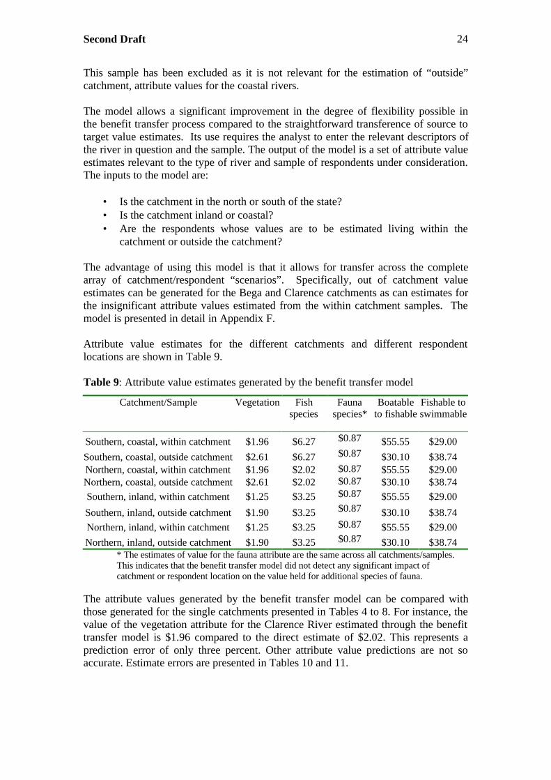
Attribute value estimates for the different catchments and different respondentlocations are shown in Table 9.

Table 9: Attribute value estimates generated by the benefit transfer model

Catchment/Sample Vegetation Fishspecies

Faunaspecies*

Boatableto fishable

Fishable toswimmable

Southern, coastal, within catchment $1.96 $6.27 $0.87 $55.55 $29.00

Southern, coastal, outside catchment $2.61 $6.27 $0.87 $30.10 $38.74Northern, coastal, within catchment $1.96 $2.02 $0.87 $55.55 $29.00Northern, coastal, outside catchment $2.61 $2.02 $0.87 $30.10 $38.74Southern, inland, within catchment $1.25 $3.25 $0.87 $55.55 $29.00

Southern, inland, outside catchment $1.90 $3.25 $0.87 $30.10 $38.74Northern, inland, within catchment $1.25 $3.25 $0.87 $55.55 $29.00

Northern, inland, outside catchment $1.90 $3.25 $0.87 $30.10 $38.74* The estimates of value for the fauna attribute are the same across all catchments/samples.This indicates that the benefit transfer model did not detect any significant impact ofcatchment or respondent location on the value held for additional species of fauna.

The attribute values generated by the benefit transfer model can be compared withthose generated for the single catchments presented in Tables 4 to 8. For instance, thevalue of the vegetation attribute for the Clarence River estimated through the benefittransfer model is $1.96 compared to the direct estimate of $2.02. This represents aprediction error of only three percent. Other attribute value predictions are not soaccurate. Estimate errors are presented in Tables 10 and 11.

Second Draft 25

Table 10: Benefit transfer model estimate errors (%)#: Within catchment samples

Vegetation Fish Fauna Fishable SwimableSouthern coastal/Bega -19 -19 -6 +4 -69Northern coastal/Clarence -3 * -115 +14 +16Southerninland/Murrumbidgee

-16 +21 -83 +4 +30

Northern inland/Gwydir -19 +27 -171 +8 -108# A positive sign on the error indicates that the benefit transfer model overestimates the direct estimate.* Insignificant attribute value estimate at the five percent level.

Table 11: Benefit transfer model estimate errors (%)#: Outside catchment samples

Vegetation Fish Fauna Fishable SwimableSoutherninland/Murrumbidgee

-14 -17 -107 -1 -57

Northern inland/Gwydir -6 -6 * +3 +22# A positive sign on the error indicates that the benefit transfer model overestimates the direct estimate.* Insignificant attribute value estimate at the five percent level.

The inconsistency of the benefit transfer model’s ability to predict the value estimatesgenerated directly from the CM data means that it should only be used where thedirect data are unavailable or inappropriate. This is the case for the values held byoutside catchment people for the attributes of southern and northern coastal rivers andthe fauna attribute of inland northern rivers and for the within catchment values forthe fish attribute in northern coastal rivers. In addition, the fauna attribute valueestimate for the urban rivers would need to be generated from the benefit transfermodel.

The estimates of values held for the environmental attributes of rivers recommendedfor use in five regions of NSW are set out in Tables 12 to 16.

Table 12: Attribute value estimates: southern coastal rivers.

Attribute Value estimate($ per within catchmenthousehold)

Value estimate ($ per outside catchmenthousehold)

Vegetation 2.32 2.61Fish 7.37 6.27Fauna 0.92 0.87Water quality:Fishable 53.16 30.10Water quality:Swimable 50.14 38.74

Second Draft 26

Table 13: Attribute value estimates: northern coastal rivers.

Attribute Value estimate ($ perwithin catchmenthousehold)

Value estimate ($ peroutside catchmenthousehold)


Table 14: Attribute value estimates: southern inland rivers.




Table 15: Attribute value estimates: northern inland rivers.




Table 16: Attribute value estimates: urban (Sydney) rivers.

Attribute Value estimate ($ per withincatchment household)

Vegetation 1.51Fish 2.10Fauna 0.87Water quality: Fishable 48.23Water quality: Swimable 28.28

Second Draft 27

The confidence with which these estimates can be used varies from case to case. Ingeneral, the within catchment estimates can be rated as reliable. More caution must betaken when using the outside catchment estimates. There are two reasons for thelower level of confidence to be placed in the outside catchment estimates. First, theestimates for coastal catchments are based on the benefit transfer model that has beenshown to be imperfect in its predictive capacity. The second reason for the lowerconfidence level centres on the characteristic of non-market value estimates known as“framing”.

Value estimates generated from techniques such as CM are subject to the framingeffect. This means that the values estimated are in part determined by thecircumstances in which the valuation exercise is undertaken.

Of particular concern in the case of the environmental attributes of NSW rivers is theimpact of framing on the outside catchment value estimates. It would be expected thatthe attribute values held by outside catchment residents estimated when only one riverwas being considered for environmental improvement would be greater than if manyrivers were to be improved. This difference in value estimates comes about becauserespondents regard rivers as substitutes for each other and because they have limitedbudgets. With more rivers under consideration, the value on a per river basis can beexpected to be lower.

The implication of the framing issue is that the outside catchment estimates presentedhere should be regarded as maximums because they were determined with only oneriver being considered by respondents. Where multiple river improvementprogrammes are being proposed across the State, the outside catchment values shouldnot be applied in the assessment of all the proposals. A downward adjustment toreflect the framing effect should be made.

To determine the extent of this framing adjustment, a separate but parallel CM studyof the values generated by environmental improvements in rivers across the whole ofthe State. The respondents sampled for this exercise were drawn from the populationof the whole State. Hence, they are most appropriately considered as “outside”catchment responses. The results of “State-wide” study are presented in detail inAppendix H.

The estimates of environmental attribute values of rivers across the State that are heldby NSW residents are set out in Table 17.

Table 17: Attribute value estimates for all rivers in the State

Attribute Value ($ per household)Vegetation 4.23Fish 7.70Fauna 2.37Water quality: fishable 44.05Water quality: swimable 87.17

Second Draft 28

The results demonstrate that the attribute value estimates for the whole of the state arelarger than the outside catchment values estimates on a per catchment basis. However,it is clear that if the single catchment value estimates were used for a number ofconcurrent river improvement projects, the State-wide value estimates would beexceeded. Using the single catchment estimates for outside catchment values wouldcause an over statement of environmental improvement benefits.

The implication of these results is that outside catchment estimates for specific riverscan be generated by dividing these State-wide estimates by the number of rivers thatare to be improved at the time. This strategy would ensure that outside values wouldbe estimated conservatively.

10. Issues of Aggregation

The attribute value estimates provided by the individual catchment CM applicationsand the benefit transfer models can be used in the process of calculating estimates ofthe total value society gains from improvements in the environmental conditions ofrivers across the state. However, to generate such estimates of aggregate value, aprocess of extrapolation must be applied.

First, it should be noted that the attribute values estimated in this project do notrequire aggregation over time. They were estimated as one-off payments made byhouseholds and as such represent respondents’ “present values” of the stream of valuethey will enjoy from the attributes through time.

The “within” catchment value estimates can be extrapolated to the catchmentpopulation with reference to the number of households, given that the value estimateswere generated on a per respondent household basis. As a conservative measure, theextrapolation should be made across 38% of the households. This is to account for theresponse rate achieved for the survey. Alternatively, the response rates achieved ineach of the individual surveys could be used for the related rivers.

The practice of extrapolating the value estimates to the proportion of the populationthat responded to the survey is consistent with Boyle and Bishop (1987) who assumedthat non-respondents have a willingness to pay equal to zero. Their rationale for thisassumption is that by not answering the survey, respondents have implicitly indicatedtheir willingness to pay. The problem with this approach is that the reasons peoplehave not responding are varied and not necessarily indicative of a zero value for thegood in question. For instance, some respondents may be unwell or away at the timeof the survey. They may simply be too busy to take the required time out to completethe questionnaire. It is difficult, therefore, to gauge what proportion of non-respondents do have positive values without a comprehensive ex post survey of non-respondents. An alternative to the Boyle and Bishop approach is to use the methodsuggested by Morrison (2000). In a study that involved the estimation of valuesderived from environmental improvements to wetlands, Morrison found thatpotentially, about one-third of non-respondents have value estimates similar torespondents. For the current analysis, this would imply that the appropriate proportionof the population across which extrapolation could be made is 38 per cent plus onethird of the 62 per cent non-respondents: that is 59 per cent. Clearly, this is a lessconservative approach to the estimation of aggregate values.

Second Draft 29

Consider now an example of the aggregation process. Suppose that a rivermanagement option under consideration in a catchment on the south coast wouldincrease the vegetation attribute by five percent, ensure the reintroduction of two fishspecies and improve the water quality across 15 percent of the length of the river fromboatable to fishable. If the catchment had a household population of 4,000 then theappropriate calculation (based on the value estimates set out in Table 11) is:

Within catchment aggregate value estimate = 4000 x 0.38 [ 5 x 2.32 + 2 x 7.37 + 0.15 x 53.16]

= $52,157

Given a NSW population of approximately 1.8m households, the appropriateaggregation calculation for outside catchment values is:

Outside catchment aggregate value estimate = 1.8m x 0.38 [ 5 x 2.61 + 2 x 6.27+ 0.15 x 30.10]

= $20.59m

The total value to all the people of NSW of the improved river environment providedby the proposed management option is therefore in the order of $21m.

It is important to note that the aggregate value reported above is rounded to thenearest $10,000. This is done to avoid impressions of spurious accuracy.

This process can be used for NSW rivers that are located within the regionsrepresented by the five rivers specifically considered in this report.

The relative magnitudes of the “within” and “outside” catchment aggregate valueestimates provides a graphic illustration of the importance of the values enjoyed bypeople who live at a distance from the river. It also underlines the importance ofensuring that potential framing effects caused by the simultaneous assessment ofmultiple rivers are taken into account when estimating outside catchment values.

The aggregation process outlined in this section is subject to a particular limitation. Itinvolves the aggregation of the estimates of individual attribute values. Theoretically,these values are estimates of what respondents are willing to pay to see them increaseby one unit, given that no other changes occur simultaneously. Hence, to use them inthe context of changes across a number of attributes can theoretically causeinaccuracy.

The more appropriate way to estimate the benefits of changes that involve multipleattributes is to use a more complete model of respondent choice behaviour. Thisinvolves the calculation of the benefits people receive from the environmentalcondition of rivers both before and after the change in water management that is beingproposed. Technically, this value is called the Compensating Surplus of the proposedchange. The complete model of choice (detailed in Appendix C, notably Table C2) isused to perform these calculations. A spreadsheet has been devised to perform thesecalculations. It is displayed in Appendix G.

Second Draft 30

The spreadsheet also enables the calculation of aggregated attribute values. Thisaffords a comparison of the two approaches. Value estimates for environmentalimprovements defined by the mid-range levels used in the construction of thealternative options in the choice sets are provided in Table 18. A clear trend emergesfrom the comparison. In all cases, the aggregate values estimated using the attributeapproach are greater than their compensating surplus counterparts. In most cases theextent of the difference is significant.

Table 18: Value estimates for multiple attribute changes (within catchment samples)

ProposedChange

AggregationTechnique

Bega($)

Clarence($)

Georges($)

Gwydir($)

Murrum-bidgee($)

AggregateAttributes

189.10 122.37 125.97 152.64 145.59To midrangelevelsfrom thechoice sets

CompensatingSurplus

66.82 9.71 51.60 142.83 95.60

The difference between the estimates provided by the two approaches is explained bythe fundamental differences that underpin their calculation. The aggregate attributeapproach ignores the overall picture that encompasses the proposed change. Forinstance, the impact of factors other than the specifics of a single attribute change areomitted from the calculation. In contrast, the compensating surplus calculationincorporates the impacts of the numerous factors that influence respondents’ values.One factor that is incorporated in the compensating surplus calculation but omittedfrom the aggregate attribute approach is the propensity for respondents to rejectchange for reasons that go beyond the extent of the attribute change that is offered.For instance, respondents may simply reject change because they are inherentlyconservative. Such motivations are clearly important when large-scale changes areinvolved (such as those which are depicted in Table 18). However, where theproposed changes are marginal, such motives are likely to be irrelevant. The danger ofusing the compensating surplus measure in such cases is to grossly underestimate thevalue of the proposed change. Similarly, the danger of using the aggregate attributeapproach for more substantial changes (as in Table 18) is one of overestimation.

It is therefore recommended that:

• for proposed changes which involve multiple attributes varying by less than 25per cent, the aggregate attribute value should be used; and,

• for multiple attribute changes where larger variation is expected, thecompensating surplus value should be used.

Because most river improvement projects will involve only marginal changes (lessthan 25 per cent increases in attributes) the aggregate attribute approach is likely to bemost frequently employed.

Second Draft 31

11. Conclusion

This report has presented value estimates for the environmental attributes of NSWrivers. The value estimates have been developed specifically for use by the State’sWater Management Committees in their economic analyses of alternative watersharing arrangements as part of the Water Reform Process. The estimates provideinformation on the “non-marketed” values that are generated by rivers. They thereforesupplement information on marketed values provided by rivers such as farmproduction in any analysis of the trade-offs involved in alternative water sharingarrangements.

Specifically five “representative” rivers were selected for detailed analysis using theChoice Modelling technique. These rivers were the Bega, Clarence, Georges, Gwydirand Murrumbidgee. Values for four environmental attributes were estimated. Two ofthese attributes related to biodiversity values: number of fish species and water birdsand other fauna present. Another attribute related to the condition and extent ofriverside vegetation and wetlands. The fourth attribute used recreational activitysuitability as a surrogate for water quality.

Values for these attributes were estimated for samples of households located in thecatchments. For two of the rivers, the Murrumbidgee and Gwydir, samples ofhouseholds resident outside the catchment were also targeted.

A process of benefit transfer has been developed to allow the values estimated for thefive specific rivers – for both within and outside catchment respondents – to be“transferred” for use in the assessment of water sharing arrangements in othercatchments across the state. The protocol designed for this process involves therecognition of regional differences between rivers as well as socio-economicdiversity.

In addition, methods for calculating estimates of aggregated values are described. Inthe first instance, this involves the estimation of values aggregated across multipleattribute changes arising from a single alternative river management proposal on a perrespondent basis. Secondly, the aggregation process involves the extrapolation of theper respondent value estimates to the wider population. The multiple attribute changeaggregation can be carried out in two different ways, depending on the magnitude ofthe changes involved. The extrapolation to the broader community must involve anassumption regarding the extent to which values are held amongst non-respondenthouseholds.

The findings of this study represent a major advance in the provision of informationrelevant to natural resource decision making. Before mechanisms can be put in placeto allocate resources, there is a need to define the outcomes that are desirable forsociety. It is only with a good understanding of both the biophysical relationshipsinvolved and the values that people place on alternatives (as expressed both in andoutside the market) that these outcomes will become known with any confidence.

Second Draft 32

Bibliography

Bennett J. and R. Blamey (2001). The Choice Modelling Approach to EnvironmentalValuation, Edward Elgar, Cheltenham.

Bennett, J., M. Morrison and R. Harvey (2000). A River Somewhere – Valuing theEnvironmental Attributes of Rivers. Paper presented at the ISEE 2000 Conference,ANU Canberra , 5-8 July.

Boyle, K.J. and Bishop, R.C. (1987). Valuing Wildlife in Benefit-Cost Analyses: A

Case Study Involving Endangered Species. Water Resources Research, 23(5): 943-

950.

Desvousges, W.H., Naughton, M.C. and Parsons, G.R. (1992). Benefit Transfer:Conceptual Problems in Estimating Water Quality Benefits Using Existing Studies.Water Resources Research, 28(3): 675-683.

Department of Land and Water Conservation (1998). Water Sharing in New SouthWales – access and use. DLWC Discussion Paper, Sydney.

Hausman, J.A. and Ruud, P. (1987). Specifying and Testing Econometric Models forRank-Ordered Data. Journal of Econometrics, 34: 83-10.

Kling, C.L. and C.J. Thomson (1996) The Implications of Model Specification forWelfare Estimation in Nested Logit Models, American Journal of AgriculturalEconomics, 78, pp. 103-114.

Lockwood, M. and Carberry, D. (1998). Stated Preference Surveys of RemnantVegetation Conservation. Report No.104, The Johnstone Centre, Charles SturtUniversity.

Morrison, M. (2000). Aggregation Biases in Stated Preference Studies.Australian Economic Papers, 39(2): 215-230.

Morrison, M.D. and Bennett, J.W. (2000). Choice Modelling, Non-use Values andBenefit Transfer. Journal of Economic Analysis and Policy, 30(1): 13-32.

Morrison, M., Bennett, J. and Blamey, R. (1999). Valuing Improved Wetland QualityUsing Choice Modelling. Water Resources Research. 35(9): 2805-2814.

Poe, G.L., Severance-Lossin, E.K. and Welsh, M.P. (1994). Measuring the Difference(X-Y) of Simulated Distributions: A Convolutions Approach. American Journal ofAgricultural Economics, 76: 904-915.

Rolfe, J.C., Bennett, J. W and Louviere, J. J 2000, Choice Modelling and its PotentialApplication to Tropical Rainforest Preservation, Ecological Economics, Vol. 35, pp.289-302.

Second Draft 33

Van Bueren, M. and Bennett, J. W. 2000, Estimating Community Values for Land andWater Degradation Impacts, draft report prepared for the National Land & WaterResources Audit Project, Unisearch Pty Ltd, Canberra.

Second Draft 34

Appendix A Attribute Determination

One of the key tasks involved in undertaking CM applications is determining whichattributes should be used to depict the environmental outcomes of alternative watermanagement strategies. It is important because unless the natural resource that isbeing valued can be decomposed into a parsimonious and meaningful set of attributes,then the validity and usefulness of the estimates could be compromised. While thismay seem to be a straightforward task, it is arguably one of the most difficult andcritical task in any environmental choice modelling application. Moreover, it is alsonecessary to select levels for attributes. This can also be very challenging. Formarketed consumer goods and services, levels are usually readily defined. But this isnot the case in environmental applications. For example, consider all of the differentways that water quality is measured. Which one should be used? Which one wouldbe most meaningful for the general public?

In this appendix, the process used to determine these attributes and select the attributelevels is set out. A three-stage process was used to select attributes and the appendixis structured to reflect those stages. In section A.1, a review of the existing literatureundertaken to determine the attributes previously used in studies seeking to valueimproved water quality or river health using choice modelling or similar approaches isoutlined.

Next, “supply-side” determinants of attributes are discussed. These factors reflect therequirements of those conducting the research and those who will use the results ofthe CM applications. From this perspective, attributes must be defined to be useful inthe policy determination process. Hence, they must be consistent with theenvironmental variables scientists are able to predict will change when watermanagement strategies change, and for which scientific information is available. Thelink between management strategy and community value has to be maintainedthrough the selection of attributes.

In section A.3 of the appendix, the “demand-side” influences on attribute selection arediscussed. These factors relate to the requirements of the CM questionnairerespondents. The environmental outcomes described to respondents in a CMapplication must be meaningful to them. Environmental attributes that are outside theexperience of respondents are therefore unlikely to encourage reliable responses.Again, the selection of attributes that are relevant to respondents maintains the linkagebetween management strategy and community value.

In sectionA.4, the strategy used to select attribute descriptors once the set of attributeshad been determined is discussed. The appendix concludes with a discussion of theuse of the set of attributes finally determined.

A.1 Previous research

In the first instance, some information on appropriate attributes, from the analyst’sperspective, can be gleaned from the work of others.

Several previous studies have examined the value of improving the quality of rivers.The earliest of these, CVM applications by Whitmore and Cavadias (1974) and Smith

Second Draft 35

and Desvousges (1986) did not seek to isolate attributes for the different aspects ofimproved river quality. Rather, they used what has been described as a ‘water qualityladder’ to represent changes in the quality of the river. In the Whitmore and Cavadias(1974) study there were five levels to the ladder:

(1) no-life,(2) the present (ie current situation),(3) swimming,(4) drinking; and,(5) natural.

In the Smith and Desvousges (1986) study, there were also five levels:

(1) worst possible water quality,(2) okay for boating,(3) gamefish like bass can live in it,(4) safe for swimming; and,(5) safe to drink.

These water quality ladders were used as a means of simplifying the communicationof changes in water quality to respondents. However, it is only possible to use theresults of these studies to value changes in these discrete quality levels.

In a more recent study that used conjoint analysis techniques, ACIL Economics andAGB McNair (1996) used a set of five environmental attributes (in addition to a set ofmanagement attributes). These attributes were:

(1) risk of algal bloom,(2) number of unsafe swimming days,(3) effects on fish stocks,(4) need for treatment of water for drinking; and,(5) effects on the catchment ecosystem.

Each of these attributes was not described quantitatively. Rather qualitativedescriptors such as ‘unchanged’, ‘slightly increased’ and ‘moderately increased’ wereused.

Garrod and Willis (1998) conducted a slightly different study using CM. Theirobjective was to estimate the loss of amenity value for inland waterways caused bypublic utilities. They, therefore, included three public utility attributes in theirquestionnaires instead of environmental outcomes. The utilities involved were pipebridges, pylons and cable crossings. Each of these attributes was described in termsof percentage reductions.

The Centre for International Economics (1997) focused on the community’swillingness to pay for various water supply options in the Australian Capital Territoryin their CM application. Several attributes relating to river quality were included.These were ‘environmental flows’ and ‘habitat loss’. The first attribute was describedaccording to whether there would be improvements in flow in no, some or all rivers.The second attribute was quantitative, with habitat loss occurring for between zero

Second Draft 36

and 10 species.

Griner (1997) conducted a further study that used conjoint analysis. Specifically,conjoint ranking was used to value improved river quality. The only environmentalattribute used was “river health” and that was described as being either “unpolluted”,“moderatley polluted” or “severely polluted”.

In summary, the literature provides few guidelines for the definition of attributes todescribe the environmental quality of rivers. Apart from the ACIL Economics andAGB McNair (1996) study, none of the studies reviewed attempted to disaggregateriver quality into its component attributes. This dearth of evidence places even moreimportance on other approaches to determining attributes.

A.2 Supply-side Determinants

After the literature review was conducted, a sample of policy makers and researcherswere surveyed to determine, from a management perspective, what attributes theythought should be used to describe river health. Twenty three respondents8, werecontacted by email and asked a short sequence of questions:

“Q1: Please indicate up to 10 environmental attributes/characteristics thatcan be used as indicators of river health. Bear in mind that these attributesmust be readily understood by members of the general public.

Q2: Please indicate on what basis you made your selection. In other words,why are the attributes/characteristics you chose appropriate indicators ofriver health?

Q3: If you were limited to only choosing five out of the 10 attributes, whatwould they be? Why?”

The attributes suggested by respondents in the survey included:

• Flow (natural flow, degree of regulation)• Fish (native fish population, species diversity)• Vegetation (riparian, wetland, floodplain, aquatic)• Exotics (carp, willows, gumbosia, weeds)• Channel condition (bank erosion, sediments)• Waterbirds• Water quality (algal blooms, salinity, turbidity, nutrients, pesticides,

coliforms)• Water dependent fauna (macroinvertibrates, stream fauna, eg frogs and

platypus, aquatic biodiversity)• Recreational use• Visual amenity

8 Respondents were drawn from the various state government departments that are involved in thewater reforms process (eg, Agriculture, Forestry, Land and Water Conservation, Fisheries and theEPA), non-government conservation organisations and community representatives. The respondentsincluded people with both research and policy backgrounds.

Second Draft 37

The five attributes that were mentioned most frequently by the respondents were:

• Flow• Fish (including exotics)• Vegetation (including wetland and channel condition)• Water quality• Water dependent fauna

A feature of the approach taken to the supply-side definition was an attempt to temperthe responses of the research/ policy stakeholders by asking them to provide attributesthat would be “readily understood by members of the general public”. In this way, thefirst step was taken to reconciling any possible divergence between the supply anddemand sides of the attribute definition task.

Furthermore, the attributes discovered using the supply-side approach, were testedduring the demand-side phase, which is discussed in the following section.

A.3 Demand-side determinants

While policy concerns can influence which attributes are included in choice sets, it isunwise to include attributes that are only relevant from a policy perspective and notrelevant to respondents. This is because they will probably be ignored by respondentsand hence will be insignificant explanatory variables. However, some attributes ofmarginal relevance to respondents, but important for policy, could be included.

Focus groups are a useful means of identifying attributes that are relevant forrespondents. It provides the opportunity to ask respondents directly or indirectlywhich attributes they think are most relevant.

One approach to identifying relevant attributes in focus groups was described byMorrison, Bennett and Blamey (1997). Respondents were told that there were twodifferent options for the improvement in the quality of a wetland. They were thenasked what information they would like to know if they were to choose between theoptions. The strength of this approach is that participants are placed in a position ofchoice when they are identifying relevant information. The weakness was that theytended to identify large amounts of information, which had to be distilled by theresearchers.

There are several alternatives to the approach used by Morrison et al (1997). Onealternative is to augment their procedure. First, respondents can be asked to identifyall relevant attributes or characteristics of rivers that are relevant to them in makingtheir choices. If a large number are identified, respondents can be asked whichattributes they would want to know about if they could only be told about a few ofthem.

An alternative is to start with a list of the attributes identified by the survey ofresearch/policy stakeholders. Respondents can be asked to add any other attributesthat they consider important to this list. Then, similar to the previous approach,respondents can be asked which attributes they would want to know about if they

Second Draft 38

could only be told about a few.

Both of these approaches were used in a sequence of four focus groups that were heldbetween June and August 1999 to determine river environment attributes from ademand side perspective. Two of the focus groups were held in Sydney and theremaining two were held in the regional centres of Yass and Wagga Wagga9.Professional marketing research firms were used to recruit the participants for two ofthe focus groups10. The participants for the remaining groups were recruited usingcommunity contacts in Sydney and in Yass.

Prospective participants for the groups were told that they would be attending adiscussion about an “issue of community concern”. Recruitment was designed toensure an even distribution of ages and an approximately equal balance between menand women. The authors of this report moderated the focus groups meetings11. All ofthe meetings were recorded using audio-tapes.

The focus group participants were initially asked several questions about their beliefsregarding the condition of rivers, and what action is being taken to reduce theseproblems.

After the issue of river health had been sufficiently introduced and respondents weremade aware of the purpose of the focus group, they were then asked the followingquestion:

“Suppose that the government was considering two different options forimproving the quality or health of the Murrumbidgee River (or one of theother rivers previously mentioned). Suppose also that you were asked whichof these two alternatives you preferred. If you could ask for information aboutchanges in any of the characteristics or attributes of the river, what would youwant to know?”

Various river characteristics emerged from the discussions that arose in the twogroups, including the following:

• flow• healthy vegetation• fish• waterbirds• clean water• non-eroded banks• healthy ecosystem• habitat• balance amongst water users

9 The Sydney groups were held on Monday 21 June and Wednesday June 30, the Yass group was heldon Tuesday 15 June, and the Wagga Wagga group was held on Friday 17 August.10 Applecorn Research recruited the participants to the first Sydney focus group, and Art ProfessionalMarketing recruited the participants to the Wagga Wagga focus group.11 The assistance of Stuart Whitten in moderating the Wagga Wagga focus group is gratefullyacknowledged.

Second Draft 39

• recreational quality

Because the number of attributes in a CM choice set has to be limited to a number thatis within the cognitive limits of most respondents, this list had to be prioritised. If toomany attributes are used to describe environmental outcomes, respondents may seekto simplify the exercise by using heuristics (Mazotta and Opaluch 1995, Swait andAdamowicz 1996). Alternatively, they may choose not to complete the questionnaireat all if the outcome descriptions become too complex because of the number ofattributes included. According to Carson, Louviere, Anderson, Arabie, Bunch,Hensher, Johnson, Kuhfeld, Steinberg, Swait, Timmermans and Wiley (1994) theaverage questionnaire includes about seven attributes. In the context of riverenvironments, respondents typically know much less about the good involved andmay find a questionnaire difficult to answer if seven or more attributes are included.Hence the use of fewer attributes may be appropriate.

The focus group participants were asked the following question to reduce the numberof attributes to be used to describe the environmental outcomes:

“Suppose that from this list of attributes/characteristics that have just beengenerated you could only receive information about five of them. Which fivewould you want to know about (in order of priority)?”

Respondents were asked to write down their answers on a sheet of paper. The topfour rankings given to each of the attributes in the two groups are summarised inTable 1.

It is evident from Table A.1, that water quality is the most important attribute torespondents in both focus groups. Both vegetation and wildlife (including bothwaterbirds and fish) were consistently important to participants in both focus groups.Flow tended to be more important to participants in the Sydney focus group, whilerecreational quality was a more important characteristic to participants in the Yassfocus group.

These attributes closely parallel those found in the survey of policy advisers andresearchers detailed in the previous section of this paper. In that stakeholder surveythe five main attributes that emerged were flow, fish, vegetation, water quality andwater dependent fauna.

The convergence between the attributes suggested by stakeholders and members ofthe community, as represented by the focus group participants, provides usefulevidence that the attributes emerging will be both useful to policy makers and relevantto CM questionnaire respondents.

Second Draft 40

Table A.1: Rankings of attribute importance*

Attributes R1(Y) R2(Y) R3(Y) R4(Y) R1(S) R2(S) R3(S) R4(S)

Clean Water 5 2 1 - 2 4 - 2Vegetation - 3 2 4 - 4 1 3

Wildlife(birds/fish)

- 2 3 - - 1 1 -

Water birds 1 - 1 1 - - - 1Fish - - 2 - 1 - 4 -

Flow 1 - - - 5 - 1 -

RecreationQuality

1 3 - 3 - - - -

* R1 (Y) represents a ranking of 1 (the highest ranking) for the Yass group. Correspondingly, R1(S)represents the highest ranking of the Sydney group. Hence, in the Yass focus group, five participantsranked “clean water” as the most important attribute, whilst in the Sydney group five participantsranked “flow” as the first priority

However, one problem remains with this list of attributes. This relates to the existenceof causality amongst attributes. Some relevant environmental attributes may beperceived by respondents to be causally prior to other environmental attributes. Forexample, a change in water quality in a wetland may be believed by respondents tocause a change in the number of waterbirds breeding. If respondents have this belief,they may focus on the ‘indicator’ attribute and discount information about the otherattributes12. The inclusion of an ‘indicator’ or causally prior attribute may make otherattributes redundant. Hence it may be desirable to include either the indicator or theother attributes, but not both. The omission of attributes that focus group participantshave identified as being of significance can however other impacts. Respondents maybe frustrated that an attribute they believe should be detailed is not included. Theplausibility of the CM questionnaire may therefore be cast into doubt.

The attribute that the focus group participants considered most important (waterquality) is potentially an indicator attribute. To some extent this problem can beaddressed through the way attributes are defined for respondents.

A.4 Selection of Attribute Descriptors

After the attributes have been selected, it is necessary to select ways to describe eachof these attributes. In CM applications it is possible to use both qualitative andquantitative descriptors of the attributes, however the latter are preferred for the rivervaluation exercise because they are more useful for benefit transfer. This is becausethey can be measured in a more objective fashion across different river systems. 12 A test of the effect of causal attributes was reported in Blamey, Rolfe, Bennett and Morrison (1997).The authors found some support for the hypothesis that the inclusion of a causal heuristic can affectrespondents’ choices.

Second Draft 41

Attempts were initially made to select suitable levels by questioning respondents. Inthe Yass focus group, participants were asked the following question:

“So far we have identified a number of characteristics or attributes of rivers. Wewould also like to identify different ways of describing these characteristics. Forthe following characteristics (flow, fish, vegetation, water quality and waterdependent fauna) could you list all of the different ways that you can think ofdescribing them?”

Participants generally had difficulty in suggesting suitable descriptors for theattributes but they were able to suggest the key words and phrases set out in TableA.2:

Table A.2: Attribute key words and phrases.

Flow:• natural flow• following seasons, rainfall events

Fish:• number of different species• no carp• healthy

Vegetation:• native• healthy• no noxious weeds

Water quality:• drinkable• blue green algae• clear• no smell

Water dependent fauna:• existence of native fauna (platypus,

frogs, turtles)• diversity

Based on the information gathered from this focus group, the information derivedfrom the literature review and the information previously provided through the surveyof policy makers and researchers, a list of different alternatives was developed. Thislist was used as the basis of a discussion amongst the participants in the first Sydneyfocus group. That list of alternatives is shown in Table A.3.

For the flow attribute, Options 2 and 3 received the most support from focus groupparticipants. For the fish attribute, participants preferred Options 2 and 4.Participants wanted the number of native fish species present to be described, but theyalso liked having the health of the species being described. For vegetation, Option 2was the clear favourite. One participant suggested that a percentage rather than actualarea be used as the descriptor.

Second Draft 42

Table A.3: Alternative attribute descriptors

Attribute DescriptorFlow:Option 1 Percentage of natural flowOption 2 Percentage of average natural flowOption 3 Percentage of average natural flow/ Large summer and low winter

flowsOption 4 No change, moderate increase, large increase

Fish:Option 1 Percentage of native fish species presentOption 2 Number of native fish presentOption 3 Number of native fish species presentOption 4 Percentage of native fish present/Health of species (poor, fair,

good)

Vegetation:Option 1 Area of wetlands and riverside vegetationOption 2 Area of healthy wetlands and riverside vegetationOption 3 Poor condition, moderate health, healthy

Water Quality:Option 1 Worst possible quality, OK for boating, OK for fishing, OK for

swimmingOption 2 Unpolluted, moderately polluted, severely pollutedOption 3 Mostly poor, sometimes OK, Mostly goodOption 4 Number of unsafe swimming days paOption 5 Number of days pa affected by algal blooms

Wildlife:Option 1 Native species present along the riverOption 2 Number of water bird and other native species along the riverOption 3 Water bird species presentOption 4 Threatened and non-threatened species present

Of particular note is the treatment of the water quality attribute. The approach takenwas to channel participants’ interest in water quality toward its impacts specifically onrecreation opportunities. In this way, the causality of the attribute was diffused.Option 1 received the greatest support. This was because of its relevance to thepublic. Hence, the strategy of using this descriptor demonstrated that problems withindicator attributes may be minimised or avoided. To enhance this effect, the attributewas re-named “recreation use”.

Finally, for the wildlife attribute, Option 2 clearly received the greatest support.

Except for flow, these attribute and their descriptors were selected as the mostappropriate for use in the choice modelling applications for the water reform process.Flow was excluded as an attribute for parsimony, and because it was thought that flowwas a management strategy rather than an outcome attribute. Because it would be one

Second Draft 43

of the main factors causing the changes in the environmental attributes, the difficultiesof attribute causality would again have been apparent.

A.5 Conclusions

A critical issue in any environmental choice modelling application is the selection ofattributes and respective levels. It is critical because it determines the usefulness andvalidity of the resulting estimates. The selection of attributes for environmentalvaluation purposes is far more difficult than for applications involving marketedconsumer good. In the latter, the attributes of a good are far more apparent. In anenvironmental choice modelling application it is necessary to consult both the endusers of the value estimates so obtained and the community.

A three-stage process was used to select attributes for the water reform process choicemodelling application detailed here. First a literature review was conducted, secondmanagers and researchers were surveyed, and finally a series of four focus groups wascompleted. Five attributes were selected through this process: flow, fish, vegetation,water quality and wildlife. A noteworthy finding was the convergence in viewsamongst managers and researchers and the community. However, some issues stillremained for the selection of attributes, particularly how to resolve the perceived (andactual) causality amongst attributes. This necessitated the exclusion of one of theattributes (flow) and the use of recreational characteristics to proxy for water quality.

The methodology used to select attribute levels has also been discussed. Similar tothe selection of attributes, this is again arguably more challenging in theenvironmental valuation case than for marketed consumer goods and services. Theapproach of asking focus group participants to suggest indicators was initially trialed.However, this task was met with some difficulty. The approach used in later focusgroups, of showing participants sets of alternative descriptors and asking them tonominate their preferred alternatives or make suggestions, was more effective.

APPENDIX BIBLIOGRAPHY

ACIL Economics and AGB McNair (1996). A Framework for Assessing CommunityDemand for Water Quality Values. Report prepared for the NSW EnvironmentProtection Authority, ACIL, Sydney.

Blamey, R.K., Rolfe, J.C., Bennett, J.W. and Morrison, M.D. (1997). EnvironmentalChoice Modelling: Issues and Qualitative Insights. Research Report No.4. School ofEconomics and Management, University College, The University of New SouthWales.

Carson, R.T., Louviere, J.J., Anderson, D.A., Arabie, P., Bunch, D.S., Hensher, D.A.,Johnson, R.M., Kuhfeld, W.F., Steinberg, D., Swait, J., Timmermans, H. and Wiley,J.B. (1994). “Experimental Analysis of Choice”. Marketing Letters, 5(4): 351-368.

Second Draft 44

Centre for International Economics (1997). A Study to Assess Environmental ValuesAssociated With Water Supply Options. Final Report Prepared for ACTEWCorporation, Canberra.

Garrod, G. and Willis, K. (1998). “Using Contingent Ranking to Estimate the Loss ofAmenity Value for Inland Waterways from Public Utility Service Structures”.Environmental and Resource Economics, 12: 241-247.

Griner, B. (1997). Valuing Watershed Quality Improvements Using Conjoint Analysis.Unpublished Paper, Graduate School of Public and International Affairs, Universityof Pittsburgh.

Mazzotta, M.J. and Opaluch, J.J. (1995). “Decision Making When Choices AreComplex: A Test of Heiner’s Hypothesis”. Land Economics, 71(4): 500-515.

Morrison, M.D., Bennett, J.W. and Blamey, R.K. (1997). Designing ChoiceModelling Questionnaire Using Focus Groups: Results from the Macquarie Marshesand Gwydir Wetlands Cast Studies. Choice Modelling Research Report No.5. Schoolof Economics and Management, The University of New South Wales.

Smith, V.K. and Desvousges, W.H. (1986). Measuring Water Quality Benefits.Kluwer-Nojhoff Publishing, Boston.

Swait, J. and Adamowicz, W. (1996). The Effect of Choice Environment and TaskDemands on Consumer Behaviour: Discriminating Between Contribution andConfusion. Unpublished Working Paper, Department of Marketing, University ofFlorida.

Whitmore, G.A. and Cavadias, G.S. (1974). “Experimental Determination ofCommunity Preferences for Water Quality-Cost Alternatives”. Decision Sciences,5:614-631.

Second Draft 45

Appendix B: Sample Questionnaire

Second Draft 46

Second Draft 47

Second Draft 48

Second Draft 49

Second Draft 50

Second Draft 51

Second Draft 52

Second Draft 53

Second Draft 54

Second Draft 55

Second Draft 56

Second Draft 57

Second Draft 58

Second Draft 59

Second Draft 60

Appendix C Modelling results

Each of the data sets were analysed using a nested logit model. In the nested logitmodel unobserved components of utility are assumed to be shared between certainalternatives. Hence the errors of the alternatives are correlated and not independent.This form of model is used to avoid problems associated with potential violations ofthe required condition that alternatives be independent and irrelevant.

When using nested logit models a ‘tree-structure’ is pre-specified. Tree structuresreflect the existence of homogenous sets of alternatives that have correlated errors.They can have multiple levels. All of the alternatives are in the branches at thebottom of the structure. These alternatives are then grouped at the next level using thelimbs of the tree. The tree effectively represents the choice process used byrespondents when deciding between alternatives. Hence, it is assumed thatrespondents first decide if they want to support any change in river management (iethey choose between Option A, the status quo, and the other options). Subsequently, ifthey have not selected the status quo then they are assumed to choose between the“change” alternatives on the basis of their attributes .

Following Kling and Thompson (1996), the nested logit model can be specified asfollows. The probability of a particular alternative being chosen (Pjm) is equal to theprobability that the limb that the alternative is in is chosen (P(m)) multiplied theprobability that the alternative is chosen from within the limb P(j|m). That is:

Pjm = P(j|m).P(m)

where:

In the above equation, Im is the inclusive value and is the sum of the utility of all ofthe alternatives. The model works by estimating the probability that an alternative ischosen within a limb P(j|m) and estimating the probability that a limb is chosen(P(m)).

The coefficients estimated using the nested logit model are used to derive estimates ofthe value of an environmental improvement. The focus of this report is on theestimation of implicit prices. These are point estimates of the value of a unit changein an attribute. They are useful for management decisions where information isrequired about the value of marginal changes in environmental quality, such as the

α=

α

α=

α=

∑

∑

=

=

mJ

1imimm

M

1kkk

mm

m

mjm

)/Vexp(logI

)Iexp(

)Iexp()m(P

)Iexp(

)|Vexp()m|j(P

Second Draft 61

value of an extra waterbird specie preserved. They are also useful for identifying therelative importance people place on different attributes.

Attribute values (implicit prices) are calculated as follows, where utility is a linearfunction of all attributes:

IP = βA/βM

where IP is the implicit price, βA represents the coefficient of the Ath non-monetary attribute, and βM represents the coefficient of the monetary attribute.

The variables used in the nested logit models, and their expected signs, are presentedin Table C.1. Note that for the socio-demographic variables, the expected signs areopposite to what would normally be expected as these variables have been interactedwith the constant representing the continuation of the current situation option.

Table C.1: Variables used in the nested logit models

Variable Definition Expected signASC1, 2 Alternative Specific Constants ?*RATE Increase in water rates −VEGET % healthy native riverside vegetation +FISHSPEC Number of native species present +FISHING1 Suitable for fishing +SWIMMING Suitable for swimming +FAUNA Number of waterbirds and other fauna

present+

PROGRE Progreen environmental orientation −PRODEV Prodevelopment environmental orientation +AGE Age (years) +INCOME Income ($) −INCDUM Dummy variable that takes on a value of

one if a respondent did not report theirincome

?

1 FISHING and SWIMMING have been included in the model as effects codes rather than dummyvariables

The nested logit models are presented in Table C.2. The choice set attributes aresignificant and correctly signed in all models except for FISHSPEC (Clarence,Georges) and FAUNA (Georges, Gwydir-out of catchment sample, State). INCOMEis significant in five models, AGE is significant in six models, and PROGRE issignificant in all seven models, providing evidence of theoretical validity. Theexplanatory power of the models is relatively high, with the adjusted rho-squaredranging from 0.21 to 0.41 (values greater than 0.2 indicate a robust model).

Second Draft 62

Table C.2: Nested logit models

Variables Bega(coeff-icients)

(p-values)*Clarence(coeff-icients)

(p-values)Georges(coeff-icients)

(p-values)Gwy-with

(coeff-icients)

(p-values)

ASC1 0.204 0.032 0.161 0.149 0.227 0.053 0.272 0.013RATE -0.015 0.000 -0.018 0.000 -0.015 0.000 -0.015 0.000

VEGET 0.035 0.000 0.036 0.000 0.023 0.000 0.022 0.000FISHSPEC 0.111 0.000 0.001 0.975 0.032 0.049 0.035 0.007

SWIM1 0.777 0.000 0.646 0.000 0.576 0.000 0.834 0.000FISHING 0.400 0.000 0.426 0.000 0.363 0.000 0.384 0.000FAUNA 0.014 0.016 0.033 0.001 0.010 0.187 0.028 0.000ASC2 -2.253 0.000 -1.125 0.127 0.877 0.109 -1.940 0.000

PROGRE -0.389 0.000 -0.254 0.000 -0.285 0.001 -0.288 0.001PRODEV 0.659 0.001 0.816 0.000 -0.042 0.848 0.193 0.085

AGE 0.028 0.000 0.017 0.000 -0.011 0.047 0.025 0.000INCOME -0.004 0.182 -0.016 0.000 -0.022 0.000 -0.003 0.182INCDUM 1.117 0.000 0.530 0.010 -0.611 0.019 1.089 0.000

IV 0.422 0.000 0.393 0.000 0.413 0.000 0.306 0.000

Summary StatisticsLog-

likelihood -1090.035 -1092.060 -736.850 -896.269Rho-

squared adj 0.278 0.191 0.206 0.223N 1304 1274 832 1027

* p-values indicate the significance level of the coefficients (ie a p-value of 0.05 indicates thecoefficient is significant at the 5% significance level)

Table C.2 (cont): Nested logit modelsVariables Gwy-out

(coeff-icients)

(p-values)Murr-with

(coeff-icients)

(p-values)Murr-out(coeff-icients)

(p-values)

ASC1 0.111 0.242 0.201 0.041 0.124 0.173RATE -0.013 0.000 -0.015 0.000 -0.013 0.000

VEGET 0.026 0.000 0.021 0.000 0.027 0.000FISHSPEC 0.045 0.000 0.038 0.000 0.048 0.000

SWIM1 0.391 0.000 0.548 0.000 0.573 0.000FISHING 0.192 0.008 0.397 0.000 0.192 0.005FAUNA 0.007 0.251 0.024 0.010 0.023 0.013ASC2 -1.387 0.026 -1.687 0.001 -0.819 0.246

PROGRE -0.440 0.000 -0.163 0.065 -0.705 0.000PRODEV -0.218 0.440 0.217 0.224 0.576 0.001

AGE 0.005 0.528 0.025 0.000 -0.005 0.413INCOME -0.015 0.000 -0.015 0.000 -0.023 0.000INCDUM -1.454 0.000 -0.078 0.729 -0.518 0.094

IV 0.429 0.001 0.440 0.000 0.302 0.007

SummaryStatistics

Log-likelihood -711.923 -898.699 -783.802Rho-squared adj 0.383 0.299 0.410

N 929 1108 1075

Second Draft 63

Attribute values derived from these nested logit models are presented in Table C.3. Itis these attribute value estimates that will be of greatest use to WMCs in theirconsideration of alternative water sharing arrangements. They represent the amounton average that a household is willing to pay to see an additional unit of the attributeachieved.

Table C.3: Attribute Values

VEGET(per % of river

covered with healthynative vegetation)

FISHSPEC(per specie)

SWIMABLE(across river)

FISHABLE(across river)

FAUNA(per specie)

Bega $2.33 $7.45 $102.39 $53.24 $0.92Clarence $2.02 $0.42* $72.23 $47.77 $1.87Georges $1.51 $2.10 $76.02 $48.19 $0.69*Murr-local $1.45 $2.58 $73.78 $53.43 $1.59Murr-outside $2.17 $3.81 $91.18 $30.50 $1.80Gwy-local $1.49 $2.36 $111.52 $51.31 $1.89Gwy-outside $2.01 $3.43 $59.54 $29.19 $0.55** insignificant coefficients in model at the 5 percent level.

Second Draft 64

Appendix D Differences in Attribute Value EstimatesAcross Catchments and Samples

Table D.1 presents tests of differences between the attribute value estimates for pairsof rivers (within catchment samples) that are displayed in Table C.3. The informationpresented provides an indication of similarities and differences between the valuesestimated for the different rivers from samples of people living locally and is henceuseful in determining the importance of establishing a benefit transfer protocol.

Table D.1: Probability values# for tests of differences between attribute valueestimates across rivers: within catchment samples.

RIVER PAIR VEG FISH FAUNA FISHABLEQUALITY

SWIMABLEQUALITY

Bega vs Clarence 0.00 0.00 0.00 0.01 0.00Bega vs Georges 0.00 0.00 0.04 0.01 0.00Bega vs Murrumbidgee 0.00 0.00 0.00 0.03 0.00Bega vs Gwydir 0.01 0.00 0.07 0.54 0.42Clarence vs Georges 0.00 0.14 0.00 0.32 0.37

Clarence vs Murrumbidgee 0.00 0.08 0.23 0.00 0.13Clarence vs Gwydir 0.03 0.20 0.42 0.42 0.02

Georges vs Murrumbidgee 0.19 0.01 0.00 0.00 0.25Georges vs Gwydir 0.44 0.40 0.04 0.39 0.04Murrumbidgee vs Gwydir 0.49 0.29 0.48 0.61 0.04

# Probability values are estimated using the approach described in Poe et al (1994).

At the five percent level of significance, the Bega River estimates are not different tothe estimates for all the other rivers apart from the Gwydir. However, the Bega Riverappears to be a special case in this respect. The remaining four rivers have multipleattributes for which the value estimates differ from the other rivers. The Gwydir is themost “dissimilar” to all the other rivers in terms of attribute value estimates. Thepreponderance of significant difference in value estimates across the rivers indicatesthe importance of establishing a benefit transfer protocol for within catchment sampleestimates. One value estimate does not “fit all”.

Table D.2 sets out the results of tests of differences between the attribute valueestimates for the Murrumbidgee and Gwydir Rivers for the within and outsidecatchment samples.

Table D.1: Probability values# for tests of differences between attribute valueestimates across catchment samples: Murrumbidgee and Gwydir Rivers

RIVER PAIR VEG FISH FAUNA FISHABLEQUALITY

SWIMABLEQUALITY

Murrumbidgee-within vsMurrumbidgee-outside .01 .13 .44 .04 .25Gwydir-within vsGwydir-outside .05 .15 .03 .10 .01

# Probability values are estimated using the approach described in Poe et al (1994).

Second Draft 65

Again it is clear that, for the majority of attributes, the value estimates are differentbetween respondents living within the river catchment and those living outside. Onlythe vegetation attribute is not different in both the Murrumbidgee and the Gwydircomparisons. The implication from this result is that the location of the respondent isan important determinant of attribute value. Once more the conclusion must be that abenefit transfer protocol is required to account for the difference.

Furthermore, a comparison between the Murrumbidgee-outside and Gwydir-outsideattribute value estimates reveals significant differences across all attributes at the fivepercent level. This indicates that the outside sample values different rivers differently.This must be a further element of a benefit transfer protocol.

The nature of the differences between within and outside catchment sample derivedestimates is worth further attention. Table D.3 sets out the ratios between the withinand the outside catchment sample attribute value estimates.

Table D.3: Ratios of attribute value estimates: within versus outside samples

Murrumbidgee GwydirVegetation 0.67 0.74Fish 0.68 0.69Fauna 0.88 *Fishable quality 0.60 1.87Swimable quality 1.75 1.76

* Outside sample estimate not significantly different from zero

For the vegetation, fish and fauna attributes in both rivers, the ratio of within tooutside value estimates averages consistently around 2:3. This implies that for “non-use” attributes, the values enjoyed by people outside the catchment are higher thanthose living locally to the river. The picture is reversed for the water quality attributewhich is more a “use” value. There, apart from the Murrumbidgee fishable qualityattribute, the ratio is approximately 7:4. Local people appear to value water quality –and recreational uses – more than people living away from the river.

The consistency of the ratios displayed in table D.3 gives a strong indication that abenefit transfer protocol that can take advantage of trends in the data is a possibility.That possibility is explored further in Appendix F.

Second Draft 66

Appendix E Respondents’ Attitudes to the Questionnaire

Questions were included in the questionnaire to determine whether respondents found(1) the survey scenario plausible, (2) the information presented in the questionnairesunderstandable, sufficient and unbiased and (3) and answering the choice setsconfusing. This information was collected using Likert Scale questions.

To determine the plausibility of the questionnaire, respondents were asked the extentto which they agreed with the following three statements (1-strongly agree, 5-stronglydisagree):

• A river improvement levy is a good idea• I thought that the projects described above would lead to improved river

quality• I don’t trust the government to make the increase in water rates one-off

The mean response to each of these questions is shown in the following figures.Ideally, mean responses to the first two questions will be less than three, and for thethird question will be greater than three.

It is evident from the results presented in Figure E.1, that respondents thought that theprojects described in the questionnaire would lead to better river quality and, to alesser extent, they also thought that a river improvement levy was a good idea.However, there were doubts about whether payment would indeed be one-off.Previous research has demonstrated that these doubts lead to reduced willingness topay and more conservative estimates (Morrison and Bennett 2000).

Figure E.1: Respondents' Attitudes Towards the Survey Scenario

0.000.501.001.502.002.503.00

Bega

Claren

ce

Georg

es

Mur

rum

-...

Mur

rum

-...

Gwydir-

...

Gwydir-

...

Q5A

Q5B

Q5C

Second Draft 67

Questions asked to determine whether respondents felt that appropriate informationwas presented in the questionnaire included:

• I understood the information in the questionnaire• I needed more information than was provided• The information in the questionnaire was biased in favour of preserving the

river

Responses to these Likert Scale questions (1-strongly agree, 5-strongly disagree) arepresented in Figure E.2. Respondents’ views were fairly consistent across thecatchments. Respondents found that the information was understandable, and neitheragreed nor disagreed that more information was needed. This latter finding issatisfactory given the difficulty of providing the appropriate amount of information toall respondents. On average, there was some evidence that respondents felt that thequestionnaire was biased towards preserving rivers, however this is to be expectedgiven the nature of this survey.

Figure E.2: Respondents' Attitudes Towards the Information in the

Questionnaires

0.000.501.001.502.002.503.003.50

Bega

Claren

ce

Georg

es

Mur

rum

-with

in

Mur

rum

-out

side

Gwydir-

within

Gwydir-

outsi

de

Q12A

Q12B

Q12C

Finally, a Likert scale question was asked to determine whether respondents foundanswering the choice set questions confusing (1-strongly agree, 5-strongly disagree).The purpose of this question was to gauge whether respondents were able tomeaningfully answer these questions. The evidence (displayed in Figure E.3)indicates that in each of the catchments respondents, on average, did not findanswering the choice set questions confusing. Respondents in the urban and out ofcatchment samples appeared to have the least difficulty.

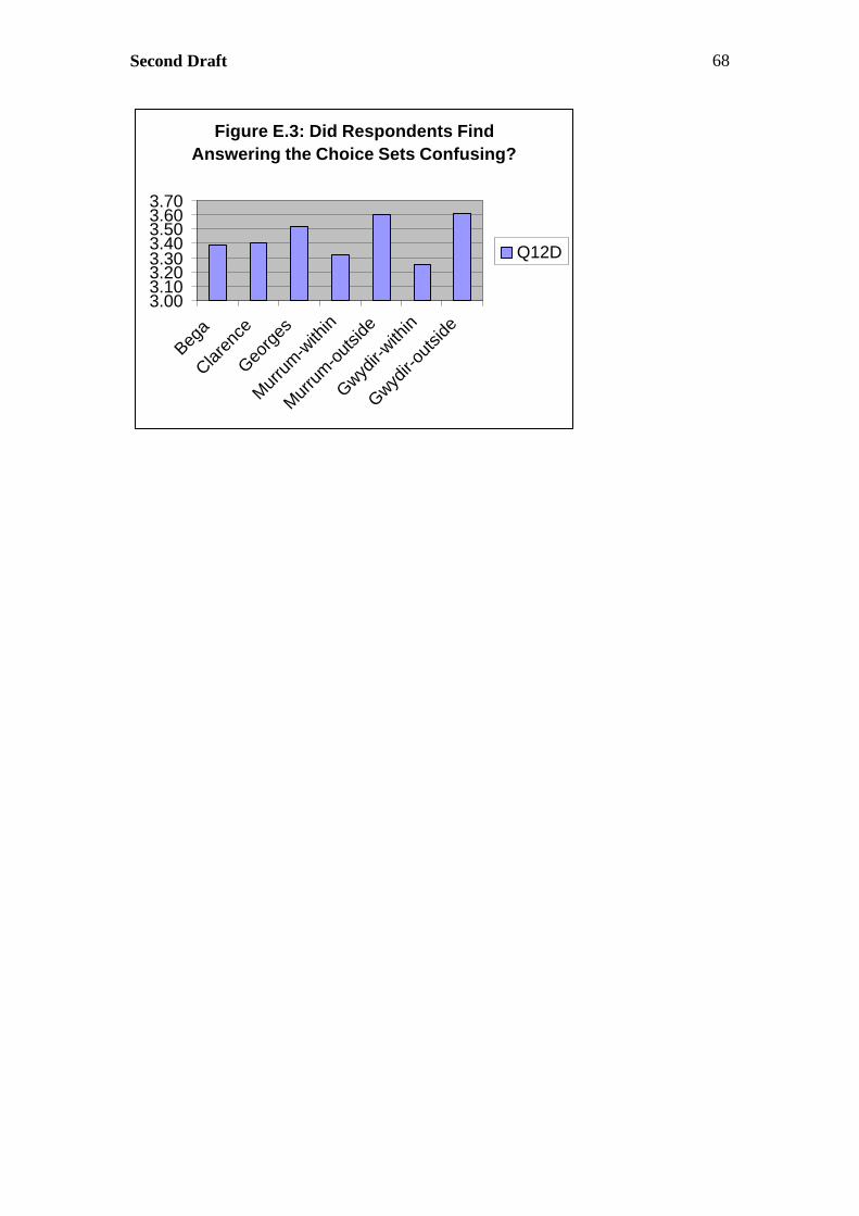
Second Draft 68

Figure E.3: Did Respondents Find Answering the Choice Sets Confusing?

3.003.103.203.303.403.503.603.70

Bega

Claren

ce

Georg

es

Mur

rum

-with

in

Mur

rum

-out

side

Gwydir-

within

Gwydir-

outsi

de

Q12D

Second Draft 69

Appendix F The Benefit Transfer Model

Various researchers have advocated the transfer of demand functions when usingbenefit transfer (eg Desvousges, Naughton and Parsons 1992). The use of choicemodelling provides an example of this sort of transfer, where allowance can be madefor both differences in socio-economic characteristics and within-catchment sitecharacteristics. The development of a benefit transfer model enables an even morerefined use of benefit transfer as allowance is made for differences in catchmentcharacteristics.

The benefit transfer model is presented in Table F.1. The model specification hasbeen deliberately kept simple because of the large number of variables in the model.A multinomial logit model has been used because of problems with the estimation ofthe nested logit model; however, this change in model specification should notsignificantly affect implicit prices (Hausman and Ruud 1987).

Two catchment differences have been included in the model. These are whether thecatchment is inland or coastal (INLAND) and in the north or south of the state(NORTH). The differences have been included through the use of dummy variablesthat have been interacted with the choice set attributes. An additional dummy is alsoused to capture differences in respondent preferences according to whether they residewithin the catchment or outside of the catchment (LOCAL).

This model will allow benefit transfer to a greater variety of catchments than ispossible using transfer only between similar catchments. Value estimates aregenerated for eight different catchment/respondent “scenarios”. This can becontrasted with using benefit transfer between like catchments. In this project fiveindividual catchments have been analysed with two out of catchment samplescollected, a total of seven “scenarios” analysed. Thus this model will enable greateruse of benefit transfer.

The results from this model indicate that:

• Use values are higher in the within catchment samples;• Existence values for vegetation are higher in coastal catchments, and lower if

you are from a within catchment sample;• Existence values for fish species are higher if you are from a coastal

catchment, but lower if you are from a northern coastal catchment;• Existence values for fauna species are not systematically affected by

catchment characteristics;• Respondents to the inland, southern and out of catchment samples were more

likely to choose an option to improve river health;• Respondent’s environmental orientiation (ie progreen or prodevelopment) will

influence their likelihood of choosing an option to improve river health; and• Willingness to pay is a function of sociodemographic characteristics (income

and age).

Second Draft 70

Table F.1: Benefit Transfer Model

Variables Coefficients P-valuesASC1 0.574 0.000ASC2 0.510 0.001ASC * PROGRE 0.379 0.000ASC * PRODEV -0.422 0.000ASC * NORTH -0.240 0.002ASC * LOCAL -0.790 0.000ASC * COASTAL -0.534 0.001RATE -0.009 0.000RATE * INCOME 0.000 0.000RATE * INCOME DUMMY -0.003 0.000RATE * AGE 0.000 0.000VEGETATION 0.022 0.000VEGETATION * LOCAL -0.007 0.000VEGETATION * COASTAL 0.008 0.001FISHABLE 0.171 0.000FISHABLE * LOCAL 0.144 0.009SWIMABLE 0.391 0.000SWIMABLE * LOCAL 0.089 0.112FISH SPECIES 0.037 0.000FISH * COASTAL 0.034 0.015FISH * NORTH * COASTAL -0.048 0.000FAUNA SPECIES 0.010 0.000Summary statisticsLog-likelihood -5786.911Adjusted rho-squared 0.198N 6575

Second Draft 71

Appendix G Attribute Value and Compensating SurplusEstimation Spreadsheet

A spreadsheet decision support tool has been developed to estimate aggregateattribute values and compensating surplus values for specified changes inenvironmental attributes.

The model allows the analyst to specify before and after scenarios of river condition.In addition, the mean levels of income and age in the catchment can be specified toaccount for variations across catchments.

The spreadsheet is shown in Figure G.1. It is found on the accompanying disk on filea:\implicit price_spreadsheet.xls.

Figure G.1: Value estimator spreadsheet

Second Draft 72

Appendix H: State-wide Estimates of the Value ofEnvironmental Attributes of Rivers

At the same time as the individual catchment surveys were being undertaken, aseparate survey of NSW residents’ values for the environmental attributes of riversacross the whole State was carried out. The aim of the additional survey was toidentify the likely extent of framing effects in the outside catchment value estimateswhen multiple rivers are being considered for environmental improvement measures.Because the State-wide sample was drawn from across the whole State, theappropriate comparison to be made is between the outside catchment surveys and theState-wide survey.

The questionnaire used for the State-wide survey was of the same form as used for theindividual catchment surveys apart from two notable features. First, the description ofthe situation respondents were asked to consider was broadened from one river to allthe rivers of the state. Second, the payment vehicle was modified from being a one-offlevy on water rates as used in the individual catchment questionnaire to a levy overthree years. This change in payment vehicle was necessary to reflect the extent of theadditional budgetary pressure the scale of the proposed changes would impose onrespondents. A survey protocol identical to the one used for the individual catchmentswas employed.

The details of the survey response rate and the socio-demographic features of thesample are set out in tables H.1 and H.2 respectively.

Table H.1: Response rate: state-wide survey

State-wide sampleUseable responses 239

Successfully delivered 717Response rate 33.3%

Table H.2: Socio-demographics of sample: state-wide survey

State-widesample

Age (yrs) 52.9Sex (% female)

39%Children 81%

Education# 4.3Income $51,662

# 1-never went to school, 6-tertiary degree

The data collected in the State-wide survey were analysed using a nested logit modelfollowing the same process as was used for the individual catchments’ data (seeAppendix C). The model of respondent choice is displayed in Table H.3.

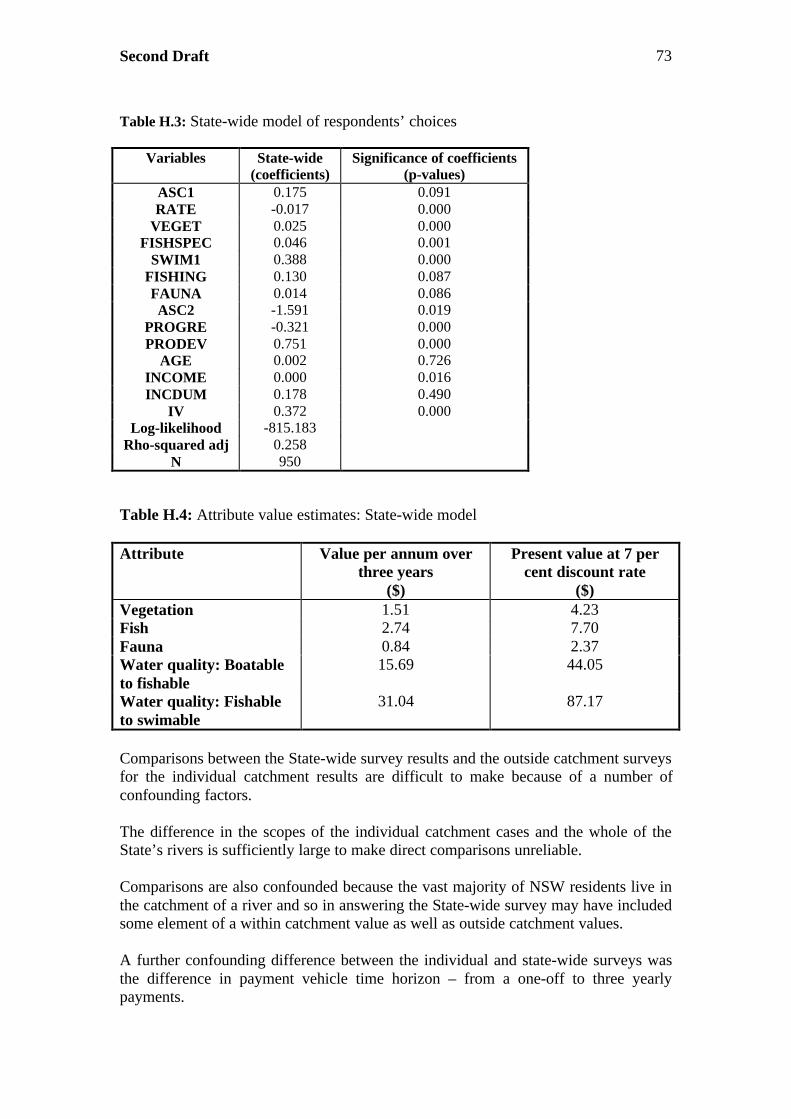
Second Draft 73

Table H.3: State-wide model of respondents’ choices

Variables State-wide(coefficients)

Significance of coefficients(p-values)

ASC1 0.175 0.091RATE -0.017 0.000

VEGET 0.025 0.000FISHSPEC 0.046 0.001

SWIM1 0.388 0.000FISHING 0.130 0.087FAUNA 0.014 0.086ASC2 -1.591 0.019

PROGRE -0.321 0.000PRODEV 0.751 0.000

AGE 0.002 0.726INCOME 0.000 0.016INCDUM 0.178 0.490

IV 0.372 0.000Log-likelihood -815.183

Rho-squared adj 0.258N 950

Table H.4: Attribute value estimates: State-wide model

Attribute Value per annum overthree years

($)

Present value at 7 percent discount rate

($)Vegetation 1.51 4.23Fish 2.74 7.70Fauna 0.84 2.37Water quality: Boatableto fishable

15.69 44.05

Water quality: Fishableto swimable

31.04 87.17

Comparisons between the State-wide survey results and the outside catchment surveysfor the individual catchment results are difficult to make because of a number ofconfounding factors.

The difference in the scopes of the individual catchment cases and the whole of theState’s rivers is sufficiently large to make direct comparisons unreliable.

Comparisons are also confounded because the vast majority of NSW residents live inthe catchment of a river and so in answering the State-wide survey may have includedsome element of a within catchment value as well as outside catchment values.

A further confounding difference between the individual and state-wide surveys wasthe difference in payment vehicle time horizon – from a one-off to three yearlypayments.

Second Draft 74

Given these difficulties, direct comparisons should not be made. The usefulness of theState-wide results is two-fold.

First, they provide an indication of the value held by NSW residents forenvironmental improvements in the state’s rivers. This is important from a policyperspective in terms of the assessment of budgetary priorities for the Stategovernment.

Second, the value estimates provide a boundary for the use of outside catchment valueestimates when framing effects are expected.

Second Draft 75

Appendix I: Status Quo or Business as Usual Levels forEnvironmental Attributes

In each of the choice modelling surveys, respondents were asked to indicate theirpreferred choice of river management options from a selection of three possibilities.In every choice set, one of the three alternatives available was always the status quoor business as usual option. This was defined as the current levels of theenvironmental attributes and a zero levy on water rates. The other alternatives weredefined across the range which attributes could be expected to vary under variousriver management regimes.

The calculation of value estimates for changes in environmental conditions in rivers isbased on a projection of how river attributes will change away from the status quolevels. To facilitate the calculation of these expected changes, the status quo levels forall the environmental attributes of each catchment considered are reported in thisappendix.

Table I.1: Status quo attribute levels

River

Attribute

Bega Clarence Murrum-bidgee

Gwydir Georges

Vegetation (% of riverwith healthy riversidevegetation and wetlands)

30 40 10 10 20

Fish (# of native fishspecies present)

15 22 8 10 12

Fauna (# of waterbirdsand other fauna present)

48 67 60 45 65

Water quality across thewhole of the river (% ofriver)

• Fishable• Swimmable

25%75%

0%21%

38%5%

33%14%

13%67%

valuing the environmental attributes of nsw rivers

Documents