vanet routing on city roads using real-time vehicular ... · nzouonta et al.: vanet routing on city...

IEEE TRANSACTIONS ON VEHICULAR TECHNOLOGY, VOL. 58, NO. 7, SEPTEMBER 2009 3609

VANET Routing on City Roads Using Real-TimeVehicular Traffic Information

Josiane Nzouonta, Neeraj Rajgure, Guiling (Grace) Wang, Member, IEEE, and Cristian Borcea, Member, IEEE

Abstract—This paper presents a class of routing protocolscalled road-based using vehicular traffic (RBVT) routing, whichoutperforms existing routing protocols in city-based vehicularad hoc networks (VANETs). RBVT protocols leverage real-timevehicular traffic information to create road-based paths consistingof successions of road intersections that have, with high probabil-ity, network connectivity among them. Geographical forwardingis used to transfer packets between intersections on the path,reducing the path’s sensitivity to individual node movements. Fordense networks with high contention, we optimize the forwardingusing a distributed receiver-based election of next hops basedon a multicriterion prioritization function that takes nonuniformradio propagation into account. We designed and implemented areactive protocol RBVT-R and a proactive protocol RBVT-P andcompared them with protocols representative of mobile ad hocnetworks and VANETs. Simulation results in urban settings showthat RBVT-R performs best in terms of average delivery rate, withup to a 40% increase compared with some existing protocols. Interms of average delay, RBVT-P performs best, with as much asan 85% decrease compared with the other protocols.

Index Terms—Receiver-based next-hop election, road-basedrouting, vehicular traffic-aware routing.

I. INTRODUCTION

V EHICULAR ad hoc networks (VANETs) are expectedto support a large spectrum of mobile distributed ap-

plications that range from traffic alert dissemination and dy-namic route planning to context-aware advertisement and filesharing [1]–[5]. Considering the large number of nodes thatparticipate in these networks and their high mobility, debatesstill exist about the feasibility of applications that use end-to-end multihop communication. The main concern is whetherthe performance of VANET routing protocols can satisfy thethroughput and delay requirements of such applications. Thispaper focuses on VANET routing in city-based scenarios.

Analyses of traditional routing protocols for mobile ad hocnetworks (MANETs) demonstrated that their performance ispoor in VANETs [6], [7]. The main problem with these pro-

Manuscript received December 14, 2007; revised July 24, 2008 andDecember 23, 2008. First published February 3, 2009; current version pub-lished August 14, 2009. This work was supported in part by the U.S. NationalScience Foundation under Grant CNS-0520033, Grant CNS-0834585, andGrant CNS-0831753. Any opinions, findings, and conclusions or recommenda-tions expressed in this material are those of the authors and do not necessarilyreflect the views of the National Science Foundation. The review of this paperwas coordinated by Dr. L. Cai.

The authors are with the Department of Computer Science, New JerseyInstitute of Technology, Newark, NJ 07102 USA (e-mail: [email protected];[email protected]; [email protected]; [email protected]).

Color versions of one or more of the figures in this paper are available onlineat http://ieeexplore.ieee.org.

Digital Object Identifier 10.1109/TVT.2009.2014455

tocols, e.g., ad hoc on-demand distance vector (AODV) [8] anddynamic source routing (DSR) [9], in VANET environmentsis their route instability. The traditional node-centric view ofthe routes (i.e., an established route is a fixed succession ofnodes between the source and the destination) leads to frequentbroken routes in the presence of VANETs’ high mobility, as il-lustrated in Fig. 1(a). Consequently, many packets are dropped,and the overhead due to route repairs or failure notificationssignificantly increases, leading to low delivery ratios and hightransmission delays.

One alternative approach is offered by geographical routingprotocols, e.g., greedy–face–greedy (GFG) [10], greedy otheradaptive face routing (GOAFR) [11], greedy perimeter statelessrouting (GPSR) [12], which decouple forwarding from thenodes identity. These protocols do not establish routes but usethe position of the destination and the position of the neighbornodes to forward data. Unlike node-centric routing, geograph-ical routing has the advantage that any node that ensuresprogress toward the destination can be used for forwarding.For instance, in Fig. 1(a), geographical forwarding could usenode N2 instead of N1 to forward data to D. Despite better pathstability, geographical forwarding does not also perform wellin city-based VANETs [6], [13]. Its problem is that, oftentimes,it cannot find a next hop (i.e., a node that is closer to thedestination than the current node). For example, as shown inFig. 1(b), it can take road paths that do not lead to the desti-nation. The recovery strategies in the literature are often basedon planar graph traversals, which were shown to be ineffectivein VANETs due to radio obstacles, high node mobility, and thefact that vehicle positions are constrained on roads rather thanbeing uniformly distributed across a region [6].

A number of road-based routing protocols [6], [7], [13], [14]have been designed to address this issue. However, several pro-tocols [6], [14] fail to factor in the vehicular traffic flow by usingthe shortest road path between the source and the destination.As depicted in Fig. 2, it is possible that the road segments on theshortest path are empty (or have network partitions). Otherprojects [13], [15]–[17] try to alleviate this issue by using his-torical data about average daily/hourly vehicular traffic flows.Unfortunately, historical data are not accurate indicators of thecurrent road traffic conditions, because events such as roadconstructions or accidents that lead to traffic redirection arenot rare.

This paper presents a class of road-based VANET routingprotocols that leverage real-time vehicular traffic informationto create paths consisting of successions of road intersectionsthat have, with high probability, network connectivity amongthem. Furthermore, geographical forwarding allows the use

0018-9545/$26.00 © 2009 IEEE

3610 IEEE TRANSACTIONS ON VEHICULAR TECHNOLOGY, VOL. 58, NO. 7, SEPTEMBER 2009

Fig. 1. Problems with traditional routing approaches in VANETs. (a) Routes that were established as fixed successions of nodes frequently break in highlymobile VANETs. Route (S, N1, D) that was established at time t breaks at time t + Δt when N1 moves out of the transmission range of S. (b) Geographicalrouting can route packets toward dead ends, causing unnecessary traffic overhead in the network and longer delays for packets. Instead of forwarding data on thedotted path, geographical routing sends data to N1 and N2, following the shortest geographical path from S to D on a dead-end road.

Fig. 2. Our solution creates a route (S, I1, I2, I3, D) using the road intersec-tions. Since it considers the real-time vehicular traffic, our solution can avoidthe shorter path (S, I1, I3, D) that would lead to a broken route. Once theroad-based route is established, geographical forwarding is used to route databetween any two intersections.

of any node on a road segment to transfer packets betweentwo consecutive intersections on the path, reducing the path’ssensitivity to individual node movements. Fig. 2 shows oneexample that illustrates the main idea of this class of routing,which we call road-based using vehicular traffic (RBVT) rout-ing. The RBVT class of routing presents two main advantages:1) adaptability to network conditions by incorporating real-time vehicular traffic information and 2) route stability throughroad-based routes and geographical forwarding. We present twoRBVT protocols: 1) a reactive protocol RBVT-R and 2) a proac-tive protocol RBVT-P. RBVT-R discovers routes on demandand reports them back to the source, which includes them inthe packet headers (i.e., source routing). RBVT-P generatesperiodical connectivity packets (CPs) that visit connected roadsegments and store the graph that they form. This graph is thendisseminated to all nodes in the network and is used to computethe shortest paths to destinations.

Our initial NS-2 simulations with an IEEE 802.11 VANETshowed that, when the wireless medium becomes congested,the overhead introduced by the periodic “hello” packets formaintaining the list of neighbors in geographical forwardingsignificantly degraded the end-to-end data transfer performance.

To reduce this overhead, we propose a beaconless distributedreceiver-based election of next hop, considering nonuniformradio propagation. This method uses a light modification ofthe request-to-send/clear-to-send (RTS/CTS) mechanism in theIEEE 802.11 standard. A multicriterion prioritization functionis introduced to select the best next hop by using the distancebetween the next hop and the destination, the received powerlevel (which could be affected by noise and channel fading),and the distance to the transmitter as parameters.

We evaluate the performance of the proposed protocols usingtwo scenarios: 1) an urban environment with obstacles usingperiodic “hello” messages and the standard 802.11 mediumaccess control (MAC) protocol (node movements are generatedusing the open-source microscopic traffic generator simulationof urban mobility (SUMO) [18], which has been validatedagainst real vehicular traces) and 2) an urban environmentwithout obstacles, using the proposed forwarding optimizationfor the RBVT protocols. This scenario tests the protocols inhigh-contention environments. In these tests, we used a ve-hicular traffic generator that we developed based on the car-following model proposed by Gipps [19], [20]. This modelenables vehicles to move at the maximum safest speed whileavoiding collisions.

The simulation results show that the RBVT protocols out-perform existing protocols in both studied scenarios. In termsof successful data delivery, RBVT-R performed best, with anincrease of as much as 40% compared with AODV and 30%compared with GSR using the IEEE 802.11 standard. In termsof the average delay, RBVT- P performed best, with delays of asmuch as 85% lower than existing solutions. The proposed for-warding optimization provided noticeable improvements in thehigh-contention scenario. The scenario with obstacles yieldedbetter performance, even without using the optimization. Thiscase was the result of lower contention in the network and thefact that RBVT protocols forward data along the roads and notacross the roads.

The rest of this paper is organized as follows. Section IIpresents the two RBVT protocols. Section III describes theoptimized forwarding mechanism. Section IV presents thesimulation results. The related work is reviewed in Section V,and this paper is concluded in Section VI.

NZOUONTA et al.: VANET ROUTING ON CITY ROADS USING REAL-TIME VEHICULAR TRAFFIC INFORMATION 3611

Fig. 3. Route establishment in RBVT-R. (a) A source node uses our improved flooding mechanism to send a route discovery packet in the network to find thedestination. The route discovery packet is broadcast along the roads and stores the traversed intersections in its header. (b) The destination unicasts a route replypacket back to the source. The reply follows the route that was stored in the route discovery packet, and geographical forwarding is used between intersections.

II. RBVT PROTOCOLS

The RBVT routing protocols leverage real-time vehiculartraffic information to create road-based paths. RBVT paths canbe created on demand or proactively. We designed and imple-mented two RBVT protocols, each illustrating a method of pathcreation: 1) a reactive protocol RBVT-R and 2) a proactiveprotocol RBVT-P. The RBVT protocols assume that each ve-hicle is equipped with a GPS receiver, digital maps (e.g., TigerLine database [21]), and a navigation system that maps GPS po-sitions on roads. Vehicles exchange packets using short-rangewireless interfaces such as IEEE 802.11 [22] and dedicatedshort-range communication (DSRC) [23].

A. RBVT-R: Reactive Routing Protocol

RBVT-R is a reactive source routing protocol for VANETsthat creates road-based paths (routes) on demand by using“connected” road segments. A connected road segment is asegment between two adjacent intersections with enough ve-hicular traffic to ensure network connectivity. These routes,which are represented as sequences of intersections, are storedin the data packet headers and are used by intermediate nodesto geographically forward packets between intersections.

1) Route Discovery (RD): When a source node needs tosend information to a destination node, RBVT-R initiates aroute discovery process, as illustrated in Fig. 3(a). The sourcecreates an RD packet, whose header includes the address andlocation of the source, the address of the destination, and asequence number. We assume unique addresses for nodes. RDis flooded in the region around the source to discover a routetoward the destination. The flooding is necessary, becauseRBVT-R does not assume a location service that can be queriedto find out the location of the destination. For scalabilityreasons, the flooding region is limited by a time-to-live (TTL)value that is set in the header.

To reduce the effects of the broadcast storm problem [24],RBVT-R uses an improved flooding mechanism similar to [25].If a node receives an RD packet with the same source address

and sequence number with a previously received packet, itdiscards the RD packet. When a node receives a new RD, itdoes not directly rebroadcast this packet; the node holds thepacket for a period of time inversely proportional to the distancebetween itself and the sending node. Once the waiting periodis over, a node rebroadcasts the RD packet only if it did notnotice that this packet was rebroadcast by nodes that are locatedfarther on the same road segment. This way, farther nodes canfirst rebroadcast the request, thus ensuring faster progress andless traffic in the network.

In RBVT-R, the route is gradually built. Initially, the routestored in the RD packet is an empty list. When a node receivesthe RD packet for the first time, it checks if it is located ona different road segment from the transmitter of the packet.If so, the receiving node appends to the route list the roadintersections that were “traversed” by the RD packet from thetransmitter position. We illustrate the route creation processusing Fig. 3(a). The source vehicle S creates an RD packetto discover a route to destination D. S adds its own positionin the packet and broadcasts it. Both nodes A and B receivethe packet on segment I1–I6, but only B will rebroadcast it inthe improved flooding mechanism. Before this rebroadcast, Bappends intersection I1 to the route in the header of the packet.However, when C receives the RD packet, it will not update theroute, because C is on the same road segment with B. A newintersection I6 is added at node E. This process continues untilthe packet reaches the destination or the TTL expires.

The RD packet may sometimes be received by nodes onparallel streets. In this case, the RD packet is updated only ifthe sequence of intersections that were implicitly traversed canbe determined. If this condition is not possible, we prevent, inour implementation, those nodes from updating the RD packets.The route structure is stored in the header of the RD packet;thus, the number of intersections that can be appended to aroute is limited by the size of the IP packet header optionsand the number of bytes for identifying each road intersection.Techniques such as hierarchical naming of intersections (i.e.,identifying the city and then the intersections within the city)


can increase the maximum number of intersections that arestored in RD.

2) Route Reply (RR): Upon receiving the RD packet, thedestination node creates an RR packet for the source. The routethat is recorded in the RD header is copied in the RR header. Asshown in Fig. 3(b), this route defines a connected path, whichis composed of road intersections, from the source to the desti-nation. The destination also adds its current position in the RRheader. The RR packet is forwarded along the road segmentsthat are defined by the intersections in its header. Geographicalforwarding is used between intersections to take advantage ofevery available node on the path. The destination may receiveduplicates of an RD packet. A new reply is generated only ifthe newly received packet contains a route of better quality.The quality of a route can be expressed using a combination ofmetrics such as node density on the road segments, the numberof lanes, and traffic-flow rates. In the current implementation,the fewer the number of intersections, the better the route. Uponreceiving the RR packet, the source starts sending data. Eachdata packet stores the route in its header, and it is geographicallyforwarded along this route. Protocol 1 presents the pseudocodefor the RD and RR phases.

Protocol 1: RD and RR in RBVT-R at node ni

Notation:nS and nD: ID of the source and the destinationPath and TempPath: Best and temporary paths fromnS to nD

|Path|: Path lengthRS(ni): Road segment where node ni is locatedα: Waiting-time parameterRD: RD packetRR: RR packet

Upon receiving RD(nS , nD, T empPath) from nj

1: if (ni == nD)&(|TempPath| ≤ |Path|) then2: Path = TempPath3: Send RR(nD, nS , Path)4: Return5: end if6: if RD not seen before then7: if (RS(ni) �=RS(nj))&(RS(ni) /∈TempPath) then8: Add RS(ni) to TempPath9: end if10: Set timer = α ∗ distance(nj , ni)11: else12: if RS(ni) == RS(nj) then13: Cancel timer /∗nj is a better broadcast node ∗/14: end if15: end if

Upon timeout16: Broadcast RD(nS , nD, T empPath)

Upon receiving RR(nD, nS , Path) from nj :17: if ni == nS then18: Store Path19: Forward Data(Path)

20: else21: Forward RR(nD, nS , Path)22: end if

3) Route Maintenance: Existing routes are updated to adaptto the movements of the source and the destination over timeand to repair broken paths. Sources and destinations are movingvehicles; thus, the route that was created during the RD phaseis not expected to remain constant. We use a dynamic routeupdating technique at the source to keep the route consistentwith the current road segment positions of the source and thedestination nodes. For instance, if node S in Fig. 3(b) movesto segment I1–I6, I1 is no longer a valid intersection along theroute and should be removed. This change takes place at thesource, which also informs the destination of the new path usingroute update (RU) control packets. Similarly, node D may moveto road segment I5–I8. When this happens, I8 should be re-moved from the list of intersections in the route. Consequently,the destination sends an RU packet to the source. If this updateis received at the source, it means that the route is valid, and itcan, therefore, be used for future data transmissions.

In some situations, the vehicle node may transmit the RUpacket before changing the road segment. For example, if avehicle node is about to make a turn that will result in theaddition of an intersection to the path, the presence of obstaclesmay temporarily cause a loss in connectivity [26], which mayprevent the successful transmission of the update packet. Toavert this problem, vehicle nodes with RBVT-R can transmitthe RU packet before the turn to the new segment is complete.

A route error occurs when no forwarding node can be foundto reach the next intersection in the route. In this case, the nodethat detected the problem unicasts a route error packet to thesource. We observed that, sometimes, broken routes are onlytemporary. Therefore, to reduce the flooding associated withthe RD process, the source does not generate a new RD packetas soon as it receives a route error notification. Upon such anotification, it puts the respective route on hold for a certaintimeout. Packets toward that destination are queued until theexpiration of the hold timeout. The source then attempts to usethe same route. An RD is generated only after a few consecutiveroute errors.

B. RBVT-P: Proactive Road-Based Routing

RBVT-P is a proactive routing algorithm that periodicallydiscovers and disseminates the road-based network topology tomaintain a relatively consistent view of the network connec-tivity at each node. Each node uses this (near) real-time graphof the connected road segments to compute shortest paths toeach intersection. RBVT-P assumes that a source can query alocation service (e.g., GLS [27]) to determine the position ofthe destination when it needs to send data.

1) Topology Discovery: Proactive routing algorithms [28]use various forms of flooding to discover and update the net-work topology. To keep up with VANET’s mobility, floodingmay be required quite often, and the routing overhead wouldlead to heavy congestion in the network. In RBVT-P, how-ever, we can limit flooding frequency, because we are mainly


Fig. 4. Route establishment in RBVT-P. (a) Generator nodes periodically unicast CPs to discover the road-based network topology. The path of one CP is depictedstep by step as it visits and records all road segments with enough vehicular traffic to maintain connectivity between endpoints. As shown between intersectionI4 and I1, the CP creates a virtual intersection when a road segment has partial traffic, but a network partition precludes it from reaching the next intersection.(b) The CP returns to the segment of its generator with the network topology graph shown in this figure, which contains all the road segments with traffic on them.Note that segments with partial traffic are considered by adding virtual intersections. Then, a route-update packet that contains this graph is disseminated to allnodes in the network. Upon receiving a route update, each node updates its routing table and recomputes the shortest paths to all intersections.

interested in discovering the road-based network topology.More precisely, the goal of RBVT-P is to capture the real-time view of the traffic on the roads. Thus, the fact that theconnectivity between certain nodes on a road segment changesover time does not matter as much, as long as that road segmentremains connected. This situation is highly probable on roadswith relatively dense vehicular traffic.

The road-based network topology is constructed using con-nectivity packets (CPs) that were unicast in the network. CPstraverse road segments and store their endpoints (i.e., inter-sections) in the packet. CPs are periodically generated by anumber of randomly selected nodes in the network. Each nodeindependently decides whether it will generate a new CP basedon the estimated current number of vehicles in the networks, thehistoric hourly traffic information, and the time interval since ithas last received a CP update. When creating a new CP, a nodedefines the road-based perimeter of the region to be covered bythe CP and stores it in the CP. This step is necessary both tolimit the time spent by the CP in the network, which implicitlydefines the freshness of its information, and to ensure that thisinformation fits in one packet. CPs traverse the road map usingan algorithm that was derived from a depth-first search (DFS)graph traversal but, unlike DFS, the road intersections (vertices)are not added to the stack at the beginning of the traversal.Rather, vertices are progressively added to the CP stack asthe CP reaches adjacent road segments. We use flags (i.e., Ufor unreachable, R for reachable, and I for initialized) to keeptrack of the state of the intersections in the CP stack. Networkpartitions may preclude the CP from visiting the entire graph.We discuss this issue in Section II-B4. Fig. 4(a) illustrates howone CP sequentially visits connected road segments and returnswith the topology information to its generator segment. The CPtraversal ends at the road segment of the initiator. Any vehiclethat first receives the CP on that segment after all markedintersections have been visited will disseminate the CP content.

2) Topology Dissemination: The network topology infor-mation in the CP is extracted and stored in an RU packetthat is disseminated to all nodes in the network (i.e., in theregion covered by the CP). Fig. 4(b) shows the CP/RU contentassociated with the topology in Fig. 4(a). The RU is markedwith a timestamp to indicate the freshness of its information(i.e., because nodes have GPS receivers, they can use the GPStime, which varies insignificantly among different receivers).Upon receiving an RU packet, nodes update their local routingtable to reflect the newly received information.

Each node maintains a routing table with entries of the form

〈Intersectioni, Intersectionj , State,

T imestamp,Entry_timeout〉

where state is equal to R or U . R means that the intersectionis reachable, whereas U means that it is unreachable. Thetimestamp is taken from the RU packet during the update.The entry_timeout is a function of the CP generation periodand allows the node to purge old information when no newupdates about certain intersections are received. When a nodereceives an RU, it does not replace its entire routing tablewith the new topology, but rather, it updates its routing tableon a segment-by-segment basis. This type of update allowseach node to aggregate information from multiple RUs intoits local routing table. Note that it is possible to receive in-formation from multiple RUs that visited overlapping regions.Protocol 2 presents the pseudocode for topology discovery anddissemination.

Protocol 2: Topology discovery and dissemination inRBVT-P at node ni

Notation:nO: ID of the node that originated the CPIl: Intersection l


Ini: Intersection that is closest to ni

〈Il, Im〉: Road segment between consecutive intersec-tions Il and Im

Stack: Stack of road segments that will be visitedS: Set of all road segmentsRS(ni): Road segment where node ni is locatedα: Waiting-time parameterCP: CPRU: RU packet

Upon receiving CP(nO):1: if proximity(ni, Il) then2: for each 〈Il, Ik〉 do3: if 〈Il, Ik〉 /∈ Stack then4: Add 〈Il, Ik〉 to Stack5: end if6: end for7: if Ini

== InO&Stack == φ then

8: Broadcast RU(ni)9: Return10: end if11: if RS(ni) == 〈Il, Im〉 & (all 〈Im, Ik〉 in Stack‖

marked in S) then12: Mark the reachability of 〈Il, Im〉 in S/∗ R—

reachable; U—unreachable ∗/13: Remove 〈Il, Im〉 from Stack14: end if15: Read 〈Il, Im〉 from the top of Stack16: Forward CP(nO) toward Im/∗ Send to the next hop

toward Im ∗ /17: end if

Upon receiving RU(nO) from nj :18: if RU(nO) not seen before then19: Update the local routing table with RU(nO) data20: Set timer = α ∗ distance(nj , ni)21: else22: if RS(ni) == RS(nj) then23: Cancel timer24: end if25: end if

Upon timeout26: Broadcast RU(nO)

3) Route Computation: A source node computes the short-est path to the destination by using only road segments thatare marked as reachable in its routing table. The sequence ofintersections that denote the path is added to the header ofeach data packet. This header includes the timestamp that isassociated with the route to allow for freshness comparisons atintermediate nodes.

Once the route is computed, RBVT-P uses loose sourcerouting to forward data packets to improve the forwardingperformance. The idea is to quickly forward the packet whenthe intermediate nodes have the same or older information thanthe source and, at the same time, take advantage of fresherinformation when available.

4) Route Maintenance: Intermediate nodes with fresher in-formation update the path in the header of data packets. In caseof a route break, the intermediate node switches to geographicalrouting, which is used until the packet reaches a node that hasfresher information, and consequently, a new route is stored inthe packet header.

One important consideration is the number of CPs that areneeded in the network. RBVT-P generates multiple CPs fromdifferent positions in each update period. This condition isneeded to ensure redundancy in the event of CP losses ornetwork partitions, which could frequently happen in highlyvolatile VANETs. Indeed, in case of a network partition, thenodes in the partition from which the CP was generated wouldstill receive updated information on that part of the network,as well as knowledge of disconnections. However, nodes inany other partition would no longer receive updates until thepartition is bridged. Thus, there is a need to instantiate CPsfrom different positions in the network. The presence of mul-tiple CPs, however, raises consistency issues, because a nodemay receive RU updates from multiple sources. This problemis solved using the RU timestamps, as we have previouslydescribed.

III. FORWARDING OPTIMIZATION

Our initial simulation results with RBVT protocols showedthat, as the network became congested, the overhead trafficfrom periodic “hello” messages negatively created an impact onthe end-to-end data transfers. This section presents our solutionto this problem, i.e., a distributed next-hop election method,which significantly increases the average data delivery ratio byreducing the overhead associated with the selection of the next-hop node in congested networks.

In RBVT, geographical forwarding is used to transfer datapackets between intersections. In previous works on geograph-ical or position-based forwarding [10]–[12], each forwardingnode picks the next hop by using its list of neighbors and theirgeographical positions. The next hop is chosen in such a waythat the forwarding progress is maximized (e.g., typically, this isthe neighbor closest to the destination). This process continuesuntil the packet reaches the destination. Therefore, to success-fully choose next hops, it is vital for each en-route node to keepa precise neighbor list. If the lists are not accurate, the best nexthop could be missed, or even worse, a node that is alreadyout of the transmission range could be chosen. Maintainingup-to-date lists requires frequent “hello” packet broadcasting.However, this broadcasting results in a large communicationoverhead.

We propose a solution that was inspired by the receiver-basedrelay election approaches (e.g., [29]–[31]) in ad hoc and sensornetworks to eliminate “hello” packets. In these approaches, thesender broadcasts a control packet that informs its neighborsabout a pending data packet transmission. Each receiver usescertain criteria to determine if it should elect itself as a next-hopcandidate, and if so, it computes a waiting time. This waitingtime is used to allow better receivers to answer first. If a receiverdoes not overhear a better candidate before its waiting timeexpires, it informs the sender that it is the best next hop.


Fig. 5. RTS/CTS exchange in the IEEE 802.11 with DCF standard.

The current implementations of these approaches use onecriterion for computing the waiting time, i.e., the distancebetween potential next hops and the destination. This methodworks well under the unit-disk assumption (i.e., the transmis-sion range is a circle of a fixed radius). However, previousstudies (e.g., [32]) have shown that real wireless radios do notfollow the unit-disk assumption. This is particularly true invehicular networks where buildings and other obstacles createan impact on radio propagation through signal fluctuations andfading. In this context, selecting the neighbor that optimizes theforward progress alone does not guarantee an optimal selectionof the next hop [33].

The method proposed here accounts for nonuniform radiopropagation that uses two additional criteria: 1) optimal trans-mission area and 2) received power. Furthermore, our next-hop election protocol piggybacks its data on the IEEE 802.11RTS/CTS frames [22], thus introducing no overhead. To helpwith the understanding of this protocol, we continue the presen-tation with a brief overview of the IEEE RTS/CTS mechanism.

A. 802.11 RTS/CTS Background

In the IEEE 802.11 with distributed coordination function(DCF) standard, the RTS and CTS frames are used to addressthe hidden terminal problem that is inherent to wireless com-munications. This problem and the functionality of RTS/CTSframes are illustrated in Fig. 5. In this example, both node Sand node C are node B’s neighbors. When S sends a frame toB, C should not send any frame to B; otherwise, there would bea collision at B. However, node C is out of the communicationrange of node S, and it does not detect a busy channel while Sis transmitting. Once node C starts its transmission, a collisionhappens at B, which cannot be detected by S until after it timesout without receiving an acknowledgment from B.

IEEE 802.11 with DCF addresses the hidden terminal prob-lem by deploying the RTS/CTS exchange. Before a node trans-mits a frame, it sends a very short RTS frame to the intendedreceiver, including the transmission time of the follow-up dataand acknowledgment frames. The receiver broadcasts a CTSmessage, which is received by all its neighbors, once it receivesthe RTS with the needed channel clear time. The neighbors willconsequently defer their transmissions until this transmission iscompleted. In the example, node C will never send to node Bwhile node S is sending to node B, because node C has heardthe CTS from node B. Node C will wait for the time specified

in the CTS to guarantee that the transmission from S to B issuccessful.

B. Election Using RTS/CTS

RBVT leverages the RTS/CTS exchange to replace thesender selection of the next hop with a receiver self electionand implicitly eliminates the overhead associated with frequent“hello” messages in geographical forwarding in congested net-works. In essence, broadcasts of RTS frames become requestsfor next-hop self election. RTS frames are modified to carry theposition of the sender and the position of the target destination,which are used during the self election. RTS frames also carrya flag to indicate to all receiving nodes that they should processand, possibly, answer the frame (in the original mechanism,only the intended receiver processes and answers an RTSframe).

In particular, each node that receives the modified RTS framecalculates a waiting time, after which it will send a CTS frameback to the sender. The waiting time is an indicator of how goodthe node is a forwarding candidate; i.e., the shorter the waitingtime is, the better candidate the node becomes. Section III-Cexplains how this waiting time is calculated. A CTS from oneof the receivers indicates that a better candidate exists, andno candidate receivers that overhear it will reply. The senderreceives the CTS from the best next-hop candidate and forwardsthe data frame to this node, which then acknowledges the dataframe. The detailed protocol is presented in Protocol 3.

Protocol 3: Self-election algorithm at node ni

Notation:tDATA, tCTS, tRTS, and tACK: time to transmit the dataframe, CTS, RTS, and ACKti: waiting time of node ni

loci: location of node ni

locD: location of the destinationnS : ID of the sender that looks for the next hop

Upon receiving RTS(locs, locD, tDATA) from node ns:1: Call the waiting function and calculate ti2: Set the timer to ti3: Defer transmissions, if any, for tDATA + tRTS

Upon receiving an CTS(nj , ns, tDATA) from nj before thetimeout4: Cancel the timer / ∗ nj is the best next-hop candidate ∗/5: Defer transmissions, if any, for tDATA

Upon overhearing DATA from node ns

6: Defer transmissions, if any, for tACK

Upon timeout:7: Broadcast CTS(ni, nS , tDATA)/ ∗ ni is the best candidate∗/

Fig. 6 shows an example that illustrates this protocol. SendernS needs to forward a data frame to the best next hop thatis en route to destination D. It broadcasts an RTS frame byspecifying its own location, the location of destination D, and


Fig. 6. Next-hop self-election example. (a) RTS broadcast and waiting-timecomputation. (b) CTS broadcast. (c) Data frame. (d) ACK unicast.

the transmission time of the data frame. Nodes n1, n2, and n3

hear the RTS, calculate their waiting time, and set their timersto wait before replying to nS with CTS. Note that n4 doesnot perform the computation, because it is farther from thedestination compared to the sender. Node n2 has the shortestwaiting time and replies with the CTS first. Once n1 and n3

overhear the CTS from n2, they will cancel their timers. Inaddition, all the neighbors of n2, will know that they should notsend any frame to n2 until it completes the transmission. OncenS receives the CTS from n2 it will send the data frame to n2.At the same time, all of nS’s neighbors that overhear the dataframe learn that they should not send any frame to nS untiln2 finishes sending the acknowledgment to nS . This exampleshows how this forwarding method can effectively choose thenext hop without any “hello” message overhead.

C. Waiting Function

Determining the best next hop depends on the waiting time.An effective calculation of this waiting time should meet threeobjectives: 1) The waiting time of the best next-hop candidate isthe shortest time such that this node replies first; 2) the waitingtime difference between the best next-hop candidate and thesecond best candidate is large enough such that collisions areminimized between nearby nodes; and 3) the waiting time isas short as possible to avoid unnecessary delays. To achievethese goals, we first identify three key parameters—forward

Fig. 7. Sample translation functions for the optimal transmission area.

progress, optimal transmission area, and received power—thatcharacterize the best next hop and then incorporate them withdifferent weights into a low-complexity function that computesthe waiting time.

1) Function parameters: The forward progress di of a nodeNi from a sender S is defined as di = dSD − dNiD, where dSD

is the distance between the sender S and the destination D, anddNiD is the distance between Ni and D. This parameter is com-monly used in the geographical forwarding of single-criterionreceiver-oriented schemes [29], [30], [34]. It denotes the actualprogression that the packet made toward the destination if Ni

would be the next hop. A node with di that is closest to dSD isthe node closest to the destination.

The optimal transmission area fi of a node Ni describes theprobability that the node can successfully receive the sender’sdata packet. Wireless channels are error prone; thus, a node thatis located much farther than the nominal transmission rangemay not successfully receive long data frames, although it canreceive short RTS frames without errors. This situation couldhappen because real wireless radios do not follow the unit-diskassumption [32].

We deploy a translation function to express the optimaltransmission area. The function takes the distance to the senderas input and outputs the distance to the optimal transmissionarea. Sample graphs for two translation functions are depictedin Fig. 7, and one of these functions is defined as follows:

ftrans(x) ={

x + dtrans, if x ≤ dopt

−x + dmax, if x > dopt

where dopt represents the optimal transmission range, dmax

represents the estimated maximum transmission range for anacceptable error rate, and dtrans represents the translation dis-tance (dtrans = 150 m for ftrans in Fig. 7). These parametersmay be adjusted based on the network conditions in the area.

The received power pi of a node Ni is the received powerlevel of the RTS frame. Priority is given to nodes with strongerpi. This parameter indicates the true channel quality from asender to a receiver. Empirical studies and theoretic analysis canprovide an optimal transmission area, but in reality, there can beobstacles or noise around nodes. The received power can also


help in differentiating nodes at comparable distances. The factthat the reporting of the received signal power is made while thevehicles are moving does not affect the quality of the reporteddata, because the distance a vehicle travels while receiving anRTS is negligible.

2) Function definition: We adapt the multivariable functionin [33] and customize it to a three-variable polynomial of theselected parameters. The waiting time ti returned by this func-tion is in the interval [0, Tmax], where Tmax is the maximumwaiting time. We have

f(di, dSNi, pi) = Adα1

i fα2i pα3

i + Tmax

where A = (−Tmax/(dα1maxf

α2maxp

α3max)), and αi(i = 1, 2, 3) is

the weight of each parameter.The greater the weight value is, the greater the impact that the

parameter has in the election process. All next-hop candidatesuse the same values of parameters αi. We currently use staticvalues for these factors, but they could dynamically be deter-mined and adjusted based on the network and traffic conditionsin the area.

3) Function evaluation: Fig. 8 shows a comparison betweenthe next-hop selection that uses the multicriterion function andthe selection that uses only the forward-progress parameter. Weconsider a transmitter at location (0, 0) and a destination atlocation (800, 200). The waiting time for the nodes after theyreceive an RTS frame if they were located at various locationsaround the transmitter is shown in Fig. 8(a) and (b). In thiscomparison, we used the following coefficients in the multi-criterion function: 1) α1 = 0.2, 2) α2 = 1.2, and 3) α3 = 0.03.The optimal wireless transmission range is set to be 250 m, andthe translation function ftrans in Fig. 7 is deployed. Note thatperfect reception within a specific range around the transmitteris not assumed. Rather, the received power is calculated usingthe shadowing propagation model [35]. In this model, the powerlevel at a receiving node is not solely a function of the distanceto the transmitting node, but randomness is added to account forfluctuations in signal propagation. The formula for computingthe received power is

∣∣∣∣ Pr(d)Pr(d0)

∣∣∣∣dB

= −10β log(

d

d0

)+ XdB (1)

where XdB is a normal random variable with mean zero andstandard deviation σdB. σdB is the shadowing deviation, and βrepresents the path-loss exponent.

The comparison in Fig. 8 shows that the proposed schemefavors nodes around the optimal transmission range and as-signs shorter waiting times for the nodes within this range.The forward-progress-only approach favors nodes beyond theoptimal transmission range (in case they receive the RTS),which could lead to many data packet losses. Table I validatesthis observation, because it presents a comparison betweenthe two methods in terms of packet loss and the number ofMAC-layer frames that were transmitted in the network per datapacket that was successfully received at destinations (which isa measure of traffic overhead). These simulation results were

Fig. 8. Waiting times that were experienced by receivers located at various po-sitions around a transmitter. (a) Waiting time that was determined using forwardprogress only. (b) Waiting time that was determined using the multicriterionfunction.

TABLE IUSING THE MULTICRITERION FUNCTION TO SELECT NEXT HOPS

LEADS TO SIGNIFICANTLY LOWER PACKET LOSS AND OVERHEAD

COMPARED WITH USING FORWARD PROGRESS ONLY

obtained using RBVT-R in a network with 250 nodes. Fifteensource–destination pairs exchanged 10 000 packets at the rateof 2 packets/s. Using the multicriterion function leads to apacket loss that is five times lower than using forward progressonly. In addition, the traffic overhead is more than one orderof magnitude lower when using the proposed scheme. Thisresult is due, in part, to the large number of retransmissionsthat were experienced by nodes located farther from the optimaltransmission range.


IV. PERFORMANCE EVALUATION

This section presents the evaluation of the RBVT protocolsusing the network simulator NS-2.30 [36]. To evaluate theperformance, we use two urban scenarios: 1) a scenario withobstacles to model buildings, in which we make use of periodic“hello” messages and the IEEE 802.11 with DCF standard,and 2) a scenario without obstacles to simulate high-contentionnetworks, for which optimized forwarding is used. We compareRBVT-R and RBVT-P with four existing VANET/MANETrouting protocols. In the following, we present the evaluationmethodology, the metrics for comparing the protocols, and theanalysis of the simulation results.

A. Evaluation Methodology

We compare the performance of the RBVT protocols withrepresentatives from the main classes of routing protocols:

1) AODV [8], which is a MANET reactive routing protocol;2) OLSR [28], which is a MANET proactive routing

protocol;3) GPSR [12], which is a MANET geographical routing

protocol;4) GSR [6], which is a VANET position-based routing

protocol that takes into account the road layouts in theforwarding decisions.

We now briefly review how each of these protocols operate.In AODV, a route is created on demand when a source node

wants to communicate with a destination node. The route cre-ation involves flooding a route request message and establish-ing, at each hop, a backward pointer (the last transmitter of therequest) to the source. A reply is unicast along this path by usingthe backward pointers while establishing forward pointers tothe destination. In OLSR, each node maintains sets of one- andtwo-hop neighbors and selects some neighbors as multipointrelays. OLSR proactively discovers and disseminates link-stateinformation over the multipoint relays backbone. Using thistopology information, each node computes the next hop toevery other node in the network by using shortest path hop-count forwarding. GPSR is a position-based routing protocolthat uses greedy geographical forwarding from the source nodeto the destination node. When a node cannot find a neighbornode that is closer to the destination position than itself, arecovery strategy based on planar graph traversal is applied.In GSR, every vehicle node is equipped with a GPS receiverand holds a digital map of the region. A source vehicle thatwishes to communicate with a destination vehicle creates theshortest path based on the roads layout from its position tothe destination position. This route is made of a sequence ofroad intersections. Data packets are forwarded using greedygeographical forwarding along this path. No consideration isgiven to the vehicular traffic.

B. Metrics

The performance of the routing protocols was evaluated byvarying the data rate, the network density, and the number of

Fig. 9. Map of the region of Los Angeles, CA, used in the simulation scenariowith obstacles.

concurrent user datagram protocol (UDP) flows. The metrics toassess the performance are given as follows.

• Average delivery ratio. This metric is defined as thenumber of data packets that were successfully deliveredat destinations per number of data packets that were sentby sources (duplicate packets that were generated by lossof acknowledgments at the MAC layer are excluded). Theaverage delivery ratio shows the ability of the routingprotocol to successfully transfer data on an end-to-endbasis.

• Average delay. This metric is defined as the average delayincurred in the transmission of all data packets that weresuccessfully delivered. The average delay characterizes thelatency that the routing approach generated.

• Average path length. This metric is defined as the av-erage number of nodes that participated in the successfulforwarding of packets from the source to the destination.Historically, the average path length was a measure ofpath quality. We use this metric to verify if there is acorrelation between the path length, average delivery ratio,and average delay, respectively.

• Overhead. This metric is defined as the number of extrarouting packets per number of unique data packets thatwere received at destinations. The overhead measures theadditional traffic that the routing protocol generated forpackets that were successfully delivered.

C. Simulation Results in the Scenario With Obstacles

1) Simulation Setup: The first simulation scenario is a1500 m × 1500 m area that was extracted from the TIGER/Linedatabase of the US Census Bureau [21]. Fig. 9 shows the mapused. We used the open-source microscopic space-continuoustime-discrete vehicular traffic generator package SUMO [18]to generate the movements of the vehicle nodes. SUMO uses acollision-free car-following model to determine the speed levelsand the positions of the vehicles. We input into SUMO the mapextracted from the Tiger/Line database and the specificationsabout the speeds limits and the number of lanes of each road


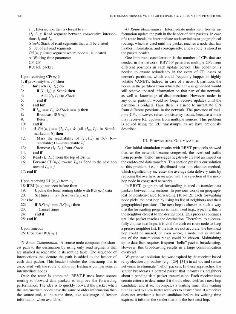
TABLE IISIMULATION SETUP

segment on the map. We also specified traffic-light-operated in-tersections and priority intersections (i.e., less than one-fifth ofthe intersections are regulated using traffic lights). We discardthe first 2000 s of the SUMO output to obtain more accuratenode movements. The output from SUMO is converted intoinput files for the movement of nodes in the NS-2 simulator.

For the wireless configuration, we used the IEEE 802.11with DCF standard [22] at the MAC layer. At the physicallayer, we used the shadowing propagation model to characterizephysical propagation. We set a communication range of 400 mwith an 80% probability of success for transmissions. Thesevalues were selected based on studies (e.g., [37]) that reportedreal-life measurements between moving vehicles in the range450–550 m. In addition, although the DSRC standard specifiesa range of up to 1000 m for safety applications, many nonsafetyapplications are expected to reach 400 m [23]. The values ofpath loss exponent β = 3.25 and deviation σ = 4.0 are usedfor the shadowing propagation [35].

We simulate buildings in a city environment using the fol-lowing obstacle model. The contour of each street can either bea building wall (of various materials) or an empty area. Thus,for each street border, we set a signal attenuation value thatwas randomly selected between 0 and 16 dB. This attenuationis added to the signal attenuation that was determined by theshadowing propagation model in NS2. We found that the signalattenuation values that were obtained were comparable withvalues reported from field experiments at 5.3 GHz [38]. Thesimulation parameters are summarized in Table II.

We ran experiments in networks with different node den-sities: 1) the 350-node scenario represents relatively densenetworks, 2) the 250-node scenario represents medium-densitynetworks, and 3) the 150-node scenario represents sparse net-works. The implementation of AODV was provided by NS-2.30(with link-layer feedback being enabled), whereas the imple-mentation of GSR is based on [6]. The GPSR implementationcode is taken from [39], and the OLSR implementation codeis taken from [40]. To allow the vehicle nodes to have moreaccurate neighbor information, we set the hello interval to0.8 s and purge neighbors from the cache after 1.6 s of inac-tivity. The topology control interval in OLSR was set to 2 s.

2) Simulation Results:Average delivery ratio: Fig. 10 shows that RBVT-R out-

performs the other protocols, with as much as a 40% increasecompared with AODV and as much as 30% increase comparedwith GSR. For most cases, we observe a decrease in the averagedelivery ratio as the data traffic increases. The descending slope

Fig. 10. Average delivery ratio for RBVT-R, RBVT-P, AODV, OLSR, GPSR,and GSR in networks with 15 flows and different node densities. (a) Onehundred fifty nodes. (b) Two hundred fifty nodes. (c) Three hundred fifty nodes.

is not acute, which means that the protocols can cope withthe offered load. This result is partly due to the presence ofobstacles on the map area, which limit the level of contentionin the wireless network. RBVT-P performs better in mediumand dense networks than in sparse networks. The reason is that,when the density is small [see Fig. 10(a)], network partitionsprevent the CPs from covering large sections of the map, thuslimiting the information gathered by the CPs.

Across network densities, we observe that the delivery ratioof protocols that integrate road layouts (i.e., RBVT protocols


and GSR) increases as the network becomes denser. BothRBVT protocols perform better than GSR for all the densities,because they integrate real-time knowledge of the vehiculartraffic on the roads. When the network is sparse, GSR does notperform as well as some node-centric protocols [see Fig. 10(a)].However, as the node density increases, the shortest path alongthe roads map becomes more likely to have enough nodes; thus,there is an increase in the average delivery ratio.

Higher node densities do not necessarily mean improvedperformances for protocols that do not consider the road lay-outs. For example, in OLSR, the increase in the number ofnodes translates into an increase of the link state updates. Twoobservations can be made on GPSR. First, given that city roadsinclude irregularities such as dead-end streets, following theshortest Euclidean distance is not always equivalent to follow-ing the shortest path through the roads. Second, the GPSRprotocol is stateless, and this condition generally providesmany advantages for the routing of data packets. However, ifa local maxima forms in the network, the stateless nature of theprotocol means that packets will follow the same path to theposition of the local maxima, and once there, the forwardingmode of each packet will be set to perimeter forwarding. Thiscase is unlike protocols that implement feedback mechanisms,e.g., AODV, which can perform a local repair or send a routeerror notification to the data source node.

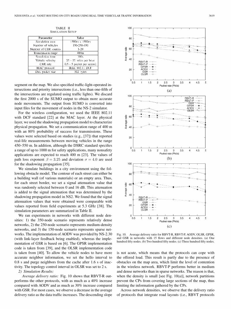
Average delay: Fig. 11 shows that RBVT-P has the small-est average delay among the protocols studied. RBVT-P per-forms better than RBVT-R due to the proactive-versus-reactivenature of the two protocols. In RBVT-P, the routes already existduring data transmission, whereas in RBVT-R, RD processesare started. Furthermore, the cost of gathering and dissemi-nating routes in RBVT-P is shared among all the data flows,whereas in RBVT-R, each new flow adds its own routing cost.Thus, unlike in MANETs, proactive road-based protocols withreal-time traffic awareness can be a viable approach in vehicularnetworks, particularly for delay sensitive applications such asvideo streaming.

We also observe that the average delay for RBVT-P con-sistently remains less than 1 s, whereas the average delay ofRBVT-R decreases with the increase in density. The reasonfor this case is that RBVT-R routes remain active for longerperiods of time (as the number of nodes increases). Thus, fewerpackets need to be buffered, because the source repairs theroute. The average delay of GSR, on the other hand, continuallyincreases, because GSR forwards data on road segments thatwere solely selected based on the positions of the communi-cation endpoints. A side effect to this step is that some roadsegments may become congested; however, because there isno communication quality feedback that is sent back to thesource vehicle, the overall communication performance suffers.This result suggests that altering the paths used in GSR byusing feedback from the network may improve the protocolperformances.

Average path length: Fig. 12(a) plots the average pathlength of packets that were received at the destination for theprotocols. This plot is similar for different network densities,and we only present the results with 250 nodes. RBVT-R haslonger average paths than the other protocols. There are two

Fig. 11. Average delay for RBVT-R, RBVT-P, AODV, OLSR, GPSR, andGSR in networks with 15 flows and different node densities. (a) One hundredfifty nodes. (b) Two hundred fifty nodes. (c) Three hundred fifty nodes.

reasons for this result: 1) RBVT-R gives preference to linkquality over forward progress when selecting the next neighbornode, and 2) unlike RBVT-P, which consistently selects theshortest connected path, a route that was established withRBVT-R is used until the source considers it broken, even ifshorter routes form at a later time. This case suggests thatRBVT-R can benefit from a method of assessing the qualityof the routes used for communications, even when they arenot broken. In addition, we note that longer path lengths donot necessarily translate, as could be expected, into worseperformance. On the contrary, selecting better forwarding nodes


Fig. 12. (a) Average path length for variable data-sending rates and(b) average delivery ratio with a variable number of concurrent flows. The datarate in (b) is fixed at 4 packets/s, and the network size is 250 nodes.

leads to better performance (e.g., RBVT-R has the highestdelivery ratio despite having longer paths).

Impact of the number of flows: The impact of the numberof concurrent flows on the protocols’ performance is shownin Fig. 12(b). The packet sending rate is 4 packets/s. RBVTprotocols perform best in terms of delivery ratio. We observethat all the protocols scale well with the increase in the numberof CBR flows in this scenario. The drop in performance issmall, i.e., from 1 to 20 CBR pairs. All protocols that we haveconsidered sustained sufficient multiple concurrent flows. Wealso compared running M flows with data rate N packet/sversus running N flows with data rate M packet/s. We observedthat the performance is slightly better when we have more flows(and lower data rates per flow) because the traffic is more evenlydistributed across the network.

D. Simulation Results in the Scenario Without Obstacles

1) Simulation Setup: Our second simulation scenario usesa 1500 m × 1500 m area that was extracted from theTIGER/Line database of the U.S. Census Bureau [21], whichforms a grid layout with a total of 22 road segments. It isan area of Fellsmere, FL, with center point coordinates lati-tude 27.784728◦ North and longitude −80.604385◦ West. Weset bidirectional traffic on each road, with two lanes in eachdirection. To evaluate the protocols under increased networkcongestion, we do not include obstacles in this scenario. This

way, a small increase in the data-sending rate will provide anoticeable increase in the level of contention in the network.

We generate the vehicle movements using a microscopicmobility generator that we have developed based on the car-following and lane-changing models proposed by Gipps [19],[20]. The Gipps model belongs to the class of collision-avoidance vehicular mobility models. The main goal of thesemodels is to allow a vehicle to move at the maximum safestspeed that avoids collisions with the preceding vehicle. Wetarget city scenarios; thus, our generator supports traffic lights atroad intersections, as well as bidirectional and multilane traffic.The input to the generator is a map of the roads with specifica-tions of the average speed and the average traffic flow on eachroad. When a vehicle enters a road segment, we determine itsaction at the end of the segment (i.e., left turn, right turn, u turn,or straight ahead) based on the average traffic flows of the roadscrossing the end intersection. We discard the first 2000 s of theoutput to obtain more accurate movements of nodes.

We used the IEEE 802.11 with DCF standard for AODV,OLSR, GPSR, and GSR, and the forwarding optimizations forthe RBVT protocols. We set the “hello” interval to 2 s, becauseit provided better results in this scenario. At the physical layer,we used the shadowing propagation model to characterize phys-ical propagation. For these simulations, the wireless range is setto 250 m to prevent communication between vehicles on paral-lel streets (the minimum distance between streets is 400 m).In the simulations, we set the exponents for the waiting func-tion in the next-hop self-election mechanism to α1 = 0.07,α2 = 0.5, and α3 = 0.03. We use the last-in–first-out (LIFO)queuing instead of the first-in–first-out (FIFO) queuing forRBVT in this scenario because it provided better latency whenexperiencing high contention [41].

2) Simulation Results:Average delivery ratio: Fig. 13 shows that the RBVT

protocols outperform the other protocols. We note that all theprotocols are more sensible to the increase in the data rate. BothRBVT protocols perform better than the other protocols underadded congestion because of the forwarding optimization. At3 packet/s, for example, only RBVT-R and RBVT-P have a datadelivery ratio above 50%. Comparing RBVT-P with OLSR, weobserve that OLSR performance is more affected by contentionin the network. RBVT-P maintains only the overall connectivitybetween the road intersections in the network, whereas OLSRproactively maintains the link state between the multipointrelays.

Average delay: Fig. 13(b) shows that, for most packetrates, RBVT-P has the best performance in terms of delay.The contention on the wireless channel can clearly be observedhere, with the values of the average delay for GPSR and GSRincreasing well above 5 s.

Impact of number of flows: The impact of the number ofconcurrent flows on the protocol performances in this scenariois shown in Fig. 14. In general, the fewer the number of flows,the better the protocol performance in terms of delivery ratio.Among the protocols, the RBVT protocols scale better thanthe other protocols. AODV shows the most accentuated drop indelivery ratio, with a 50% decrease from the 1-flow simulationto the 20-flow simulation. AODV protocol can keep the average


Fig. 13. Average delivery ratio and average delay for RBVT-R, RBVT-P, AODV, OLSR, GPSR, and GSR in networks under high contention. (a) Average deliveryratio over 250 nodes. (b) Average delay over 250 nodes.

Fig. 14. Average delivery ratio and average delay with varying numbers of concurrent flows. The data rate is fixed at 4 packets/s, and the network size is250 nodes. (a) Average delivery ratio. (b) Average delay.

delay of the transmitted data in check by dropping packets forwhich it does not have a route. GSR does not scale very wellwith the variation in the number of flows either, particularlyfor the delay that practically doubles for 20 flows comparedwith one flow. RBVT-R has the minimum decrease in deliveryratio among the simulated protocols [see Fig. 14(a)]. However,RBVT-R’s average delay is more sensitive to the added flowsthan RBVT-P’s, which consistently maintains a small averagedelay.

Overhead: As expected, based on the results in Table I,the next-hop self election mostly eliminates the overhead ofthe RBVT protocols compared with other protocols such asAODV and GSR. Although RBVT-R floods RD requests andRBVT-P floods the routing update packets, these overheadsare very small compared with the overhead introduced byfrequent route errors in AODV and the “hello” packets overheadin GSR. Using the roads layout and the real-time vehiculartraffic information leads to more stable paths and, hence, loweroverhead for RBVT protocols.

E. Simulation Results of Forwarding Optimization

Figs. 15 and 16 assess the impact on performance of theproposed geographical forwarding mechanism, which takes

advantage of the 802.11 RTS/CTS to choose the next hop usingreceiver self election, compared with a traditional approach thatuses “hello” packets to create the list of neighbors at nodes. Weconsider both scenarios with and without obstacles and bothRBVT protocols. For brevity, we show RBVT-R results usingthe map without obstacles and RBVT-P results using the mapwith obstacles.

In the scenario without obstacles, the “hello” packets weregenerated every 2 s. Fig. 15(a) shows that the forwardingoptimization leads to a delivery ratio as much as three timeshigher in congested environments. Similarly, Fig. 15(b) showsthat the delay is three times lower, on the average, with theimprovements. There are two reasons for these high improve-ments. First, the absence of periodic hello messages meansless overhead in the network. This overhead reduction leads tomuch higher link utilization for data transfers. It also leads toimproved delays, because fewer retransmissions and exponen-tial backoffs are necessary. Second, the multicriterion waitingfunction that was used in the election of the next hop favorslink quality over greediness, as explained in Section III-C.

In the scenario with obstacles [see Fig. 16(a)], the forwardingoptimizations lead to an increase in the packet delivery ratioof up 14%. The difference between the self-election and theselection results in this scenario is smaller compared with the


Fig. 15. Average delivery ratio and average delay comparison between two types of geographical forwarding, source selection using “hello” packets, and receiverself-election using our RTS/CTS-based mechanism under the scenario without obstacles. The routing protocol is RBVT-R, and the network size is 250 nodes.(a) Average delivery ratio. (b) Average delay.

Fig. 16. Average delivery ratio and average delay comparison between two types of geographical forwarding, source selection using “hello” packets, andreceiver self-election using our RTS/CTS-based mechanism under the scenario with obstacles. The routing protocol is RBVT-P, and the network size is 250 nodes.(a) Average delivery ratio. (b) Average delay.

scenario without obstacles [see Fig. 15(a)]. This result is dueto the reduced level in contention because of the obstacles. Theaverage delay is also reduced.

F. Simulation Results of RBVT-P CPs

In our final simulations, we analyze the parameters thatinfluence the accuracy of the connectivity view of the nodesin RBVT-P: 1) the number of CPs generated per period; 2) thegeographical dispersion of the CP initiators; and 3) the intervalbetween generation of CPs. For this study, we employ thescenario with obstacle and the IEEE 802.11 DCF standard atthe MAC layer. Unless otherwise specified, we used 250 nodesin the simulations, and the CP interval was set at 10 s. Anode generates a CP after the following instances: 1) It verifiesthat it has not received any CP update for a period that is atleast equal to the CP interval, and 2) it executes a Booleanfunction, for which the return value is determined based on thenumber of desired CPs. We measure the percentage of falsenegatives between pairs of vehicle nodes, i.e., the differencebetween the nodes’ local connectivity view and the simulatorglobal connectivity view for every pair of nodes in the network.

1) Number of CPs: To understand the impact of the numberof generated CPs on the accuracy of the connectivity map, weran simulations with different numbers of CPs. In this test, thenodes that generate the CPs were randomly selected, regardlessof their relative positions on the map.

TABLE IIIFALSE NEGATIVES WITH THE NUMBER OF CPS

Table III shows that, as the number of CPs generated in thenetwork increases, the number of false-negative informationbetween vehicle pairs substantially decreases. Considering thatthere is a tradeoff between a complete real-time view and theamount of CPs that would be required to generate it, we selectthree CPs as a good tradeoff between accuracy and overheadfor this map size and features.

2) Interval Between CP Generation: Next, we assess theimpact of the CP interval (i.e., the time between the generationof new CPs in the network). Five vehicles are randomly selectedto create CPs, and the number of vehicle nodes is 350.

The percentage of false negatives was 47.60% when theinterval between CP was 5 s and 9.13% when the intervalbetween CP was 10 s. One would have expected that a lower CPgeneration interval would lead to better results. However, this isnot the case, because it also leads to higher overhead, which, inturn, leads to more packet drops. The significant difference be-tween 5and 10-s intervals suggests that an inadequate selectionof this parameter can adversely affect the RBVT-P protocol’sperformance.

3) Distribution of CP Generator: Our final test assesses theinfluence of the geographical distribution of the CP initiators


TABLE IVFALSE NEGATIVES AND THE POSITIONS OF CP INITIATORS

on the accuracy of the connectivity information. For this test,we position three static vehicles at specific positions in the maparea. In the “Near” case, the vehicles are positioned close to oneanother, and in the “Spread” case, the vehicles are spread on themap area.

As expected, Table IV shows that, when the CP initiators arespread on the map, the quality of the connectivity informationimproves. The fact that the vehicles used in the “Spread”simulation were not moving does not seem to have a noticeableimpact. Its results are comparable with those in Table III, wheremoving vehicles were used.

V. RELATED WORK

Routing has been a major research topic in MANETs. AODV[8], DSDV [42], DSR [9], and OLSR [28] are node-centricMANET protocols in which topological end-to-end paths arecreated. To improve on their performance in VANETs, solutionshave been proposed, which exploit the knowledge of relativevelocities between nodes and the constrained movements ofvehicles [43]–[45]. This information is used to select nodeswith high relative velocity to the destination, predict the lifetimeof routes, or reduce the number of route breaks by selecting,during the route creation, nodes that move in the same directionand with a small relative speed. RBVT routing differs fromthese protocols in that the routes are road based, and their maincomponents are the road intersections that were traversed on thepath from the source to the destination.

Geographical routing protocols, e.g., GPSR [12], GFG [10],and GOAFR [11], use node positions to route data betweenendpoints. When a local maxima is reached (i.e., a positionwhere progress cannot be made based on node positions),recovery strategies are proposed to route the packets around thevoid. Solutions in [46] and [47] propose to improve recoverystrategies in VANETs by either proactively detecting potentialdead-end positions or using channel overhearing capabilitiesof wireless networks to decrease the number of hops on therecovery paths.

The concept of anchor-based routing in sensor networks [48],[49] has been adopted to VANET environments. GSR [6] andSAR [14] integrate the road topologies in routing using thoseconcepts. In these protocols, a source computes the shortestroad-based path from its current position to the destination.Similar to RBVT, they include the list of intersections thatdefine the path from the source to the destination in the headerof each data packet that was sent by the source. However,they do not consider the real-time vehicular traffic, and con-sequently, they could include empty roads. To alleviate thisissue, A-STAR [50] modifies GSR by giving preference tostreets served by transit buses each time a new intersection willbe added to the source route. CAR [7] finds connected pathsbetween source–destination pairs, considering vehicular traffic,and uses “guards” to adapt to movements of nodes. Gytar [15]

dynamically adds intersections, choosing the next road segmentwith the best balance of road density and road length.

MDDV [17] and VADD [16] use opportunistic forwarding totransport data from the source to the destination in VANETs.VADD uses historic data traffic flow to determine the best routeto the destination. MDDV considers the road traffic conditionsand the number of lanes on each road segment to select the bestroad-based trajectory to forward data. In both protocols, whenno vehicle node can be found along the forwarding trajectory, acarry-and-forward approach is used, and the data packets arestored until a more suitable relay is found. These protocolsare well suited for delay-tolerant applications (i.e., applicationsfor which the users can tolerate a certain level of delay, aslong as the data eventually arrives). A delay-tolerant epidemicrouting approach for VANETs is presented in [51]. Under verysparse vehicular traffic and at the early stages of the deploymentof wireless technology in vehicles (when many vehicles willnot have wireless interfaces), such opportunistic forwardingsolutions will be useful to car-to-car ad hoc communications.The RBVT protocols, on the other hand, provide support forapplications that are not necessarily delay tolerant. RBVTprotocols require that an end-to-end path exists for data to reachthe destination.

Receiver-based next-hop selection is proposed at the routinglayer (e.g., [29]) and at the MAC layer (e.g., [30]–[34]). In[29], all neighbors receive the entire packet, but only oneneighbor will rebroadcast it. This neighbor is the one that winsa time-based contention phase in which the node closest to thedestination is favored. Minimizing the remaining distance to thedestination is also the objective in [30], [31], and [34], whichoperate at the MAC layer. These methods consider the unit-diskassumption, which does not hold in real-life VANETs. RBVTnext-hop self election can work in realistic conditions, whereobstacles and noise frequently affect wireless communication,because it incorporates multiple criteria in the selection of thebest next hop (i.e., forwarding progress, optimal transmissionarea, and received power).

Multicriterion receiver-based next-hop selection has beendescribed in a general form in [33]. The authors demonstratedthat using carefully selected criteria can improve the election ofthe optimal next hop. We apply these results in the context ofvehicular networks and define a set of criteria to optimize theelection of the next hop.

We note that real-life measurements with commercial GPSreceivers [52] showed errors in the reporting of GPS positionsin urban environments. RBVT protocols follow paths made ofroad segments; thus, they are more resilient to vehicle nodeposition errors of a few meters. The integration of the inertialnavigation system into GPS receivers is expected to improvethe detection and handling of GPS position errors.

VI. CONCLUSION

This paper has presented RBVT, which is a class of VANETrouting protocols for city-based environments that takes advan-tage of the layout of the roads to improve the performanceof routing in VANETs. RBVT protocols use real-time vehic-ular traffic information to create road-based paths between


endpoints. Geographical forwarding was used to find forward-ing nodes along the road segments that form these paths. Toimprove the end-to-end performance under high contention, wehave also proposed a distributed next-hop self-election mech-anism for geographical forwarding. Simulation results haveshown that our two protocols, namely RBVT-R and RBVT-P, outperform existing approaches in terms of the averagedelivery ratio and average delay. The RBVT protocols forwarddata along the streets (not across the streets) and take thereal traffic on the roads into account; thus, they perform wellin realistic vehicular environments in which buildings andother road characteristics, e.g., dead-end streets, are present.These results show that distributed applications that generatea moderate amount of traffic can successfully be implementedin VANETs. Furthermore, these applications can use RBVT-Rwhen throughput is their main requirement and RBVT-P if theyare delay sensitive.

REFERENCES

[1] S. Dashtinezhad, T. Nadeem, B. Dorohonceanu, C. Borcea, P. Kang, andL. Iftode, “Trafficview: A driver assistant device for traffic monitoringbased on car-to-car communication,” in Proc. 59th IEEE Semiannual Veh.Technol. Conf., Milan, Italy, May 2004, pp. 2946–2950.

[2] P. Zhou, T. Nadeem, P. Kang, C. Borcea, and L. Iftode, “EZCab: A cabbooking application using short-range wireless communication,” in Proc.3rd IEEE Int. Conf. PerCom, Kauai Island, HI, Mar. 2005, pp. 27–38.

[3] O. Riva, T. Nadeem, C. Borcea, and L. Iftode, “Context-aware migratoryservices in ad hoc networks,” IEEE Trans. Mobile Comput., vol. 6, no. 12,pp. 1313–1328, Dec. 2007.

[4] A. Nandan, S. Das, G. Pau, and M. Gerla, “Cooperative downloadingin vehicular ad hoc wireless networks,” in Proc. 2nd Annu. IEEE Conf.WONS, St. Moritz, Switzerland, Jan. 2005, pp. 32–41.

[5] CarTel, Mass. Inst. Technol., Cambridge, MA. [Online]. Available: http://cartel.csail.mit.edu

[6] C. Lochert, H. Hartenstein, J. Tian, H. Füßler, D. Hermann, andM. Mauve, “A routing strategy for vehicular ad hoc networks in cityenvironments,” in Proc. IEEE Intell. Vehicles Symp., Columbus, OH,Jun. 2003, pp. 156–161.

[7] V. Naumov and T. Gross, “Connectivity-aware routing (CAR) in ve-hicular ad hoc networks,” in Proc. IEEE Int. Conf. Comput. Commun.,Anchorage, AK, May 2007, pp. 1919–1927.

[8] C. E. Perkins and E. M. Royer, “Ad hoc on-demand distance vectorrouting,” in Proc. 2nd IEEE Workshop Mobile Comput. Syst. Appl.,New Orleans, LA, Feb. 1999, pp. 90–100.

[9] D. B. Johnson and D. A. Maltz, “Dynamic source routing in ad hocwireless networks,” Mobile Comput., vol. 353, no. 5, pp. 153–161, 1996.

[10] P. Bose, P. Morin, I. Stojmenovic, and J. Urrutia, “Routing with guar-anteed delivery in ad hoc wireless networks,” ACM Wirel. Netw., vol. 7,no. 6, pp. 609–616, Nov. 2001.

[11] F. Kuhn, R. Wattenhofer, Y. Zhang, and A. Zollinger, “Geometric ad hocrouting: Of theory and practice,” in Proc. 22nd Annu. Symp. PrinciplesDistrib. Comput., Boston, MA, Jul. 2003, pp. 63–72.

[12] B. Karp and H. T. Kung, “GPSR: Greedy perimeter stateless routingfor wireless networks,” in Proc. 6th Annu. Int. MobiCom, Boston, MA,Aug. 2000, pp. 243–254.

[13] T. Li, S. K. Hazra, and W. Seah, “A position-based routing protocol formetropolitan bus networks,” in Proc. 61st IEEE VTC—Spring, Stockholm,Sweden, Jun. 2005, pp. 2315–2319.

[14] J. Tian, L. Han, K. Rothermel, and C. Cseh, “Spatially aware packetrouting for mobile ad hoc intervehicle radio networks,” in Proc. IEEEIntell. Transp. Syst., Shanghai, China, Oct. 2003, pp. 1546–1551.

[15] M. Jerbi, R. Meraihi, S.-M. Senouci, and Y. Ghamri-Doudane, “Gytar:Improved greedy traffic aware routing protocol for vehicular ad hoc net-works in city environments,” in Proc. 3rd ACM Int. Workshop VANET,Los Angeles, CA, Sep. 2006, pp. 88–89.

[16] J. Zhao and G. Cao, “VADD: Vehicle-assisted data delivery invehicular ad hoc networks,” IEEE Trans. Veh. Technol., vol. 57, no. 3,pp. 1910–1922, May 2008.

[17] H. Wu, R. Fujimoto, R. Guensler, and M. Hunter, “MDDV: A mobility-centric data dissemination algorithm for vehicular networks,” in Proc. 1stACM Int. Workshop VANET, Philadelphia, PA, Oct. 2004, pp. 47–56.

[18] Centre for Applied Informatics (ZAIK) and the Institute of Trans-port Research German Aerospace Centre, Sumo—Simulation of UrbanMobility (last accessed Jul. 2008). [Online]. Available: http://sumo.sourceforge.net/

[19] P. G. Gipps, “A behavioral car-following model for computer simulation,”Trans. Res. Board, vol. 15, no. 2, pp. 105–111, Apr. 1981.

[20] P. Gipps, “A model for the structure of lane-changing decisions,” Trans.Res. Board, vol. 20B, no. 5, pp. 403–414, Oct. 1986.

[21] U.S.Census Bureau—TIGER/Line 2006 Second ed. (last accessedJul. 2008). [Online]. Available: http://www.census.gov/geo/www/tiger/

[22] Institute of Electrical and Electronic Engineers (IEEE), WirelessLAN Medium Access Control (MAC) and Physical Layer Specifications.[Online]. Available: http://standards.ieee.org/getieee802/802.11.html

[23] “Task 3 Final Report,” Identify Intelligent Vehicle Safety Applica-tions Enabled by DSRC, DOT HS 809 859, Mar. 2005 (last accessedJul. 2008). [Online]. Available: http://www-nrd.nhtsa.dot.gov/pdf/nrd-12/1665CAMP3web/index.html

[24] S.-Y. Ni, Y.-C. Tseng, Y.-S. Chen, and J.-P. Sheu, “The broadcast stormproblem in a mobile ad hoc network,” in Proc. 5th Annu. ACM/IEEE Int.Conf. Mobile Comput. Netw., Seattle, WA, Aug. 1999, pp. 151–162.

[25] L. Briesemeister and G. Hommel, “Role-based multicast in highly mobilebut sparsely connected ad hoc networks,” in Proc. 1st Annu. WorkshopMOBIHOC, Boston, MA, Aug. 2000, pp. 45–50.

[26] Q. Sun, S. Y. Tan, and K. C. Teh, “Analytical formulae for path lossprediction in urban street grid microcellular environments,” IEEE Trans.Veh. Technol., vol. 54, no. 4, pp. 1251–1258, Jul. 2005.

[27] J. Li, J. Jannotti, D. S. J. De Couto, D. R. Karger, and R. Morris, “Ascalable location service for geographic ad hoc routing,” in Proc. 6thACM Int. Conf. MobiCom, Boston, MA, Aug. 2000, pp. 120–130.

[28] T. Clausen and P. Jacquet, Optimized Link State Routing Protocol (OLSR),2003. [Online]. Available: http://hipercom.inria.fr/olsr/rfc3626.txt

[29] H. Füßler, J. Widmer, M. Käsemann, M. Mauve, and H. Hartenstein,“Contention-based forwarding for mobile ad hoc networks,” Ad HocNetw., vol. 1, no. 4, pp. 351–369, Nov. 2003.

[30] K. Egoh and S. De, “Priority-based receiver-side relay election in wirelessad hoc sensors networks,” in Proc. Int. Conf. Wireless Commun. MobileComput., Vancouver, BC, Canada, Jul. 2006, pp. 1177–1182.

[31] M. Chawla, N. Goel, K. Kalaichelvan, A. Nayak, and I. Stojmenovic,“Beaconless position-based routing with guaranteed delivery for wire-less ad hoc and sensor networks,” Acta Autom. Sin., vol. 32, no. 6,pp. 847–855, Nov. 2006.

[32] G. Zhou, T. He, S. Krishnamurthy, and J. A. Stankovic, “Impact ofradio irregularity on wireless sensor networks,” in Proc. 2nd Int. Conf.MOBISYS, Boston, MA, Jun. 2004, pp. 125–138.

[33] K. Egoh and S. De, “A multicriteria receiverside relay election approachin wireless ad hoc networks,” in Proc. MILCOM, Washington, DC,Oct. 2006, pp. 1–7.

[34] M. Zorzi and R. R. Rao, “Geographic random forwarding (GERAF) forad hoc and sensor networks: Multihop performance,” IEEE Trans. MobileComput., vol. 2, no. 4, pp. 337–348, Oct.–Dec. 2003.

[35] T. S. Rappaport, Wireless Communications Principles and Practice.Englewood Cliffs, NJ: Prentice–Hall, 1996.

[36] The Network Simulator: NS-2. [Online]. Available: http://www.isi.edu/nsnam/ns

[37] N. Eude, B. Ducourthial, and M. Shawky, “Enhancing ns-2 simulator forhigh mobility ad hoc networks in car-to-car communication,” in Proc. 7thIFIP Int. Conf. Mobile Wireless Commun. Netw., Marrakech, Morocco,Sep. 2005.

[38] X. Zhao, T. Rautiainen, K. Kalliola, and P. Vainikainen, “Path-loss modelsfor urban microcells at 5.3 GHz,” IEEE Antennas Wireless Propag. Lett.,vol. 5, no. 1, pp. 152–154, Dec. 2006.

[39] B. Karp, Greedy Perimeter Stateless Routing (GPSR) (last accessedJul. 2008). [Online]. Available: http://www.icir.org/bkarp/gpsr/gpsr.html

[40] HIPERCOM, INRIA, Optimized Link State Routing Protocol (OLSR) (lastaccessed Jul. 2008). [Online]. Available: http://hipercom.inria.fr/olsr/

[41] J. Nzouonta, T. Ott, and C. Borcea, Impact of Queue Discipline onStreaming Latency in Ad Hoc Networks, submitted for publication.

[42] C. E. Perkins and P. Bhagwat, “Highly dynamic destination-sequenceddistance-vector routing (DSDV) for mobile computers,” in Proc. ACMSIGCOMM Conf. Commun. Architectures, Protocols Appl., London, U.K.,Sep. 1994, pp. 234–244.

[43] K.-T. Feng, C.-H. Hsu, and T.-E. Lu, “Velocity-assisted predictive mo-bility and location-aware routing protocols for mobile ad hoc networks,”IEEE Trans. Veh. Technol., vol. 57, no. 1, pp. 448–464, Jan. 2008.

[44] V. Namboodiri and L. Gao, “Prediction-based routing for vehicular ad hocnetworks,” IEEE Trans. Veh. Technol., vol. 56, no. 4, pp. 2332–2345,Jul. 2007.


[45] T. Taleb, E. Sakhaee, A. Jamalipour, K. Hashimoto, N. Kato, andY. Nemoto, “A stable routing protocol to support its services inVANETs,” IEEE Trans. Veh. Technol., vol. 56, no. 6, pp. 3337–3347,Nov. 2007.

[46] C.-H. Chou, K.-F. Ssu, and H. C. Jiau, “Geographic forwarding with dead-end reduction in mobile ad hoc networks,” IEEE Trans. Veh. Technol.,vol. 57, no. 4, pp. 2375–2386, Jul. 2008.

[47] X. Ma, M.-T. Sun, G. Zhao, and X. Liu, “An effïcient path pruningalgorithm for geographical routing in wireless networks,” IEEE Trans.Veh. Technol., vol. 57, no. 4, pp. 2474–2488, Jul. 2008.

[48] L. Blazevic, L. Buttyan, S. Capkun, S. Giordano, J.-P. Hubaux, andJ.-Y. L. Boudec, “Self-organization in mobile ad hoc networks:The approach of terminodes,” IEEE Commun. Mag., vol. 39, no. 6,pp. 166–174, Jun. 2001.

[49] L. Blazevic, S. Giordano, and J.-Y.-Y. L. Boudec, “Self-organized termin-ode routing,” J. Cluster Comput., vol. 5, no. 2, pp. 205–218, Apr. 2002.

[50] B.-C. Seet, G. Liu, B.-S. Lee, C.-H. Foh, K.-J. Wong, and K.-K. Lee,“A-star: A mobile ad hoc routing strategy for metropolis vehicularcommunications,” in Proc. NETWORKING, Apr. 2004, vol. 3042,pp. 989–999.

[51] H.-Y. Huang, P.-E. Luo, M. Li, D. Li, X. Li, W. Shu, and M.-Y. Wu,“Performance evaluation of SUVnet with real-time traffic data,” IEEETrans. Veh. Technol., vol. 56, no. 6, pp. 3381–3396, Nov. 2007.

[52] S. Savasta, M. Pini, and G. Marfia, “Performance assessment of a com-mercial GPS receiver for networking applications,” in Proc. IEEE Int.Consumer Commun. Netw. Conf., Las Vegas, NV, Jan. 2008, pp. 613–617.

Josiane Nzouonta received the M.S. degree in com-puter science from the Florida Institute of Technol-ogy, Melbourne, in 2003. She is currently pursuingthe Ph.D. degree with the Department of Com-puter Science, New Jersey Institute of Technology,Newark.

Her research interests include wireless ad hocnetworks, vehicular networks, and security in distrib-uted systems.

Neeraj Rajgure received the M.S. degree in com-puter science from the New Jersey Institute ofTechnology (NJIT), Newark, in 2008.

His research interests include wireless sensor net-works and vehicular networks.

Guiling (Grace) Wang (M’06) received the B.S.degree from Nankai University, Tianjin, China, andthe Ph.D. degree in computer science and engineer-ing, with a minor in statistics, from the PennsylvaniaState University, University Park, in 2006.

She is currently an Assistant Professor with theDepartment of Computer Science, New Jersey Insti-tute of Technology, Newark. Her research interestsinclude distributed systems, wireless networks, andmobile computing, with emphasis on wireless sensornetworks.

Cristian Borcea (M’02) received the Ph.D. de-gree in computer science from Rutgers University,Piscataway, NJ, in 2004.

He is currently an Assistant Professor with theDepartment of Computer Science, New Jersey Insti-tute of Technology, Newark. His research interestsinclude mobile computing, middleware, ad hoc net-works, and distributed systems.

Dr. Borcea is a member of the Association forComputing Machinery and the Advanced Comput-ing Systems Professional and Technical Association

(Usenix).

vanet routing on city roads using real-time vehicular ... · nzouonta et al.: vanet routing on city...

Documents