var-methodology in risk managment · var-methodology in risk-management of the bank’s interest...
TRANSCRIPT
VAR-METHODOLOGY IN RISK-MANAGEMENT OF THE BANK’S
INTEREST RATE AND EXCHANGE RATE: IS IT
POSSIBLE, USEFUL AND VALID IN THE UKRAINIAN BANK
MARKET?
by
Olha Venchak
A thesis submitted in partial fulfillment of the requirements for the
degree of
Master of Arts in Economics
National University “Kyiv-Mohyla Academy” Economics Education and Research Consortium
Master’s Program in Economics
2005
Approved by ___________________________________________________ Ms. Svitlana Budagovska (Head of the State Examination Committee)
__________________________________________________
__________________________________________________
__________________________________________________
Program Authorized to Offer Degree Master’s Program in Economics
Date _________________________________________________________

National University of “Kyiv-Mohyla Academy”
Abstract
VAR-METHODOLOGY IN RISK-MANAGEMENT OF THE BANK’S
INTEREST RATE AND EXCHANGE RATE: IS IT POSSIBLE, USEFUL AND VALID IN
THE UKRAINIAN BANK MARKET?
by Olha Venchak
Head of State Examination Committee: Ms. Svitlana Budagovska, Economist, World Bank of Ukraine
This thesis is devoted to risk-management in Ukrainian banks. Value-at-Risk
methodology, which is widely used in developed countries, is not popular
among Ukrainian risk-managers. The main stone on the road was the
transition conditions inside the country, which disturbs market mechanisms.
Today the situation is changed!
On the example of one of Ukrainian commercial banks “Kredyt-Bank
(Ukraine)” I applied VaR to calculating exchange rate risk and interest rate
risk. In calculating exchange rate risk I used untraditional approach.
Simulations in VaR for both kinds of risk were made by standard (variance-
covariance) and historical simulations methods. Results, which I got, are very
useful for planning the stable, profitable and prosperous future of the bank.
By Basel Committee (2004), banks that want to cooperate on the open
financial market and to be a strong competitor to developed banks must use
in its risk-management VaR methodology.
It is the time to be on the same level with leading countries!

TABLE OF CONTENTS
List of Figures and Tables..................................................................................ii
List of Appendix Figures and Tables.................................................................iii Acknowledgements...........................................................................................iv Glossary ............................................................................................................v Chapter1. INTRODUCTION..........................................................................1 Chapter 2. Literature Review..............................................................................6 2.1 History of Risk Management..................................................................6 2.2 Risk Classification .................................................................................8 2.3 Basel Committee and Value-at-Risk......................................................10 2.4 Value-at-Risk Classification and Methodologies....................................11 Chapter 3. Methodology ..................................................................................19 3.1 Classical VaR Computation..................................................................19 3.2 Parametric and Non-Parametric Approaches to VaR.............................21 3.2 Method of Historical Simulations..........................................................22 3.3 Delta-Normal Method (variance-Covariance Method)...........................24 3.4 Calculation of the Exchange Rate risk Through VaR.............................25 3.5 Similar method to VaR, Based on the Historical Simulations And on the Delta-Normal Simulations..........................................................................27 3.6 Back-Testing .........................................................................................31 Chapter 4. Data Description.............................................................................34 Chapter 5. Estimated Results............................................................................36 5.1 Back-testing.........................................................................................36 5.2. Value-at-Risk, Interest Rates Deviations...............................................38 4.3. Value-at-Risk , Exchange Rate Deviations............................................41 Chapter 6. Implications....................................................................................43 Chapter 6. Conclusions....................................................................................46 BIBLIOGRAPHY...........................................................................................48 Appendix.........................................................................................................49

ii
LIST OF FIGURES AND TABLES
Number Figures Page Figure 1. Normality of Distribution of Deposits from Individuals Up To 1 Month .............................................................................................................22 Figure 2. Dependence of PV and Interest Rate ...............................................29 Figure 3. Back-testing: Credits for Individuals Up To 1 Month .......................37 Figure 4. Back-Testing: Deposits from Individuals Up To 12 Month ..............37 Figure 5. Back-Testing: EUR/UAH Exchange Rate .......................................38 Tables
Table 1. Types of Errors According to Type of Decision..................................32 Table 2. Basel Committee Requirements to Exceptions ....................................32 Table 3. VaR for the Credits to the Firms.........................................................40

iii
LIST OF APPENDIX FIGURES AND TABLES
Number Page Figures
Figure A1. Back-Testing for the Exchange Rate Risk........................................49 Figure A2. Back-Testing for the Interest Rate Risk, UAH.................................51 Figure A3. Back-Testing for the Interest Rate Risk, EUR..................................52 Figure A4. Back-Testing for the Interest Rate Risk, USD..................................53 Tables
Table A1. Summary Statistics for Exchange Rates ............................................54 Table A2. Assessment of Parametric and Non-Parametric VaR Models ............56 Table A3. Results with Calculated Possible Loss According to the Interest Rate Risk.........................................................................................................58 Table A4. Results with Calculated Possible Loss According to the Interest Rate Risk.........................................................................................................70

iv
ACKNOWLEDGMENTS
I would like to express my hearty thanks to my advisor Prof. Tom Coupe for
his very helpful and careful supervision, for his friendly and wise advises
during the whole process of work on my research. I also would like to thank
Prof. Volodymyr Bilotkach and Prof. Polina Vlasenko for their thorough
reviews and valuable comments. The special sincere gratitude I would like to
give to Kredyt-Bank’s (Ukraine) Risk Manager Anton Kirkach for
competence in providing necessary information and data for my research. I
give the special thank to my fiancé Taras Bunds for his gentle support during
the difficult period of thesis writing. Also I would like to give special
gratitude to God for His help and to my family for their support and
understanding.

v
GLOSSARY
Adequacy of Capital – the possibility of bank to cover its loans with the own capital.
Future value – capital’s value after the certain period of time with the interest rate profit.
GAP-method - the difference between some group of assets with respective interest and the same group of loans with respective interest: ttt LAGAP −= , it shows positive or negative gap.
Present value - today’s value of future cash flows.
Value-at-Risk - tool for estimation the exposure to different kinds of risk, which gives the worst expected loss at a given confidence level with the probability of 95% or 99%.
C h a p t e r 1
INTRODUCTION
Each year banking sector problems attract greater attention on the
Ukrainian financial market. Today, the banking system is the main “blood
system” between borrowers and lenders; it is the way of almost all possible
business finance communications. Its solidity, stability and security show the
healthiness of the whole country’s economy.
The main issue in this sphere is the improvement of the financial
stability and increasing the bank’s financial result. “Life is risky”, everyone
knows this, and hence, one of the basic determinants which directly influence
the stability and the result, is risk. Nevertheless, in finance almost everyone
would like to benefit from taking additional risk, since every additional risk
can be rewarded by the risk premium. Where is the risk coming from? The
answer is that the risk has its origin in many sources: human-created (business
cycles, inflation, wars) and natural phenomena. It also can be created from the
long-term economic growth, technological innovations and so forth. Financial
markets cannot be completely protected against all risks (Jorion 2000).
Banking risk means the probability of loss according to the specific operation
that the credit institution is engaged in. So, the main task of risk-managers is
seeking security and maintaining the equilibrium between chances to win
(earn excess profit) and risks attached to these profits. To do this the risk-
managers should be able to identify, quantify and foresee risks.
There is a wide classification of risks. Banking risks are divided into
market risk (interest rate risk, exchange rate risk, equity risk, liquidity,
commodity risk and derivative market risk), credit risk (stock and individual)
and operational risk (human risk, process risk, external event risk, and

2
technology risk). But this classification can be flexible, every bank can decide
about its own risk classification according to the market conditions it is
working with.
Market risk is the next important group of banking risks after credit risk
and it means the possibility of a change in the economic condition of the
financial institution due to the influence of some market factors. This kind of
risk covers about 25% of risk capital in bank (Kumar 2003). He wrote:
“Market risk needs more attention in most banks, because if everything seems
under control, you’re just not going fast…”
In this thesis, I would like to pay the main attention to the risk of
interest rate and to the risk of the exchange rate, the most significant types of
market risks. The first one means the danger of possible loss because of the
volatility of market interest rates and the related change in the values of
credits, loans and their present values. The second is the probability of losing
capital due to changes in the exchange rates of foreign currency to the
domestic currency during the period from the signing of the contract to the
real transaction.
Every bank tries to hold interest rate risk under control through the
high quality of its management. Consequently, to ensure the most productive
way of managing risk, instead of dictating capital and risk-management
requirements through a uniform supervisory approach, banks are allowed by
the Basel Committee1 to use their own models and expertise for computing
the capital required and the risk value (Lucas 2001). This rule extends to all
European countries, including Ukraine, but every bank in different countries
should adjust its measures with the requirements of its Central Bank (National
Bank of Ukraine in our case). Nevertheless, during long time and till now, the
Basel Committee advises to use the Value-at-Risk (VaR) as the best method of
1Basel Committee on Banking Supervision (1988) is a Committee of banking delegated supervisory authorities, established
by the central bank Governors of the group of ten leading countries: Belgium, Canada, France, Germany, Italy, Japan, Luxembourg, Netherlands, Spain, Sweden, Switzerland, United Kingdom and the United States.
3
measuring banking risk in the money equivalent. This method predicts the
possible losses that will not exceed (1-p) %. But, in 2007, when the Basel II2
will come into effect, VaR will be not only the recommended methodology,
but also the required one for risk measuring in the accounts in those banks,
which operate on the interbank market. At that time VaR-measuring will be
obvious, but it will not forbid the parallel internal risk measuring, other than
VaR. Hence, in the nearest future the National Bank of Ukraine will also
require the VaR methodology. This information became available in the
guidelines after the Basel Committee of Banking Supervision II. Also, those
Polish professionals who already use the VaR-methodology and currently are
cooperating with Ukraine’s banking system speak about the transformation of
the standard system of our risk measuring (the largest Polish bank “PKO’’,
which cooperates with the “Kredyt-Bank (Ukraine)”).
Modern European and USA financial markets offer enough
instruments that allow full study of behavior of the interest rate and exchange
rate and provide predictability of their movement through time. My paper will
be the first attempt to describe the evaluation of the exchange rate risk
through the VaR-method for the Ukrainian banking market. It will be also the
first work in evaluating the interest rate risk through the method based on the
VaR methodology and can be considered as the similar to VaR method.
There were no attempts for measuring the interest rate risk through the
methods based on the VaR in Ukrainian banks till now. As to the exchange
rate, it is possible to calculate VaR for it, but almost no bank (the exception
are foreign banks) did this till now.
The attractiveness of VaR-methodology is in the simplicity of its idea
and realistic predictions. It makes possible to provide single statistic
estimating the potential loss to which a bank is exposed during a given period
of time with a given degree of confidence (99%) according to the type of
2 Basel II (2004) is the document (package) of recommendation for the Central Banks how to calculate the necessary
amount of capital to cover bank’s risks.

4
operation or the portfolio under some market risks. The value of VaR ensures
covering of possible losses x during time t with probability p, Pr (VaR>x) =
p. This VaR-methodology can be used for measuring different kinds of risk,
measuring all of them by this methodology makes it possible for a bank to see
the total value of capital under risk. Still banks in Ukraine did not use this
method in prediction of possible capital loss because official regulations did
not require such risk measuring. Moreover, to have the precise results of
calculating VaR the market mechanisms should work well. As far we know
market mechanisms in Ukraine are not high developed still. That is why,
market interest rate in Ukraine still have very weak correlation with the real
interest rate in Ukrainian banks.
The main condition for calculating VaR is simultaneous change of the
capital value in response to a change in some factors (e.g. the exchange rate
changes, the value of foreign capital changes too at the same time). It is
impossible to calculate the traditional VaR for the interest rate risk, because
there is no such immediate change of the capital after the change of the
market interest rate (today we have already signed contracts of deposits and
credits with adjusted interest rates). So the main investigation of this work will
be in attempt to build the method based on VaR, which will show the risk of
change the market interest rates for the present value of bank’s capital.
To use this VaR-modeling for exchange rate, I will need daily data on
exchange rates for all foreign currencies included in a bank portfolio of
foreign currencies. To apply my model, based on VaR, for calculating the
interest rate risk I will also need daily data across different interest rates:
quantity of credits and deposits of certain duration (1 month, 3 months, 6
months and so on), of certain amounts; interest rates, given by the NBU, and
the Association of the Ukrainian Banks. All of this data will be used in terms
of present values. Needed data is available from the “Kredyt-Bank (Ukraine)”,
from the NBU and from the Association of the Ukrainian Banks.
5
So, my work is an effort to use VaR methods to calculate exchange rate
and the interest rate risks, using data from one of Ukrainian commercial
banks – “Kredyt-Bank (Ukraine)” and www.finance.com. Basing on the
results, obtained after calculating VaR I will be able to answer on some next
questions. Will this methodology give us some useful results for
recommending the more likely bank credit and loan policy? What economic
meaning the calculated results will have for the bank? It will be possible to
make the conclusion about whether Ukrainian financial market and national
risk-managers are ready to follow the Basel’s requirements and work at the
same level with developed countries

6
C h a p t e r 2
LITERATURE REVIEW
2.1 History of the Risk-Measurement
Financial liberalization, intensification of the competition and the
diversification of markets create new problems for banks and good conditions
to developing of the new risks. Taking the risk upon the banks is one of the
essential principles of banking. But the banking is considered to be successful
only in the case when accepted risks are under control, if they are sensible,
under the financial abilities and jurisdiction. Achieving this goal provides the
basis of internal policy of accepting risks and managing them.
There are always a lot of problems with the aggregation and the
measuring the amount of capital under risk and the controlling of such risks
(Rogov 2001). The VaR approach, in contrast to other ones, allows the
aggregation of different risks to which bank exposures into a one amount.
According to Jorion (1997), “VaR measures the worst expected loss over a
given horizon under normal market conditions at a given level of
confidence”. Moreover, VaR method allows the comparison of different
types of risks: “Risk can only be compared when they are measured with the
same yardstick” (Morgan 1995).
The VaR methodology has been widely adopted for measuring the
market risk in bank trading portfolios among European countries and USA
during the 1990. According to Holton (2002), the beginning of VaR can be
traced back to the New York Stock Exchange in 1922 imposing the capital
requirements on the member firms. The earliest work about VaR measure
was published in 1945, when the portfolio theory was established. Probably,
7
the first VaR measure was published by Leavens (1945), when he offered the
quantitative example, discussing the portfolio construction. He did not
mention VaR, but he spoke about the “spread between probable loses and
gains”, which means the standard deviation of portfolio market value.
Nowadays, VaR is defined as a method of measuring the value of all
kinds of risk. Holton (2002) investigates the fixed holding portfolio, which
has known current market value and the future market value could be shown
as a random variable, so we can describe this methodology as a probability
function. Also we can discern the VaR metrics, as the function of the
distribution and the portfolio’s current market value (variance of return,
standard deviation and 0.95-quantile of loss) and VaR measure as any
procedure that, under a given VaR metrics, assigns values for that metrics to
portfolios.
According to Holton (2002), VaR has its roots in the portfolio theory
and capital requirements (NYSE capital requirements of the early 20-century).
In 1952, Marcowitz and later Roy independently published VaR measures.
Their works were based on selecting portfolios to optimize them for a given
level of risk. The aim of these two authors was the same – to calculate the
VaR, but the methods were different: Marcowitz used the simple return
metrics and Roy used the metric of shortfall risk that represents an upper
bound on the probability of the portfolio’s gross return, which could be less
than particular specified extreme return. In 1972, Lietar showed the practical
VaR measure for foreign exchange rate: he supposed that the depreciation
occurred randomly, its conditional magnitude being normally distributed. His
work is assumed to be the first in applying the Monte-Carlo method to the
VaR measure. During the 1970s and the 1980s markets became more volatile,
which required highest leverage and stronger financial risk measure. The
resources necessary for calculating VaR through different methods became
available in that time too. These factors stimulated VaR methodology to
improve. In that time firms demanded the way to measure the market risk

8
across the incompatible asset categories, but they did not know how VaR
might help in those problems. So US managers did a difficult work in
adopting VaR methodology for vide use (Holton 2002). During the early
1990’s the main issue in developing the VaR-methodology was concerned
with the financial risk management due to increasing number of derivative
instruments (forwards, futures, options). So far, Ukrainian risk managers do
not know precisely how to apply and explain VaR models on the Ukrainian
financial market.
The appearance of the name “value-at-risk” has a specific history too,
during 1990’s it was «dollars-at-risk» DaR, «capital-at-risk» CaR, «income-at-
risk» IaR, «earnings-at-risk» EaR and «value-at-risk» VaR. Seems that users did
not know exactly, what was “at risk” (Holton 2002).
2.2 Risk Classification
So, VaR (or similar methods) makes it possible to evaluate different
types of risk, to see the total amount of capital under risk and to compare the
value of different risks. There are different approaches in VaR-methodology,
which help to provide risk measure. Before confirming this, I will however
define the classification of banking risks (by Mandagelli, 2001):
• Credit risk relates to the potential loss due to the impossibility of the
partner to cover its duties of repaying the loan and interest. It has
three basic components: credit exposure, probability of default and
loss in the event of the default.
• Operational risk takes into account the errors and potential problems
that can be made by the banking workers or equipment in instructing
payments or setting transactions, and includes the risk of fraud and
regulatory risks.

9
• Market risk estimates the uncertainty of the future earnings due to the
changes in the market conditions; this is the risk that the value of
assets or liabilities will be affected by movements in equity and
interest rate markets, currency exchange rates and prices of the
commodities. Market risk can be divided into such main categories
(by the Basel Committee on Banking Supervision, 2004):
1. Interest rate risk is the exposure of a bank’s financial conditions
to adverse movements in interest rates. If bank accepts this
risk as a normal part of banking, it can be a huge resource of
profitability and the high value for the shareholders. Changes
in the interest rates change the net interest income, operating
expenses, which affects a bank’s profit. Interest rate can affect
the bank’s balance sheet in three ways: net interest margin,
assets and liabilities (excluded cash) and trading positions.
2. Equity risk arises in the case when assets that are included in
the portfolio have a market value (securities). The change of
the market price of such assets will affect the respective
bank’s portfolio value.
3. Exchange rate risk is the risk of money loss or asset and/or
capital depreciation after some adverse changes of the
exchange rates. It consist of the risk of depreciated value of
foreign assets portfolio after the adverse changes in the
exchange rates and the risk of sign financial agreements of
future converting the foreign value, when future exchange
rates are stated.
• Liquidity risk is caused by the unexpected large negative cash flow over
a short period. If the bank has highly liquid assets and suddenly needs
some additional liquidity, it may sell some of its assets at a discount.
10
Main questions I examine in my work apply to the two brunches of
market risk – interest rate risk and exchange rate risk. According to the Basel
Committee of banking supervision (1997), interest rate risk is the exposure of
a bank’s financial condition to adverse movements in interest rates and the
exchange rate risk is the risk of loss when a bank in a foreign exchange
transaction pay the currency it sold but does not receive the currency it
bought. Bank products, which are under the interest rate risk, can be divided
into the tradable (transactions, which are shown in banking trade book;
include such operations as swaps, spots, forwards and interbank credits) and
non-tradable goods (which are reflected in the banking book; here could be
simple credits and deposits). In the countries with well-developed stock
markets traded goods have speculative character, high risk, but also high
proceeds. Nevertheless they take only approximately 10% of total amount of
interest rate risk (Rogov 2001). Non-traded interest rate risk is often the larger
source of market risk, because every bank carries both fixed rate and floating
rate assets. To have cleverer picture about this, let’s consider an example: a
balance sheet consists of more short-term liabilities than fixed rate assets.
Such bank will have losses if when the interest rate rises. If the balance sheet
would consists of more fixed rate liabilities and floating rate assets than short
time liabilities and interest rates rise as well – the bank will have a gain. My
work is focused on the non-traded interest rate risk.
2.3 Basel Committee and Value-at-Risk
Basel Committee affirms that market risks are potentially very
significant and should be integrated into the capital framework of risk
measurement. New Accord (by Basel Committee) proposed a wide variety of
methodologies that could be employed in the internal risk measurement
systems based on the VaR. The traditional VaR is applicable to the exchange
rate risk, but the interest rate risk needs a little bit different approach, based
on the present value of the capital. Actually, it is possible to calculate VaR for
interest rate risk but only for tradable goods, their value is constructed on the

11
stock exchange and every time when the stock price is changed the value of
bank capital is changed too. Ukraine’s stock exchange market is still very
weak, so this risk is also very high. Nevertheless, applied VaR to interest rate
risk for portfolio of tradable goods can give unreliable results, because of still
weak market mechanisms in Ukraine.
Resent years a lot of discussions were related to the management of
market risk on the appropriateness of Value-at-Risk models, which are
designed to estimate for a given portfolio the maximum amount of possible
lose. The VaR-methodology, as investigated by Bo (2002), is the most popular
tool used to estimate exposure to market risk. Bams and Wielhouwer, (2000)
stated that this method is not only an internal management tool to check
whether traders are within their limits, but it is also a risk measure for the
(international) supervisor. Cormac Butler (2001) says: “The indicator of the
high volatile VaR portfolio will be also very high, and it’s the notice for
investors and control organizations that in reality the possibility to have some
losses for some certain institution is more dangerous”.
2.4 Value-at-Risk Classification and Methodologies
During recent years, techniques used to generate Value-at-Risk
measures were divided in two parts:
1. Approach, which determines estimates of volatility under the
assumption of normality (local valuation), named also as parametric
approach ;
2. Approach of full-valuation procedures, which tries to model the entire
return or revenue distribution named as non-parametric approach.
There are many disagreements about which method is better. As
Manfredo and Leuthold (1997) indicate, the use of parametric procedures for
12
developing VaR measures under of assumption of conditional normality3 has
been often referred to as the delta -normal method. They consider that this is the
most correct methodology among the parametric models of VaR in the Risk
Metrics theory. It uses the weighted average approach for estimating the
standard deviation and correlation among portfolio asset. Rogov (2001) says
that under the valuation VaR through delta-normal method it is also possible
on the basis of historical data to calculate volatility and correlation of the data
to estimate future covariance matrixes. It is the easiest way of calculating the
VaR, it is not time-consuming, and in many cases it is adequate. But it has
some criticisms, the major relates to the a ssumption of normality of the return
series for estimating volatility and correlation. Another criticism of this
method is in forecasting for long horizons at the time when even one-day
forecast can fail (Manfredo 1997). Rogov (2001) investigates also such
shortcomings as fat tails (VaR estimation in this case will be either
underestimated, or overestimated) and inadequacy estimation of the nonlinear
instruments, such as option (the option’s price is not derived linearly or
quadratic, this is the derivative security).
Using the non-parametric (full-valuation) procedures includes such
methods of computing as the simple historical simulation, full Monte-Carlo
simulation and bootstrapping methods (Manfredo, 1997). In 2001, Rogov
underlined also such method as stress-testing.
Historical simulation seems to be the easiest full-valuation procedure. It is
built on the assumption that the market will be stationary in the future. Its
main idea is to follow the historical changes of price (P) of all assets (N). For
every scenario a hypothetical price P* is simulated as the today price plus the
change of prices in the past. Evaluation the whole portfolio through
simulated prices and portfolio values are ranked from smallest to largest and
the designated risk tolerance level becomes the VaR estimate (Manfredo
3 Conditional normality means that each return is normally distributed, but the parameters of this distribution may be
conditional on the point of time. Thus, the return distribution over the whole sample period is not necessarily normal.
13
1997). Rogov (2001) considers that historical simulation method has a lot of
advantages:
• It permits non-normal distribution;
• This method is very good for non-linear instruments;
• The entire estimation can be achieved by the easiest way – through
the past data;
• Applicable for all types of price risk;
• The presence of the model risk (estimating an inadequate model) is
almost impossible;
• It is very easy and the Basel Committee chose it in 1993 as the
fundamental method for estimating VaR.
And such disadvantages:
• As a result, the price trajectory is the same for every commodity;
• The assumption that the past can show the future is wrong, but this
method is based on such assumption;
• Computation periods are too small and there is a big possibility of
making the mistakes of dimension;
• No information about correlation with risk factors;
• There is no difference between the old and the last observation.
These drawbacks can lead to higher possibility of picking up more
extreme market events associated with the “fat tails” of the probability

14
distribution; this causes the overestimation of the VaR. Also, the assumption
that the returns are distributed identically and independently, during the long
period may be violated (Manfredo 1997). By Jorion (1997), this full-estimated
model is more set forth to the estimation error since it has larger standard
errors than parametric methods that use estimates of standard deviation.
Monte-Carlo simulation method is based on the modeling of random
variable sample with certain characteristics. In contrast to the historical
simulation method the changes of asset prices are collected randomly
according to some characteristics. This method requires a lot of calculations.
Rogov says in his paper that with higher number of observations the accuracy
of the method is higher. Jorion (1997) claims it as the most flexible of all VaR
estimation techniques. But this flexibility can also bring some problems with
the estimation. Other researchers such as Jorion (1997) proposed that Monte-
Carlo simulation method is very disposed to specification error, especially
with combined portfolios. There are also some other drawbacks pointed out
by Manfredo (1997): there is no ability in this method to obtain the definite
var-cov matrix for analyzing the marginal impact of an asset on the overall
portfolio risk. It could be difficult for risk-managers to understand this
method and to make right conclusion.
As an alternative method to the Monte-Carlo simulation the
bootstrapping technique for VaR estimation is proposed. “Bootstrapping
techniques are fundamentally similar to historical simulation but sample past
returns with replacement in building the return distribution”, considered
Manfredo (1997) and Jorion (1997) were sure that this approach can help take
into account fat-tailed distributions. But, if we have the lack of observations
this method becomes very similar to the historical simulation and Monte-
Carlo methods.
Rogov (2001) developed another method of full-valuation – stress testing.
It is the opposite method to the historical simulation. It simulates scenarios

15
that are not shown in the retrospective data, but some expected shock events.
This is the main advantage of the method. It is applicable for the market
structure with some stresses, jumping and shocks. At the same time, this
method also makes it possible to calculate the amount of maximum loss for
markets with underlined conditions.
The author stressed such advantages of this method:
• It lets to consider different scenarios;
• Stress-testing makes it possible to see the influence of separate
factors;
• It answers the question: “If usual VaR shows what can happen in
99%, what can happen in the residual 1%”.
And such disadvantages:
• Scenarios are very subjective;
• Scenarios are determined by the consistency of the portfolio and do
not include risk, which could be possible for changed portfolio;
• This method can estimate only the amount of possible loses, but not
their probability;
• It is not applicable for big portfolios with large number of risk factors.
Dowd (1999) and Ho (2000) proposed one more non-parametric
approach to VaR – the Extreme Value Theory (EVT). It is based on the
indicating the maximal and minimal returns of return distribution series. EVT
uses the statistical techniques that focus only on those parts of sample of
return data that carry information about the extreme cases. Dowd (1999)
defined such pluses of EVT in calculating the VaR:

16
• Traditional models lead to accommodation of central observations,
rather than the tail observations that are more important for VaR.
EVT designs tail estimation;
• Parametric approaches usually impose distributions on the return data
that makes no sense when used for tail estimation;
• Non-parametric approaches leads to less efficient VaR estimates,
because they do not care about how tails should look like;
• EVT can help to solve the problem of how to estimate the extreme
quantiles, using restricted data.
But this theory will work only in the case of extreme events. It is always
difficult to extrapolate it on the real data and it is sometimes hard to explain
the results.
All these approaches do not need the same initial input (circumstances).
Delta-normal method needs normal distribution of the evaluated parameters.
Historical simulation – supposes that the market will be stable in the nearest
future. Stress-testing needs high volatility of the parameters and periods of
market stress for reliable results. Monte-Carlo do not necessary need normal
distribution of the parameter, it also supposes that the data will be chosen
randomly. EVT needs for true prediction some extreme events on the
financial market. If the chosen model is not adequate (has a lot of mistakes)
then so-called model risk is possible. We can verify the presence of this kind of
risk through the back-testing. Suppose, c – confidence interval, T – number of
observations, ( )cT −1 – expected number of exceptions; than we will accept
VaR model if the number of exceptions is in the range
( ) ( ) ( ) ( )cTcTcxcTcTc −+−−+−− 1111 αα pp , and reject it
otherwise (Jorion 2001).

17
Ho (2000) tried to do some comparison between some of these
methods indicating which one is the best for Asian market under volatile
market conditions. They compared EVT approach with the var-cov method
and historical simulation method. The analysis of actual losses, which exceeds
VaR, showed that in all Asian countries both under confidence level 95% and
99% the prediction of expected loss was most accurate under the EVT
approach. Here, exceed losses, comparing with predicted amount of capital
under the risk, were almost everywhere 0 (see Ho, Burridge 2000). They
showed that the result obtained through the var-cov method seriously
underestimated VaR and conclude that the EVT is more conservative
approach for markets with high volatility. So, the result showed that standard
methods of VaR, which are focusing on the probability density function, will
show less satisfactory results comparing with those methods, where the
probability includes some extreme events, like EVT. Results of my work of
my work became opposite, because of absence on our market during last 3
months extreme events, our market is rather stationary.
In spite of the fact that there are many different suggestions from
foreign banking experts about which methodology is better, there is no real
implementation of VaR theory in Ukrainian banks by our specialists.
Currently, interest rate risk is measured in Ukrainian banks though the GAP-
method But this method is too primitive, it does not give the cumulative sum
of risks and the sum of capital needed for covering the risk is always incorrect
and exaggerated (Rogov 2001). The situation with exchange rate is very
similar to the interest rate: banks try to hold the safety ratio of open short and
long positions of different currencies oriented only on the National Bank
required standards. Such risk measuring does not make possible to see the
amount of lost capital. But in some banks, mostly with foreign capital or
foreign banks, VaR methodology is used for calculating exchange rate risk; so
far, this is very rare situation. Risk-managers do it only when they should
make a report for the foreign owners.
18
So, as we can see, the VaR methodology is very useful in banking
activity to maintain the high quality of its business, despite of some problems
with it; its final result can bring to the banking risk-managers a lot of needed
information. Nevertheless, this methodology is not the perfect one and can’t
help us in some cases of banking activity, such as, for example, the risk of
interest rate changes for non-traded goods. That is why I decided to make
one additional step on the way of improving VaR-methodology – to construct
the “similar” methodology, which allows viewing the current situation with
the banking balance sheet, according to the assumption that the interest rates
on Assets and Loans will be changed. It will also help to the risk-managers to
see the risk of lost present value of capital.
19
C h a p t e r 3
METHODOLOGY
Among many economic processes more and more attention is paid to
the economic analysis of the financial activity of commercial banks in
Ukraine. We can underline such main points of this analysis:
• Estimation of the financial situation in the bank and the results
of the bank’s activity;
• Comparison of the financial situation with expenditures;
• Analysis of the results to make correct management decisions
about improvement of the financial activity.
Risk accompanies every financial activity; therefore it should be
economically explained and predicted. The methodology I am writing about
can help to do this. VaR can provide economic analysis of the exchange rate
risk and the interest rate risk for the bank’s portfolio of non-tradable goods.
3.1 Classical VaR Computation
The classical VaR can be calculated through:
• Distribution of portfolio return – µαδ −=VaR , where α –
corresponding confidence level; δ and µ standard deviation and
mean, respectively, of the portfolio’s return. The result shows the
lowest return in the worst case.
• Rate of portfolio return - ( )µαδ −= *0PVaR , where 0P is the initial
value of portfolio, α – corresponding confidence level; δ and µ -
standard deviation and mean respectively of the portfolio’s return.
20
• Portfolio VaR – (if portfolio consists of N assets and the return on
portfolio consists of linear combination of all assets in the portfolio) –
0* PVaRp αδ= .
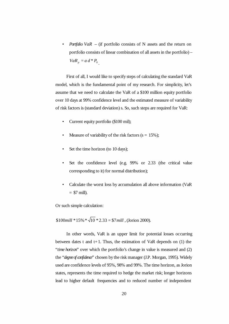
First of all, I would like to specify steps of calculating the standard VaR
model, which is the fundamental point of my research. For simplicity, let’s
assume that we need to calculate the VaR of a $100 million equity portfolio
over 10 days at 99% confidence level and the estimated measure of variability
of risk factors is (standard deviation) s. So, such steps are required for VaR:
• Current equity portfolio ($100 mil);
• Measure of variability of the risk factors (s = 15%);
• Set the time horizon (to 10 days);
• Set the confidence level (e.g. 99% or 2.33 (the critical value
corresponding to it) for normal distribution);
• Calculate the worst loss by accumulation all above information (VaR
= $7 mill).
Or such simple calculation:
millmill 7$33.2*10*%15*100$ = , (Jorion 2000).
In other words, VaR is an upper limit for potential losses occurring
between dates t and t+1. Thus, the estimation of VaR depends on (1) the
“time horizon” over which the portfolio’s change in value is measured and (2)
the “degree of confidence” chosen by the risk manager (J.P. Morgan, 1995). Widely
used are confidence levels of 95%, 98% and 99%. The time horizon, as Jorion
states, represents the time required to hedge the market risk; longer horizons
lead to higher default frequencies and to reduced number of independent

21
observations. By the Basel Committee, internal models approach should
impose 99% confidence level over the 10-business-day time horizon. Also, by
the Basel Committee the optimal time horizon is 10-day, which makes
possible to detect the potential problem and to compare the tradeoff between
this benefit and costs of frequent monitoring. Also, they choose the 99%
confidence level, because it reflects the tradeoff between the desire to stay
safe and the adverse effect of capital requirements on banks returns (Jorion
2000).
3.2 Parametric and Non-Parametric Approaches for VaR
There are really a lot of approaches for calculating VaR, which depend
on the result we are looking for. But each of them also depends on the
methodology applied to the VaR. In my paper I verified two of them: historical
simulations method, as one of non-parametric approaches and delta-normal
valuation (variance-covariance or standard) approach as one of the parametric
methods. There is not one the best method, each of them has its pluses and
minuses (look at the Table 1, Appendix). For historical simulations, the choice
of the returns (deviations) distribution does have a significant consequence
for VaR estimate. It is common to estimate quantiles by assuming normal
distribution. The variance-covariance approach assumes normal distribution
of parameters and does, therefore, not take into account a possible non-
linearity of price-yield relationship. If returns are not normally distributed,
then correlation coefficients are seriously weakened and may give misleading
answers. The normal distribution hypothesis can not be rejected for liquid
markets (stock market), at the same time the illiquid markets (market for
credits and deposits) have often very moderate value changes in a number of
successive days, which leads to a high concentration of values around the
mean. So, I decided to choose these two approaches, because in the case of
our country we would see the difference in prediction by the parametric and
non-parametric methods (look in the literature review). Moreover, the normal
distribution of deviations of interest rates and exchange rates (with high

22
concentration around the mean) supports my choice. On the Figure 1 we can
see the see the normality of distribution deviations of deposits from
Individuals up to one month. There are the similar distributions for every
other type of variable.
Figure 1. Normality of Distribution of Deposits from Individuals Up To
1 Month.
3.3 Method of Historical Simulations
Method of historical simulations is one of non-parametric methods. It
supposes the transferability and validity of historic data for the future. This
means that the market in the future will be stationary, which is assumed in the
case of Ukraine. Historical simulation will never estimate VaR to be larger
than the worst loss observed in the sample. This is the major shortcoming of
this method. The historical data may looks fine, but on the market the history
has no great influence, especially in the liquid markets, where the situation can
change every minute. To use this method, we need to choose the time period
Normality of distribution DF1
-100
0
100
200
300
400
500
600
1 3 5 7 9 11 13 15 17 19 21 23 25
23
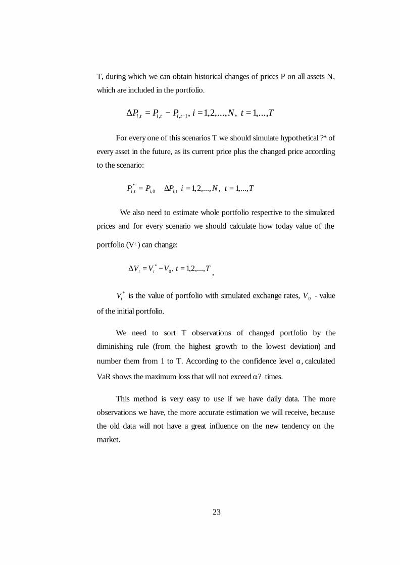
T, during which we can obtain historical changes of prices P on all assets N,
which are included in the portfolio.
TtNiPPP tititi ,...,1,,...,2,1,1,,, ==−=∆ −
For every one of this scenarios T we should simulate hypothetical ?* of
every asset in the future, as its current price plus the changed price according
to the scenario:
TtNiPPP tiiti ,...,1,,...,2,1,0,*, ==∆+=
We also need to estimate whole portfolio respective to the simulated
prices and for every scenario we should calculate how today value of the
portfolio (V t ) can change:
TtVVV tt ,...,2,1,0* =−=∆ ,
*tV is the value of portfolio with simulated exchange rates, 0V - value
of the initial portfolio.
We need to sort T observations of changed portfolio by the
diminishing rule (from the highest growth to the lowest deviation) and
number them from 1 to T. According to the confidence level α, calculated
VaR shows the maximum loss that will not exceed α? times.
This method is very easy to use if we have daily data. The more
observations we have, the more accurate estimation we will receive, because
the old data will not have a great influence on the new tendency on the
market.

24
3.4 Delta-Normal Method (Variance-Covariance Method)
The first and basic assumption for the delta-normal method is that the
portfolio’s yields or the deviations of interest rates are normally distributed.
This assumption is sometimes very convenient, because the portfolios of
normal variables are themselves normally distributed. Jorion (2000) published
the simple technique of how to calculate VaR by var-cov matrix approach. As
this method is appropriate only for linear combinations of risk factor/the
value of instrument, the first step will be to calculate the value of portfolio in
the initial point
)( 00 SVV = , where S is a risk factor.
Taking the derivative of the value in the point, we can define the
sensitivity of portfolio to changes in prices, evaluated in the current
position 0V . This should be called a modified duration ( 0∆ ), so, the value of
potential loss in dV can be computed as:
dSdSSV
dV *00∆=
∂∂
= , where dS involve the potential change
in prices.
In this case (this technique is most appropriate for exchange rate risk
evaluating), the portfolio VaR will be calculated as:
( ) ( )δα ***0 VVaR ∆= , (Jorion 2000).
It should be underlined that with the shorter horizon, Delta-Normal
approximation becomes better, because the quality of approximation depends
on the type of instrument, its maturity, volatility of risk factors and the VaR
horizon (Jorion 2000).
The simulation by the standard local valuation method – Variance-
Covariance should contain such steps:
25
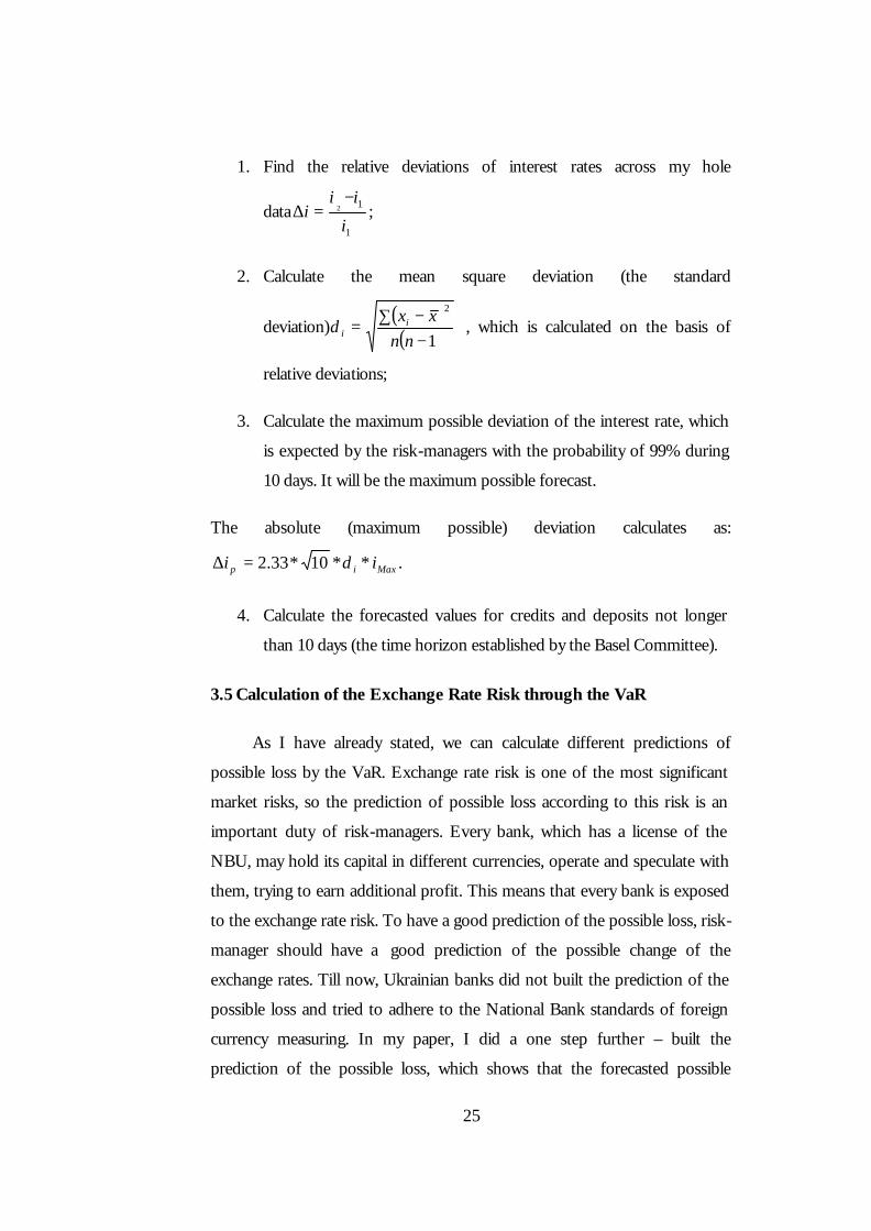
1. Find the relative deviations of interest rates across my hole
data1
12
i
iii
−=∆ ;
2. Calculate the mean square deviation (the standard
deviation) ( )( )1
2
−−∑
=nn
xxiiδ , which is calculated on the basis of
relative deviations;
3. Calculate the maximum possible deviation of the interest rate, which
is expected by the risk-managers with the probability of 99% during
10 days. It will be the maximum possible forecast.
The absolute (maximum possible) deviation calculates as:
Maxip ii **10*33.2 δ=∆ .
4. Calculate the forecasted values for credits and deposits not longer
than 10 days (the time horizon established by the Basel Committee).
3.5 Calculation of the Exchange Rate Risk through the VaR
As I have already stated, we can calculate different predictions of
possible loss by the VaR. Exchange rate risk is one of the most significant
market risks, so the prediction of possible loss according to this risk is an
important duty of risk-managers. Every bank, which has a license of the
NBU, may hold its capital in different currencies, operate and speculate with
them, trying to earn additional profit. This means that every bank is exposed
to the exchange rate risk. To have a good prediction of the possible loss, risk-
manager should have a good prediction of the possible change of the
exchange rates. Till now, Ukrainian banks did not built the prediction of the
possible loss and tried to adhere to the National Bank standards of foreign
currency measuring. In my paper, I did a one step further – built the
prediction of the possible loss, which shows that the forecasted possible

26
maximum should not exceed the calculated amount with 99% of confidence
level. The most important difficulty of this task is in the prediction of the
possible changes in the exchange rate. So, I will simulate the exchange rate
changes on the basis of the NBU (www.finance.com) database. In Bank,
which I analyze, exchange rate risk depends on the portfolio of such
currencies as Hryvna, American Dollar, Euro, Polish Zloty, Canadian Dollar,
Great Britain Pound Sterling and Russian Ruble. The work contains such
steps:
• simulation of possible change the exchange rates (USD/UAH,
EUR/UAH, CAD/UAH, GBP/UAH, RUB/UAH, PLN/UAH).
The simulation for every exchange rate I will do by the 2 methods,
which I described above – historical simulations and variance-
covariance methods;
• estimation of the exchange rate currency position;
• multiplying of the simulated change of the exchange rate on the
estimated currency position by every foreign currency, which is in the
banks’ portfolio;
• 10*33.2** ccPosVaR δ∆= , where
cPos - estimated banks’ position, according to every currency;
c=USD, EUR, CAD, GBP, RUB, PLN;
cδ∆ - simulated change of exchange rate, according to every
currency; c= USD, EUR, CAD, GBP, RUB, PLN ;
2.33 – coefficient, correspondent to the 99% of confidence level;
10 - fixed time horizon.
27
After calculating VaR for every currency separately, we would like to
see the total amount of capital under the exchange rate risk. There are two
possible strategies to do this: we can add together obtained results for every
currency or we can calculate the total matrix of correlation of all exchange
rates. Because of correlation, results should be lower than after simple adding,
because the influence of different factors, which influences one on other in a
single whole, diminishes the influence of separate factors.
3.6 Similar Method to VaR, Based On Historical Simulations and
Delta-Normal Simulations
As I have already mention, traditional VaR is very good for calculating
the possible loss of the bank’s assets where the revaluation of the worth of
the capital is immediate after the factor has changed caused to the asset. For
example, I decided to calculate traditional VaR through Historical simulation
and Delta-Normal simulation for the exchange rates risk. As the exchange
rate changes, so the value of the foreign currency position in the banking
balance sheet changes too. Thus, the classical VaR method is applicable in this
case
But what should we do if there is no immediate revaluation? Such
situation can be shown in my next example with interest rates on the non-
traded banking goods (asset and loans). Really, we can’t adjust the interest rate
according to the today’s market ones on the assets and loans, because we have
already signed agreements about the interest rate on certain duration in the
past. But still we have a risk today; respective to the new market rates the
bank will have the revenue or the loss. That is why the analysis of present
value of bank’s assets and loans should be under the permanent control. Also,
risk-managers should predict possible range of changes the interest rates on
assets and loans in the future. According to this prediction they can also give
some recommendation about what amounts of credits and deposits can be
used and under what interest rates the bank can operate today to hedge the

28
balance of unprofitable and profitable levels. Also, in many foreign studies the
traditional measures of risk of interest rate deviations were focused on the
influence of changes of the interest rate on the net interest margin. But
today’s research provides new assumption that changes of interest rate affect
not only the net interest margin, but also the value of assets and liabilities in
the present time (Buschegen 1998). So, instead of investigating the effect of
interest rate changes on profits, recent methods focus more on the present
value of a bank’s capital.
That is why I am sure that this approach will find its users and strong
support among risk-managers in different financial institutions.
On the basis of analyzed data I did the evaluation of volatility of
interest rates according to historical simulation and variance-covariance
simulation approaches. My data consists of 24 816 observations (almost 3
years of daily observations for UAH, USD and EUR for deposits and credits
up to 1 month, 3 months, 6 months and 12 and more). These are the main
steps that I have done calculating the interest rate risk:
1. For every balance item of assets and loans under the interest rate I
will calculate the present value (PV) as
( )t
jt
i
SPV
+=∞→
1, where
S j – balance value of the ?-item,
i – weighted average interest rate of this item,
t - time.
So, instead of evaluating the influence of interest rate changes on the
profit, we have to focus more on the bank’s present value.
29
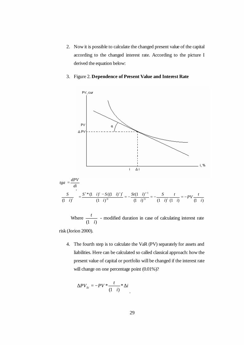
2. Now it is possible to calculate the changed present value of the capital
according to the changed interest rate. According to the picture I
derived the equation below:
3. Figure 2. Dependence of Present Value and Interest Rate
)1()1()1()1()1(
)1())1(()1(*
)1( 2
1
2 it
PVi
ti
SiiSt
iiSiS
iS
didPV
tg
tt
t
t
tt
t +−=
++−=
++
−=+
′+−+′=
′
+
=
−
α
Where )1( i
t+
- modified duration in case of calculating interest rate
risk (Jorion 2000).
4. The fourth step is to calculate the VaR (PV) separately for assets and
liabilities. Here can be calculated so called classical approach: how the
present value of capital or portfolio will be changed if the interest rate
will change on one percentage point (0.01%)?
ii
tPVPV i ∆
+−=∆ ∆ *
)1(*
.
30
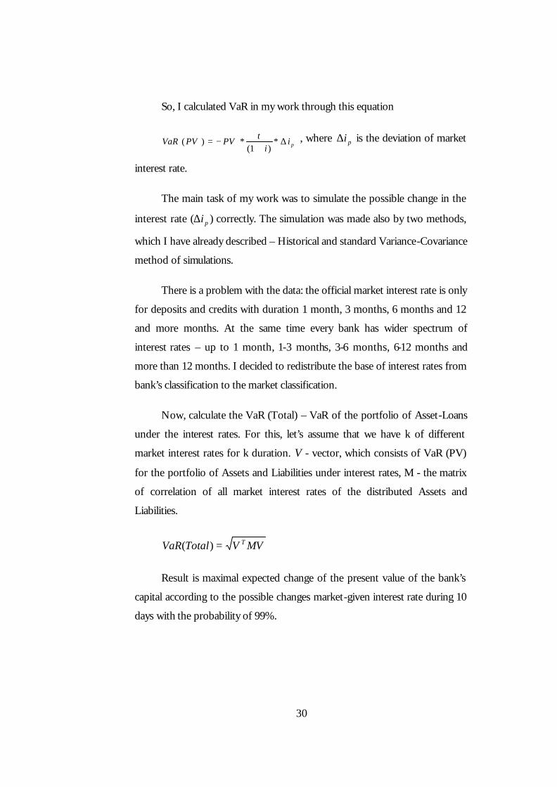
So, I calculated VaR in my work through this equation
pii
tPVPVVaR ∆
+−= *
)1(*)( , where pi∆ is the deviation of market
interest rate.
The main task of my work was to simulate the possible change in the
interest rate ( pi∆ ) correctly. The simulation was made also by two methods,
which I have already described – Historical and standard Variance-Covariance
method of simulations.
There is a problem with the data: the official market interest rate is only
for deposits and credits with duration 1 month, 3 months, 6 months and 12
and more months. At the same time every bank has wider spectrum of
interest rates – up to 1 month, 1-3 months, 3-6 months, 6-12 months and
more than 12 months. I decided to redistribute the base of interest rates from
bank’s classification to the market classification.
Now, calculate the VaR (Total) – VaR of the portfolio of Asset-Loans
under the interest rates. For this, let’s assume that we have k of different
market interest rates for k duration. V - vector, which consists of VaR (PV)
for the portfolio of Assets and Liabilities under interest rates, M - the matrix
of correlation of all market interest rates of the distributed Assets and
Liabilities.
MVVTotalVaR T=)(
Result is maximal expected change of the present value of the bank’s
capital according to the possible changes market-given interest rate during 10
days with the probability of 99%.

31
3.7 Back-Testing
VaR models make sense only in case when they predict risk reasonably
well. According to Jorion, Back-testing is a formal statistical framework that
consists of verifying that actual loss is in line with projected loses. It consists
of the systematic comparison of historical VaR forecasts with the associated
portfolio returns. If the Back-testing shows perfect or acceptable results, we
can conclude that the model we chose is good for forecasting. If not, the
model should be reexamined for the correct assumptions, other parameters or
other model approach. The Back-testing mechanism was the basic point for
the Basel Committee to allow for internal capital requirements in bank use
VaR models. Such controlling measure can help to avoid the situation, when
bank underestimates its risk in order to cooperate on the international level.
Though, system of Back-testing verification should be designed in such a way
as to maximize the probability of detecting banks which would like to
understate their risk (Jorion 2001).
If the model gives a good fit, the number of observations that fall
outside the VaR should correspondent to the chosen confidence level. These
observations that are out of the line are known as the exceptions. If there are
too many exceptions, the model underestimates risk. Here the greatest
problem is hidden, because bank can allocate too little capital to cover the
risk. On the other hand, if the model shows too little exceptions, it can
indicate excess or inefficient capital allocation.
Basel Committee derived its own rules for Back-testing directly from
the failure rate test. There are two possible types of errors: type 1 error means
that the correct model is rejected and the type 2 errors means that the wrong
model is accepted. You can see these results below:

32
Table 1. Types of Errors According to Type of Decision
Model
Decision Correct Incorrect
Accept OK Type 2 error
Reject Type 1 error OK
Also, Basel derived the possible number of exceptions according to
every confidence level. Basel Committee requires from the banks which want
to work on the open market to calculate their VaR with 99% confidence level.
These results are represented below:
Table 2. Basel Committee Requirements to Exceptions
Nonrejection Region for Number of Failures
N Probability
Level p
VaR
Confidence
Level T= 255 days T= 510 days T=1000
days
0.01 99% N<7 1<N<11 4<N<17
0.025 97.5% 2<N<12 6<N<21 15<N<36
0.05 95% 6<N<21 15<N<36 37<N<65
0.075 92.5% 11<N<28 27<N<51 59<N<92
0.1 90% 16<N<36 38<N<65 81<N<120
This table was constructed by Jorion (2000).
33
At the same time Basel constructed 3 categories of results, obtained by
banks. Green zone banks are those that admitted 0-4 exceptions, Yellow zone
– 5-9 exceptions, 10 and more – Red zone. Basel Committee allows to
cooperate on the open market only the banks from the Green zone and
sometimes, according to the market conditions, from the Yellow zone.
The conclusion about the adequacy of chosen model (historical
simulation or variance-covariance simulation) I made on the basis of back-
testing. I compared the predicted deviations of exchange rate and interest rate
with real deviations on the graph, supposed to be lost with the probability
99% with the actual loss. If the back-testing shows acceptable results, the VaR
model is correct. The best forecast with VaR-method is made up to 10 days,
assuming that during this time the situation on the market shouldn’t change
dramatically and the results could be easily adjusted. For the exchange rate
risk the back-testing showed how good the simulated exchange rates fit to the
real. In the case of interest rate risk the back-testing showed how suitable are
simulated numbers of interest rates to the real ones.
We can see Back-test results in numbers, comparing predicted
simulations with real numbers or the obtained results we can see on the
graph. The second way of checking the model is easier and correct, so in my
work I will check the results through the graphs.
If the Back-testing shows good results on the historical numbers, this
means that the future prediction should be good too. Obtained final results
will be used by the risk-managers, as additional method for forecasting the
possible troubles for the bank.

34
C h a p t e r 4
DATA DESCRIPTION
For calculating the exchange rate risk through the VaR method I need
the data of daily exchange rates of the currencies in the bank’s portfolio
(USD/UAH, EUR/UAH, CAD/UAH, GBP/UAH, RUB/UAH,
PLN/UAH or other currencies, which the bank is operating with) and the
corresponding daily currency positions. The classical VaR can easily calculate
the possible loss/gain from this type of risk and I will do it on the basis of
exchange rates data collected on www.finance.com from NBU.
For calculating the amount of capital under the interest rate risk, the
main source I will use is the www.finance.com (Ukraine data). Here, the
obtained data (market interest rates) is calculated in most cases as the
mathematical average of interest rates (by the types), which is collected from
the commercial banks every day. Association of Banks in Ukraine estimates
the market interest rate in such a way too. Also, I will need the bank’s interest
rates for every type of credits and deposits for individuals and corporate
bodies. Also, for simplicity of explanation my results, I did not calculate the
VaR for the real bank’s portfolio, nevertheless this methodology will be valid
in real conditions. I assumed that the portfolio consists of equal sums (UAH
1000, USD 1000 and EUR 1000) of Credits and Deposits under different
interest rates. This will make easier the process of understanding the
methodology, comparing amounts of possible loss that are under different
interest rates of Credits and Deposits, and the explanation of the estimated
results.
I will need the daily data of market interest rate and bank’s interest rate
by credits and loans for individuals and for corporate bodies. So, the data will
include:

35
• Market interest rates on credits for individuals (1 month, 3 months, 6
months, 12 months) and bank’s interest rates on credits for
individuals (up to 1 month, 1-3 months, 3-6 months, 6-12 months
and more than 12 months);
• Market interest rates on credits for corporate bodies (1 month, 3
months, 6 months, 12 months) and bank’s interest rates on credits for
corporate bodies (up to 1 month, 1-3 months, 3-6 months, 6-12
months and more than 12 months);
• Market interest rates on deposits from individual (1 month, 3 months,
6 months, 12 months) and bank’s interest rates on deposits from
individual (up to 1 month, 1-3 months, 3-6 months, 6-12 months and
more than 12 months);
• Market interest rates on deposits from corporate bodies (1 month, 3
months, 6 months, 12 months) and bank’s interest rates on deposits
from corporate bodies (up to 1 month, 1-3 months, 3-6 months, 6-12
months and more than 12 months).
This data is in three types of currency – UAH, USD and EUR and 730
days data is observed.
Whole data set was collected daily from 01.01.2003 to 01.01.2005.
In the summary statistics, which are represented in the Appendix, the
maximal, minimal and mean observations are stated. The total number of
observations is calculated too.

36
C h a p t e r 5
ESTIMATED RESULTS
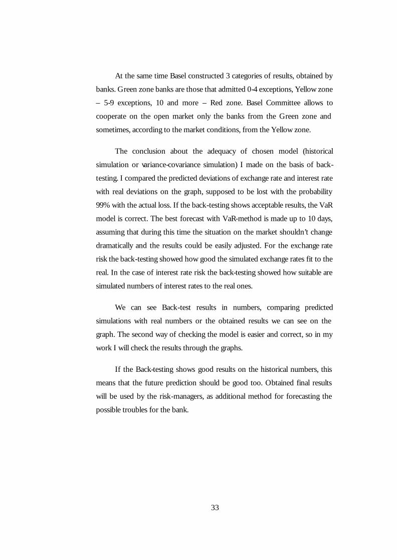
5.1 Back-Testing
Obtained results I presented in the form of graphs and tables. As I
wrote before, to calculate the VaR of interest rate risk I need to have
simulated deviations of the interest rates. The conclusion about accuracy of
simulation procedure is based on the back-testing. So, for example, on the
graphs below you can see the results of provided back-testing for the
simulated deviations of interest rate on credits for individuals up to 1 month
(UAH) and the simulated deviations of interest rate on deposits from
individuals up to 12 months (EUR). Graphs for every other simulated
variable you can see in the Appendixes.
On the first graph you can see three trends: the real trend of interest
rate deviations on credits for individuals up to 1 month (firm line), the trend
of simulated deviations of this interest rate by the historical simulation rule
(darker dotted line) and the trend of simulated deviations of this interest rate
by the variance-covariance (standard) method (lighter dotted line).
As we can see both simulations showed almost the same results, these
both lines are above then the real trend. Why they are above? The simulation
should include all possible worst cases that can happen with the bank.
According to the previous suggestions about present value I can conclude: if
the market interest rate on the credits will rise, the present value of banks’
capital will decline. This is negative situation for the bank. That is why the
simulated changes of interest rate on credits a re above the real trend. Standard
method gave results that are slightly above those given by the historical
simulation method. This means that under the standard method of simulation
37
the bank is more assured from negative events then under the historical
simulation method. In this case banks’ risk-managers should be more oriented
on the standard simulation method, which gives more secure results. Of
course, if bank are ready to risk, it can choose historical simulation method, to
have higher revenue. Looking on these trends, we can see two interceptions
with the real data deviations. These interceptions should be called exceptions.
According to the Basel Committee requirements, for the 99% confidence
level prediction and 510 days is permitted to have up to 11 such exceptions
(Table 2). So, my forecast gives reliable results.
Figure 3. Back-testing: Credits for Individuals Up To 1 Month
22,00
22,20
22,40
22,60
22,80
23,00
23,20
23,40
23,60
23,80
24,00
01.01.2004 01.02.2004 01.03.2004 01.04.2004 01.05.2004 01.06.2004 01.07.2004 01.08.2004 01.09.2004 01.10.2004 01.11.2004 01.12.2004
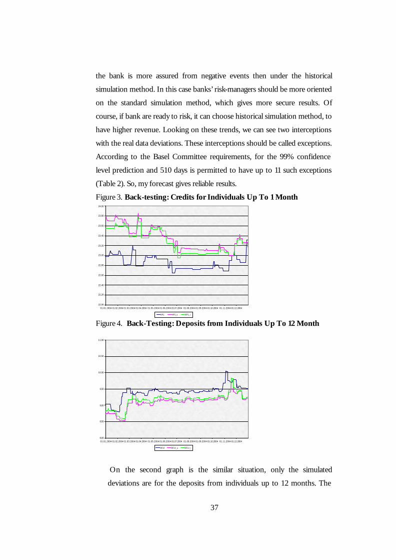
KF1 KF1_s KF1_i Figure 4. Back-Testing: Deposits from Individuals Up To 12 Month
8,00
8,50
9,00
9,50
10,00
10,50
11,00
01.01.2004 01.02.2004 01.03.2004 01.04.2004 01.05.2004 01.06.2004 01.07.2004 01.08.2004 01.09.2004 01.10.2004 01.11.2004 01.12.2004
DF12 DF12_s DF12_i
On the second graph is the similar situation, only the simulated
deviations are for the deposits from individuals up to 12 months. The
38
simulated trends are below the real data deviations. Such situation is
because for every bank the worse situation is if the market deposits
interest rate decreases. This means that the bank’s capital present value
falls and bank will have less profit. Simulated trends on this graph show
almost the same predictions too. Again the variance-covariance method
gives more secure results of the simulated deviations. In this case bank
should be oriented on the standard method to be surer in the capital
safety. Moreover, the standard simulation method has no exceptions and
the historical simulation method has one exception.
Similar results of back-testing we can observe for every other variable.
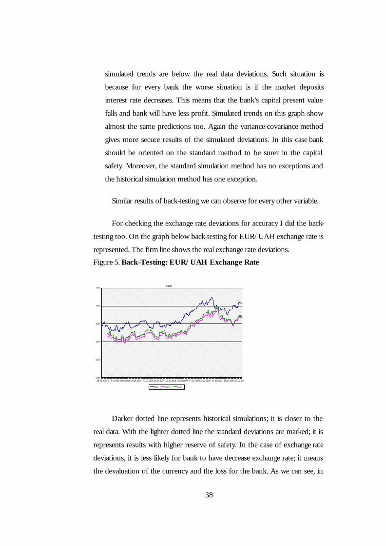
For checking the exchange rate deviations for accuracy I did the back-
testing too. On the graph below back-testing for EUR/UAH exchange rate is
represented. The firm line shows the real exchange rate deviations.
Figure 5. Back-Testing: EUR/UAH Exchange Rate
EUR
5,00
5,50
6,00
6,50
7,00
7,50
29.03.2004 27.04.2004 28.05.2004 29.06.2004 27.07.2004 25.08.2004 22.09.2004 20.10.2004 17.11.2004 15.12.2004 17.01.2005 14.02.2005 15.03.2005
EUR EUR_S EUR_i
Darker dotted line represents historical simulations; it is closer to the
real data. With the lighter dotted line the standard deviations are marked; it is
represents results with higher reserve of safety. In the case of exchange rate
deviations, it is less likely for bank to have decrease exchange rate; it means
the devaluation of the currency and the loss for the bank. As we can see, in

39
the case of Euro exchange rate deviation simulations the standard method
showed only one exception, which means that this is a good prediction
according to the Basel Committee requirements.
5.2 Value-at-Risk Results, Interest Rate Deviations
Lets look on the estimated results of possible loss of present value the
banks’ capital resulting from the deviations of the interest rate. I will explain
the results I have received on the example of the calculated VaR for the
credits to firms in UAH. The table with these results you can see below.
The first line contains real data – real market interest rate on the
31.12.04 for different duration. Delta-rate (variance-covariance and historical
simulations) means the simulated deviations of the market interest rate by the
chosen methods – standard and historical simulations.
The next section contains data from the “Kredyt-Bank (Ukraine)”
(interest rates and durations). But I decided to take portfolios for every type
of credits and deposits in the same amounts for the simplicity of explanation.
So, the sum of credits and deposits will be unreal, equal for different deposits
and loans. Interest rates that are represented in the line below are the real
bank’ interest rates on credits of different duration. Duration means the
number of days in a certain time period. The next line contains the calculated
future value of every portfolio under the certain interest rate and the
corresponding number of days.
As we can see, the market data includes four columns for 1 month, 3
months, 6 months and 12 months. At the same time, the bank’s data is five
time-periods. To solve the problem of this disparity, I recalculated the market
data (4-segment data) according to the bank’s data (5-segment data).
By the same principle I recalculated the obtained deviations of the
interest rate to have five time-periods. The next line, as we can see, is the

40
calculated present value of the portfolio. I will need this index to calculate the
Value-at-Risk. So, the next line is my first result – calculated VaR by the
formula described in the methodology and according to my data. VaR 1 by
the segments contains calculated results by the variance-covariance simulation
method for time-segments, acceptable to bank. VaR 2 means calculated VaR
by the historical simulation method. VaR 1 and VaR 2 by the duration include
same results recalculated to the market standards. In order to see the possible
loss of present value the portfolio of credits to firms in UAH with probability
99% for 10 days time horizon, I constrained the matrix from vectors of
correlation of the calculated VaRs. Finally, I received VaR 1 (by the variance-
covariance method of simulation) that is equal 5.49 and VaR 2 (by the
historical method of simulation) that is equal 4.75 from total amount of
capital 5000 UAH. This loose is equal 0.11% (0.095%) of total sum.
According to the back-testing, the first method should give us more secure
results, then the second. Our forecast became true, because VaR 1 is larger
then the VaR 2.
Table. 3 VaR for the Credits to Firms, UAH
Market Data 1M 3M 6M 12M Market Interest Rate
(Last)_31.12.04 22,45% 23,00% 23,73% 24,23% Delta -Rate (Var-Cov. sim) 0,36% 0,32% 0,23% 0,22%
Delta -Rate (Hist. sim) 0,30% 0,29% 0,20% 0,19%
Credits <1m 1-3m 3-6m 6-12m >12m Sum Input Data
Sum 1 000,00 1 000,00 1 000,00 1 000,00 1 000,00 5 000,00 Interest Rate 21,23% 21,33% 20,97% 20,78% 19,78% 19,18%
Durarion 24 40 150 300 600 FV 1 012,74 1 023,38 1 086,18 1 170,79 1 325,15 5 618,24
Waighted Average Market Interest Rate 22,45% 22,52% 23,46% 24,05% 24,23%
Waighted Average Delta-Rate (Var-Cov) 0,36% 0,35% 0,s26% 0,22% 0,22%
Waighted Average Delta-Rate (Hist.sim) 0,30% 0,30% 0,24% 0,19% 0,19%
PV 999,34 1 000,85 996,06 980,73 927,62 4 904,60 PV/S 0,9993 1,0008 0,9961 0,9807 0,9276 0,9809
VAR 1 (PV) by the Diapasons -0,19 -0,32 -0,87 -1,45 -2,68 -5,50 VAR 2 (PV) by the Diapasons -0,16 -0,27 -0,78 -1,25 -2,30 -4,76

41
VAR 1 (PV) by the Durations -0,46 -0,36 -1,07 -3,60 -5,50 VAR 2 (PV) by the Durations -0,40 -0,32 -0,94 -3,10 -4,76
-0,46 -0,36 -1,07 -3,60 1,0000 0,9787 0,9699 0,9632 -0,46 Matrix of Correlation Market Interest Rates 0,9787 1,0000 0,9969 0,9922 -0,36 0,9699 0,9969 1,0000 0,9978 -1,07 0,9632 0,9922 0,9978 1,0000 -3,60 VAR 1 (Credit Portfolio) 5,49 -0,40 -0,32 -0,94 -3,10 1,0000 0,9787 0,9699 0,9632 -0,40 Matrix of Correlation Market Interest Rates 0,9787 1,0000 0,9969 0,9922 -0,32 0,9699 0,9969 1,0000 0,9978 -0,94 0,9632 0,9922 0,9978 1,0000 -3,10 VAR 2 (Credit Portfolio) 4,75
What these results mean? According to the Value-at-Risk definition, assumed
portfolio, real rates and their simulations: “Kredyt-Bank (Ukraine)” is exposed
to the loss of 0.11% (0.095%) of total portfolio with the probability 99%
during 10 days time horizon if the market interest rates on credits to firms will
deviates as the standard method (historical simulation method) predict.
The similar explanation is acceptable for every table with estimated
results in Appendixes.
The last step in calculating of the possible loss according to the interest
rate deviations was to construct the huge matrix of correlation of all VaRs
calculated for every credit and deposit in every currency. The matrix gave
such results: VaR by the standard method shows the possible loss UAH
168.23 and the VaR by the historical method shows the possible loss UAH
155.18, which means that the bank with assumed portfolio is exposed to loose
0.28% (0.25%) of total (5000 UAH, 500 EUR and 5000 USD) capital that is
under the interest rate risk. This is not the great loose, but nevertheless we
should be secure of this risk. Taking the real “Kredyt-Bank (Ukraine)”
portfolio, which is equal to 1 250 mln UAH, the possible loss of capital
42
according to interest rate is equal 3.36 mln UAH by the standard method and
3 mln by historical simulations method.
5.3 Value-at-Risk, Exchange Rates Deviations
In Appendix we can see the table with calculated possible loss
according to the risk of the exchange rate deviations on the example of the
“Kredyt-Bank (Ukraine)”. Such risk is possible if bank has open position in
currency with possible risk of volatility. I again assumed that the open
position in every currency is equal to the same sum 1000. This is impossible
situation in reality, but such assumption makes easier the explanation of the
VaR. The next two lines (sigma standard and sigma historical) contain
forecasted deviations of the exchange rates according to the standard method
and historical simulation respectively.
According to the formula from the methodology I calculated VaR for
every currency by these two methods. To see the total picture of possible loss
of capital according to the deviations of the exchange rates I constructed the
matrix of correlation of VaRs for every currency. These results also confirmed
the back-testing forecast that variance-covariance method gives more secure
results. So, VaR by the standard method is equal UAH 957.42 and the VaR by
the historical simulation method is equal 831.72. We can understand these
results as bank with such exchange rates and such portfolios is exposed to the
loss 3.19% (2.77%) of total (1000 USD, 1000 EUR, 1000 PLN, 1000 CAD,
1000 GBP, 1000 RUB) capital from combined portfolio with the probability
99% during 10 days time-horizon according to the predicted change of the
exchange rates by the standard method (historical simulation method).
43
C h a p t e r 6
IMPLICATIONS
In this paper I have evaluated interest rate and exchange rate risks
through the recommended methodology by Basel Committee II – VaR.
Which results I got and how can I extrapolate them to give a piece of
good advice to the Asset and Loan Administration? First of all, let’s look to
the fina l results. VaR showed me that the “Kredyt-Bank (Ukraine)” is
exposed to loose 3.6 mln UAH by var-cov method (3 mln UAH by historical
method) according to the real interest rates, bank’s rates and portfolio.
Calculated VaR shows the waste capital because of volatility of interest rates.
These both sums show the cumulated loss of all interest rates deviations.
Hence, we can say that the interest rate risk in “Kredyt-Bank (Ukraine)” is
equal to 3.6 mln UAH (3 mln UAH) with probability 99% for 10 days time
horizon according to asset-loan portfolio.
Cumulated exchange rate risk is equal to the total VaR for all currencies
from the assumed portfolio. In the case of “Kredyt-Bank (Ukraine)” I could
not calculate total VaR because the information about open positions (long
and short) are closed information. But the final proportions of possible loss
will be the same: total amount of capital under the risk is equal to 3.19% of
total portfolio by standard method (2.77% by historical simulation method).
Such results I got after calculating VaR for the portfolio of foreign currencies
(1000 every currency) and real exchange rates.
44
Besides these results I have calculated VaR for every interest rate for
loans and deposits, individuals and firms; also I have calculated VaR fore
every currency.
How can I manage these results?
National Bank in Ukraine determines different quotes to the
commercial banks. Commercial banks should cooperate within these quotes;
otherwise they will have different penalties or could be announced as
bankrupts.
One of these quotes is the ratio of Capital Adequacy. It is calculated as
Required Capital divided on the Bank’s Assets, adjusted to the risk on every
loan. National Bank of Ukraine decided measure this index not less than 10%
(according to the Basel Committee, for developed world banks this ratio
should be not less than 8%). We have this ratio slight higher, because in
calculating loans adjusted on risk only credit risk should be included by the
Ukrainian legislation. By the Basel Committee requirements, all risks should
be included into this quota. Hence, constructing the internal model of risk-
measurement the manager can include calculated amount of interest rate risk
and exchange rate risk in calculating Capital Adequacy. This index will
become lover, approaching our banks to the Basel requirements. Moreover,
now “Kredyt-Bank (Ukraine)” will be insured the market risk and at the same
time it will be more compatible to other banks, having better index of Capital
Adequacy. So, managers’ task should be to keep this index so close to 10%, as
possible, but not less. Bank in that case will have the possibility to earn more
and to have under the control interest rate risk and exchange rate risk.
Now, how managers can manage the amount of risks? According to
obtained results by VaR we can see the picture, what is the most risky and
what is less risky. My results showed that the biggest amount of capital under
the risk is in the sector of Deposit from Individuals in EUR, where VaR of
5000 EUR portfolio is equal to 9.87 EUR (0.197%) by the standard method

45
and 9.34 (0.19%) by the var-cov method. Minimal amount of capital can be
lost according to the interest rate risk in the sector of Credits to Firms in
UAH. – 5.49 UAH (0.11%) by the standard method and 4.75 UAH (0.095) by
the historical simulation method of 5000 UAH portfolio. Looking on results
of the exchange rate risk, you can see the smallest possible loss in 1000 RUB
– 2.4 RUB (0.04% of total portfolio) by the standard method (2.91 RUB (0.05
%) by the historical simulation method) and the maximal possible loss in 1000
GBP – 423.58 GBP (7.05% of total portfolio) by the standard method
(368.54 GBP (6.14%) by the historical simulation method).
Hence, looking on these results, risk-manager can advice to the Asset
and Loan Administration to reduce the amount of Deposits from Individuals
in EUR (or to hold them under very strong control) and increase amount of
Credits to Firms in UAH. Also, the bank should increase amounts contracts
in RUB and decrease amount of contracts in GBP. Such steps will lead to
diminished amount of total VaR and to correct and rational ratio of Capital
Adequacy. In the nearest future this internal bank’s policy can make easier
transition to the Basel Committee (and developed world) standards of risk-
measurement!

46
C h a p t e r 7
CONCLUSION
Today Ukraine stands on the new level of its development. The
possibility of cooperation on the open financial market, as the full-right
partner opens before the native commercial banks. But to be strong
competitors and loyal partners they should reconsider some basic standards.
One of these standards is risk-management. Because of high effectiveness of
VaR methodology, it is widely used in the world. It helps to see the risky of
the business process, diversify the portfolio of assets. Also it helps to attract
big investors.
VaR modeling for the assessment of interest rate risk and exchange rate
risk has an advantage of comparability of sensitivity of assets or portfolio on
different risk factors. Also, it can be calculated the total amount of capital
under the risk.
However, the precision of VaR prediction depends on the underlying
conditions. For analysis the empiric data revealed that traditional VaR
calculating is not always the best method for calculating possible loss. For
example, for calculating amount of capital under the interest rate risk in bank,
the better solution will be to calculate VaR through the PV.
The performance comparison of historical simulations and var-cov-
simulation methods for VaR prediction for both risks (interest rate risk and
exchange rate risk) are suitable for implementation on such market, as
Ukraine. However, here is a great shortcoming; still our market interest rate is
not adjusted with the market processes. That is why the correlation between
47
the market interest rate and real bank interest rate can be very weak.
However, for developed markets VaR remains a very useful too; for
evaluating, controlling and management all kinds of risk.
Currently Ukrainian market should find VaR very useful for evaluation
the risk of bank’s activity. Ukrainian banks are ready to apply Basel’s required
methodology in their risk management. New approach will turn over the
traditional view on risk management. VaR will make our financial institutions
more compatible on the open financial market, will raise clients’ trust and will
gain world’s confidence. So, VaR-measurement should be a very important
point in the today’s policy of changes.
Nevertheless, VaR and all methodologies for its calculating are not the
“panacea” for bank’s health. Everybody has a right to choose something very
individual or new if it will bring him needed information for good
management.
48
BIBLIOGRAPHY
Aragones, Jose. R., Carlos Blanco, Kevin Dovd. “Learning Curve Extreme Value VaR”, March 6 2001.
Bams Dennis, Jacco L. Wielhouwer.
“Empirical Issues in Value-at-Risk”, December 2000.
Basel Committee on Banking
Supervision. “Principles for the Management and Supervision of Interest Rate Risk”. July 2004.
Butler Comas. “Hidings of Value-At-
Risk”. Practical Aid for Using VaR 2001.
Dowd B. Kevin. “The Extreme Value
Approach to VaR – an Introduction, Part 4”, 1995.
Jorion Phillipe. “Value-at-Risk”,
McGraw-Hill, 1997. Jorion Phillipe. “Value-at-Risk”,
McGraw-Hill, 2000. Jorion Phillipe. “Value-at-Risk”,
McGraw-Hill, 2001. Ho Lan-Chih, Peter Burridge, John
Cadle, Michael Theobald. “Value-at-Risk: Applying the Extreme Value Approach to Asian Markets in the Recent Financial Turmoil”. Pacific-Basin Finance Journal 8. 2000, 249–275.
Holton Glyn A. “History of Value-at-
Risk”, July 25, 2002.
Longin Francois M. “The Asymptotic Distribution of Extreme Stock Market Returns”. The Journal of Business, Vol.69,N3(Jul.,1996),383-408.
Lucas Andre. “Evaluating the Basel
Guidelines for Basketing Banks’Internal Risk Management Models”. Journal of Money, Credit and Banking, Vol. 33, N. 3 (Aug.2001).
Manfredo Mark, Raymond M.
Leuthold. “Agricultural Applications of Value-at-Risk Analysis: A Perspective”, 1997.
Marcowitz, Harry M. “Portfolio
Selection”, Journal of Finance, 7(1), 77-91, (1952).
Morgan J.P. “Introduction to
RiskMetrics”, New York, 1995. Rogov M. A. “Risk-Management”,
Finance and Statistic, 2001. Roy, Arthur D. “Safety First and the
Holding of Assets”, Econometrics, 20 (3), 431-449, (1952).
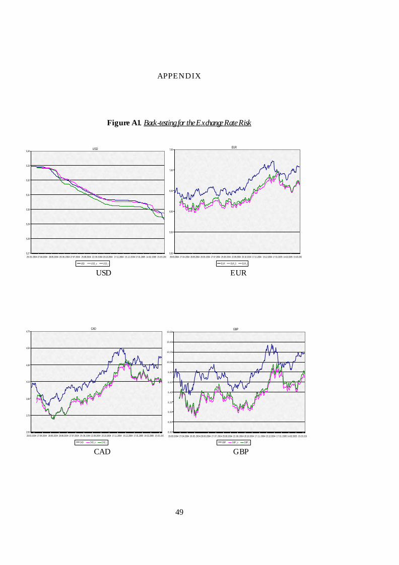
49
APPENDIX
Figure A1. Back-testing for the Exchange Rate Risk
USD
5,27
5,28
5,29
5,30
5,31
5,32
5,33
5,34
29.03.2004 27.04.2004 28.05.2004 29.06.2004 27.07.2004 25.08.2004 22.09.2004 20.10.2004 17.11.2004 15.12.2004 17.01.2005 14.02.2005 15.03.2005
USD USD_s USD_i
EUR
5,00
5,50
6,00
6,50
7,00
7,50
29.03.2004 27.04.2004 28.05.2004 29.06.2004 27.07.2004 25.08.2004 22.09.2004 20.10.2004 17.11.2004 15.12.2004 17.01.2005 14.02.2005 15.03.2005
EUR EUR_S EUR_i USD EUR
CAD
3,50
3,70
3,90
4,10
4,30
4,50
4,70
29.03.2004 27.04.2004 28.05.2004 29.06.2004 27.07.2004 25.08.2004 22.09.2004 20.10.2004 17.11.2004 15.12.2004 17.01.2005 14.02.2005 15.03.2005
CAD CAD_s CAD_i
GBP
8,60
8,80
9,00
9,20
9,40
9,60
9,80
10,00
10,20
10,40
10,60
29.03.2004 27.04.2004 28.05.2004 29.06.2004 27.07.2004 25.08.2004 22.09.2004 20.10.2004 17.11.2004 15.12.2004 17.01.2005 14.02.2005 15.03.2005
GBP GBP_s GBP_i CAD GBP
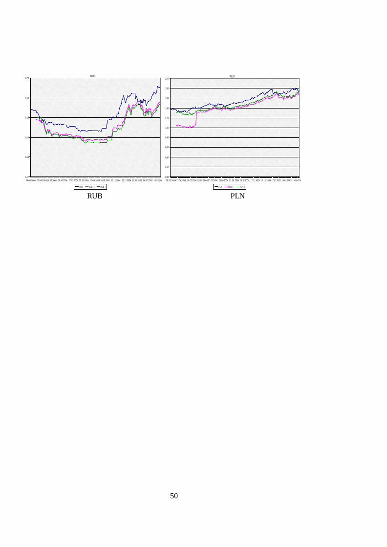
50
RUB
0,17
0,18
0,18
0,19
0,19
0,20
29.03.2004 27.04.2004 28.05.2004 29.06.2004 27.07.2004 25.08.2004 22.09.2004 20.10.2004 17.11.2004 15.12.2004 17.01.2005 14.02.2005 15.03.2005
RUB RUB_s RUB_i
PLN
0,00
0,20
0,40
0,60
0,80
1,00
1,20
1,40
1,60
1,80
2,00
29.03.2004 27.04.2004 28.05.2004 29.06.2004 27.07.2004 25.08.2004 22.09.2004 20.10.2004 17.11.2004 15.12.2004 17.01.2005 14.02.2005 15.03.2005
PLN PLN_s PLN_i RUB PLN
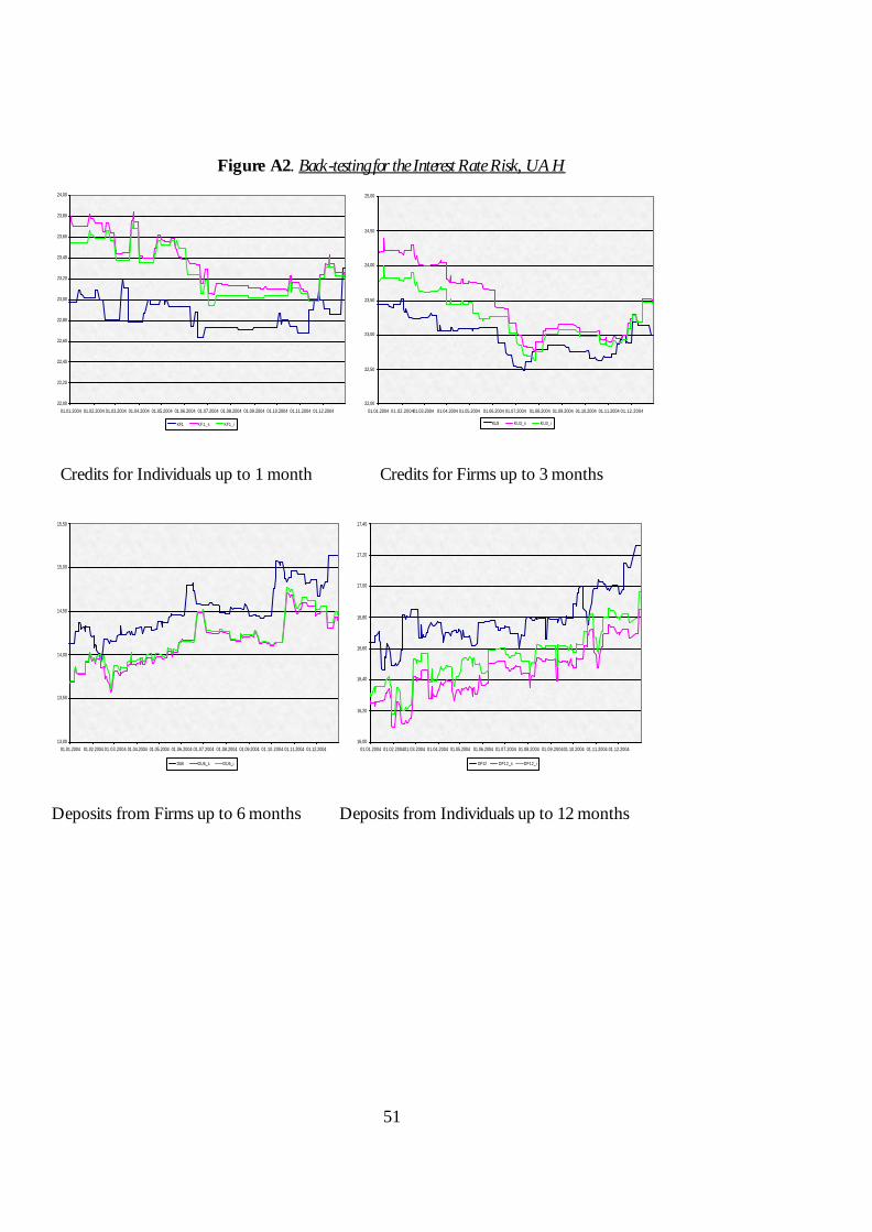
51
Figure A2. Back-testing for the Interest Rate Risk, UAH
22,00
22,20
22,40
22,60
22,80
23,00
23,20
23,40
23,60
23,80
24,00
01.01.2004 01.02.2004 01.03.2004 01.04.2004 01.05.2004 01.06.2004 01.07.2004 01.08.2004 01.09.2004 01.10.2004 01.11.2004 01.12.2004
KF1 KF1_s KF1_i
22,00
22,50
23,00
23,50
24,00
24,50
25,00
01.01.2004 01.02.200401.03.2004 01.04.2004 01.05.2004 01.06.2004 01.07.2004 01.08.2004 01.09.2004 01.10.2004 01.11.2004 01.12.2004
KU3 KU3_s KU3_i
Credits for Individuals up to 1 month Credits for Firms up to 3 months
13,00
13,50
14,00
14,50
15,00
15,50
01.01.2004 01.02.2004 01.03.2004 01.04.2004 01.05.2004 01.06.2004 01.07.2004 01.08.2004 01.09.2004 01.10.2004 01.11.2004 01.12.2004
DU6 DU6_s DU6_i
16,00
16,20
16,40
16,60
16,80
17,00
17,20
17,40
01.01.2004 01.02.200401.03.2004 01.04.2004 01.05.2004 01.06.2004 01.07.2004 01.08.2004 01.09.200401.10.2004 01.11.2004 01.12.2004
DF12 DF12_s DF12_i
Deposits from Firms up to 6 months Deposits from Individuals up to 12 months
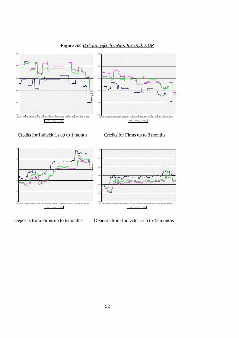
52
Figure A3. Back-testing for the Interest Rate Risk EUR
14,50
15,00
15,50
16,00
16,50
17,00
01.01.2004 01.02.2004 01.03.2004 01.04.2004 01.05.2004 01.06.2004 01.07.2004 01.08.2004 01.09.2004 01.10.2004 01.11.2004 01.12.2004
KF1 KF1_s KF1_i
14,50
15,00
15,50
16,00
16,50
17,00
01.01.2004 01.02.2004 01.03.2004 01.04.200401.05.2004 01.06.2004 01.07.2004 01.08.2004 01.09.2004 01.10.2004 01.11.2004 01.12.2004
KU3 KU3_s KU3_i
Credits for Individuals up to 1 month Credits for Firms up to 3 months
6,00
6,50
7,00
7,50
8,00
8,50
01.01.2004 01.02.2004 01.03.2004 01.04.2004 01.05.2004 01.06.2004 01.07.2004 01.08.2004 01.09.2004 01.10.2004 01.11.2004 01.12.2004
DU6 DU6_s DU6_i
8,00
8,50
9,00
9,50
10,00
10,50
11,00
01.01.2004 01.02.200401.03.2004 01.04.2004 01.05.2004 01.06.2004 01.07.2004 01.08.2004 01.09.200401.10.2004 01.11.2004 01.12.2004
DF12 DF12_s DF12_i
Deposits from Firms up to 6 months Deposits from Individuals up to 12 months

53
Figure A4. Back-testing for the Interest Rate Risk, USD
15,00
15,20
15,40
15,60
15,80
16,00
16,20
16,40
16,60
16,80
17,00
01.01.2004 01.02.2004 01.03.2004 01.04.2004 01.05.2004 01.06.200401.07.2004 01.08.2004 01.09.2004 01.10.2004 01.11.2004 01.12.2004
KF1 KF1_s KF1_i
15,00
15,20
15,40
15,60
15,80
16,00
16,20
16,40
16,60
16,80
17,00
01.01.2004 01.02.2004 01.03.2004 01.04.2004 01.05.2004 01.06.2004 01.07.2004 01.08.2004 01.09.2004 01.10.2004 01.11.2004 01.12.2004
KU3 KU3_s KU3_i
Credits for Individuals up to 1 month Credits for Firms up to 3 months
7,00
7,20
7,40
7,60
7,80
8,00
8,20
8,40
01.01.2004 01.02.2004 01.03.2004 01.04.2004 01.05.2004 01.06.2004 01.07.2004 01.08.2004 01.09.200401.10.2004 01.11.2004 01.12.2004
DU6 DU6_s DU6_i
9,00
9,20
9,40
9,60
9,80
10,00
10,20
10,40
10,60
10,80
11,00
01.01.2004 01.02.200401.03.2004 01.04.2004 01.05.2004 01.06.2004 01.07.2004 01.08.2004 01.09.2004 01.10.2004 01.11.2004 01.12.2004
DF12 DF12_s DF12_i
Deposits from Firms up to 6 months Deposits from Individuals up to 12 Months
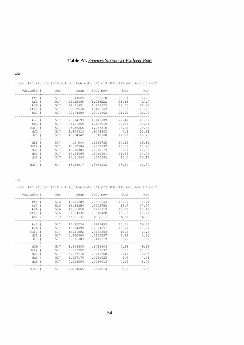
54
Table A1. Summary Statistics for Exchange Rates
UAH
. sum kf1 kf3 kf6 kf12 ku1 ku3 ku6 ku12 df1 df3 df6 df12 du1 du3 du6 du12 Variable | Obs Mean Std. Dev. Min Max -------------+-------------------------------------------------------- kf1 | 517 23.44524 .8581318 22.64 26.8 kf3 | 517 24.45468 1.068522 23.13 27.7 kf6 | 517 24.95451 1.132623 23.55 28.67 kf12 | 517 25.2548 1.476562 23.31 29.76 ku1 | 517 22.74509 .9091362 21.92 26.09 -------------+-------------------------------------------------------- ku3 | 517 23.74193 1.146089 22.47 27.52 ku6 | 517 24.61569 1.183019 23.38 28.31 ku12 | 517 25.36265 1.257515 23.98 29.33 df1 | 517 8.976015 .9458305 7.6 11.38 df3 | 517 13.34342 .618668 12.23 15.26 -------------+-------------------------------------------------------- df6 | 517 15.044 .3286725 14.33 16.16 df12 | 517 16.63584 .2302937 16.15 17.26 du1 | 517 10.10903 .7940119 8.69 12.36 du3 | 517 12.64466 .5012301 11.63 14.02 du6 | 517 14.21269 .3743836 13.5 15.14 -------------+-------------------------------------------------------- du12 | 517 15.84017 .3654222 15.31 16.89 USD . sum kf1 kf3 kf6 kf12 ku1 ku3 ku6 ku12 df1 df3 df6 df12 du1 du3 du6 du12 Variable | Obs Mean Std. Dev. Min Max -------------+-------------------------------------------------------- kf1 | 516 16.03209 .3565943 15.53 17.4 kf3 | 516 16.39254 .5402753 15.7 17.97 kf6 | 516 16.61058 .6773313 16.02 18.47 kf12 | 516 16.4932 .8610428 15.65 18.71 ku1 | 517 15.52346 .2733999 15.11 16.26 -------------+-------------------------------------------------------- ku3 | 517 15.83224 .2445459 15.51 16.83 ku6 | 517 16.14099 .2854351 15.79 17.21 ku12 | 517 16.31002 .3176553 15.9 17.5 df1 | 517 4.490503 .5305337 3.86 5.91 df3 | 517 6.816383 .7449319 5.75 8.62 -------------+-------------------------------------------------------- df6 | 517 8.316808 .6466308 7.28 9.32 df12 | 517 9.653752 .6082637 8.66 10.59 du1 | 517 5.077718 .3712568 4.47 6.35 du3 | 517 6.527176 .4531023 5.9 7.48 du6 | 517 7.614894 .4089013 7.06 8.45 -------------+-------------------------------------------------------- du12 | 517 8.814565 .528014 8.1 9.65

55
Kf (1, 3, 6, 12) – credits to Individuals (up to 1, 3, 6, 12 months)
Ku (1, 3, 6, 12) – credits to Firms (up to 1, 3, 6, 12 months)
Df (1, 3, 6, 12) – deposits from Individuals (up to 1, 3, 6, 12 months)
Du (1, 3, 6, 12) – deposits from Firms (up to 1, 3, 6, 12 months)

56
Table A2. Assessment of Parametric and Non-parametric VaR Models
Model of
risk
assessment
Advantages Disadvantages
Historical
simulation
• Applicable for all types
of price risks;
• Permits non-normal
distribution;
• Is good for non-linear
instruments;
• Integration of many
risk types, low
possibility of model
risk;
• Recommended by the
Basel Committee.
• Transformation of
the historical data
into the future;
• No information
between correlation
with risk factors;
• The same price
trajectory for every
commodity.
Monte-
Carlo
simulation
• Statistically “clean”
method;
• The most flexible of all
estimation techniques.
• Requires a lot of
calculations or
specific computer
software;
• Assumption about
the normality of
distribution.
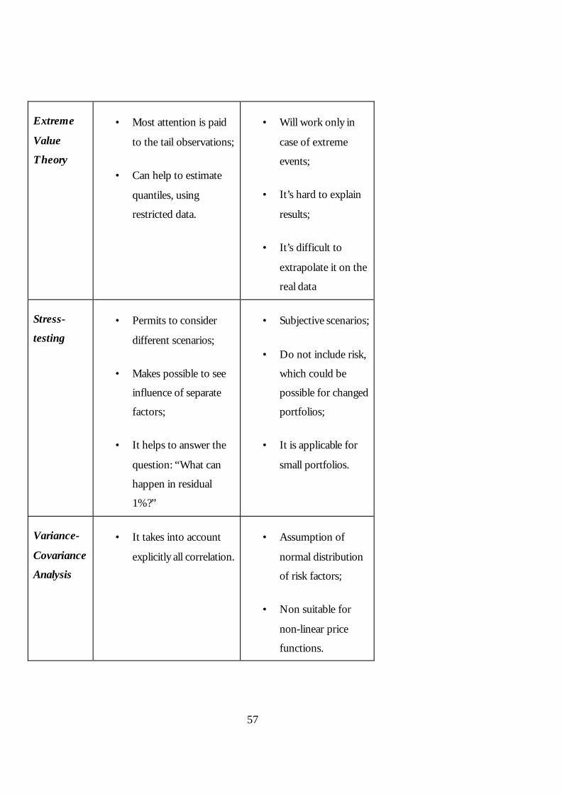
57
Extreme
Value
Theory
• Most attention is paid
to the tail observations;
• Can help to estimate
quantiles, using
restricted data.
• Will work only in
case of extreme
events;
• It’s hard to explain
results;
• It’s difficult to
extrapolate it on the
real data
Stress-
testing • Permits to consider
different scenarios;
• Makes possible to see
influence of separate
factors;
• It helps to answer the
question: “What can
happen in residual
1%?”
• Subjective scenarios;
• Do not include risk,
which could be
possible for changed
portfolios;
• It is applicable for
small portfolios.
Variance-
Covariance
Analysis
• It takes into account
explicitly all correlation.
• Assumption of
normal distribution
of risk factors;
• Non suitable for
non-linear price
functions.
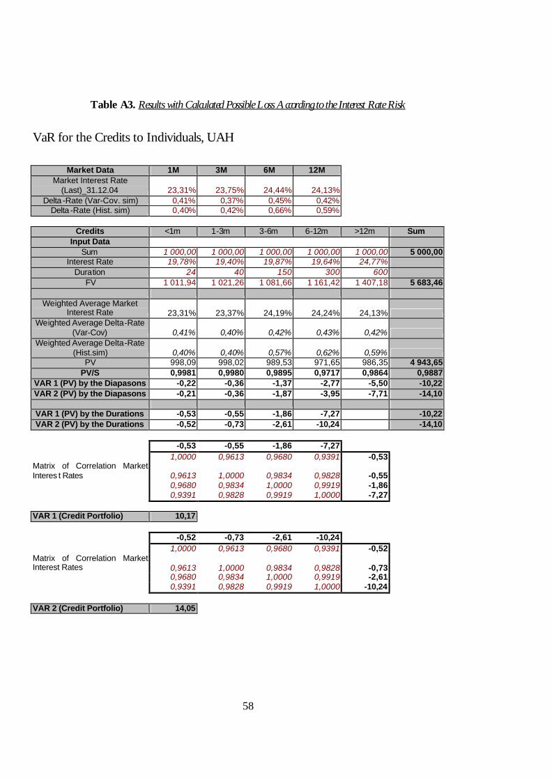
58
Table A3. Results with Calculated Possible Loss According to the Interest Rate Risk
VaR for the Credits to Individuals, UAH
Market Data 1M 3M 6M 12M
Market Interest Rate (Last)_31.12.04 23,31% 23,75% 24,44% 24,13%
Delta -Rate (Var-Cov. sim) 0,41% 0,37% 0,45% 0,42% Delta -Rate (Hist. sim) 0,40% 0,42% 0,66% 0,59%
Credits <1m 1-3m 3-6m 6-12m >12m Sum
Input Data Sum 1 000,00 1 000,00 1 000,00 1 000,00 1 000,00 5 000,00
Interest Rate 19,78% 19,40% 19,87% 19,64% 24,77% Duration 24 40 150 300 600
FV 1 011,94 1 021,26 1 081,66 1 161,42 1 407,18 5 683,46
Weighted Average Market Interest Rate 23,31% 23,37% 24,19% 24,24% 24,13%
Weighted Average Delta-Rate (Var-Cov) 0,41% 0,40% 0,42% 0,43% 0,42%
Weighted Average Delta-Rate (Hist.sim) 0,40% 0,40% 0,57% 0,62% 0,59%
PV 998,09 998,02 989,53 971,65 986,35 4 943,65 PV/S 0,9981 0,9980 0,9895 0,9717 0,9864 0,9887
VAR 1 (PV) by the Diapasons -0,22 -0,36 -1,37 -2,77 -5,50 -10,22 VAR 2 (PV) by the Diapasons -0,21 -0,36 -1,87 -3,95 -7,71 -14,10
VAR 1 (PV) by the Durations -0,53 -0,55 -1,86 -7,27 -10,22 VAR 2 (PV) by the Durations -0,52 -0,73 -2,61 -10,24 -14,10
-0,53 -0,55 -1,86 -7,27 1,0000 0,9613 0,9680 0,9391 -0,53 Matrix of Correlation Market Interes t Rates 0,9613 1,0000 0,9834 0,9828 -0,55 0,9680 0,9834 1,0000 0,9919 -1,86 0,9391 0,9828 0,9919 1,0000 -7,27 VAR 1 (Credit Portfolio) 10,17 -0,52 -0,73 -2,61 -10,24 1,0000 0,9613 0,9680 0,9391 -0,52 Matrix of Correlation Market Interest Rates 0,9613 1,0000 0,9834 0,9828 -0,73 0,9680 0,9834 1,0000 0,9919 -2,61 0,9391 0,9828 0,9919 1,0000 -10,24 VAR 2 (Credit Portfolio) 14,05

59
VaR for the Credits to Firms, UAH Market Data 1M 3M 6M 12M
Market Interest Rate (Last)_31.12.04 22,45% 23,00% 23,73% 24,23%
Delta -Rate (Var-Cov. sim) 0,36% 0,32% 0,23% 0,22% Delta -Rate (Hist. sim) 0,30% 0,29% 0,20% 0,19%
Credits <1m 1-3m 3-6m 6-12m >12m Sum
Input Data Sum 1 000,00 1 000,00 1 000,00 1 000,00 1 000,00 5 000,00
Interest Rate 21,23% 21,33% 20,97% 20,78% 19,78% 19,18% Duration 24 40 150 300 600
FV 1 012,74 1 023,38 1 086,18 1 170,79 1 325,15 5 618,24
Weighted Average Market Interest Rate 22,45% 22,52% 23,46% 24,05% 24,23%
Weighted Average Delta-Rate (Var-Cov) 0,36% 0,35% 0,26% 0,22% 0,22%
Weighted Average Delta-Rate (Hist.sim) 0,30% 0,30% 0,24% 0,19% 0,19%
PV 999,34 1 000,85 996,06 980,73 927,62 4 904,60 PV/S 0,9993 1,0008 0,9961 0,9807 0,9276 0,9809
VAR 1 (PV) by the Diapasons -0,19 -0,32 -0,87 -1,45 -2,68 -5,50 VAR 2 (PV) by the Diapasons -0,16 -0,27 -0,78 -1,25 -2,30 -4,76
VAR 1 (PV) by the Durations -0,46 -0,36 -1,07 -3,60 -5,50 VAR 2 (PV) by the Durations -0,40 -0,32 -0,94 -3,10 -4,76
-0,46 -0,36 -1,07 -3,60 1,0000 0,9787 0,9699 0,9632 -0,46 Matrix of Correlation Market Interest Rates 0,9787 1,0000 0,9969 0,9922 -0,36 0,9699 0,9969 1,0000 0,9978 -1,07 0,9632 0,9922 0,9978 1,0000 -3,60 VAR 1 (Credit Portfolio) 5,49 -0,40 -0,32 -0,94 -3,10 1,0000 0,9787 0,9699 0,9632 -0,40 Matrix of Correlation Market Interest Rates 0,9787 1,0000 0,9969 0,9922 -0,32 0,9699 0,9969 1,0000 0,9978 -0,94 0,9632 0,9922 0,9978 1,0000 -3,10 VAR 2 (Credit Portfolio) 4,75
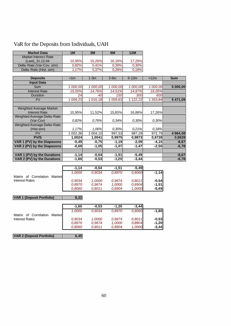
60
VaR for the Deposits from Individuals, UAH Market Data 1M 3M 6M 12M
Market Interes t Rate (Last)_31.12.04 10,95% 15,26% 16,16% 17,26%
Delta -Rate (Var-Cov. sim) 0,82% 0,41% 0,30% 0,30% Delta -Rate (Hist. sim) 1,17% 0,37% 0,26% 0,18%
Deposits <1m 1-3m 3-6m 6-12m >12m Sum
Input Data Sum 1 000,00 1 000,00 1 000,00 1 000,00 1 000,00 5 000,00
Interest Rate 15,00% 14,76% 14,51% 14,87% 16,05% Duration 24 40 150 300 600
FV 1 009,23 1 016,18 1 059,63 1 122,22 1 263,84 5 471,09
Weighted Average Market Interest Rate 10,95% 11,52% 15,83% 16,86% 17,26%
Weighted Average Delta-Rate (Var-Cov) 0,82% 0,76% 0,34% 0,30% 0,30%
Weighted Average Delta-Rate (Hist.sim) 1,17% 1,06% 0,30% 0,21% 0,18%
PV 1 002,36 1 004,10 997,53 987,29 972,79 4 964,08 PV/S 1,0024 1,0041 0,9975 0,9873 0,9728 0,9928
VAR 1 (PV) by the Diapasons -0,49 -0,75 -1,19 -2,09 -4,15 -8,67 VAR 2 (PV) by the Diapasons -0,69 -1,05 -1,07 -1,47 -2,50 -6,78
VAR 1 (PV) by the Durations -1,14 -0,54 -1,51 -5,49 -8,67 VAR 2 (PV) by the Durations -1,60 -0,53 -1,20 -3,44 -6,78
-1,14 -0,54 -1,51 -5,49 1,0000 0,9034 0,8970 0,8060 -1,14 Matrix of Correlation Market Interest Rates 0,9034 1,0000 0,9674 0,8011 -0,54 0,8970 0,9674 1,0000 0,8904 -1,51 0,8060 0,8011 0,8904 1,0000 -5,49 VAR 1 (Deposit Portfolio) 8,32 -1,60 -0,53 -1,20 -3,44 1,0000 0,9034 0,8970 0,8060 -1,60 Matrix of Correlation Market Interest Rates 0,9034 1,0000 0,9674 0,8011 -0,53 0,8970 0,9674 1,0000 0,8904 -1,20 0,8060 0,8011 0,8904 1,0000 -3,44 VAR 2 (Deposit Portfolio) 6,45

61
VaR for the Deposits from Firms, UAH Market Data 1M 3M 6M 12M
Market Interest Rate (Last)_31.12.04 12,36% 14,02% 15,14% 16,89%
Delta-Rate (Var-Cov. sim) 0,83% 0,52% 0,39% 0,40% Delta -Rate (Hist. sim) 0,84% 0,42% 0,30% 0,26%
Deposits <1m 1-3m 3-6m 6-12m >12m Sum
Input Data Sum 1 000,00 1 000,00 1 000,00 1 000,00 1 000,00 5 000,00
Interest Rate 13,00% 15,89% 15,97% 16,47% 15,07% Duration 24 40 150 300 600
FV 1 008,07 1 017,41 1 065,63 1 135,37 1 247,73 5 474,21
Weighted Average Market Interest Rate 12,36% 12,58% 14,73% 16,26% 16,89%
Weighted Average Delta-Rate (Var-Cov) 0,83% 0,79% 0,44% 0,40% 0,40%
Weighted Average Delta-Rate (Hist.sim) 0,84% 0,78% 0,35% 0,28% 0,26%
PV 1 000,37 1 004,29 1 007,12 1 003,12 965,39 4 980,30 PV/S 1,0004 1,0043 1,0071 1,0031 0,9654 0,9961
VAR 1 (PV) by the Diapasons -0,48 -0,77 -1,58 -2,82 -5,43 -11,08 VAR 2 (PV) by the Diapasons -0,49 -0,76 -1,25 -1,98 -3,59 -8,08
VAR 1 (PV) by the Durations -1,15 -0,68 -2,01 -7,24 -11,08 VAR 2 (PV) by the Durations -1,15 -0,56 -1,50 -4,86 -8,08
-1,15 -0,68 -2,01 -7,24 1,0000 0,9715 0,8938 0,7984 -1,15 Matrix of Correlation Market Interest Rates 0,9715 1,0000 0,9618 0,8668 -0,68 0,8938 0,9618 1,0000 0,9522 -2,01 0,7984 0,8668 0,9522 1,0000 -7,24 VAR 1 (Deposit Portfolio) 10,78 -1,15 -0,56 -1,50 -4,86 1,0000 0,9715 0,8938 0,7984 -1,15 Matrix of Correlation Market Interest Rates 0,9715 1,0000 0,9618 0,8668 -0,56 0,8938 0,9618 1,0000 0,9522 -1,50 0,7984 0,8668 0,9522 1,0000 -4,86 VAR 2 (Deposit Portfolio) 7,82
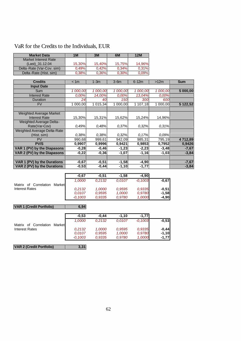
62
VaR for the Credits to the Individuals, EUR Market Data 1M 3M 6M 12M
Market Interest Rate (Last)_31.12.04 15,30% 15,40% 15,75% 14,96%
Delta -Rate (Var-Cov. sim) 0,49% 0,42% 0,34% 0,31% Delta -Rate (Hist. sim) 0,38% 0,36% 0,30% 0,09%
Credits < 1m 1-3m 3-6m 6-12m >12m Sum
Input Date Sum 1 000,00 1 000,00 1 000,00 1 000,00 1 000,00 5 000,00
Interest Rate 0,00% 14,00% 0,00% 13,04% 0,00% Duration 24 40 150 300 600
FV 1 000,00 1 015,34 1 000,00 1 107,18 1 000,00 5 122,52
Weighted Average Market Interest Rate 15,30% 15,31% 15,62% 15,24% 14,96%
Weighted Average Delta-Rate(Var-Cov) 0,49% 0,48% 0,37% 0,32% 0,31%
Weighted Average Delta-Rate (Hist. sim) 0,38% 0,38% 0,32% 0,17% 0,09%
PV 990,68 999,61 942,09 985,31 795,19 4 712,89 PV/S 0,9907 0,9996 0,9421 0,9853 0,7952 0,9426
VAR 1 (PV) by the Diapasons -0,28 -0,46 -1,23 -2,23 -3,48 -7,67 VAR 2 (PV) by the Diapasons -0,22 -0,36 -1,07 -1,16 -1,03 -3,84
VAR 1 (PV) by the Durations -0,67 -0,51 -1,58 -4,90 -7,67 VAR 2 (PV) by the Durations -0,53 -0,44 -1,10 -1,77 -3,84
-0,67 -0,51 -1,58 -4,90 1,0000 0,2132 0,0107 -0,1003 -0,67 Matrix of Correlation Market Interest Rates 0,2132 1,0000 0,9595 0,9335 -0,51 0,0107 0,9595 1,0000 0,9780 -1,58 -0,1003 0,9335 0,9780 1,0000 -4,90 VAR 1 (Credit Portfolio) 6,94 -0,53 -0,44 -1,10 -1,77 1,0000 0,2132 0,0107 -0,1003 -0,53 Matrix of Correlation Market Interest Rates 0,2132 1,0000 0,9595 0,9335 -0,44 0,0107 0,9595 1,0000 0,9780 -1,10 -0,1003 0,9335 0,9780 1,0000 -1,77 VAR 2 (Credit Portfolio) 3,31
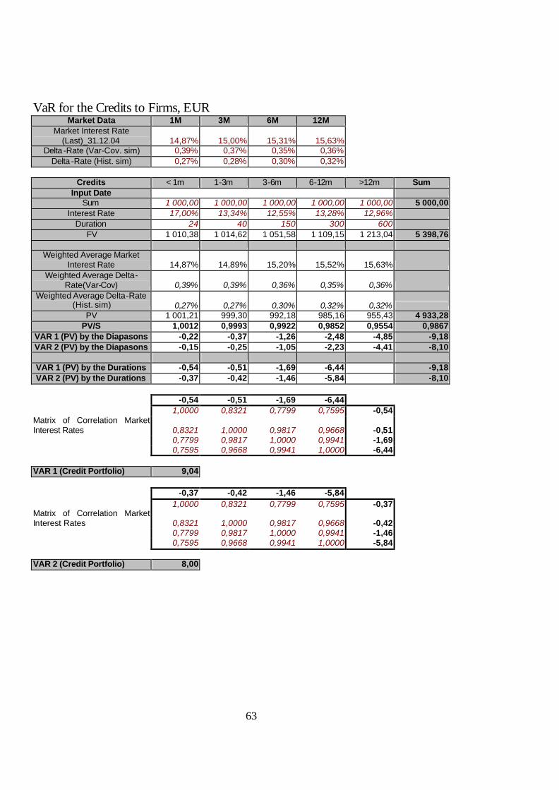
63
VaR for the Credits to Firms, EUR Market Data 1M 3M 6M 12M
Market Interest Rate (Last)_31.12.04 14,87% 15,00% 15,31% 15,63%
Delta -Rate (Var-Cov. sim) 0,39% 0,37% 0,35% 0,36% Delta -Rate (Hist. sim) 0,27% 0,28% 0,30% 0,32%
Credits < 1m 1-3m 3-6m 6-12m >12m Sum
Input Date Sum 1 000,00 1 000,00 1 000,00 1 000,00 1 000,00 5 000,00
Interest Rate 17,00% 13,34% 12,55% 13,28% 12,96% Duration 24 40 150 300 600
FV 1 010,38 1 014,62 1 051,58 1 109,15 1 213,04 5 398,76
Weighted Average Market Interest Rate 14,87% 14,89% 15,20% 15,52% 15,63%
Weighted Average Delta-Rate(Var-Cov) 0,39% 0,39% 0,36% 0,35% 0,36%
Weighted Average Delta-Rate (Hist. sim) 0,27% 0,27% 0,30% 0,32% 0,32%
PV 1 001,21 999,30 992,18 985,16 955,43 4 933,28 PV/S 1,0012 0,9993 0,9922 0,9852 0,9554 0,9867
VAR 1 (PV) by the Diapasons -0,22 -0,37 -1,26 -2,48 -4,85 -9,18 VAR 2 (PV) by the Diapasons -0,15 -0,25 -1,05 -2,23 -4,41 -8,10
VAR 1 (PV) by the Durations -0,54 -0,51 -1,69 -6,44 -9,18 VAR 2 (PV) by the Durations -0,37 -0,42 -1,46 -5,84 -8,10
-0,54 -0,51 -1,69 -6,44 1,0000 0,8321 0,7799 0,7595 -0,54 Matrix of Correlation Market Interest Rates 0,8321 1,0000 0,9817 0,9668 -0,51 0,7799 0,9817 1,0000 0,9941 -1,69 0,7595 0,9668 0,9941 1,0000 -6,44 VAR 1 (Credit Portfolio) 9,04 -0,37 -0,42 -1,46 -5,84 1,0000 0,8321 0,7799 0,7595 -0,37 Matrix of Correlation Market Interest Rates 0,8321 1,0000 0,9817 0,9668 -0,42 0,7799 0,9817 1,0000 0,9941 -1,46 0,7595 0,9668 0,9941 1,0000 -5,84 VAR 2 (Credit Portfolio) 8,00

64
VaR for the Deposits from Individuals, EUR Market Data 1M 3M 6M 12M
Market Interest Rate (Last)_31.12.04 5,31% 7,59% 8,25% 9,51%
Delta -Rate (Var-Cov. sim) 0,59% 0,44% 0,33% 0,36% Delta -Rate (Hist. sim) 1,05% 0,26% 0,23% 0,34%
Deposits < 1m 1-3m 3-6m 6-12m >12m Sum
Input Date Sum 1 000,00 1 000,00 1 000,00 1 000,00 1 000,00 5 000,00
Interest Rate 5,50% 6,27% 6,25% 5,52% 6,03% Duration 24 40 150 300 600
FV 1 003,53 1 006,87 1 025,68 1 045,37 1 099,12 5 180,58
Weighted Average Market Interest Rate 5,31% 5,61% 8,01% 9,06% 9,51%
Weighted Average Delta-Rate(Var-Cov) 0,59% 0,57% 0,37% 0,35% 0,36%
Weighted Average Delta-Rate (Hist. sim) 1,05% 0,95% 0,24% 0,30% 0,34%
PV 1 000,12 1 000,86 993,72 973,46 946,65 4 914,82 PV/S 1,0001 1,0009 0,9937 0,9735 0,9467 0,9830
VAR 1 (PV) by the Diapasons -0,37 -0,60 -1,39 -2,55 -5,10 -10,00 VAR 2 (PV) by the Diapasons -0,66 -0,98 -0,91 -2,19 -4,79 -9,53
VAR 1 (PV) by the Durations -0,89 -0,59 -1,79 -6,73 -10,00 VAR 2 (PV) by the Durations -1,51 -0,46 -1,36 -6,19 -9,53
-0,89 -0,59 -1,79 -6,73 1,0000 0,8949 0,8495 0,8656 -0,89 Matrix of Correlation Market Interest Rates 0,8949 1,0000 0,9829 0,9801 -0,59 0,8495 0,9829 1,0000 0,9937 -1,79 0,8656 0,9801 0,9937 1,0000 -6,73 VAR 1 (Deposit Portfolio) 9,87 -1,51 -0,46 -1,36 -6,19 1,0000 0,8949 0,8495 0,8656 -1,51 Matrix of Correlation Market Interest Rates 0,8949 1,0000 0,9829 0,9801 -0,46 0,8495 0,9829 1,0000 0,9937 -1,36 0,8656 0,9801 0,9937 1,0000 -6,19 VAR 2 (Deposit Portfolio) 9,34

65
VaR for the Deposits from the Firms, EUR Market Data 1M 3M 6M 12M
Market Interest Rate (Last)_31.12.04 6,13% 7,16% 8,04% 9,05%
Delta -Rate (Var-Cov. sim) 0,41% 0,42% 0,38% 0,31% Delta -Rate (Hist. sim) 0,30% 2,00% 0,34% 0,29%
Deposits < 1m 1-3m 3-6m 6-12m >12m Sum
Input Date Sum 1 000,00 1 000,00 1 000,00 1 000,00 1 000,00 5 000,00
Interest Rate 5,00% 5,92% 8,38% 8,00% 0,00% Duration 24 40 150 300 600
FV 1 003,21 1 006,49 1 034,44 1 065,75 1 000,00 5 109,89
Weighted Average Market Interest Rate 6,13% 6,27% 7,72% 8,69% 9,05%
Weighted Average Delta-Rate(Var-Cov) 0,41% 0,41% 0,40% 0,34% 0,31%
Weighted Average Delta-Rate (Hist. sim) 0,30% 0,53% 0,95% 0,31% 0,29%
PV 999,30 999,81 1 003,31 995,22 867,26 4 864,90 PV/S 0,9993 0,9998 1,0033 0,9952 0,8673 0,9730
VAR 1 (PV) by the Diapasons -0,25 -0,42 -1,51 -2,53 -4,06 -8,78 VAR 2 (PV) by the Diapasons -0,19 -0,54 -3,63 -2,30 -3,73 -10,40
VAR 1 (PV) by the Durations -0,62 -0,61 -1,87 -5,68 -8,78 VAR 2 (PV) by the Durations -0,66 -1,41 -3,13 -5,21 -10,40
-0,62 -0,61 -1,87 -5,68 1,0000 0,8244 0,8224 0,7873 -0,62 Matrix of Correlation Market Interest Rates 0,8244 1,0000 0,9954 0,9808 -0,61 0,8224 0,9954 1,0000 0,9766 -1,87 0,7873 0,9808 0,9766 1,0000 -5,68 VAR 1 (Deposit Portfolio) 8,62 -0,66 -1,41 -3,13 -5,21 1,0000 0,8244 0,8224 0,7873 -0,66 Matrix of Correlation Market Interest Rates 0,8244 1,0000 0,9954 0,9808 -1,41 0,8224 0,9954 1,0000 0,9766 -3,13 0,7873 0,9808 0,9766 1,0000 -5,21 VAR 2 (Deposit Portfolio) 10,22

66
VaR for the Credits to Individuals, USD Market Data 1M 3M 6M 12M
Market Interest Rate (Last)_31.12.04 15,73% 15,90% 16,23% 15,90%
Delta -Rate (var-cov. sim.) 0,29% 0,24% 0,20% 0,21% Delta -Rate (Hist.sim.) 0,22% 0,20% 0,20% 0,25%
Credits <1m 1-3m 3-6m 6-12m <12m Sum
Input Data Sum 1 000,00 1 000,00 1 000,00 1 000,00 1 000,00 5 000,00
Interest Rate 0,00% 11,22% 12,52% 13,16% 0,00% Duration 24 40 150 300 600
FV 1 000,00 1 012,30 1 051,45 1 108,16 1 000,00 5 171,91
Weighted Average Market Interest Rate 15,73% 15,75% 16,11% 16,02% 15,90%
Weighted Average Delta-Rate (Var-Cov) 0,29% 0,29% 0,21% 0,20% 0,21%
Weighted Average Delta-Rate (Hist.sim.) 0,22% 0,22% 0,20% 0,23% 0,25%
PV 990,44 996,20 988,85 980,77 784,62 4 740,88 PV/S 0,9904 0,9962 0,9889 0,9808 0,7846 0,9482
VAR 1 (PV) by the Diapasons -0,17 -0,27 -0,75 -1,42 -2,30 -4,90 VAR 2 (PV) by the Diapasons -0,12 -0,20 -0,70 -1,61 -2,78 -5,42
VAR 1 (PV) by the Durations -0,40 -0,31 -0,98 -3,20 -4,90 VAR 2 (PV) by the Durations -0,30 -0,28 -1,02 -3,82 -5,42
-0,40 -0,31 -0,98 -3,20 1,0000 0,8907 0,8890 0,8473 -0,40 Matrix of Correlation Market Interest Rates 0,8907 1,0000 0,9915 0,9859 -0,31 0,8890 0,9915 1,0000 0,9919 -0,98 0,8473 0,9859 0,9919 1,0000 -3,20 VAR 1 (Credit Portfolio) 4,84 -0,30 -0,28 -1,02 -3,82 1,0000 0,8907 0,8890 0,8473 -0,30 Matrix of Correlation Market Interest Rates 0,8907 1,0000 0,9915 0,9859 -0,28 0,8890 0,9915 1,0000 0,9919 -1,02 0,8473 0,9859 0,9919 1,0000 -3,82 VAR 2 (Credit Portfolio) 5,37

67
VaR for the Credits to Firms, USD Market Data 1M 3M 6M 12M
Market Interest Rate (Last)_31.12.04 15,65% 15,83% 16,11% 16,43%
Delta -Rate (var-cov. sim.) 0,25% 0,21% 0,18% 0,17% Delta -Rate (Hist.sim.) 0,22% 0,22% 0,18% 0,19%
Credits <1m 1-3m 3-6m 6-12m <12m Sum
Input Data Sum 1 000,00 1 000,00 1 000,00 1 000,00 1 000,00 5 000,00
Interest Rate 12,20% 13,73% 13,59% 13,13% 12,52% Duration 24 40 150 300 600
FV 1 007,60 1 015,05 1 055,85 1 107,92 1 205,81 5 392,22
Weighted Average Market Interest Rate 15,65% 15,67% 16,01% 16,32% 16,43%
Weighted Average Delta-Rate (Var-Cov) 0,25% 0,25% 0,19% 0,17% 0,17%
Weighted Average Delta-Rate (Hist.sim.) 0,22% 0,22% 0,19% 0,19% 0,19%
PV 998,01 998,98 993,35 978,50 939,03 4 907,86 PV/S 0,9980 0,9990 0,9933 0,9785 0,9390 0,9816
VAR 1 (PV) by the Diapasons -0,14 -0,23 -0,66 -1,19 -2,25 -4,47 VAR 2 (PV) by the Diapasons -0,12 -0,20 -0,68 -1,30 -2,56 -4,86
VAR 1 (PV) by the Durations -0,34 -0,27 -0,84 -3,01 -4,47 VAR 2 (PV) by the Durations -0,30 -0,28 -0,89 -3,39 -4,86
-0,34 -0,27 -0,84 -3,01 1,0000 0,8499 0,6951 0,7345 -0,34 Matrix of Correlation Market Interest Rates 0,8499 1,0000 0,9391 0,9487 -0,27 0,6951 0,9391 1,0000 0,9922 -0,84 0,7345 0,9487 0,9922 1,0000 -3,01 VAR 1 (Credit Portfolio) 4,37 -0,30 -0,28 -0,89 -3,39 1,0000 0,8499 0,6951 0,7345 -0,30 Matrix of Correlation Market Interest Rates 0,8499 1,0000 0,9391 0,9487 -0,28 0,6951 0,9391 1,0000 0,9922 -0,89 0,7345 0,9487 0,9922 1,0000 -3,39 VAR 2 (Credit Portfolio) 4,77

68
VaR for the Deposits from Individuals, USD Market Data 1M 3M 6M 12M
Market Interest Rate (Last)_31.12.04 5,36% 8,62% 9,32% 10,46%
Delta -Rate (var-cov. sim.) 0,46% 0,35% 0,20% 0,20% Delta -Rate (Hist.sim.) 0,99% 0,20% 0,10% 0,10%
Deposits <1m 1-3m 3-6m 6-12m <12m Sum
Input Data Sum 1 000,00 1 000,00 1 000,00 1 000,00 1 000,00 5 000,00
Interest Rate 6,70% 6,84% 6,86% 6,21% 8,52% Duration 24 40 150 300 600
FV 1 004,27 1 007,50 1 028,19 1 051,04 1 140,05 5 231,06
Weighted Average Market Interest Rate 5,36% 5,79% 9,06% 10,05% 10,46%
Weighted Average Delta-Rate (Var-Cov) 0,46% 0,45% 0,26% 0,20% 0,20%
Weighted Average Delta-Rate (Hist.sim.) 0,99% 0,88% 0,14% 0,10% 0,10%
PV 1 000,83 1 001,30 992,18 971,48 968,06 4 933,85 PV/S 1,0008 1,0013 0,9922 0,9715 0,9681 0,9868
VAR 1 (PV) by the Diapasons -0,29 -0,46 -0,97 -1,46 -2,86 -6,03 VAR 2 (PV) by the Diapasons -0,62 -0,91 -0,52 -0,75 -1,49 -4,29
VAR 1 (PV) by the Durations -0,69 -0,42 -1,14 -3,79 -6,03 VAR 2 (PV) by the Durations -1,41 -0,31 -0,60 -1,97 -4,29
-0,69 -0,42 -1,14 -3,79 1,0000 0,8535 0,8080 0,8284 -0,69 Matrix of Correlation Market Interest Rates 0,8535 1,0000 0,9863 0,9824 -0,42 0,8080 0,9863 1,0000 0,9951 -1,14 0,8284 0,9824 0,9951 1,0000 -3,79 VAR 1 (Deposit Portfolio) 5,92 -1,41 -0,31 -0,60 -1,97 1,0000 0,8535 0,8080 0,8284 -1,41 Matrix of Correlation Market Interest Rates 0,8535 1,0000 0,9863 0,9824 -0,31 0,8080 0,9863 1,0000 0,9951 -0,60 0,8284 0,9824 0,9951 1,0000 -1,97 VAR 2 (Deposit Portfolio) 4,12

69
VaR for the Deposits from Firms, USD Market Data 1M 3M 6M 12M
Market Interest Rate (Last)_31.12.04 6,35% 7,48% 8,29% 9,61%
Delta -Rate (var-cov. sim.) 0,43% 0,34% 0,30% 0,26% Delta -Rate (Hist.sim.) 0,34% 0,22% 0,21% 0,11%
Deposits <1m 1-3m 3-6m 6-12m <12m Sum
Input Data Sum 1 000,00 1 000,00 1 000,00 1 000,00 1 000,00 5 000,00
Interest Rate 7,30% 6,41% 7,44% 9,56% 0,00% Duration 24 40 150 300 600
FV 1 004,64 1 007,02 1 030,58 1 078,58 1 000,00 5 120,82
Weighted Average Market Interest Rate 6,35% 6,50% 7,99% 9,14% 9,61%
Weighted Average Delta-Rate (Var-Cov) 0,43% 0,42% 0,31% 0,28% 0,26%
Weighted Average Delta-Rate (Hist.sim.) 0,34% 0,33% 0,21% 0,14% 0,11%
PV 1 000,58 1 000,10 998,52 1 003,79 859,99 4 862,98 PV/S 1,0006 1,0001 0,9985 1,0038 0,8600 0,9726
VAR 1 (PV) by the Diapasons -0,27 -0,43 -1,20 -2,08 -3,36 -7,33 VAR 2 (PV) by the Diapasons -0,21 -0,34 -0,81 -1,09 -1,39 -3,84
VAR 1 (PV) by the Durations -0,64 -0,50 -1,50 -4,69 -7,33 VAR 2 (PV) by the Durations -0,51 -0,34 -0,91 -2,09 -3,84
-0,64 -0,50 -1,50 -4,69 1,0000 0,8744 0,8473 0,8311 -0,64 Matrix of Correlation Market Interest Rates 0,8744 1,0000 0,9904 0,9722 -0,50 0,8473 0,9904 1,0000 0,9792 -1,50 0,8311 0,9722 0,9792 1,0000 -4,69 VAR 1 (Deposit Portfolio) 7,20 -0,51 -0,34 -0,91 -2,09 1,0000 0,8744 0,8473 0,8311 -0,51 Matrix of Correlation Market Interest Rates 0,8744 1,0000 0,9904 0,9722 -0,34 0,8473 0,9904 1,0000 0,9792 -0,91 0,8311 0,9722 0,9792 1,0000 -2,09 VAR 2 (Deposit Portfolio) 3,76
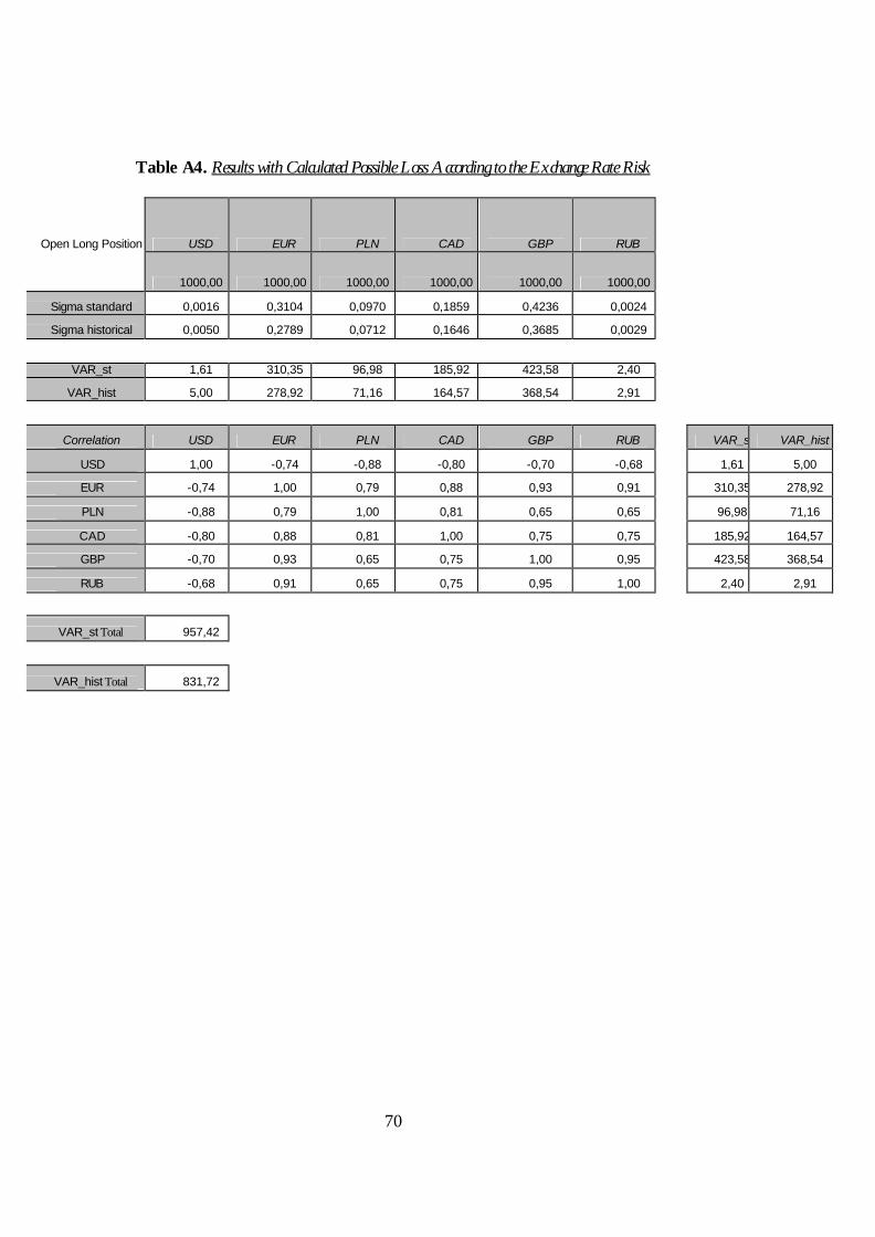
70
Table A4. Results with Calculated Possible Loss According to the Exchange Rate Risk
Open Long Position USD EUR PLN CAD GBP RUB
1000,00 1000,00 1000,00 1000,00 1000,00 1000,00
Sigma standard 0,0016 0,3104 0,0970 0,1859 0,4236 0,0024
Sigma historical 0,0050 0,2789 0,0712 0,1646 0,3685 0,0029
VAR_st 1,61 310,35 96,98 185,92 423,58 2,40
VAR_hist 5,00 278,92 71,16 164,57 368,54 2,91
Correlation USD EUR PLN CAD GBP RUB VAR_st VAR_hist
USD 1,00 -0,74 -0,88 -0,80 -0,70 -0,68 1,61 5,00
EUR -0,74 1,00 0,79 0,88 0,93 0,91 310,35 278,92
PLN -0,88 0,79 1,00 0,81 0,65 0,65 96,98 71,16
CAD -0,80 0,88 0,81 1,00 0,75 0,75 185,92 164,57
GBP -0,70 0,93 0,65 0,75 1,00 0,95 423,58 368,54
RUB -0,68 0,91 0,65 0,75 0,95 1,00 2,40 2,91
VAR_st Total 957,42
VAR_hist Total 831,72