Convolutional Neural Networks Analyzed via

Convolutional Sparse Coding

Vardan Papyan*, Yaniv Romano*, Michael Elad

March 7, 2018

Abstract

In recent years, deep learning and in particular convolutional neuralnetworks (CNN) have led to some remarkable results in various fields.In this scheme, an input signal is convolved with learned filters and anon-linear point wise function is then applied on the response map. Of-tentimes, an additional non-linear step, termed pooling, is applied on theoutcome. The obtained result is then fed to another layer that operatessimilarly, thereby creating a multi-layered convolutional architecture. De-spite its marvelous empirical success, a clear and profound theoreticalunderstanding of this scheme, termed forward pass, is still lacking.

Another popular paradigm in recent years is the sparse representationmodel, where one assumes that a signal can be described as the multipli-cation of a dictionary by a sparse vector. A special case of this model thathas drawn interest in recent years is the convolutional sparse coding (CSC)model, in which the dictionary assumes a specific structure – a union ofbanded and Circulant matrices. Unlike CNN, sparsity inspired models areaccompanied by a thorough theoretical analysis. Indeed, such a study ofthe CSC model and its properties has been performed in [1,2], establishingthis model as a reliable and stable alternative to the commonly practicedpatch-based processing.

In this work we leverage the recent study of the CSC model, in orderto bring a fresh view to CNN with a deeper theoretical understanding.Our analysis relies on the observation that akin to the original signal, thesparse representation itself can also be modeled as a sparse compositionof yet another set of atoms from a convolutional dictionary. This con-struction, which can clearly be extended to more than two layers, resultsin the definition of the multi-layered convolutional sparse model, which istightly related to deconvolutional networks. Several questions arise fromthe above model:

∗The authors contributed equally to this work.V. Papyan is with the Computer Science Department, the Technion – Israel Institute of Tech-nology, Technion City, Haifa 32000, Israel. E-mail address: vardanp@campus.technion.ac.il.Y. Romano is with the Department of Electrical Engineering, Technion. E-mail address:yromano@tx.technion.ac.il. M. Elad is with the Computer Science Department, Technion.E-mail address: elad@cs.technion.ac.il.

1

arX

iv:1

607.

0819

4v1

[st

at.M

L]

27

Jul 2

016

1. What is the relation between CNN and the multi-layered convolu-tional sparse model?

2. In particular, can we interpret the forward pass of CNN as a simplepursuit algorithm?

3. If so, can we leverage this connection to provide a sound theoreticalfoundation for the forward pass of CNN? Specifically, is this algo-rithm guaranteed to succeed assuming certain conditions are met?Is it stable to slight perturbations in its input?

4. Lastly, can we leverage the answers to the above questions, andpropose alternatives to CNN’s forward pass?

The answers to these questions are the main concern of this paper.

1 Introduction

Deep learning [3], and in particular CNN [4–6], has gained a copious amount ofattention in recent years as it has led to many state-of-the-art results spanningthrough many fields – including speech recognition [7–9], computer vision [10–12], signal and image processing [13–16], to name a few. In the context ofthe CNN, the forward pass is a multi-layered scheme that provides an end-to-end mapping, from an input signal to some desired output. Each stage of thisalgorithm corresponds to a certain layer in the network, and consists of threesteps. The first convolves the input to the layer with a set of learned filters,resulting in a set of feature (or kernel) maps. These then undergo a point wisenon-linear function, in a second step, often resulting in a sparse outcome [17].A third (and optional) nonlinear down-sampling step, termed pooling, is thenapplied on the result in order to reduce its dimensions. The output of this layeris then fed into another one, thus forming the multi-layered structure.

A few preliminary theoretical results for this scheme were recently suggested.In [18] the wavelet scattering transform was proposed, suggesting to replace thelearned filters in the CNN with predefined wavelet functions. Interestingly,the features obtained from this network were shown to be invariant to varioustransformations such as translations and rotations. Other works have studiedthe properties of deep and fully connected networks under the assumption ofindependent identically distributed random weights [19–23]. In particular, in[19] deep neural networks were proven to preserve the metric structure of theinput data as it propagates throughout the layers of the network. This, in turn,was shown to allow a stable recovery of the data from the features obtainedfrom the network. On the contrary, in this work we do not restrict ourselves topredefined filters, nor to random weights. Moreover, we study both the CNNarchitecture and the fully connected one, where the latter can be interpreted asa special case of the former.

Another prominent paradigm is the sparse representation, being one of themost popular choices for a prior in the signal and image processing communi-ties, and leading to exceptional results in various applications [24–28]. In this

2

framework, one assumes that a signal can be represented as a linear combina-tion of a few columns (called atoms) from a matrix termed a dictionary. Putdifferently, the signal is equal to a multiplication of a dictionary by a sparsevector. The task of retrieving the sparsest representation of a signal over adictionary is called sparse coding or pursuit. Over the years, various algorithmswere proposed to tackle it, such as the thresholding algorithm [29] and its it-erative variant [30]. This model has been commonly used for modeling localpatches extracted from global signals due to both computational and theoreti-cal difficulties [24,25,28, 31,32]. However, in recent years an alternative to thispatch-based processing has emerged in the form of the convolutional sparse cod-ing (CSC) model [1,2,33–37]. This circumvents the aforementioned limitationsby imposing a special structure – a union of banded and Circulant matrices –on the dictionary involved. The traditional sparse model has been extensivelystudied over the past two decades [29, 38]. And similarly, the recent convolu-tional extension was analyzed in [1,2], shedding light on the theoretical aspectsof this model.

In this work we aim to provide a new perspective on CNN with a clear andprofound theoretical understanding. Our approach builds upon the observationthat similar to the original signal, the representation vector itself also admits aconvolutional sparse representation. As such, it can be modeled as a superposi-tion of atoms, taken from a different convolutional dictionary. This rationale canbe extended to several layers, leading to the definition of our proposed multi-layered convolutional sparse model. Leveraging the recent analysis of the CSC,we provide a theoretical study of this novel model and its associated pursuits,namely the layered thresholding algorithm and its iterative variant.

Our analysis reveals the relation between the CNN and the multi-layeredconvolutional sparse model, showing that the forward pass of the CNN is infact identical to our proposed pursuit – the layered thresholding algorithm.This connection is of significant importance since it provides guarantees forthe success of the forward pass by leveraging those of the layered thresholdingalgorithm. Specifically, we show that the forward pass is guaranteed to recoveran estimate of the underlying representations of an input signal, assuming theseare sparse in a local sense. Moreover, considering a setting where a norm-bounded noise is added to the signal, we show that such a mild corruptionin the input results in a bounded perturbation in the output – indicating thestability of the CNN. Lastly, we leverage the answers to the above questions,and propose an alternative to the commonly used forward pass algorithm, whichis tightly connected to deconvolutional [39] and recurrent networks [40].

This paper is organized as follows. In Section 2 we review the basics ofboth the CNN and the Sparse-Land model. We then define the proposed multi-layered convolutional sparse model in Section 3, together with its correspondingdeep coding problem. In Section 4, we aim to solve this using the layeredthresholding algorithm, which is shown to be equivalent to the forward pass ofthe CNN. Next, having established the importance of our model, we proceed toits analysis in Section 5. Standing on these theoretical grounds, we then proposein Section 6 an improved pursuit, termed the layered iterative thresholding,

3

(a) A convolutional matrix.

(b) A concatenation of banded and Circulant matrices.

Figure 1: The two facets of the convolutional structure.

which we envision as a promising future direction in deep learning. We revisitthe assumptions of our model in Section 7, linking it to double sparsity anddeconvolutional networks.

2 Background

This section is divided into two parts: The first is dedicated to providing asimple mathematical formulation of the CNN and the forward pass, while thesecond reviews the Sparse-Land model and its various extensions.

2.1 Deep Learning - Convolutional Neural Networks

The fundamental algorithm of deep learning is the forward pass, employed bothin the training and the inference stages. The first step of this algorithm con-volves an input (one dimensional) signal X ∈ RN with a set of m1 learnedfilters of length n0, creating m1 feature (or kernel) maps. Equally, this convo-lution can be written as a matrix-vector multiplication, WT

1 X ∈ RNm1 , whereW1 ∈ RN×Nm1 is a matrix containing in its columns the m1 filters in all shifts.This structure, also known as a convolutional matrix, is depicted in Figure1a. A pointwise nonlinear function is then applied on the sum of the obtainedfeature maps WT

1 X and a bias term denoted by b1 ∈ RNm1 . Many possi-ble functions were proposed over the years, the most popular one being theRectifier Linear Unit (ReLU) [6, 17], formally defined as ReLU(z) = max(z, 0).By cascading the basic block of convolutions followed by a nonlinear function,Z1 = ReLU(WT

1 X + b1), a multi-layer structure of depth K is constructed.Formally, for two layers this is given by

f(X, Wi2i=1, bi2i=1) = Z2 = ReLU

(WT

2 ReLU(

WT1 X + b1

)+b2

), (1)

where W2 ∈ RNm1×Nm2 is a convolutional matrix (up to a small modificationdiscussed below) constructed from m2 filters of length n1m1 and b2 ∈ RNm2 is

4

its corresponding bias. Although the two layers considered here can be readilyextended to a much deeper configuration, we defer this to a later stage.

By changing the order of the columns in the convolutional matrix, one canobserve that it can be equally viewed as a concatenation of banded and Cir-culant1 matrices, as depicted in Figure 1b. Using this observation, the abovedescription for one dimensional signals can be extended to images, with the ex-ception that now every Circulant matrix is replaced by a block Circulant withCirculant blocks one.

An illustration of the forward pass algorithm is presented in Figure 2a and2b. In Figure 2a one can observe that W2 is not a regular convolutional matrixbut a stride one, since it shifts local filters by skipping m1 entries at a time. Thereason for this becomes apparent once we look at Figure 2b; the convolutionsof the second layer are computed by shifting the filters of W2 that are of size√n1 ×

√n1 × m1 across N places, skipping m1 indices at a time from the√

N ×√N ×m1-sized array. A matrix obeying this structure is called a stride

convolutional matrix.Thus far, we have presented the basic structure of CNN. However, oftentimes

an additional non-linear function, termed pooling, is employed on the resultingfeature map obtained by the ReLU operator. In essence, this step summarizeseach si-dimensional spatial neighborhood from the i-th kernel map Zi by re-placing it with a single value. If the neighborhoods are non-overlapping, forexample, this results in the down-sampling of the feature map by a factor ofsi. The most widely used variant of the above is the max pooling [6,11], whichpicks the maximal value of each neighborhood. In [41] it was shown that thisoperator can be replaced by a convolutional layer with increased stride withoutloss in performance in several image classification tasks. Moreover, the currentstate-of-the-art in image recognition is obtained by the residual network [12],which does not employ any pooling steps. As such, we defer the analysis of thisoperator to a follow-up work.

In the context of classification, for example, the output of the last layeris fed into a simple classifier that attempts to predict the label of the inputsignal X, denoted by h(X). Given a set of signals Xjj , the task of learningthe parameters of the CNN – including the filters WiKi=1, the biases biKi=1

and the parameters of the classifier U – can be formulated in the followingminimization problem

minWiKi=1,biKi=1,U

∑j

`(h(Xj),U, f

(Xj , WiKi=1, biKi=1

) ). (2)

This optimization task seeks for the set of parameters that minimize the meanof the loss function `, representing the price incurred when classifying the signalX incorrectly. The input for ` is the true label h(X) and the one estimated byemploying the classifier defined by U on the final layer of the CNN given by

1We shall assume throughout this paper that boundaries are treated by a periodic contin-uation, which gives rise to the cyclic structure.

5

𝑚1 * + + * =

𝐖2T ∈ ℝ𝑁𝑚2×𝑁𝑚1

𝐖1T ∈ ℝ𝑁𝑚1×𝑁

𝐗 ∈ ℝ𝑁

𝐛1 ∈ ℝ𝑁𝑚1

𝐛2 ∈ ℝ𝑁𝑚2 𝐙2 ∈ ℝ

𝑁𝑚2

ReLU

𝑛1𝑚1

𝑚1 𝑛0

𝑚2

ReLU

(a) An illustration of Equation (1) for a one dimensional signal X.

𝑁

𝑁

𝐗

𝑚1

𝑁

𝑁

𝑛0

𝑛0 𝐖1

𝑚2 𝑁

𝑁

𝑛1

𝑛1

𝐖2

(b) The evolution of an image X throughout the CNN. Notice that the numberof channels in X is equal to one and as such m0 = 1.

Figure 2: The forward pass algorithm for a one dimensional signal (a) and animage (b).

f(X, WiKi=1, biKi=1

). Similarly one can tackle various other problems, e.g.

regression or prediction.In the remainder of this work we shall focus on the feature extraction process

and assume that the parameters of the CNN model are pre-trained and fixed.These, for example, could have been obtained by minimizing the above objectivevia the backpropagation algorithm and the stochastic gradient descent, as in theVGG network [11].

2.2 Sparse-Land

This section presents an overview of the Sparse-Land model and its many exten-sions. We start with the traditional sparse representation and the core problem

6

it aims to solve, and then proceed to its nonnegative variant. Next, we continueto the dictionary learning task both in the unsupervised and supervised cases.Finally, we describe the recent CSC model, which will lead us in the next sectionto the proposal of the multi-layered convolutional sparse model. This, in turn,will naturally connect the realm of sparsity to that of the CNN.

2.2.1 Sparse Representation

In the sparse representation model one assumes a signal X ∈ RN can be de-scribed as a multiplication of a matrix D ∈ RN×M , also called a dictionary, by asparse vector Γ ∈ RM . Equally, the signal X can be seen as a linear combinationof a few columns from the dictionary D, coined atoms.

For a fixed dictionary, given a signal X, the task of recovering its sparsestrepresentation Γ is called sparse coding, or simply pursuit, and it attempts tosolve the following problem [29,42,43]:

(P0) : minΓ‖Γ‖0 s.t. DΓ = X, (3)

where we have denoted by ‖Γ‖0 the number of non-zeros in Γ. The above hasa convex relaxation in the form of the Basis-Pursuit (BP) problem [42, 44, 45],formally defined as

(P1) : minΓ‖Γ‖1 s.t. DΓ = X. (4)

Many questions arise from the above two defined problems. For instance, givena signal X, is its sparsest representation unique? Assuming that such a uniquesolution exists, can it be recovered using practical algorithms such as the Orthog-onal Matching Pursuit (OMP) [46,47] and the BP [30,44]? The answers to thesequestions were shown to be positive under the assumption that the number of

non-zeros in Γ is not too high and in particular less than 12

(1 + 1

µ(D)

)[42,43,48].

The quantity µ(D) is the mutual-coherence of the dictionary D, being the max-imal inner product of two atoms extracted from it2. Formally, we can write

µ(D) = maxi 6=j|dTi dj |.

Tighter conditions, relying on sharper characterizations of the dictionary, werealso suggested in the literature [49,49–51]. However, at this point, we shall notdwell on these.

One of the simplest approaches for tackling the P0 and P1 problems is viathe hard and soft thresholding algorithms, respectively. These operate by com-puting the inner products between the signal X and all the atoms in D andthen choosing the atoms corresponding to the highest responses. This can bedescribed as solving, for some scalar β, the following problems:

minΓ

1

2‖Γ−DTX‖22 + β‖Γ‖0

2Hereafter, we assume that the atoms are normalized to a unit `2 norm.

7

for the P0, or

minΓ

1

2‖Γ−DTX‖22 + β‖Γ‖1, (5)

for the P1. The above are simple projection problems that admit a closed-formsolution in the form3 of Hβ(DTX) or Sβ(DTX), where we have defined thehard thresholding operator Hβ(·) by

Hβ(z) =

z, z < −β0, −β ≤ z ≤ βz, β < z,

and the soft thresholding operator Sβ(·) by

Sβ(z) =

z + β, z < −β0, −β ≤ z ≤ βz − β, β < z.

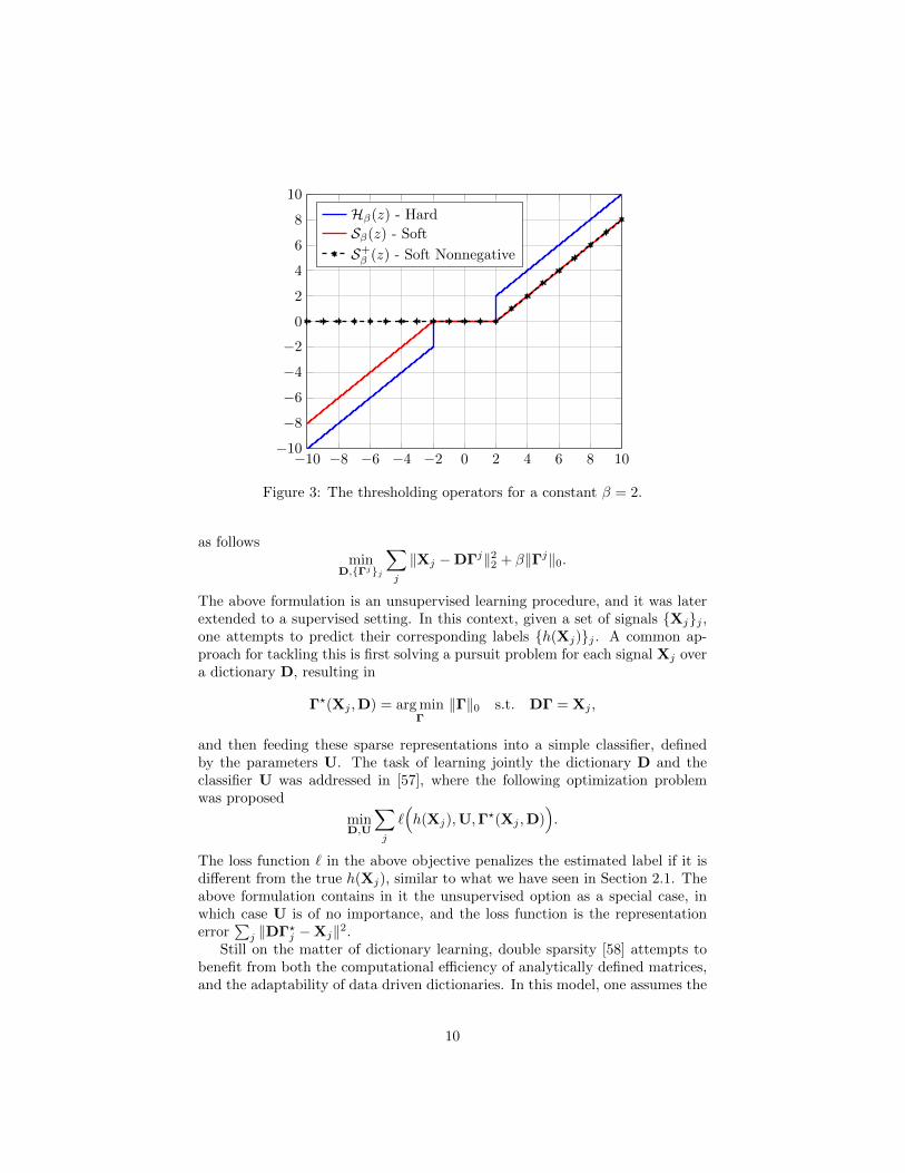
Both of the above, depicted in Figure 3, nullify small entries and thus promote asparse solution. However, while the hard thresholding operator does not modifylarge coefficients (in absolute value), the soft thresholding does, by contractingthese to zero. This inherent limitation of the soft version will appear later onin our theoretical analysis.

As for the theoretical guarantees of the success of the simple thresholdingalgorithms; these depend on the properties of D and on the ratio between themaximal and minimal coefficients in absolute value in the underlying solutionΓ, and thus are weaker when compared to those found for the OMP and theBP [42,43,48]. Indeed, for the case of unitary dictionary, the above thresholdingmethods are optimal. Moreover, under some conditions, both operators can beguaranteed to find the true support of Γ along with an approximation of itstrue coefficients. In order to obtain a better estimation of these, once the truesupport is found using the these algorithms, a projection of the signal ontothe chosen atoms is usually employed by solving a least squares problem (thisprocess is termed debiasing [29]). This, in turn, results in the recovery of thetrue support, and a more accurate identification of the non-zero values.

2.2.2 Nonnegative Sparse Coding

The nonnegative sparse representation model assumes a signal can be decom-posed into a multiplication of a dictionary and a nonnegative sparse vector. Anatural question arising from this is whether such a modification to the originalSparse-Land model affects its expressiveness. To address this, we hereby providea simple reduction from the original sparse representation to the nonnegativeone.

3The curious reader may identify the relation between the notations used here and theones in the previous subsection.

8

Consider a signal X = DΓ, where the signs of the entries in Γ are unre-stricted. Notice that this can be equally written as

X = DΓP + (−D)(−ΓN ),

where we have split the vector Γ to its positive coefficients, ΓP , and its negativeones, ΓN . Since the coefficients in ΓP and −ΓN are all positive, one can thusassume the signal X admits a non-negative sparse representation over the dictio-nary [D,−D] with the vector [ΓP ,−ΓN ]

T. Thus, restricting the coefficients in

the sparsity inspired model to be nonnegative does not change its representationpower.

Similar to the original model, in the nonnegative case, one could solve theassociated pursuit problem by employing a soft thresholding algorithm. How-ever, in this case a constraint must be added to the optimization problem inEquation (5), forcing the outcome to be positive, i.e.,

minΓ

1

2‖Γ−DTX‖22 + β‖Γ‖1 s.t. Γ ≥ 0.

Since the above is a simple projection problem (onto the `1 ball constrainedto positive entries), it admits a closed-form solution S+

β (DTX), where we have

defined the soft nonnegative thresholding operator S+β (·) as

S+β (z) =

0, z ≤ βz − β, β < z.

Remarkably, the above function satisfies

S+β (z) = max(z − β, 0) = ReLU(z − β).

In other words, the ReLU and the soft nonnegative thresholding operators areequal, a fact that will prove to be important later in our work. We should notethat a similar conclusion was reached in [52]. To summarize this discussion, wedepict in Figure 3 the hard, soft, and nonnegative soft thresholding operators.

2.2.3 Unsupervised and Task Driven Dictionary Learning

At first, the dictionaries employed in conjunction with the sparsity inspiredmodel were analytically defined matrices, such as the wavelet and the Fourier[53–56]. Although the sparse coding problem under these can be done very effi-ciently, over the years many have shifted to a data driven approach – adaptingthe dictionary D to a set of training signals at hand via some learning proce-dure. This was empirically shown to lead to sparser representations and thusbetter overall performance, however at the cost of complicating the involvedpursuit. Note that the dictionary is usually chosen to be redundant (havingmore columns than rows), in order to enrich its expressiveness. The task oflearning a dictionary for representing a set of signals Xjj can be formulated

9

−10 −8 −6 −4 −2 0 2 4 6 8 10−10

−8

−6

−4

−2

0

2

4

6

8

10

Hβ(z) - Hard

Sβ(z) - Soft

S+β (z) - Soft Nonnegative

Figure 3: The thresholding operators for a constant β = 2.

as followsmin

D,Γjj

∑j

‖Xj −DΓj‖22 + β‖Γj‖0.

The above formulation is an unsupervised learning procedure, and it was laterextended to a supervised setting. In this context, given a set of signals Xjj ,one attempts to predict their corresponding labels h(Xj)j . A common ap-proach for tackling this is first solving a pursuit problem for each signal Xj overa dictionary D, resulting in

Γ?(Xj ,D) = arg minΓ

‖Γ‖0 s.t. DΓ = Xj ,

and then feeding these sparse representations into a simple classifier, definedby the parameters U. The task of learning jointly the dictionary D and theclassifier U was addressed in [57], where the following optimization problemwas proposed

minD,U

∑j

`(h(Xj),U,Γ

?(Xj ,D)).

The loss function ` in the above objective penalizes the estimated label if it isdifferent from the true h(Xj), similar to what we have seen in Section 2.1. Theabove formulation contains in it the unsupervised option as a special case, inwhich case U is of no importance, and the loss function is the representationerror

∑j ‖DΓ?j −Xj‖2.

Still on the matter of dictionary learning, double sparsity [58] attempts tobenefit from both the computational efficiency of analytically defined matrices,and the adaptability of data driven dictionaries. In this model, one assumes the

10

dictionary D can be factorized into a multiplication of two matrices, D1 andD2, where D1 is an analytic dictionary with fast implementation, and D2 is atrained sparse one. As a result, the signal X can be represented as

X = DΓ2 = D1D2Γ2.

We propose a different interpretation for the above, which is unrelated topractical aspects. Since both the matrix D2 and the vector Γ2 are sparse, onewould expect their multiplication Γ1 = D2Γ2 to be sparse as well. As such, thedouble sparsity model implicitly assumes that the signal X can be decomposedinto a multiplication of a dictionary D1 and sparse vector Γ1, which in turn canalso be decomposed similarly via Γ1 = D2Γ2.

2.2.4 Convolutional Sparse Model

Due to the computational constraints entailed when deploying trained dictio-naries, this approach seems valid only for treatment of low-dimensional signals.Indeed, the sparse representation model is traditionally used for modeling localpatches extracted from a global signal. An alternative, which was recently pro-posed, is the convolutional sparse model that attempts to represent the wholesignal X ∈ RN as a multiplication of a global structured dictionary D ∈ RN×Nmand a sparse vector Γ ∈ RNm. Interestingly, the former is constructed by shift-ing a local matrix of size n ×m in all possible positions, resulting in the samestructure as the one shown in Figure 1a.

In the convolutional model, the classical theoretical guarantees (we are re-ferring to results reported in [42,44,45]) for the P0 problem, defined in Equation(3), are very pessimistic. In particular, the condition for the uniqueness of theunderlying solution and the requirement for the success of the sparse coding algo-

rithms depend on the global number of non-zeros being less than 12

(1 + 1

µ(D)

).

Following the Welch bound [59], this expression was shown to be impractical,allowing the global number of non-zeros in Γ to be extremely low.

In order to provide a better theoretical understanding of this model, whichexploits the inherent structure of the convolutional dictionary, a recent work[1] suggested to measure the sparsity of Γ in a localized manner. Considerthe i-th n-dimensional patch of the global system X = DΓ, given by xi =Ωγi. The stripe-dictionary Ω, which is of size n × (2n − 1)m, is obtained byextracting the i-th patch from the global dictionary D and discarding all thezero columns from it. The stripe γi is the corresponding sparse vector of length(2n− 1)m, containing all coefficients of atoms contributing to xi. This relationis illustrated in Figure 4. Notably, the choice of a convolutional dictionaryresults in signals such that every patch of length n extracted from them can besparsely represented using a single shift-invariant local dictionary – a commonassumption usually employed in signal and image processing.

Following the above construction, the `0,∞ norm of the global sparse vector Γis defined to be the maximal number of non-zeros in a stripe of length n(2n−1)m

11

=

𝛀 ∈ ℝ𝑛× 2𝑛−1 𝑚

𝐱i ∈ ℝ𝑛 𝛄i ∈ ℝ

2𝑛−1 𝑚

𝑚

𝑚𝑛

Figure 4: The i-th patch xi of the global system X = DΓ, given by xi = Ωγi.

extracted from it. Formally,

‖Γ‖S0,∞ = maxi‖γi‖0,

where the letter s emphasizes that the `0,∞ norm is computed by sweeping overall stripes. Given a signal X, finding its sparest representation Γ in the `0,∞sense is equal to the following optimization problem:

(P0,∞) : minΓ

‖Γ‖S0,∞ s.t. DΓ = X. (6)

Another formulation of the P0,∞ problem, which will prove to be more usefulin this work, is

minΓ

0 s.t. DΓ = X, ‖Γ‖S0,∞ ≤ Λ,

where Λ is a certain constant. Intuitively, this optimization task seeks for aglobal vector Γ that can represent every patch in the signal X sparsely usingthe dictionary Ω. The advantage of the above problem over the traditional P0

becomes apparent as we move to consider its theoretical aspects. Assumingthat the number of non-zeros per stripe (and not globally) in Γ is less

than 12

(1 + 1

µ(D)

), in [1] it was proven that the solution for the P0,∞ problem

is unique. Furthermore, classical pursuit methods, originally tackling the P0

problem, are guaranteed to find this representation.When modeling natural signals, due to measurement noise as well as model

deviations, one can not impose a perfect reconstruction such as X = DΓ on thesignal X. Instead, one assumes Y = X+E = DΓ+E, where E is an `2-boundederror vector, i.e. ‖E‖2 < ε. To address this, the work reported in [2] consideredthe extension of the P0,∞ problem to the Pε0,∞ one, formally defined as

(Pε0,∞) : minΓ

‖Γ‖S0,∞ s.t. ‖Y −DΓ‖22 ≤ ε2.

Another formulation for the above problem, which we will use in this work, is

minΓ

0 s.t. ‖Y −DΓ‖22 ≤ ε2, ‖Γ‖S0,∞ ≤ Λ.

12

X = Γ0 : a global signal of length N .

E, Y = Γ0 : a global error vector and its corresponding noisy signal, wheregenerally Y = X + E.

K, : the number of layers.mi, : the number of local filters in Di, and also the number of channels

in Γi. Notice that m0 = 1.n0, : the size of a local patch in X = Γ0.ni, i ≥ 2, : the size of a local patch (not including channels) in Γi.nimi, : the size of a local patch (including channels) in Γi.D1, : a (full) convolutional dictionary of size N ×Nm1.Di, i ≥ 2, : a convolutional dictionary of size Nmi−1 × Nmi with a stride

equal to mi−1.Γi, : a sparse vector of length Nmi that is the representation of Γi−1

over the dictionary Di, i.e. Γi−1 = DiΓi.Si,j , : an operator that extracts the j-th stripe of length (2ni−1 − 1)mi

from Γi.‖Γi‖S0,∞, : the maximal number of non-zeros in a stripe from Γi.

Pi,j , : an operator that extracts the j-th nimi-dimensional patch fromΓi.

‖Γi‖P0,∞, : the maximal number of non-zeros in a patch from Γi.

Ri,j , : an operator that extracts the ni−1mi−1 non-zero entries of thej-th atom in Di.

‖V‖P2,∞, : the maximal `2 norm of a patch extracted from a vector V.

Table 1: Summary of notations used throughout the paper.

Similar to the P0,∞ problem, this was also analyzed theoretically, shedding lighton the theoretical aspects of the convolutional model in the presence of noise. Inparticular, a stability claim for the Pε0,∞ problem and guarantees for the successof both the OMP and the BP were provided. Similar to the noiseless case, theseassumed that the number of non-zeros per stripe is low.

3 Multi-layered Convolutional Sparse Model

Convolutional sparsity assumes an inherent structure for natural signals. Sim-ilarly, the representations themselves could also be assumed to have such astructure. In what follows, we propose a novel layered model that relies on thisrationale.

The convolutional sparse model assumes a global signal X ∈ RN can bedecomposed into a multiplication of a convolutional dictionary D1 ∈ RN×Nm1 ,composed of m1 local filters of length n0, and a sparse vector Γ1 ∈ RNm1 .Herein, we extend this by proposing a similar factorization of the vector Γ1,which can be perceived as an N -dimensional global signal with m1 channels. Inparticular, we assume Γ1 = D2Γ2, where D2 ∈ RNm1×Nm2 is a stride convo-lutional dictionary (skipping m1 entries at a time) and Γ2 ∈ RNm2 is a sparse

13

representation. We denote the number of unique filters constructing D2 by m2

and their corresponding length by n1m1. Due to the multi-layered nature of thismodel and the imposed convolutional structure, we name this the multi-layeredconvolutional sparse model.

While this proposal can be interpreted as a straightforward fusion betweenthe double sparsity model [58] and the convolutional one, as we shall see next,we will leverage on existing theoretical results on CSC in order to give a newperspective to CNN. Moreover, the double sparsity model assumes that D2 issparse. Here, on the other hand, we remove this constraint and force D2 tohave a stride convolution structure, putting emphasis on the sparsity of therepresentations Γ1 and Γ2. In Section 7 we will bridge both the double sparsitywork and ours by showing the benefits of injecting the assumption on the sparsityof D2 into our proposed model.

Under the above construction the sparse vector Γ1 has two roles. In thecontext of the system of equations X = D1Γ1, it is the convolutional sparserepresentation of the signal X over the dictionary D1. As such, the vector Γ1

is composed from (2n0 − 1)m1-dimensional stripes, S1,jΓ1, where Si,j is theoperator that extracts the j-th stripe from Γi. From another point of view, Γ1

is in itself a signal that admits a sparse representation Γ1 = D2Γ2. Denoting byPi,j the operator that extracts the j-th patch from Γi, the signal Γ1 is composedof patches P1,jΓ1 of length n1m1. The above model is depicted in Figure 5,presenting both roles of Γ1 and their corresponding constituents – stripes andpatches. Clearly, this construction can be extended to more than two layers,leading to the following definition:

Definition 1. For a global signal X, a set of convolutional dictionaries DiKi=1,and a vector Λ, define the deep coding problem DCPΛ as:

(DCPΛ) : minΓiKi=1

0 s.t. X = D1Γ1, ‖Γ1‖S0,∞ ≤ Λ1

Γ1 = D2Γ2, ‖Γ2‖S0,∞ ≤ Λ2

......

ΓK−1 = DKΓK , ‖ΓK‖S0,∞ ≤ ΛK ,

where the scalar Λi is the i-th entry of Λ.

Denoting Γ0 to be the signal X, the DCPΛ can be rewritten compactly as

(DCPΛ) : minΓiKi=1

0 s.t. Γi−1 = DiΓi, ‖Γi‖S0,∞ ≤ Λi, ∀1 ≤ i ≤ K.

Intuitively, this problem seeks for a set of representations, ΓiKi=1, such thateach one is `0,∞-sparse. As we shall see next, the above can be easily solved usingsimple algorithms that also enjoy from theoretical justifications. A clarificationfor the chosen name, deep coding problem (DCP), will be provided shortly.Next, we extend the DCPΛ problem to a noisy regime.

14

𝑚1

𝑛0

𝐃1 ∈ ℝ𝑁×𝑁𝑚1 𝚪1 ∈ ℝ

𝑁𝑚1𝐗 ∈ ℝ𝑁

=

𝚪1 ∈ ℝ𝑁𝑚1

𝑛1𝑚1

𝑚2

𝐒1,𝑗𝚪1 ∈ ℝ2𝑛0−1 𝑚1

=𝐏1,𝑗𝚪1 ∈ ℝ𝑛1𝑚1

𝐃2 ∈ ℝ𝑁𝑚1×𝑁𝑚2 𝚪2 ∈ ℝ

𝑁𝑚2

𝑚1

Figure 5: An instance X = D1Γ1 = D1D2Γ2 of the multi-layered convolutionalsparse model. Notice that Γ1 is built of both stripes S1,jΓ1 and patches P1,jΓ1.

Definition 2. For a signal Y, a set of convolutional dictionaries DiKi=1, andvectors Λ and E, define the deep coding problem DCPE

Λ as:

(DCPEΛ) : min

ΓiKi=1

0 s.t. ‖Y −D1Γ1‖22 ≤ E0, ‖Γ1‖S0,∞ ≤ Λ1

‖Γ1 −D2Γ2‖22 ≤ E1, ‖Γ2‖S0,∞ ≤ Λ2

......

‖ΓK−1 −DKΓK‖22 ≤ EK−1, ‖ΓK‖S0,∞ ≤ ΛK ,

where the scalars Λi and Ei are the i-th entry of Λ and E, respectively.

Denote by DCP?Λ(X, DiKi=1) the representation ΓK obtained by solving

the DCP problem (Definition 1, i.e., noiseless) for the signal X and the set ofdictionaries DiKi=1. Relying on this, we now extend the dictionary learningproblem, as presented in Section 2.2.3, to the multi-layered convolutional sparserepresentation setting.

Definition 3. For a set of global signals Xjj , their corresponding labelsh(Xj)j , a loss function `, and a vector Λ, define the deep learning problem

15

DLPΛ as:

(DLPΛ) : minDiKi=1,U

∑j

`(h(Xj),U,DCP?

Λ(Xj , DiKi=1)).

The solution for the above problem results in an end-to-end mapping, from aset of input signals to their corresponding labels. Similarly, we can define theDLPE

Λ problem. However, this is omitted for the sake of brevity.

4 Layered Thresholding: The Crux of the Mat-ter

Consider the multi-layered convolutional sparse model defined by the set ofdictionaries DiKi=1. Assume we are given a signal4

X = D1Γ1

Γ1 = D2Γ2

...

ΓK−1 = DKΓK ,

and our goal is to find its underlying representations, ΓiKi=1. Tackling thisproblem by recovering all the vectors at once might be computationally andconceptually challenging; therefore, we propose the layered thresholding algo-rithm that gradually computes the sparse vectors one at a time across the dif-ferent layers. Denoting by Pβ(·) a sparsifying operator that is equal to Hβ(·)in the hard thresholding case and Sβ(·) in the soft one; we commence by com-

puting Γ1 = Pβ1(DT

1 X), which is an approximation of Γ1. Next, by applying

another thresholding algorithm, however this time on Γ1, an approximation ofΓ2 is obtained, Γ2 = Pβ2

(DT2 Γ1). This process, which is iterated until the last

representation ΓK is acquired, is summarized in Algorithm 1.Thus far, we have assumed a noiseless setting. However, the same algorithm

could be employed for the recovery of the representations of a noisy signalY = X + E, with the exception that the threshold constants, βiKi=1, would bedifferent and proportional to the noise level.

Still considering the noiseless case, one might ponder as to why does theapplication of the thresholding algorithm on the signal X not result in the truerepresentation Γ1, but instead an approximation of it. As previously describedin Section 2.2.1, assuming some conditions are met, the result of the thresholdingalgorithm, Γ1, is guaranteed to have the correct support. In order to obtain thevector Γ1 itself, one should project the signal X onto this obtained support, by

4Notice that X = D1Γ1 = D1D2Γ2 = · · · = D1D2 . . .DKΓK is not necessarily equal tothe set of linear equations written here. As it might be the case that D1Γ1 = D1D2Γ2, butΓ1 6= D2Γ2. This can occur when Γ1 = D2Γ2 + V where V is a nontrivial vector in the nullspace of D1.

16

Algorithm 1: The layered thresholding algorithm.

Input : A signal X, a set of convolutional dictionaries DiKi=1, athresholding operator P ∈ H,S,S+ and its set of thresholdsβiKi=1.

Output: A set of representations ΓiKi=1.

Γ0 ← Xfor i = 1 to K do

Γi ← Pβi(DT

i Γi−1).end

solving a least squares problem. For reasons that will become clear shortly, wechoose not to employ this step in the layered thresholding algorithm. Despitethis algorithm failing in recovering the exact representations in the noiselesssetting, as we shall see in Section 5, the estimated sparse vectors and the trueones are close – indicating a stability of this simple algorithm.

Assuming two layers for simplicity, Algorithm 1 can be summarized in thefollowing equation

Γ2 = Pβ2

(DT

2 Pβ1

(DT

1 X) )

.

Comparing the above with Equation (1), given by

f(X, Wi2i=1, bi2i=1) = ReLU

(WT

2 · ReLU(

WT1 X + b1

)+ b2

),

one can notice a striking similarity between the two. Moreover, by replacingPβ(·) with the soft nonnegative thresholding, S+

β (·), we obtain that the afore-mentioned pursuit and the forward pass of the CNN are equal ! Notice that weare relying here on the discussion of Section 2.2.2, where we have shown thatthe ReLU and the soft nonnegative thresholding are equal5.

Recall the optimization problem of the training stage of the CNN as shownin Equation (2), given by

minWiKi=1,biKi=1,U

∑j

`(h(Xj),U, f

(Xj , WiKi=1, biKi=1

) ),

and its parallel in the multi-layered convolutional sparse mode, the DLPΛ prob-lem, defined by

minDiKi=1,U

∑j

`(h(Xj),U,DCP?

Λ(Xj , DiKi=1)).

5A slight difference does exist between the soft nonnegative layered thresholding algorithmand the forward pass of the CNN. While in the former a constant threshold, β, is employedfor all entries, the later uses biases, b1 and b2, that might not be constant in all their entries.This is of little significance, however, since a similar approach of an entry-based constant couldbe used in the layered thresholding algorithm as well.

17

Notice the remarkable similarity between both objectives, the only differencebeing in the feature vector on which the classification is done; in the CNN thisis the output of the forward pass algorithm, given by f

(Xj , WiKi=1, biKi=1

),

while in the sparsity case this is the result of the DCPΛ problem. In light ofthe discussion above, the solution for the DCPΛ problem can be approximatedusing the layered thresholding algorithm, which is in turn equal to the forwardpass of the CNN. We can therefore conclude that the problems solved by thetraining stage of the CNN and the DLPΛ are tightly connected, and in fact areequal once the solution for the DLPΛ problem is approximated via the layeredthresholding algorithm.

5 Theoretical Study

Thus far, we have defined the multi-layered convolutional sparse model and itscorresponding pursuits, the DCPΛ and DCPE

Λ problems. We have proposed amethod to tackle them, coined the layered thresholding algorithm, which wasshown to be tightly connected to the forward pass of the CNN. Relying on this,we conclude that the proposed multi-layered convolutional sparse model is theglobal Bayesian model implicitly imposed on the signal X when deploying theforward pass algorithm. Having established the importance of the DCPΛ andDCPE

Λ problems, we now proceed to their theoretical analysis.

5.1 Uniqueness of the DCPΛ Problem

Consider a signal X admitting a multi-layered convolutional sparse representa-tion defined by the sets DiKi=1 and ΛiKi=1. Can another set of sparse vectorsrepresent the signal X? In other words, can we guarantee that, under someconditions, the set ΓiKi=1 is a unique solution to the DCPΛ problem? In thefollowing theorem we provide an answer to this question.

Theorem 4. (Uniqueness via the mutual coherence): Consider a signal X sat-isfying the DCPΛ model,

X = D1Γ1

Γ1 = D2Γ2

...

ΓK−1 = DKΓK ,

where DiKi=1 is a set of convolutional dictionaries and µ(Di)Ki=1 are theircorresponding mutual coherences. If

∀ 1 ≤ i ≤ K ‖Γi‖S0,∞ <1

2

(1 +

1

µ(Di)

),

18

then the set ΓiKi=1 is the unique solution to the DCPΛ problem, assuming that

the thresholds ΛiKi=1 are chosen to satisfy

∀ 1 ≤ i ≤ K ‖Γi‖S0,∞ ≤ Λi <1

2

(1 +

1

µ(Di)

).

Proof. In [1] a solution Γ to the P0,∞ problem, as defined in Equation (6), was

shown to be unique assuming that ‖Γ‖S0,∞ < 12

(1 + 1

µ(D)

). In other words, if

the true representation is sparse enough in the `0,∞ sense, no other solution ispossible. Herein, we leverage this claim in order to prove the uniqueness of theDCPΛ problem.

Let ΓiKi=1 be a set of representations of the signal X, obtained by solving

the DCPΛ problem. According to our assumptions, ‖Γ1‖S0,∞ < 12

(1 + 1

µ(D1)

).

Moreover, since the set ΓiKi=1 is a solution of the DCPΛ problem, we also have

that ‖Γ1‖S0,∞ ≤ Λ1 <12

(1 + 1

µ(D1)

). As such, in light of the aforementioned

uniqueness theorem, both representations are equal. Once we have concludedthat Γ1 = Γ1, we would also like to show that their own representations, Γ2 andΓ2, over the dictionary D2 are identical. Similarly, the assumptions ‖Γ2‖S0,∞ <12

(1 + 1

µ(Di)

)and ‖Γ2‖S0,∞ ≤ Λ2 < 1

2

(1 + 1

µ(D2)

)guarantee that Γ2 = Γ2.

Clearly, the same set of steps can be applied for all 1 ≤ i ≤ K, leading to thefact that both sets of representations are identical.

In what follows, we present the importance of the above theorem in thecontext of CNN. Assume a signal X is fed into a network, resulting in a setof activation values across the different layers. These, in the realm of sparsity,correspond to the set of sparse representations ΓiKi=1, which according to theabove theorem are in fact unique representations of the signal X as long as werequire all vectors to be `0,∞ sparse.

When dealing with the task of classification, for example, one usually feedsthe feature map corresponding to the last layer, ΓK , to a simple classifier. Ifuniqueness was not guaranteed, there would be many possible representationsfor a specific signal X. This, in turn, would make the classification task morecomplicated since the number of possible feature vectors for each class wouldincrease.

One might ponder at this point whether there exists an algorithm for obtain-ing the unique solution guaranteed in this subsection for the DCPΛ problem. Aspreviously mentioned, the layered thresholding algorithm is incapable of find-ing the exact representations, ΓiKi=1, due to the lack of a least squares stepafter each layer. One should not despair, however, as we shall see in a followingsection an alternative algorithm, which manages to overcome this hurdle.

5.2 Stability of the DCPEΛ Problem

Consider an instance signal X belonging to the multi-layered convolutionalsparse model, defined by the sets DiKi=1 and ΛiKi=1. Assume X is con-

19

taminated by a noise vector E, generating the perturbed signal Y = X + E.Suppose we solve the DCPE

Λ problem and obtain a set of solutions ΓiKi=1. How

close is every solution in this set, Γi, to its corresponding true representation,Γi? In what follows, we provide a theorem addressing this question of stability.

Theorem 5. (Stability of the solution to the DCPEΛ problem): Suppose a signal

X that has a decomposition

X = D1Γ1

Γ1 = D2Γ2

...

ΓK−1 = DKΓK

is contaminated with noise E, where ‖E‖2 ≤ E0, resulting in Y = X + E. Forall 1 ≤ i ≤ K, if

1. ‖Γi‖S0,∞ ≤ Λi <12

(1 + 1

µ(Di)

); and

2. Define Ei2 =4E2i−1

1−(2‖Γi‖S0,∞−1)µ(Di),

then‖Γi − Γi‖22 ≤ Ei

2,

where the set ΓiKi=1 is the solution for the DCPEΛ problem.

Proof. In [2], for a signal Y = X + E = D1Γ1 + E, it was shown that if thefollowing hold:

1. ‖Γ1‖S0,∞ < 12

(1 + 1

µ(D1)

)and ‖E‖2 = ‖Y −D1Γ1‖2 ≤ E0,

2. ‖Γ1‖S0,∞ < 12

(1 + 1

µ(D1)

)and ‖Y −D1Γ1‖2 ≤ E0,

then

‖∆1‖22 = ‖Γ1 − Γ1‖22 ≤4E02

1− (2‖Γ1‖S0,∞ − 1)µ(D1)= E12.

In the above, we have defined ∆1 as the difference between the true sparsevector, Γ1, and the corresponding representation obtained by solving the DCPE

Λ

problem, Γ1. In item 2 we have used the fact that the solution for the DCPEΛ

problem, Γ1, must satisfy ‖Y − D1Γ1‖2 ≤ E0 and ‖Γ1‖S0,∞ ≤ Λ1; and our

assumption that Λ1 < 12

(1 + 1

µ(D1)

). Next, notice that Γ1 = Γ1 + ∆1 =

D2Γ2 + ∆1, and that the following hold:

1. ‖Γ2‖S0,∞ < 12

(1 + 1

µ(D2)

)and ‖∆1‖2 = ‖Γ1 −D2Γ2‖2 ≤ E1,

2. ‖Γ2‖S0,∞ < 12

(1 + 1

µ(D2)

)and ‖Γ1 −D2Γ2‖2 ≤ E1.

20

The second item relies on the fact that both Γ1 and Γ2, obtained by solvingthe DCPE

Λ problem, must satisfy ‖Γ1 − D2Γ2‖2 < E1 and ‖Γ2‖S0,∞ ≤ Λ2. In

addition, the second expression uses the assumption that Λ2 <12

(1 + 1

µ(D2)

).

Employing once again the aforementioned stability theorem, we are guaranteedthat

‖∆2‖22 = ‖Γ2 − Γ2‖22 ≤4E12

1− (2‖Γ2‖S0,∞ − 1)µ(D2)= E22.

Using the same set of steps presented above, we conclude that

∀ 1 ≤ i ≤ K ‖Γi − Γi‖22 ≤ Ei2.

Intuitively, the above claims that as long as all the feature vectors ΓiKi=1

are `0,∞-sparse, then the representations obtained by solving the DCPEΛ problem

must be close to the true ones. Interestingly, the obtained bound exponentiallyincreases as a function of the depth of the layer. This can be clearly seen fromthe recursive definition of Ei, leading to the following bound

‖Γi − Γi‖22 ≤ E02

i∏j=1

4

1− (2‖Γj‖S0,∞ − 1)µ(Dj).

5.3 Stability of the Layered Hard Thresholding

Consider a signal X that admits a multi-layered convolutional sparse represen-tation, which is defined by the sets DiKi=1 and ΛiKi=1. Assume we run the

layered hard thresholding algorithm on X, obtaining the sparse vectors ΓiKi=1.

Under certain conditions, can we guarantee that the estimate Γi recovers thetrue support of Γi? or that the norm of the difference between the two isbounded? Assume X is contaminated with a noise vector E, resulting in themeasurement Y = X + E. Assume further that this signal is then fed to thelayered thresholding algorithm, resulting in another set of representations. Howdo the answers to the above questions change? To tackle these, we commenceby presenting a stability claim for the simple hard thresholding algorithm, re-lying on the `0,∞ norm. We should note that the analysis conducted in thissubsection is for the noisy scenario, and the results for the noiseless case aresimply obtained by setting the noise level to zero.

Next, we present a measure of a global vector that will prove to be useful inthe following analysis.

Definition 6. Define the `2,∞ norm of Γi to be

‖Γi‖P2,∞ = maxj‖Pi,jΓi‖2,

where the operator Pi,j extracts the j-th patch of length nimi from the i-thsparse vector Γi.

21

Recall that we have defined m0 = 1, since the number of channels in the inputsignal X = Γ0 is equal to one.

Given Y = X+E = D1Γ1+E, the first stage of the layered hard thresholdingalgorithm attempts to recover the representation Γ1. Intuitively, assuming thatthe underlying representation Γ1 is `0,∞-sparse, and that the energy of the noiseE is `2,∞-bounded; we would expect that the simple hard thresholding algorithm

would succeed in recovering a solution Γ1, which is both close to Γ1 in the `∞sense and has its support. We now turn to prove these very properties.

Lemma 1. (Stable recovery of hard thresholding in the presence of noise): Sup-pose a clean signal X has a convolutional sparse representation D1Γ1, and thatit is contaminated with noise E to create the signal Y = X + E, such that‖Y − X‖P2,∞ ≤ εL. Denote by |Γmin

1 | and |Γmax1 | the lowest and highest en-

tries in absolute value in Γ1, respectively. Denote further by Γ1 the solutionobtained by running the hard thresholding algorithm on Y with a constant β1,i.e. Γ1 = Hβ1

(DT1 Y). Assuming that

a) ‖Γ1‖S0,∞ < 12

(1 + 1

µ(D1)|Γmin

1 ||Γmax

1 |

)− 1

µ(D1)εL|Γmax

1 | ; and

b) The threshold β1 is chosen according to Equation (8),

then the following must hold:

1. The support of the solution Γ1 is equal to that of Γ1; and

2. ‖Γ1 − Γ1‖∞ ≤ εL + µ(D1)(‖Γ1‖S0,∞ − 1

)|Γmax

1 |.

Proof. Denote by T1 the support of Γ1. Denote further the i-th atom from D1

by d1,i. The success of the hard thresholding algorithm with threshold β1 inrecovering the correct support is guaranteed if the following holds

mini∈T1

∣∣dT1,iY∣∣ > β1 > maxj /∈T1

∣∣dT1,jY∣∣ .Using the same set of steps as those used in proving Theorem 4 in [2], we canlower bound the left-hand-side by

mini∈T1

∣∣dT1,iY∣∣ ≥ |Γmin1 | − (‖Γ1‖S0,∞ − 1)µ(D1)|Γmax

1 | − εL

and upper bound the right-hand-side via

‖Γ1‖S0,∞µ(D1)|Γmax1 |+ εL ≥ max

j /∈T1

∣∣dT1,jY∣∣ .Next, by requiring

mini∈T1

∣∣dT1,iY∣∣ ≥|Γmin1 | − (‖Γ1‖S0,∞ − 1)µ(D1)|Γmax

1 | − εL (7)

> β1

>‖Γ1‖S0,∞µ(D1)|Γmax1 |+ εL

≥maxj /∈T1

∣∣dT1,jY∣∣ ,22

we ensure the success of the thresholding algorithm. This condition can beequally written as

‖Γ1‖S0,∞ <1

2

(1 +

1

µ(D1)

|Γmin1 ||Γmax

1 |

)− 1

µ(D1)

εL|Γmax

1 |.

Equation (7) also implies that the threshold β1 that should be employed mustsatisfy

|Γmin1 |− (‖Γ1‖S0,∞−1)µ(D1)|Γmax

1 |− εL > β1 > ‖Γ1‖S0,∞µ(D1)|Γmax1 |+ εL. (8)

Thus far, we have considered the successful recovery of the support of Γ1.Next, assuming this correct support was recovered, we shall dwell on the devia-tion of the thresholding result, Γ1, from the true Γ1. Denote by Γ1,T1 and Γ1,T1the vectors Γ1 and Γ1 restricted to the support T1, respectively. We have that

‖Γ1 − Γ1‖∞ = ‖Γ1,T1 − Γ1,T1‖∞

=∥∥∥(DT

1,T1D1,T1)−1

DT1,T1X−DT

1,T1Y∥∥∥∞

=∥∥∥((DT

1,T1D1,T1)−1

DT1,T1 −DT

1,T1

)X−DT

1,T1(Y −X)∥∥∥∞,

where the Gram DT1,T1D1,T1 is invertible in light of Lemma 1 in [1]. Using the

triangle inequality of the `∞ norm and the relation X = D1,T1Γ1,T1 , we obtain

‖Γ1 − Γ1‖∞ ≤∥∥∥((DT

1,T1D1,T1)−1

DT1,T1 −DT

1,T1

)D1,T1Γ1,T1

∥∥∥∞

+∥∥∥DT

1,T1(Y −X)∥∥∥∞

=∥∥(I−DT

1,T1D1,T1)ΓT1,T1

∥∥∞ +

∥∥DT1,T1(Y −X)

∥∥∞ ,

where I is an identity matrix. Relying on the definition of the induced `∞ norm,the above is equal to

‖Γ1 − Γ1‖∞ ≤∥∥I−DT

1,T1D1,T1∥∥∞ · ‖Γ1,T1‖∞ +

∥∥DT1,T1(Y −X)

∥∥∞ . (9)

In what follows, we shall upper bound both of the expressions in the right handside of the inequality.

Beginning with the first term in the above inequality,∥∥I−DT

1,T1D1,T1∥∥∞,

recall that the induced infinity norm of a matrix is equal to its maximum abso-lute row sum. The diagonal entries of I−DT

1,T1D1,T1 are equal to zero, due tothe normalization of the atoms, while the off diagonal entries can be boundedby relying on the locality of the atoms and the definition of the `0,∞ norm. Assuch, each row has at most ‖Γ1‖0,∞ − 1 non-zeros, where each is bounded byµ(D1) based on the definition of the mutual coherence. We conclude that themaximum absolute row sum can be bounded by

‖DT1,T1D1,T1 − I‖∞ ≤ (‖Γ1‖S0,∞ − 1)µ(D1). (10)

Next, moving to the second expression, define R1,i ∈ Rn0×N to be the operatorthat extracts a filter of length n0 from d1,i. Consequently, the operator RT

1,i

23

pads a local filter of length n0 with zeros, resulting in a global atom of lengthN . Notice that, due to the locality of the atoms RT

1,iR1,id1,i = d1,i. Using thistogether with the Cauchy-Schwarz inequality, the normalization of the atoms,and the local bound on the error ‖Y −X‖P2,∞ ≤ εL, we have that∥∥DT

1,T1(Y −X)∥∥∞ = max

i∈T1

∣∣dT1,i(Y −X)∣∣ (11)

= maxi∈T1

∣∣∣(R1,id1,i)T

R1,i(Y −X)∣∣∣

≤ maxi∈T1

‖R1,id1,i‖2 · ‖R1,i(Y −X)‖2

≤ 1 · ‖Y −X‖P2,∞≤ εL.

In the second to last inequality we have used Definition 6, denoting the maximal`2 norm of a patch extracted from Y −X by ‖Y −X‖P2,∞. Plugging (10) and(11) into Equation (9), and using the fact that ‖Γ1,T1‖∞ = |Γmax

1 |, we obtainthat

‖Γ1 − Γ1‖∞ ≤ (‖Γ1‖S0,∞ − 1)µ(D1)|Γmax1 |+ εL.

Given Γ1, which can be considered as a perturbed version of Γ1, the secondstage of the layered hard thresholding algorithm attempts to recover the repre-sentation Γ2. Using the stability of the first layer – guaranteeing that Γ1 andΓ1 are close in terms of the `∞ norm – and relying on the `0,∞-sparsity of Γ2,we show next that the second stage of the layered hard thresholding algorithmis stable as well. Applying the same rationale to all the remaining layers, weobtain the theorem below guaranteeing the stability of the complete layeredhard thresholding algorithm.

A quantity that will prove to be useful in the following theorem is the max-imal number of non-zeros in an nimi-dimensional patch extracted from Γi. Weshall denote this by ‖Γi‖P0,∞, where the superscript p emphasizes that the `0,∞norm is computed by sweeping over all patches and not stripes, as previouslydefined.

Theorem 7. (Stability of layered hard thresholding in the presence of noise):Suppose a clean signal X has a decomposition

X = D1Γ1

Γ1 = D2Γ2

...

ΓK−1 = DKΓK ,

and that it is contaminated with noise E to create the signal Y = X + E, suchthat ‖Y − X‖P2,∞ ≤ εL. Denote by |Γmin

i | and |Γmaxi | the lowest and highest

24

entries in absolute value in the vector Γi, respectively. Let ΓiKi=1 be the setof solutions obtained by running the layered hard thresholding algorithm withthresholds βiKi=1, i.e. Γ1 = Hβ1

(DT1 Y) and Γi = Hβi

(DTi Γi−1) for i ≥ 2.

Assuming that

a) ‖Γ1‖S0,∞ < 12

(1 + 1

µ(D1)|Γmin

1 ||Γmax

1 |

)− 1

µ(D1)εL|Γmax

1 | ; and

b) The threshold β1 is chosen according to Equation (8),

then

1. The support of the solution Γ1 is equal to that of Γ1; and

2. ‖Γ1 − Γ1‖∞ ≤ εL + µ(D1)(‖Γ1‖S0,∞ − 1

)|Γmax

1 |.

Moreover, for all 2 ≤ i ≤ K, if

a) ‖Γi‖S0,∞ < 12

(1 + 1

µ(Di)|Γmin

i ||Γmax

i |

)− 1

µ(Di)

√‖Γi−1‖P0,∞ ‖Γi−1−Γi−1‖∞

|Γmaxi | ; and

b) The threshold βi is chosen according to Equation (12),

then

1. The support of the solution Γi is equal to that of Γi; and

2. ‖Γi−Γi‖∞ ≤√‖Γi−1‖P0,∞ ‖Γi−1−Γi−1‖∞+µ(Di)

(‖Γi‖S0,∞ − 1

)|Γmaxi |.

Proof. The stability of the first stage of the layered hard thresholding algorithmis obtained from Lemma 1. Denoting by ∆1 = Γ1 − Γ1, notice that Γ1 =Γ1+∆1 = D2Γ2+∆1. In other words, Γ1 is a signal that admits a convolutionalsparse representation D2Γ2, which is contaminated with noise ∆1, resulting inΓ1. In order to invoke Lemma 1 once more and obtain the stability of thesecond stage, we shall bound ∆1 in the `2,∞ sense. Note that ‖∆1‖2,∞ is equalto the maximal energy of an n1m1-dimensional patch taken from it, where thei-th patch can be extracted using the operator P1,i. Relying on this and the

relation ‖V‖2 ≤√‖V‖0 ‖V‖∞, we have that

‖∆1‖P2,∞ = maxi‖P1,i∆1‖2

≤ maxi

√‖P1,i∆1‖0 ‖P1,i∆1‖∞.

Recalling that ‖∆1‖P0,∞ denotes the maximal number of non-zeros in a patch oflength n1m1 extracted from ∆1, we obtain that

‖∆1‖P2,∞ ≤√‖∆1‖P0,∞ ‖∆1‖∞

≤√‖Γ1‖P0,∞ ‖Γ1 − Γ1‖∞.

25

In the last inequality we have used the success of the first stage in recoveringthe correct support, resulting in ‖∆1‖P0,∞ = ‖Γ1 − Γ1‖P0,∞ ≤ ‖Γ1‖P0,∞.

Next, we would like to employ Lemma 1 for the signal Γ1 = Γ1 + ∆1 =

D2Γ2 + ∆1, with the local noise level ‖∆1‖P2,∞ ≤√‖Γ1‖P0,∞ ‖Γ1 − Γ1‖∞. To

this end, we require its conditions to hold; in particular, the `0,∞ norm of Γ2 toobey

‖Γ2‖S0,∞ <1

2

(1 +

1

µ(D2)

|Γmin2 ||Γmax

2 |

)− 1

µ(D2)

√‖Γ1‖P0,∞ ‖Γ1 − Γ1‖∞

|Γmax2 |

,

and the threshold β2 to satisfy

|Γmin2 | − (‖Γ2‖S0,∞ − 1)µ(D2)|Γmax

2 | −√‖Γ1‖P0,∞ ‖Γ1 − Γ1‖∞

> β2 > ‖Γ2‖S0,∞µ(D2)|Γmax2 |+

√‖Γ1‖P0,∞ ‖Γ1 − Γ1‖∞.

Assuming the above hold, Lemma 1 guarantees that the support of Γ2 is equalto that of Γ2, and also

‖Γ2 − Γ2‖∞ ≤√‖Γ1‖P0,∞ ‖Γ1 − Γ1‖∞ + µ(D2)

(‖Γ2‖S0,∞ − 1

)|Γmax

2 |.

Using the same steps as above, we obtain the desired claim for all the remaininglayers, assuming that

‖Γi‖S0,∞ <1

2

(1 +

1

µ(Di)

|Γmini ||Γmaxi |

)− 1

µ(Di)

√‖Γi−1‖P0,∞ ‖Γi−1 − Γi−1‖∞

|Γmaxi |

and that the thresholds βi are chosen to satisfy

|Γmini | − (‖Γi‖S0,∞ − 1)µ(Di)|Γmax

i | −√‖Γi−1‖P0,∞ ‖Γi−1 − Γi−1‖∞

> βi > ‖Γi‖S0,∞µ(Di)|Γmaxi |+

√‖Γi−1‖P0,∞ ‖Γi−1 − Γi−1‖∞. (12)

The implications of the above theorem are as follows. Assume a cleansignal X that is defined by a set of representations ΓiKi=1 is fed into a CNN,

resulting in the set of feature maps ΓiKi=1. The above claim guarantees thatthe distances between the original representations and the ones obtained fromthe CNN are bounded. Notice that since X is a noiseless signal, this theoremis employed for εL = 0. Next, assume the signal X was then corrupted with anoise vector E and fed once again into the same CNN. According to the abovetheorem the obtained feature maps, ΓiKi=1, must still be close to the originalones.

26

5.4 Stability of the Forward Pass (Layered Soft Thresh-olding)

In light of the discussion in Section 4, the equivalence between the layeredthresholding algorithm and the forward pass of the CNN is achieved assum-ing that the operator employed is the nonnegative soft thresholding one S+

β (·).However, thus far, we have analyzed the closely related hard version Hβ(·) in-stead. In what follows, we show how the stability theorem presented in theprevious subsection can be modified to the soft version, Sβ(·). For simplicity,and in order to stay in line with the vast sparse representation theory, hereinwe choose not to assume the nonnegative assumption. We commence with thestable recovery of the soft thresholding algorithm.

Theorem 8. (Stable recovery of soft thresholding in the presence of noise):Suppose a clean signal X has a convolutional sparse representation D1Γ1, andthat it is contaminated with noise E to create the signal Y = X + E, suchthat ‖Y − X‖P2,∞ ≤ εL. Denote by |Γmin

1 | and |Γmax1 | the lowest and highest

entries in absolute value in Γ1, respectively. Denote further by Γ1 the solutionobtained by running the soft thresholding algorithm on Y with a constant β1,i.e. Γ1 = Sβ1

(DT1 Y). Assuming that

a) ‖Γ1‖S0,∞ < 12

(1 + 1

µ(D1)|Γmin

1 ||Γmax

1 |

)− 1

µ(D1)εL|Γmax

1 | ; and

b) The threshold β1 is chosen according to Equation (8),

then the following must hold:

1. The support of the solution Γ1 is equal to that of Γ1; and

2. ‖Γ1 − Γ1‖∞ ≤ εL + µ(D1)(‖Γ1‖S0,∞ − 1

)|Γmax

1 |+ β1.

Proof. The success of the soft thresholding algorithm with threshold β1 in re-covering the correct support is guaranteed if the following holds

mini∈T1

∣∣dT1,iY∣∣ > β1 > maxj /∈T1

∣∣dT1,jY∣∣ .Since the soft thresholding operator chooses all atoms with correlations greaterthan β1, the above implies that the true support T1 will be chosen. This con-dition is equal to that of the hard thresholding algorithm, and thus using thesame steps as in Lemma 1, we are guaranteed that the correct support will bechosen under Assumptions (a) and (b).

The difference between the hard thresholding algorithm and its soft counter-part becomes apparent once we consider the estimated sparse vector. While theformer estimates the non-zero entries in Γ1 by computing DT

1,T1Y, the latter

subtracts or adds a constant β1 from these, obtaining DT1,T1Y − β1B, where B

is a vector of ±1. As a result, the distance between the true sparse vector and

27

the estimated one is given by

‖Γ1 − Γ1‖∞ = ‖Γ1,T1 − Γ1,T1‖∞= ‖

(DT

1,T1D1,T1)−1

DT1,T1X−

(DT

1,T1Y − β1B)‖∞

≤ ‖(DT

1,T1D1,T1)−1

DT1,T1X−DT

1,T1Y‖∞ + ‖β1B‖∞,

where in the last step we have used the triangle inequality for the `∞ norm.Notice that ‖β1B‖∞ = β1, since β1 must be positive according to Equation (8).Combining this together with the same steps as those used in proving Lemma1, the above can be bounded by

‖Γ1 − Γ1‖∞ ≤ εL + µ(D1)(‖Γ1‖S0,∞ − 1

)|Γmax

1 |+ β1.

Armed with the above, we now proceed to the stability of the forward passof the CNN.

Theorem 9. (Stability of the forward pass – layered soft thresholding algorithm– in the presence of noise): Suppose a clean signal X has a decomposition

X = D1Γ1

Γ1 = D2Γ2

...

ΓK−1 = DKΓK ,

and that it is contaminated with noise E to create the signal Y = X + E, suchthat ‖Y − X‖P2,∞ ≤ εL. Denote by |Γmin

i | and |Γmaxi | the lowest and highest

entries in absolute value in the vector Γi, respectively. Let ΓiKi=1 be the setof solutions obtained by running the layered soft thresholding algorithm withthresholds βiKi=1, i.e. Γ1 = Sβ1

(DT1 Y) and Γi = Sβi

(DTi Γi−1) for i ≥ 2.

Assuming that

a) ‖Γ1‖S0,∞ < 12

(1 + 1

µ(D1)|Γmin

1 ||Γmax

1 |

)− 1

µ(D1)εL|Γmax

1 | ; and

b) The threshold β1 is chosen according to Equation (8),

then

1. The support of the solution Γ1 is equal to that of Γ1; and

2. ‖Γ1 − Γ1‖∞ ≤ εL + µ(D1)(‖Γ1‖S0,∞ − 1

)|Γmax

1 |+ β1.

Moreover, for all 2 ≤ i ≤ K, if

a) ‖Γi‖S0,∞ < 12

(1 + 1

µ(Di)|Γmin

i ||Γmax

i |

)− 1

µ(Di)

√‖Γi−1‖P0,∞ ‖Γi−1−Γi−1‖∞

|Γmaxi | ; and

28

b) The threshold βi is chosen according to Equation (12),

then

1. The support of the solution Γi is equal to that of Γi; and

2. ‖Γi−Γi‖∞ ≤√‖Γi−1‖P0,∞ ‖Γi−1−Γi−1‖∞+µ(Di)

(‖Γi‖S0,∞ − 1

)|Γmaxi |+

βi.

The proof for the above is omitted since it is tantamount to that of Theorem7. As one can see, the requirement for the successful recovery of the support isequal for both the hard and the soft thresholding algorithms. However, whenconsidering the bound on the distance between the true sparse vector and theone recovered, the soft thresholding is inferior due to the added constant ofβ1. Following this observation, a natural question arises; why does the deeplearning community employ the ReLU, which corresponds to a soft nonnegativethresholding operator instead of another nonlinearity that is more similar toits hard counterpart? We conjecture that the filter training stage of the CNNbecomes harder when the ReLU is replaced with a non-convex alternative, whichalso has discontinuities, such as the hard thresholding operator.

6 Layered Iterative Thresholding – The Futureof Deep Learning?

The stability analysis presented above unveils two significant limitations of theforward pass of the CNN. First, this algorithm is incapable of recovering theunique solution for the DCPΛ problem, guaranteed from Theorem 4, even inthe simple noiseless scenario. This acts against our expectations, since in thetraditional sparsity inspired model it is a well known fact that such a uniquerepresentation can be recovered, assuming certain conditions are met.

The second issue is with the condition for the successful recovery of the truesupport. The `0,∞ norm of the true solution, Γi, is required to be less thanan expression that depends on the term |Γmin

i |/|Γmaxi |. The dependence on this

ratio is a direct consequence of the forward pass algorithm relying on the simplethresholding operator that is known for having such a theoretical limitation.However, alternative pursuits whose success would not depend on this ratiocould be proposed, as indeed was done in the sparse land model; resulting inboth theoretical and practical benefits.

A solution for the first problem, already presented throughout this work, isa two-stage approach. First, run the thresholding operator in order to recoverthe correct support. Then, once the atoms are chosen, their correspondingcoefficients can be obtained by solving a linear system of equations. In additionto retrieving the true representation in the noiseless case, this step can also bebeneficial in the noisy scenario, resulting in a solution closer to the underlyingone. However, since no such step exists in current CNN architectures, we refrainfrom further analyzing its theoretical implications.

29

Next, we present an alternative to the layered thresholding algorithm, whichwill tackle both of the aforementioned problems. Recall that the result of thethresholding algorithm is a simple approximation of the solution for the P0

and P1 problems, previously defined in Equations (3) and (4), respectively. Inevery layer, instead of applying a simple thresholding operator that estimatesthe sparse vector by computing Γi = Pβi(D

Ti Γi−1); we propose to solve the full

pursuit problem, i.e. to minimize

Γi = arg minΓi

‖Γi‖p s.t. Γi−1 = DiΓi, (13)

where p ∈ 0, 1 depending on the problem we aim to tackle. Notice that onecould readily obtain the nonnegative sparse coding problem by simply addingan extra constrain in the above equation, forcing the coefficients in Γi to benonnegative. More generally, Equation (13) can be written in its Lagrangianformulation

Γi = arg minΓi

βi‖Γi‖p +1

2‖DiΓi − Γi−1‖22, (14)

where the constant βi is proportional to the noise level and should tend to zeroin the noiseless scenario. In practice, one possible method for solving the aboveis the iterative thresholding algorithm (IT). Formally, the minimizer of Equation(14) is obtained by repeating the iterations of

Γti = Pβi/ci

(Γt−1i +

1

ciDTi

(Γi−1 −DiΓ

t−1i

)),

where Γti is the estimate of Γi at iteration t. The above can be interpreted as asimple projected gradient descent algorithm, where the constant ci is inverselyproportional to its step size. As a result, if ci is chosen to be large enoughand the projection operator P = S, the above algorithm for is guaranteed toconverge to its global minimum. The method obtained by gradually computingthe set of sparse representations, ΓiKi=1, via the IT is summarized in Algorithm2 and named layered iterative thresholding. Notice that this algorithm coincideswith the simple layered thresholding one if it is run for a single iteration withci = 1 and initialized with Γ0

i = 0. This implies that the above algorithm is anatural extension to the forward pass of the CNN.

The original motivation for the layered IT was its theoretical superiorityover the forward pass algorithm – one that will be explored in detail in the nextsubsection. Yet more can be said about this algorithm and the CNN architectureit induces. In [60] it was shown that the IT algorithm can be formulated asa simple recurrent neural network. As such, the same can be said regardingthe layered IT algorithm proposed here, with the exception that the inducedrecurrent network is much deeper. The reader can therefore interpret this partof the work as a theoretical study of a special case of recurrent networks.

30

Algorithm 2: The layered iterative thresholding algorithm.

Input : A signal X, the thresholding operator P ∈ H,S,S+, the setof convolutional dictionaries DiKi=1, their correspondingthresholds βiKi=1, the step sizes 1/ciKi=1 and the number ofiterations for each layer T .

Output: A set of representations ΓiKi=1.

Γ0 ← Xfor i = 1 to K do

Γ0i ← 0

for t = 1 to T do

Γti ← Pβi/ci

(Γt−1i + 1

ciDTi

(Γi−1 −DiΓ

t−1i ,

)).

end

end

6.1 Success of Layered Soft IT Algorithm

In Section 5.1, we established the uniqueness of the solution for the DCPΛ

problem, assuming that certain conditions on the `0,∞ norm of the underlyingrepresentations are met. However, as we have seen in the theoretical analysis ofthe previous section, the forward pass of the CNN is incapable of finding thisunique solution; instead, it is guaranteed to be close to it in terms of the `∞norm. Herein, we address the question of whether the layered soft IT algorithmcan prevail in a task where the forward pass did not.

Theorem 10. (Layered soft IT recovery guarantee using the `0,∞ norm): Con-sider a signal X,

X = D1Γ1

Γ1 = D2Γ2

...

ΓK−1 = DKΓK ,

where DiKi=1 is a set of convolutional dictionaries and µ(Di)Ki=1 are theircorresponding mutual coherences. Assuming that ∀ 1 ≤ i ≤ K

a) ‖Γi‖S0,∞ < 12

(1 + 1

µ(Di)

);

b) βi tends to zero; and

c) ci > λmax

(DTi Di

),

then the layered soft IT algorithm with thresholds βiKi=1 is guaranteed to re-cover the set ΓiKi=1. We have denoted by λmax(·) the maximal eigenvalue of amatrix.

31

The proof for the above can be directly derived from the recovery condition ofthe BP using the `0,∞ norm, as presented in [1], and the convergence guaranteeof the soft IT, presented in [30]. The implications of this theorem are that thelayered soft IT algorithm can indeed recover the unique solution to the DCPΛ

problem.

6.2 Stability of Layered Soft IT Algorithm

Having established the guarantee for the success of the layered soft IT algorithm,we now move to its stability analysis. In particular, in a noisy scenario whereobtaining the true underlying representations is impossible, does this algorithmremain stable? If so, how do its guarantees compare to those of the layeredthresholding algorithm?

Theorem 11. (Stability of the layered soft IT algorithm in the presence ofnoise): Suppose a clean signal X has a decomposition

X = D1Γ1

Γ1 = D2Γ2

...

ΓK−1 = DKΓK ,

and that it is contaminated with noise E to create the signal Y = X + E, suchthat ‖Y −X‖P2,∞ ≤ εL. Let ΓiKi=1 be the set of solutions obtained by running

the layered soft IT algorithm with thresholds βiKi=1. Assuming that

a) ‖Γ1‖S0,∞ < 13

(1 + 1

µ(D1)

);

b) β1 = 4εL; and

c) c1 > λmax

(DT

1 D1

),

then

1. The support of the solution Γ1 is contained in that of Γ1;

2. ‖Γ1 − Γ1‖∞ ≤ 7.5εL; and

3. In particular, every entry of Γ1 greater in absolute value than 7.5εL isguaranteed to be recovered.

We have denoted by λmax(·) the maximal eigenvalue of the input matrix. More-over, for all 2 ≤ i ≤ K, if

a) ‖Γi‖S0,∞ < 13

(1 + 1

µ(Di)

);

b) βi = 4√‖Γi−1‖P0,∞ ‖Γi−1 − Γi−1‖∞; and

32

c) ci > λmax

(DTi Di

),

then

1. The support of the solution Γi is contained in that of Γi;

2. ‖Γi − Γi‖∞ ≤ 7.5√‖Γi−1‖P0,∞ ‖Γi−1 − Γi−1‖∞; and

3. In particular, every entry of Γi greater in absolute value than 7.5√‖Γi−1‖P0,∞ ‖Γi−1−

Γi−1‖∞ is guaranteed to be recovered.

Proof. In [2], for a signal Y = X + E = D1Γ1 + E, it was shown that if thefollowing hold:

1. ‖Y −X‖P2,∞ < εL; and

2. ‖Γ1‖S0,∞ < 13

(1 + 1

µ(D1)

),

then the solution Γ1 for the Lagrangian formulation of the BP problem withβ1 = 4εL (see Equation (14)) satisfies

1. The support of the solution Γ1 is contained in that of Γ1;

2. ‖∆1‖∞ = ‖Γ1 − Γ1‖∞ ≤ 7.5εL.

Moreover, in [30] it was shown that this solution can be obtained via the iterativesoft thresholding algorithm, as long as the constant c1 > λmax

(DT

1 D1

). From

these two, the first stage of the layered IT algorithm succeeds in converging tothe stable solution of the BP problem.

Denoting ∆1 = Γ1 − Γ1, notice that Γ1 = Γ1 + ∆1 = D2Γ2 + ∆1. Putdifferently, Γ1 is a signal that admits a convolutional sparse representation D2Γ2

that is perturbed by ∆1, resulting in Γ1. Using similar steps to those in theproof of Theorem 7, we obtain that

‖∆1‖P2,∞ ≤√‖∆1‖P0,∞ ‖∆1‖∞.

Since the support of Γ1 is contained in that of Γ1, we obtain that ‖∆1‖P0,∞ =

‖Γ1 − Γ1‖P0,∞ ≤ ‖Γ1‖P0,∞, leading to ‖Γ1 − Γ1‖P2,∞ ≤√‖Γ1‖P0,∞ ‖Γ1 − Γ1‖∞.

Employing the same theorem from [2], since the following hold

1. ‖Γ1 − Γ1‖P2,∞ <√‖Γ1‖P0,∞ ‖Γ1 − Γ1‖∞; and

2. ‖Γ2‖S0,∞ < 13

(1 + 1

µ(D2)

),

we obtain that the solution Γ2 for the Lagrangian formulation of the BP problem

with parameter β2 = 4√‖Γ1‖P0,∞ ‖Γ1 − Γ1‖∞ satisfies

33

1. The support of the solution Γ2 is contained in that of Γ2;

2. ‖Γ2 − Γ2‖∞ ≤ 7.5√‖Γ1‖P0,∞ ‖Γ1 − Γ1‖∞.

Moreover, relying on the theorem from [30], the second stage of the layered IT

algorithm is guaranteed to recover the stable solution Γ2. Using the same setof steps, we obtain similarly the stability of the remaining layers.

Several remarks are due at this point. The condition for the stability of thelayered thresholding algorithm, given by

‖Γi‖S0,∞ <1

2

(1 +

1

µ(Di)

|Γmini ||Γmaxi |

)− 1

µ(Di)

√‖Γi−1‖P0,∞ ‖Γi−1 − Γi−1‖∞

|Γmaxi |

,

is expected to be more strict than that of the theorem presented above, whichis

‖Γi‖S0,∞ <1

3

(1 +

1

µ(Di)

).

In the case of the layered soft IT algorithm, the bound on the `0,∞ norm ofthe underlying sparse vectors does no longer depend on the ratio |Γmin

i |/|Γmaxi |

– a term present in all the theoretical results of the thresholding algorithm.Moreover, the `0,∞ norm becomes independent of the local noise level of theprevious layers, thus allowing more non-zeros per stripe.

Due to the simplicity of the stability bound obtained, notice it can be equallywritten as

‖Γi − Γi‖∞ ≤ εL 7.5ii−1∏j=1

√‖Γj‖P0,∞.

Similar to the stability analysis presented in Section 5.2, the above shows theexponential growth (as a function of the depth) of the distance between therecovered representations and the true ones.

7 When a Patch Becomes a Stripe

Throughout the analysis presented in this work, we have assumed that therepresentations in the different layers, ΓiKi=1, are `0,∞-sparse. Herein, westudy the propagation of the `0,∞ norm throughout the layers of the network,showing how an assumption on the sparsity of the deepest representation ΓKreflects on that of the remaining layers. The exact connection between thesparsities will be given in terms of a simple characterization of the dictionariesDiKi=1.

Consider the representation ΓK−1, given by

ΓK−1 = DKΓK ,

34

where ΓK is `0,∞-sparse. Following Figure 4, the i-th patch in ΓK−1 can beexpressed as

PK−1,iΓK−1 = ΩK γK,i,

where ΩK is the stripe-dictionary of DK , the vector PK−1,iΓK−1 is the i-thpatch in ΓK−1 and γK,i is its corresponding stripe. Recalling the definition ofthe ‖ · ‖P0,∞ norm, we have that

‖ΓK−1‖P0,∞ = ‖ΩK γK,i‖0.

Consider the following definition.

Definition 12. Define the induced `0 pseudo-norm of a dictionary D, denotedby ‖D‖0, to be the maximal number of non-zeros in any of its atoms6.

The multiplication ΩK γK,i can be seen as a linear combination of at most‖γK,i‖0 atoms, each contributing no more than ‖Ω‖0 non-zeros. As such

‖ΓK−1‖P0,∞ ≤ ‖ΩK‖0 ‖γK,i‖0.

Noticing that ‖ΩK‖0 = ‖DK‖0 (as can be seen in Figure 4), and using thedefinition of the ‖ · ‖S0,∞ norm, we conclude that

‖ΓK−1‖P0,∞ ≤ ‖DK‖0 ‖ΓK‖S0,∞. (15)

In other words, given ‖ΓK‖S0,∞ and ‖DK‖0, we can bound the maximal numberof non-zeros in a patch from ΓK−1.

The claims in Section 5 and 6 are given in terms of not only ‖ΓK−1‖P0,∞,but also ‖ΓK−1‖S0,∞. According to Table 1, the length of a patch in ΓK−1 isnK−1mK−1, while the size of a stripe is (2nK−2 − 1)mK−1. As such, we can fit(2nK−2 − 1)/nK−1 patches in a stripe. Assume for simplicity that this ratio isequal to one. As a result, we obtain that a patch in the signal ΓK−1 extractedfrom the system

ΓK−1 = DKΓK ,

is also a stripe in the representation ΓK−1 when considering

ΓK−2 = DK−1ΓK−1,

hence the name of this section. Leveraging this assumption, we return to Equa-tion (15) and obtain that

‖ΓK−1‖S0,∞ = ‖ΓK−1‖P0,∞ ≤ ‖DK‖0 ‖ΓK‖S0,∞.6According to the definition of the induced norm ‖D‖0 = maxv ‖Dv‖0 s.t. ‖v‖0 = 1.

Since ‖v‖0 = 1, the multiplication Dv is simply equal to one of the atoms in D times ascalar, and ‖Dv‖0 counts the number of non-zeros in this atom. As a result, ‖D‖0 is equalto the maximal number of non-zeros in any atom from D.

35

Using the same rationale for the remaining layers, and assuming that once againthe patches become stripes, we conclude that

‖Γi‖S0,∞ = ‖Γi‖P0,∞ ≤ ‖ΓK‖S0,∞K∏

j=i+1

‖Di‖0.

We note that the sparse dictionaries assumption is reasonable since at the train-ing stage of the CNN, an `1 penalty is often imposed on the filters as a regular-ization, promoting their sparsity. The conclusion of this section is that the `0,∞norm is expected to decrease as a function of the depth of the representation.This aligns with the intuition that the higher the depth, the more abstractionone obtains in the filters, and thus the less non-zeros are required to representthe data. Taking this to the extreme, if every input signal could be representedvia a single filter at the deepest layer, we would obtain that its `0,∞ normis equal to one. As a closing remark, we note that the assumption of sparsedictionaries was also employed in deconvolutional networks [39], justifying itspractical legitimacy.

References

[1] V. Papyan, J. Sulam, and M. Elad, “Working locally thinking globally-partI: Theoretical guarantees for convolutional sparse coding,” arXiv preprintarXiv:1607.02005, 2016. 1, 3, 11, 12, 19, 23, 32

[2] V. Papyan, J. Sulam, and M. Elad, “Working locally thinking globally-partII: Stability and algorithms for convolutional sparse coding,” arXiv preprintarXiv:1607.02009, 2016. 1, 3, 12, 20, 22, 33

[3] Y. LeCun, Y. Bengio, and G. Hinton, “Deep learning,” Nature, vol. 521,no. 7553, pp. 436–444, 2015. 2

[4] B. B. Le Cun, J. S. Denker, D. Henderson, R. E. Howard, W. Hubbard,and L. D. Jackel, “Handwritten digit recognition with a back-propagationnetwork,” in Advances in neural information processing systems, Citeseer,1990. 2

[5] Y. LeCun, L. Bottou, Y. Bengio, and P. Haffner, “Gradient-based learningapplied to document recognition,” Proceedings of the IEEE, vol. 86, no. 11,pp. 2278–2324, 1998. 2

[6] A. Krizhevsky, I. Sutskever, and G. E. Hinton, “Imagenet classification withdeep convolutional neural networks,” in Advances in neural informationprocessing systems, pp. 1097–1105, 2012. 2, 4, 5

[7] Y. Bengio, R. Ducharme, P. Vincent, and C. Jauvin, “A neural probabilisticlanguage model,” journal of machine learning research, vol. 3, no. Feb,pp. 1137–1155, 2003. 2

36

[8] G. Hinton, L. Deng, D. Yu, G. E. Dahl, A.-r. Mohamed, N. Jaitly, A. Senior,V. Vanhoucke, P. Nguyen, T. N. Sainath, et al., “Deep neural networks foracoustic modeling in speech recognition: The shared views of four researchgroups,” IEEE Signal Processing Magazine, vol. 29, no. 6, pp. 82–97, 2012.2

[9] T. Mikolov, K. Chen, G. Corrado, and J. Dean, “Efficient estimation ofword representations in vector space,” arXiv preprint arXiv:1301.3781,2013. 2

[10] C. Farabet, C. Couprie, L. Najman, and Y. LeCun, “Learning hierarchicalfeatures for scene labeling,” IEEE transactions on pattern analysis andmachine intelligence, vol. 35, no. 8, pp. 1915–1929, 2013. 2

[11] K. Simonyan and A. Zisserman, “Very deep convolutional networks forlarge-scale image recognition,” arXiv preprint arXiv:1409.1556, 2014. 2, 5,6

[12] K. He, X. Zhang, S. Ren, and J. Sun, “Deep residual learning for imagerecognition,” arXiv preprint arXiv:1512.03385, 2015. 2, 5

[13] L. A. Gatys, A. S. Ecker, and M. Bethge, “A neural algorithm of artisticstyle,” arXiv preprint arXiv:1508.06576, 2015. 2

[14] D. Ulyanov, V. Lebedev, A. Vedaldi, and V. Lempitsky, “Texture networks:Feed-forward synthesis of textures and stylized images,” arXiv preprintarXiv:1603.03417, 2016. 2

[15] J. Johnson, A. Alahi, and L. Fei-Fei, “Perceptual losses for real-time styletransfer and super-resolution,” arXiv preprint arXiv:1603.08155, 2016. 2

[16] C. Dong, C. C. Loy, K. He, and X. Tang, “Image super-resolution usingdeep convolutional networks,” IEEE transactions on pattern analysis andmachine intelligence, vol. 38, no. 2, pp. 295–307, 2016. 2

[17] X. Glorot, A. Bordes, and Y. Bengio, “Deep sparse rectifier neural net-works.,” in Aistats, vol. 15, p. 275, 2011. 2, 4

[18] S. Mallat, “Group invariant scattering,” Communications on Pure and Ap-plied Mathematics, vol. 65, no. 10, pp. 1331–1398, 2012. 2

[19] R. Giryes, G. Sapiro, and A. M. Bronstein, “Deep neural networks with ran-dom gaussian weights: A universal classification strategy?,” IEEE Trans-actions on Signal Processing, vol. 64, no. 13, pp. 3444–3457, 2015. 2

[20] A. M. Saxe, J. L. McClelland, and S. Ganguli, “Exact solutions to the non-linear dynamics of learning in deep linear neural networks,” arXiv preprintarXiv:1312.6120, 2013. 2

[21] S. Arora, A. Bhaskara, R. Ge, and T. Ma, “Provable bounds for learningsome deep representations.,” in ICML, pp. 584–592, 2014. 2

37

[22] Y. N. Dauphin, R. Pascanu, C. Gulcehre, K. Cho, S. Ganguli, andY. Bengio, “Identifying and attacking the saddle point problem in high-dimensional non-convex optimization,” in Advances in neural informationprocessing systems, pp. 2933–2941, 2014. 2

[23] A. Choromanska, M. Henaff, M. Mathieu, G. B. Arous, and Y. LeCun,“The loss surfaces of multilayer networks.,” in AISTATS, 2015. 2

[24] M. Elad and M. Aharon, “Image denoising via sparse and redundant repre-sentations over learned dictionaries.,” IEEE Trans. Image Process., vol. 15,pp. 3736–3745, Dec. 2006. 2, 3

[25] W. Dong, L. Zhang, G. Shi, and X. Wu, “Image deblurring and super-resolution by adaptive sparse domain selection and adaptive regulariza-tion,” IEEE Trans. on Image Process., vol. 20, no. 7, pp. 1838–1857, 2011.2, 3

[26] Q. Zhang and B. Li, “Discriminative k-svd for dictionary learning in facerecognition,” in Computer Vision and Pattern Recognition (CVPR), 2010IEEE Conference on, pp. 2691–2698, IEEE, 2010. 2

[27] Z. Jiang, Z. Lin, and L. S. Davis, “Learning a discriminative dictionary forsparse coding via label consistent k-svd,” in Computer Vision and PatternRecognition (CVPR), 2011 IEEE Conference on, pp. 1697–1704, IEEE,2011. 2

[28] J. Mairal, F. Bach, and J. Ponce, “Sparse modeling for image and visionprocessing,” arXiv preprint arXiv:1411.3230, 2014. 2, 3

[29] M. Elad, Sparse and Redundant Representations: From Theory to Appli-cations in Signal and Image Processing. Springer Publishing Company,Incorporated, 1st ed., 2010. 3, 7, 8

[30] I. Daubechies, M. Defrise, and C. De Mol, “An iterative thresholding al-gorithm for linear inverse problems with a sparsity constraint,” Communi-cations on pure and applied mathematics, vol. 57, no. 11, pp. 1413–1457,2004. 3, 7, 32, 33, 34

[31] Y. Romano and M. Elad, “Patch-disagreement as away to improve k-svddenoising,” in Acoustics, Speech and Signal Processing (ICASSP), 2015IEEE International Conference on, pp. 1280–1284, IEEE, 2015. 3

[32] J. Sulam and M. Elad, “Expected patch log likelihood with a sparse prior,”in Energy Minimization Methods in Computer Vision and Pattern Recog-nition, Lecture Notes in Computer Science, pp. 99–111, Springer Interna-tional Publishing, 2015. 3

[33] H. Bristow, A. Eriksson, and S. Lucey, “Fast Convolutional Sparse Cod-ing,” 2013 IEEE Conference on Computer Vision and Pattern Recognition,pp. 391–398, June 2013. 3

38

[34] B. Kong and C. C. Fowlkes, “Fast convolutional sparse coding (fcsc),”Department of Computer Science, University of California, Irvine, Tech.Rep, 2014. 3

[35] B. Wohlberg, “Efficient convolutional sparse coding,” in Acoustics, Speechand Signal Processing (ICASSP), 2014 IEEE International Conference on,pp. 7173–7177, IEEE, 2014. 3

[36] S. Gu, W. Zuo, Q. Xie, D. Meng, X. Feng, and L. Zhang, “Convolutionalsparse coding for image super-resolution,” in Proceedings of the IEEE In-ternational Conference on Computer Vision, pp. 1823–1831, 2015. 3

[37] F. Heide, W. Heidrich, and G. Wetzstein, “Fast and flexible convolutionalsparse coding,” in Computer Vision and Pattern Recognition (CVPR), 2015IEEE Conference on, pp. 5135–5143, IEEE, 2015. 3

[38] S. Foucart and H. Rauhut, A mathematical introduction to compressivesensing, vol. 1. Springer, 2013. 3

[39] M. D. Zeiler, D. Krishnan, G. W. Taylor, and R. Fergus, “Deconvolutionalnetworks,” in Computer Vision and Pattern Recognition (CVPR), 2010IEEE Conference on, pp. 2528–2535, IEEE, 2010. 3, 36

[40] Y. Bengio, P. Simard, and P. Frasconi, “Learning long-term dependencieswith gradient descent is difficult,” IEEE transactions on neural networks,vol. 5, no. 2, pp. 157–166, 1994. 3

[41] J. T. Springenberg, A. Dosovitskiy, T. Brox, and M. Riedmiller, “Strivingfor simplicity: The all convolutional net,” arXiv preprint arXiv:1412.6806,2014. 5

[42] D. L. Donoho and M. Elad, “Optimally sparse representation in general(nonorthogonal) dictionaries via 1 minimization,” Proceedings of the Na-tional Academy of Sciences, vol. 100, no. 5, pp. 2197–2202, 2003. 7, 8,11

[43] J. Tropp, “Greed is Good: Algorithmic Results for Sparse Approximation,”IEEE Transactions on Information Theory, vol. 50, no. 10, pp. 2231–2242,2004. 7, 8

[44] S. S. Chen, D. L. Donoho, and M. A. Saunders, “Atomic Decompositionby Basis Pursuit,” SIAM Review, vol. 43, no. 1, pp. 129–159, 2001. 7, 11

[45] J. A. Tropp, “Just Relax : Convex Programming Methods for IdentifyingSparse Signals in Noise,” IEEE Transactions on In, vol. 52, no. 3, pp. 1030–1051, 2006. 7, 11

[46] S. Chen, S. A. Billings, and W. Luo, “Orthogonal least squares methodsand their application to non-linear system identification,” InternationalJournal of control, vol. 50, no. 5, pp. 1873–1896, 1989. 7

39

[47] Y. C. Pati, R. Rezaiifar, and P. S. Krishnaprasad, “Orthogonal MatchingPursuit: Recursive Function Approximation with Applications to WaveletDecomposition,” Asilomar Conf. Signals, Syst. Comput. IEEE., pp. 40–44,1993. 7

[48] D. Donoho, M. Elad, and V. Temlyakov, “Stable recovery of sparse over-complete representations in the presence of noise,” Information Theory,IEEE Transactions on, vol. 52, pp. 6–18, Jan 2006. 7, 8

[49] E. J. Candes, J. K. Romberg, and T. Tao, “Stable signal recovery fromincomplete and inaccurate measurements,” Communications on pure andapplied mathematics, vol. 59, no. 8, pp. 1207–1223, 2006. 7

[50] K. Schnass and P. Vandergheynst, “Average performance analysis forthresholding,” IEEE Signal Processing Letters, vol. 14, no. 11, pp. 828–831, 2007. 7

[51] E. Candes and T. Tao, “The dantzig selector: Statistical estimation whenp is much larger than n,” The Annals of Statistics, pp. 2313–2351, 2007. 7

[52] A. Fawzi, M. Davies, and P. Frossard, “Dictionary learning for fast clas-sification based on soft-thresholding,” International Journal of ComputerVision, vol. 114, no. 2-3, pp. 306–321, 2015. 9

[53] I. Daubechies et al., Ten lectures on wavelets, vol. 61. SIAM, 1992. 9

[54] S. Mallat and Z. Zhang, “Matching Pursuits With Time-Frequency Dictio-naries,” IEEE Trans. Signal Process., vol. 41, no. 12, pp. 3397–3415, 1993.9

[55] M. Elad and A. M. Bruckstein, “A generalized uncertainty principle andsparse representation in pairs of bases,” IEEE Transactions on InformationTheory, vol. 48, no. 9, pp. 2558–2567, 2002. 9

[56] S. Mallat, A Wavelet Tour of Signal Processing, Third Edition: The SparseWay. Academic Press, 3rd ed., 2008. 9

[57] J. Mairal, F. Bach, and J. Ponce, “Task-driven dictionary learning,” IEEETransactions on Pattern Analysis and Machine Intelligence, vol. 34, no. 4,pp. 791–804, 2012. 10

[58] R. Rubinstein, M. Zibulevsky, and M. Elad, “Double Sparsity : LearningSparse Dictionaries for Sparse Signal Approximation,” IEEE Trans. SignalProcess., vol. 58, no. 3, pp. 1553–1564, 2010. 10, 14

[59] L. R. Welch, “Lower bounds on the maximum cross correlation of signals(corresp.),” Information Theory, IEEE Transactions on, vol. 20, no. 3,pp. 397–399, 1974. 11

40

[60] K. Gregor and Y. LeCun, “Learning fast approximations of sparse coding,”in Proceedings of the 27th International Conference on Machine Learning(ICML-10), pp. 399–406, 2010. 30

41