variability of tsunami inundation footprints considering ... fileresearch article...

Goda, K., Yasuda, T., Mori, N., & Mai, P. M. (2015). Variability of TsunamiInundation Footprints Considering Stochastic Scenarios based on a 2 SingleRupture Model: Application to the 2011 Tohoku Earthquake. Journal ofGeophysical Research: Oceans, 120(6), 4552-4575.https://doi.org/10.1002/2014JC010626

Publisher's PDF, also known as Version of record

License (if available):CC BY

Link to published version (if available):10.1002/2014JC010626

Link to publication record in Explore Bristol ResearchPDF-document

University of Bristol - Explore Bristol ResearchGeneral rights

This document is made available in accordance with publisher policies. Please cite only the publishedversion using the reference above. Full terms of use are available:http://www.bristol.ac.uk/pure/about/ebr-terms

https://doi.org/10.1002/2014JC010626

https://research-information.bristol.ac.uk/en/publications/variability-of-tsunami-inundation-footprints-considering-stochastic-scenarios-based-on-a-2-single-rupture-model(d30fa24a-45ce-4d1b-9457-eb99b61159c4).html

https://research-information.bristol.ac.uk/en/publications/variability-of-tsunami-inundation-footprints-considering-stochastic-scenarios-based-on-a-2-single-rupture-model(d30fa24a-45ce-4d1b-9457-eb99b61159c4).html

RESEARCH ARTICLE10.1002/2014JC010626

Variability of tsunami inundation footprints consideringstochastic scenarios based on a single rupture model:Application to the 2011 Tohoku earthquakeKatsuichiro Goda1, Tomohiro Yasuda2, Nobuhito Mori2, and P. Martin Mai3

1Civil Engineering, University of Bristol, Bristol, UK, 2Disaster Prevention Research Institute, Kyoto University, Kyoto, Japan,3Earth Science and Engineering, King Abdullah University of Science and Technology, Thuwal, Saudi Arabia

Abstract The sensitivity and variability of spatial tsunami inundation footprints in coastal cities andtowns due to a megathrust subduction earthquake in the Tohoku region of Japan are investigated by con-sidering different fault geometry and slip distributions. Stochastic tsunami scenarios are generated basedon the spectral analysis and synthesis method with regards to an inverted source model. To assess spatialinundation processes accurately, tsunami modeling is conducted using bathymetry and elevation data with50 m grid resolutions. Using the developed methodology for assessing variability of tsunami hazard esti-mates, stochastic inundation depth maps can be generated for local coastal communities. These maps areimportant for improving disaster preparedness by understanding the consequences of different situations/conditions, and by communicating uncertainty associated with hazard predictions. The analysis indicatesthat the sensitivity of inundation areas to the geometrical parameters (i.e., top-edge depth, strike, and dip)depends on the tsunami source characteristics and the site location, and is therefore complex and highlynonlinear. The variability assessment of inundation footprints indicates significant influence of slip distribu-tions. In particular, topographical features of the region, such as ria coast and near-shore plain, have majorinfluence on the tsunami inundation footprints.

1. Introduction

Tsunami hazard assessment involves various assumptions and approximations. Observations and data usedin calibration processes are subject to errors and uncertainty. Consequently, tsunami hazard estimates forfuture scenarios are uncertain. From a tsunami risk management perspective, accurate assessment of tsu-nami hazards and quantification of uncertainty associated with the assessment are essential to mitigate andcontrol disaster risk exposures effectively. In particular, spatial variability of tsunami hazards due to futureevents has important implications on tsunami resistant design of structures and evacuation planning[Federal Emergency Management Agency (FEMA), 2008; Murata et al., 2010]. Facing major uncertainty, assess-ing the sensitivity as well as variability of tsunami simulations provides valuable insights into tsunami riskreduction measures [Geist, 2002; Japan Society of Civil Engineers (JSCE), 2002; McCloskey et al., 2008; Løvholtet al., 2012; MacInnes et al., 2013; Satake et al., 2013; Goda et al., 2014].

Major components of tsunami modeling include earthquake source characterization, tsunami wave propa-gation, and tsunami inundation/runup. Among these, earthquake rupture is especially complex and uncer-tain, and is governed by prerupture stress conditions and frictional properties of the fault that are largelyunknown/unobservable and heterogeneous in space. Earthquake source inversions image the space-timeevolution of the rupture by matching key features of simulated data with observations. Calibration data ofsource inversions vary, affected by available observational networks and their recordings (e.g., strong-motion, teleseismic, geodetic, and tsunami measurements). The variability in derived earthquake rupturemodels can be assessed by examining an online database of finite-fault source models (SRCMOD, http://equake-rc.info/srcmod) [Mai and Thingbaijam, 2014], and is further quantified for the 2011 Tohoku earth-quake [Razafindrakoto et al., 2015].

Previously, key features of multiple slip models for Mw6–8 earthquakes, each derived differently using non-uniform data and analysis methods, have been investigated by using stochastic random-field models toparameterize the complexity of earthquake slip [Somerville et al., 1999; Mai and Beroza, 2002; Lavall�ee et al.,

Key Points:� A computational framework for

sensitivity and variability of tsunamiinundation� Stochastic tsunami scenarios� Stochastic tsunami hazard maps for

hazard mapping and risk reduction

Correspondence to:K. Goda,[email protected]

Citation:Goda, K., T. Yasuda, N. Mori, andP. M. Mai (2015), Variability of tsunamiinundation footprints consideringstochastic scenarios based on a singlerupture model: Application to the 2011Tohoku earthquake, J. Geophys. Res.Oceans, 120, 4552–4575, doi:10.1002/2014JC010626.

Received 8 DEC 2014

Accepted 2 JUN 2015

Accepted article online 6 JUN 2015

Published online 30 JUN 2015

VC 2015. The Authors.

This is an open access article under the

terms of the Creative Commons Attri-

bution License, which permits use, dis-

tribution and reproduction in any

medium, provided the original work is

properly cited.

GODA ET AL. VARIABILITY OF TSUNAMI INUNDATION 4552

Journal of Geophysical Research: Oceans

PUBLICATIONS

http://dx.doi.org/10.1002/2014JC010626

http://equake-rc.info/srcmod

http://equake-rc.info/srcmod

http://creativecommons.org/licenses/by/4.0/

http://creativecommons.org/licenses/by/4.0/

http://onlinelibrary.wiley.com/journal/10.1002/(ISSN)2169-9291/

http://publications.agu.org/

2006]. The stochastic method by Mai and Beroza [2002] is based on the spectral representation of slip heter-ogeneity in the wave number domain and implements the spectral synthesis to generate random fieldsthat have realistic slip characteristics, such as asperities. Parameters of a random-field model (e.g., fractaldimension and correlation length) are related to macroscopic earthquake source features, such as momentmagnitude and fault dimensions, to derive predictive models of complex earthquake slip distributions forfuture earthquakes that can be used for forward modeling of both strong-motion and tsunami.

Recently, the Mai-Beroza method has been extended to apply to Mw9-class megathrust subduction earth-quakes by considering inversion models for the 2011 Tohoku earthquake [Goda et al., 2014]. The modifiedstochastic method is capable of modeling large slip patches along the upper segments of the fault rupture,which are responsible for causing massive tsunami and are unique features of the 2011 Tohoku event [Fujiiet al., 2011; Yamazaki et al., 2011; Gusman et al., 2012; Satake et al., 2013]. It can deal with a spatial slip distri-bution whose slip values over a fault plane, as probability distribution, significantly deviate from the normaldistribution by converting nonnormal slip values via Box-Cox transformation. The nonlinear scaling of slipvalues facilitates the realistic modeling of slip distribution with a heavy right-tail (i.e., relatively high-probability concentration at larger values, in comparison with the normal distribution; Lavall�ee et al. [2006]).By varying parameters of fault plane geometry and earthquake slip distributions, Goda et al. [2014] haveconducted rigorous sensitivity analysis of global tsunami hazard measures, such as offshore tsunami waveprofiles at global positioning system (GPS) wave gauges and tsunami runup height or maximum inundation.They presented the mean and coefficient of variation of tsunami inundation heights along the Tohoku coastand examined how these tsunami hazard statistics vary spatially. Their results highlight strong sensitivity oftsunami wave profiles and inundation heights to site location and slip characteristics as well as to variationsin dip. Specifically, location and extent of asperities as well as topography (ria coast versus coastal plain)have significant influence on the tsunami inundation height and runup. A limitation of their study is a rela-tively coarse spatial resolution of bathymetry and elevation data (450 m grids), which prevents detailedassessment of inundation footprints at submunicipality levels.

The variability of the spatial extent of tsunami inundation depths in coastal cities and towns in the Tohokuregion is investigated by considering different fault geometry and slip distributions. The investigations arefocused upon earthquake source models that are derived from source inversion for the 2011 Tohoku event.Specifically, a source model by Satake et al. [2013] is employed in this paper to generate so-called stochastictsunami scenarios with variable source parameters. For a given inverted model, source variations with differ-ent top-edge depth, strike, and fault dip as well as with stochastic slip realizations are considered (66 cases,including the original inversion model). Tsunami simulation is carried out by evaluating nonlinear shallowwater equations with runup [Goto et al., 1997] and by considering bathymetry and elevation data with 50 mgrid spacing.

Our work assesses spatial inundation processes more accurately than in previous work [Goda et al., 2014],thus producing more detailed tsunami hazard information at local levels. The maps of the maximum inun-dation depths for local communities are critically important for assessing tsunami wave forces and tsunamifragility of buildings and coastal infrastructure [FEMA, 2008; Murata et al., 2010; Suppasri et al., 2013]. Otherimportant tsunami hazard parameters include the flow velocity and momentum [Koshimura et al., 2009;Reese et al., 2011]; these quantities are not subject of this study, because the inundation depth and runupare more directly observable and an extensive inundation depth/runup database is available for the 2011Tohoku event [Mori et al., 2012; Mori and Takahashi, 2012]. Using the refined topographical data and numer-ous tsunami scenarios, inundation areas exceeding a depth threshold and their variability can be assessedquantitatively. For instance, depth thresholds of 2–3 m may be regarded as a critical depth for collapse andwash-away for typical wooden houses. At present, a range of spatial hazard estimates is not provided aspart of scenario-based tsunami hazard and evacuation maps. Nonetheless, such information is crucial forimproving disaster preparedness by understanding the consequences of different situations (‘‘typical’’ ver-sus ‘‘worst-case’’), and by communicating uncertainty associated with hazard predictions [Pang, 2008]. Theinformation on quantified variability is also valuable for benchmarking the prediction uncertainty for futurescenarios (for which no direct observations are available).

The study is organized as follows: section 2 presents an analytical framework for assessing the sensitivityand variability of spatial and depth extent of tsunami inundation. It also summarizes a procedure for spec-tral analysis and synthesis of stochastic earthquake slips for Mw9-class subduction earthquakes. Section 3

Journal of Geophysical Research: Oceans 10.1002/2014JC010626


presents tsunami simulation results based on stochastic slip distributions with different geometrical param-eters with reference to the Satake et al. source model. Ten cities and towns in the Tohoku region arefocused upon for the assessment; in particular, detailed results for Kamaishi, Onagawa, and Sendai-Natori-Iwanuma are discussed. For each location, maximum inundation depth maps are evaluated considering dif-ferent scenarios and are compared with tsunami inundation/runup survey results [Mori et al., 2011; Mori andTakahashi, 2012]. In addition, the impact of key parameters (fault geometry and characteristics of asperities)on inundation depth is examined quantitatively. Finally, section 4 provides the main conclusions of thisstudy.

2. Methodology

2.1. Framework for Tsunami Hazard Sensitivity and VariabilityThe sensitivity and variability of tsunami modeling results can be assessed by carrying out numerous simu-lations with variable key parameters and by relating relative changes of the results to the variations of thekey parameters. In this study, variable earthquake source characteristics (i.e., fault geometry and slip distri-bution) are taken into account. (Note that there are several other aspects, such as depth-dependent rockrigidity and temporal rupture evolution, which are not evaluated within the current methodology; see sec-tion 3.1 for more details.) This means that uncertainty of initial boundary conditions for tsunami modeling ispropagated through dynamical fluid systems to evaluate its impact on tsunami wave profiles and inunda-tion depths at various locations. In such investigations, it is important to place physical constraints on therange of parameter space. For geometrical parameters, variable fault dimensions and orientations shouldbe broadly compatible with the regional seismotectonic setting. To explore a range of possible slip distribu-tions for a given scenario (e.g., tsunamigenic Mw9 subduction event), a slip distribution together with itsspectral characteristics in the wave number domain can be specified for generating synthetic slip distribu-tions [Goda et al., 2014]; the method for generating realistic earthquake slip random fields is described insection 2.2.

The source variations of a megathrust subduction earthquake can be determined as follows. Multiple inver-sion models or reference models for a given critical scenario are gathered from the literature. For instance,Goda et al. [2014] considered 11 source models that are developed using teleseismic/tsunami/geodeticdata to constrain the slip distribution over the fault plane. When different inversion models are considered,not only geometrical and slip parameters but also dimensions and locations of the fault plane can bealtered. Consequently, details of the slip distribution and fault geometry, such as location, size, shape, andamplitude of asperities, differ significantly among the inversion models, reflecting the complexity anduncertainty of the rupture process of megathrust subduction earthquakes. The adopted inversion modelsare treated as a reference to further produce models with variable source characteristics. For a given sourcemodel, depth to the top of the fault plane, strike angle, and dip angle are varied with respect to the originalmodel. The ranges of geometrical parameters are chosen based on regional seismotectonic setting. For geo-metrical features, only one parameter is changed at a time while the slip distribution of the original modelis retained. Therefore, the results are useful for evaluating the sensitivity of these parameters sequentially.

On the other hand, locations and amplitudes of asperities, which have major influence on tsunami model-ing, are not completely controlled by slip parameters (e.g., Hurst number, correlation length, and Box-Coxpower parameter; see section 2.2), because random variables are involved in stochastic slip modeling. Slipvalues over the fault plane are dependent one another to satisfy the total seismic moment constraint andthe specified spatial heterogeneity. Therefore, a standard one-at-a-time sensitivity analysis is not applicable.Multiple realizations of a target slip distribution are generated from an earthquake slip model, parametersof which are determined for a given original slip model. Using the tsunami simulation results from multiplestochastic slip distributions, the variability of tsunami hazard estimates due to slip variations can then beassessed. Furthermore, by repeating the same analysis for different reference models, a wide range of possi-ble source models for the specified scenario can be explored to quantify their effects on tsunami waveheights and coastal inundation.

It is important to emphasize that stochastic source models are generated by considering a wide range ofpossible variations of earthquake source characteristics for a broadly defined scenario that may be applica-ble to tsunami hazard mapping purposes. In this study, the 2011 Tohoku earthquake is focused upon for



two reasons. First, numerous tsunami (as well as seismic/geodetic) observations are available for this eventand they can be used for comparing a range of possible tsunami hazard predictions with the observationsfrom retrospective viewpoints. Second, the generated source models can be used to assess the sensitivityand variability of tsunami hazard parameters from prospective viewpoints. Recognizing that different inver-sion models reflect different aspects of physical rupture processes during the 2011 Tohoku earthquake, aset of earthquake source models that have been developed by different researchers using different meth-ods and data can be adopted to characterize a certain aspect of epistemic uncertainty related to sourcemodeling. In this study, a single reference source model for the 2011 Tohoku earthquake (i.e., Satake et al.model) is considered; results based on multiple source models are reported elsewhere.

A set of synthesized earthquake source models is useful for two applications. The first application is to refineexisting source inversion models in comparison with various tsunami observations from retrospective per-spectives. Typically, tsunami inversion is formulated as a constrained linear inversion problem by utilizingoffshore wave/deformation measurements and tidal gauge recordings [Satake et al., 2013]. Inland inunda-tion/runup survey data usually are not used directly in the inversion, but are employed for validating thedeveloped model, retrospectively. One of the most widely applied metrics for such assessment is the K andj factors [Aida, 1978]:

log10K51n

Xn

i51

log10 Hobs;i=Hsimu;i; (1)

and,

log10j5

ffiffiffiffiffiffiffiffiffiffiffiffiffiffiffiffiffiffiffiffiffiffiffiffiffiffiffiffiffiffiffiffiffiffiffiffiffiffiffiffiffiffiffiffiffiffiffiffiffiffiffiffiffiffiffiffiffiffiffiffiffiffiffiffiffiffiffiffiffiffiffiffiffiffiffi1n

Xn

i51

ðlog10 Hobs;i=Hsimu;iÞ22ðlog10 KÞ2s

; (2)

where n is the number of data points, and Hobs and Hsimu are the observed and simulated tsunami hazardvalues, respectively. Essentially, the K factor is the geometric mean of the ratio between the observed andsimulated inundation/runup heights, while the j factor is the logarithmic standard deviation of the ratio.JSCE [2002] suggests that a suitable tsunami source model should achieve the K factor between 0.95 and1.05, with a j factor of less than 1.45. The proposed criteria may not be directly applicable to the compari-sons of simulated and observed tsunami inundation depths of this study, because dense spatial features ofthe inundation depths within cities and towns along the Tohoku coast are considered. In contrast, previousvalidation studies [e.g., Shuto, 1991; JSCE, 2002] look at much more sparse features of the tsunami inunda-tion heights (e.g., a few points for each location). Using numerous realizations of candidate source models(which reflect the key source features of the seismic event of interest), a set of source models that havesmall errors with respect to the observations can be identified. From an inversion perspective, this can beregarded as a two-stage nonlinear source inversion method. The refined inversion models can explain bothlinear and nonlinear physical processes of tsunami wave propagation and inundation.

The second application of stochastic source models is assessing the variability of tsunami simulations withrespect to the slip distribution, as well as the development of stochastic tsunami scenarios and stochasticinundation maps. In this context, all models may be treated equally, although some models perform betterthan others when compared with some observations. It is noteworthy that for future tsunami scenarios, apriori performance tests of individual models are not always feasible. The information of the range of possi-ble tsunami hazard estimates, which should also contain unexpected or extreme events, is useful for hazardmapping, uncertainty communication, and emergency preparedness.

It is instructive to view the above mentioned stochastic approach for major tsunami scenarios from proba-bilistic tsunami hazard analysis (PTHA) methodology [Geist and Parsons, 2006; Thio et al., 2007; Horspoolet al., 2014]. The difference between the stochastic scenario method and the PTHA is that the formerfocuses upon the spatial variability of source characteristics for a specified scenario, whereas the latterdefines numerous tsunami sources (both far-field and near-field) that may affect a site of interest signifi-cantly and evaluating the relative contribution to the overall tsunami hazard. These two approaches arecomplementary and eventually, they should be integrated into a more comprehensive methodology, assuggested by Horspool et al. [2014] who have taken into account random variability of slip distribution(without spatial dependency of slips). It is noteworthy that the extension of the stochastic scenario method



requires the consideration of multiple different scenarios having a wide range of earthquake magnitudes. Inthis regard, recently developed magnitude-size relationships are useful [Murotani et al., 2013]. A major chal-lenge that needs to be dealt within PTHA is the determination of the maximum earthquake magnitude,which involves considerable uncertainty [Kagan and Jackson, 2013].

2.2. Spectral Analysis and Synthesis of Earthquake Slip ModelsAn earthquake slip modeling procedure, which is based on spectral analysis of an inversion-based sourcemodel and spectral synthesis of random fields, generates earthquake slip distributions with statistical prop-erties equivalent to the inverted source model. The method is based on Mai and Beroza [2002], and hasbeen modified for large megathrust subduction earthquakes [Goda et al., 2014]. The random-field genera-tion method is designed to balance similarity in key features of the inversion-based models (e.g., overallprobabilistic characteristics of slip values over a fault plane and its spectral characteristics) with dissimilarityof fine details (e.g., locations of large slip patches). A graphical flowchart of the procedure is shown in Figure1; an example shown in the figure is for the Satake et al. model.

Prior to spectral analysis, an original slip model needs modifications (STEP 1). An original slip model is readas a cell-based distribution; in this step, an asperity zone, which is used for pattern matching in spectral syn-thesis, is identified (STEP 1-1). The asperity zone is defined as a set of subfaults that have slip values greaterthan a specified threshold value. Typically, the threshold is set to two to three times the average slip [Somer-ville et al., 1999; Mai et al., 2005]. One of the key features of the slip models for the 2011 Tohoku earthquakeis that very large slip values (e.g., exceeding 40 m) are obtained for a small number of subfaults (note: theaverage slips are approximately 10 m) [Goda et al., 2014]. This results in slip values on the fault plane whoseoverall distribution is significantly different from the normal distribution and exhibits a heavy right-tail fea-ture (in comparison with the normal distribution with the same statistics; see STEP 1–2). This can causeproblems in stochastic simulation of slip distributions because the random-field method implemented inthis study [Pardo-Iguzquiza and Chica-Olmo, 1993] generates slip distributions with quasi-normal slip valuesover a fault plane (note: they have specified spatial heterogeneity of earthquake slips). To deal with nonnor-mal distribution of slip values, nonlinear scaling of the slip values is considered in the random-field genera-tion procedure (see STEP 3). To identify a suitable nonlinear scaling method, in STEP 1–2, characteristics ofthe slip values over a fault plane are analyzed using the Box-Cox transformation, in which an original vari-able x (i.e., nonnormal slip values) is converted into y as: y 5 (xk 2 1)/k. The method identifies the bestpower transformation parameter k by maximizing the linear correlation coefficient between the trans-formed variable y (of the slip values) and the standard normal variate for different values of k. For the Satakeet al. model, an optimal value of k is estimated as 0.2 (STEP 1–2). The obtained value of k is used to performnonlinear scaling of the synthesized slip distributions in spectral synthesis (i.e., inverse Box-Cox transforma-tion; STEP 3). Subsequently, the cell-based model is converted to a grid-based model and interpolated bili-nearly, and is then tapered by adding three rows and columns over which slip decreases to zero to eachside of the fault plane to achieve smooth transition at the fault boundary (STEP 1–3). The grid spacing forinterpolation is selected according to the grid size of the original slip model.

Using the interpolated and tapered slip distribution in STEP 1, fast Fourier transform (FFT) of the slip distri-bution is carried out to obtain the two-dimensional (2-D) normalized power spectrum (STEP 2-1). Usablewave number ranges are determined based on the characteristic dimension of the fault plane for the lowerlimit and the spatial resolution of the original slip model for the upper limit. The extracted normalizedpower spectra in the downdip and along-strike directions are fitted by the power spectrum of a theoreticalautocorrelation function (STEP 2-2; see Mai and Beroza [2002] and Goda et al. [2014] for further details). Inthis study, the power spectrum P(k) of an anisotropic von K�arm�an autocorrelation function is considered:

PðkÞ / Ax Az

ð11k2ÞH11 ; (3)

where k is the wave number, k 5 (Az2kz

2 1 Ax2kx

2)0.5, Az and Ax are the correlation lengths for the downdipand along-strike directions, respectively, and H is the Hurst number. At wave number scales greater thanthe correlation length, the slip distribution is mainly governed by the average slip characteristics, whereasat wave number scales less than the correlation length, local heterogeneity dominates. Ax and Az controlthe absolute level of the power spectrum in the low wave number range (i.e., k � 1) and capture the



anisotropic spectral features of the slip distribution. H determines the slope of the power spectral decay inthe high wave number range, and is theoretically constrained to fall between 0 and 1. In equation (3),smaller values of H generate more heterogeneous slip model, while H � 1.0 produces smooth slip distribu-tions. For H 5 0.5, equation (3) represents the power spectrum of the exponential distribution. For theSatake et al. model, Ax and Az are estimated as 56 and 107 km, respectively, and H 5 0.82. The estimatedcorrelation lengths are greater than those for events analyzed in Mai and Beroza [2002]. This is expectedbecause the correlation length scales with the earthquake magnitude (or characteristic dimensions) [Maiand Beroza, 2002].

In STEP3, multiple realizations of slip distributions with desired stochastic properties are obtained. First,a random field, having quasi-normal distribution with a desired spatial correlation structure, is synthe-sized using a Fourier integral method (STEP 3-1) [Pardo-Iguzquiza and Chica-Olmo, 1993]. The amplitudespectrum of the target slip distribution is specified by the theoretical power spectrum with the correla-tion lengths and Hurst number that are estimated in STEP 2, while the phase spectrum is representedby a random phase matrix. The constructed complex Fourier coefficients are transformed into the spa-tial domain via 2-D inverse FFT. Note that the synthesized slip distribution is not tapered. The synthe-sized slip distribution is then scaled nonlinearly to have heavy right-tail characteristics using the Box-Cox parameter k estimated in STEP 1–2 (STEP 3-2). In this manipulation, an upper bound (i.e., maximumslip of the original model) is implemented for the transformed slip distribution to avoid unrealisticallylarge slip.

To resemble the synthesized slip distribution with the original one in terms of location and amplitude ofasperities, a rectangular asperity zone is defined for the synthesized slip distribution, and then comparedwith the original slip distribution. The asperity dimensions of the synthesized distribution are specified byfractions of fault length and width, whereas the extent of the slip concentration around the asperity is speci-fied by a percentage of slip within the asperity zone with respect to the total sum of slip over the faultplane. Parameters of the rectangular asperity zone are determined based on the original slip model [seeGoda et al., 2014, for further details]. For the Satake et al. model, the dimensions of the asperity zone are setto 50 and 220 km for the downdip and along-strike directions, respectively (in terms of fault dimensions,

Figure 1. Spectral analysis and synthesis of stochastic earthquake slip.



these correspond to fractional factors of 0.25 and 0.4, respectively), whereas the slip concentration ratio of0.3 is considered. These parameters approximately resemble the asperity zone that is identified for the orig-inal slip distribution (STEP 1-1). An acceptable slip distribution is required to have its maximum slip patchwithin the asperity zone of the original distribution, with its slip concentration located in the rectangularasperity zone greater than a threshold value defined based on the original slip distribution (STEP 3-3). Toensure this requirement, multiple realizations are generated (STEP 3–4). Finally, the mean and standarddeviation of the transformed slip distribution are adjusted to achieve similar statistics of the synthesizedslip model with regards to the original slip model. To allow some variation of the slip statistics (i.e., seismicmoment), random multiplication factors for the mean and standard deviation are generated from the uni-form distribution with lower and upper limits and are used to determine the target slip statistics. In thisstudy, the lower and upper limits of the random multiplication factors for the mean and standard deviationare set to minus and plus 5% with respect to the target slip statistics based on the original slip distribution.The value of 5% is selected arbitrarily and is less than variation of the slip statistics among different pub-lished source models [Goda et al., 2014]. Because the target slip statistics for the Satake et al. model are9.43 m for the mean and 11.75 m for the standard deviation, respectively, slip statistics of the synthesizedslip distributions take values between 8.96 and 9.90 m for the mean and values between 11.16 and 12.34 mfor the standard deviation, respectively. For each acceptable slip distribution (which passes STEP 3–4), targetslip statistics are sampled from ranges between 8.96 and 9.90 m and between 11.16 and 12.34 m for themean and standard deviation, respectively, and then the synthesized slip distribution is scaled to achievethese target slip statistics.

3. Sensitivity and Variability of Inundation Footprints

3.1. Tsunami Inundation Simulations Based on the Satake et al. ModelTsunami modeling is carried out using a well-tested numerical code [Goto et al., 1997] that is capable ofgenerating offshore tsunami propagation and inundation profiles by evaluating nonlinear shallow waterequations with runup using a leapfrog staggered-grid finite difference scheme. The inundation and runupcalculations are performed by a moving-boundary approach of Iwasaki and Mano [1979] at the water front,where a dry or wet condition of a computational cell is determined based on total water depth, taking intoaccount bottom friction by Manning’s formula. The mass and momentum flux of inland propagation of tsu-nami waves are strongly dependent on local water depth and bottom friction. Therefore, accuracy of thenumerical results depends on spatial resolution. The computational domains are nested at four resolutionsfrom fault rupture to land (i.e., 1350, 450, 150, and 50 m domains). Computational cells include those onland, and coastal defense structures (e.g., breakwaters) within a cell are taken into account using overflow-ing formulae as a subgrid model.

For simulating the 2011 Tohoku tsunami, information on bathymetry/elevation, roughness, and coastaldefense structures is obtained from the Cabinet Office of the Japanese Government. The ocean-floor topog-raphy data are based on the digital bathymetry data and nautical charts developed by Japan HydrographicAssociation and Japan Coastal Guard. The land elevation data are based on the 50 m grid digital elevationmodel (DEM) developed by the Geospatial Information Authority of Japan. The raw data are the standard1:25,000 topographical map of Japan and are obtained from aerial photographic surveys. It is noteworthythat the 50 m grid DEM data, which only represent an average value for a given cell, are rough approxima-tions of the elevations at individual sites. The bottom friction is evaluated using Manning’s formula. FourManning’s coefficients are assigned to computational cells based on national land use data in Japan (100 mmesh): 0.02 m21/3 s for agricultural land, 0.025 m21/3 s for ocean/water, 0.03 m21/3 s for forest vegetation,and 0.04 m21/3 s for urban areas. It is noted that the assigned roughness coefficients are crude representa-tion of actual situations and depend on the data resolution. When fine-resolution data (e.g., 5 m or less) areused, the roughness coefficients should be adjusted accordingly to simulate tsunami inundation processesaccurately [Kaiser et al., 2011].

To compute initial water surface elevation for an earthquake slip model, analytical formulae for elastic dislo-cation by Okada [1985] together with the equation by Tanioka and Satake [1996] are used. The latter is totake into account the effects of horizontal movements of steep seafloor on the vertical water dislocation.The effects of hydrodynamic response of water column are not taken into account; ignoring the



hydrodynamic effect results in high content of short wavelength components of waves at tsunami sources[Kajiura, 1963; Løvholt et al., 2012; Glimsdal et al., 2013]. In this study, the Satake et al. source model is consid-ered as a reference. The fault rupture is assumed to occur instantaneously. For the Satake et al. model, ignor-ing the time-dependent rupture process [Hooper et al., 2013] leads to the generation of short wavelengthcomponents of waves because the rupture process of the 2011 Tohoku earthquake is completed over a rela-tively long duration (300 s), involving a few episodes with large slips [Satake et al., 2013; Goda et al., 2014]. Thesignificant effects are also attributed to the zero top-edge depth of the Satake et al. model, resulting in sharpdiscontinuity of vertical deformation profiles along the Trench. This simplification was considered in this studybecause stochastic source modeling methods for temporal rupture evolution are not fully developed andsome of the source models adopted by Goda et al. [2014] are based on instantaneous rupture representation.Numerical tsunami calculation is performed for duration of 2 h with an integration time step of 0.5 s.

The source model by Satake et al. [2013] was developed by inverting 11 ocean-bottom pressure gaugemeasurements, 10 offshore GPS wave gauge data, and 32 tidal wave gauge data along the coastline. Figure2a shows the source model and the calculated vertical deformation contours using the Okada equationsand the Tanioka-Satake equation. The Satake et al. model places large slip patches along the Japan Trench;the largest patch has a slip of 69 m, which is accumulated over the entire rupture process of 300 s. The largeslip features along the Trench can be clearly seen in the vertical deformation contour. Another importantfeature of the Satake et al. model is that a relatively large slip patch (�30 m) is placed in the northern partof the Tohoku region, which generates large tsunami waves in central/northern Iwate Prefecture, in compar-ison with other source models [Goda et al., 2014]. Physically, the large slip patch may be an artifact by map-ping the effects of a large local submarine landslide into the slip inversion [Ichihara et al., 2013; Tappin et al.,2014]. Figure 2b shows the maximum tsunami wave height contours based on the original Satake et al.model (note: filled 2-D contours are based on the maximum tsunami wave height values calculated at speci-fied grid points). The results indicate that the simulated tsunami waves are particularly large off northernMiyagi Prefecture and southern/central Iwate Prefecture (note: yellow-to-red color represents the maximumtsunami wave heights of 12 m or greater). The large tsunami waves in northern Iwate Prefecture are causedby the large slip patch along the Trench off Iwate Prefecture.

The Satake et al. model has constant top-edge depth and strike angle of 0 km and 1938, respectively,whereas its dip angle varies from 88 to 168 (dip increases as a fault segment becomes deeper). When theoriginal source model has variable geometrical parameters over the fault plane, the average value of theparameters is used to define a reference case. Hence, for the Satake et al. model the reference dip angle isset to 10.88. In assessing the sensitivity and variability of inundation depths, geometrical parameters of thereference source model are varied, and multiple slip distributions are generated using the stochasticapproach of section 2.2. More specifically, the depth to the top of the fault plane is changed by 22.5, 12.5,15, 17.5, and 110 km with respect to the reference top-edge depth (depth shift is defined as positivedownward); the strike angle is varied by 258, 22.58, 12.58, 158, and 17.58 with respect to the referencestrike; and the dip angle is changed by 22.58, 12.58, 158, 17.58, and 1108 from the reference dip. Notethat the top-edge depth shift of 22.5 km is not applicable to the shallowest part of the Satake et al. sourcemodel along the Japan Trench because the top-edge depth is set to 0 km. One important issue that is nottaken into account in varying the top-edge depth of the fault plane is the consideration of depth-dependent rock rigidity. Typically, rock rigidity increases with depth [Bilek and Lay, 1999] and thus it affectsthe crustal deformation due to earthquake rupture. The effects due to variable rock rigidity on tsunami sim-ulation can be significant [Geist and Bilek, 2001]. Nonetheless, constant rigidity is adopted to be consistentwith the source inversion analysis carried out by Satake et al. [2013]. For stochastic slip scenarios, 50 realiza-tions of a target slip distribution are generated. The simulated slip distributions have similar spatial charac-teristics to the original slip model but have different asperity characteristics.

The variability of inundation along the Tohoku coast is therefore evaluated by considering 66 scenarios(including the original source model). To facilitate the comparison of spatial and depth extent of simulatedinundation with actual inundation/runup observations from the 2011 Tohoku Tsunami Joint Survey (TTJS)[Mori et al., 2011; Mori and Takahashi, 2012], 10 strongly affected cities and towns in the Tohoku region [Fraseret al., 2013] are considered. The zoomed plot in Figure 2b shows the locations of the 10 cities and towns(from North to South): Miyako, Kamaishi, Ofunato, Rikuzentakata, Kesennuma, Onagawa, Ishinomaki-Higashimatsushima, Shiogama-Shichigahama, Sendai-Natori-Iwanuma, and Watari-Yamamoto-Soma. In the



following, detailed tsunami simu-lation results for Kamaishi, Ona-gawa, and Sendai-Natori-Iwanuma are discussed in sec-tions 3.2–3.4, respectively, whilecombined results for the 10 citiesand towns are discussed in sec-tion 3.5. The selected three loca-tions, i.e., Kamaishi, Onagawa,and Sendai-Natori-Iwanuma, forthe detailed results are in centralIwate Prefecture, northernMiyagi Prefecture, and centralMiyagi Prefecture, respectively.The first two are positioned inthe Sanriku ria coast, whereasthe latter is located in the Sendaicoastal plain. Because the largeslip patches and epicenter arelocated off northern Miyagi Pre-fecture, the tsunami wave propa-gation from the source regionfor Kamaishi and Onagawa isdifferent.

The simulated inundationdepths are obtained from thetsunami simulations by subtract-ing the DEM data from the cal-culated tsunami inundationheights for the same computa-tional cells. The reference eleva-tion of the tsunami inundationheight is the Tokyo Peil (T.P.),and simulation results are notadjusted for the local tidal lev-els. The DEM data used forheight adjustment are those

provided by the Cabinet Office (50 m grids). The TTJS data are the inundation height with respect to T.P.[Mori et al., 2011]; thus they also need to be converted to the inundation depth, measured from the ground.The 50 m grid DEM data from the Cabinet Office are used for correcting the elevation of the measured TTJSinundation heights. The differences between the DEM and the actual elevation can be large especially atsteep hills. Therefore, some of the corrected TTJS data may be inaccurate, which should be taken intoaccount in interpreting the results presented below. The main reason for adopting inundation depth, ratherthan inundation height, is to evaluate the variability and sensitivity of tsunami hazard measures that aremore directly related to tsunami risks at individual sites. For instance, when inundation depth is integratedwith tsunami fragility curves [Suppasri et al., 2013], tsunami damage assessment for individual propertiescan be carried out.

The simulation results are compared with the TTJS observations, and various summary statistics of the simu-lated inundation depths are computed for such purposes. The mean and standard deviation of the inunda-tion depths for the 10 locations are listed in Table 1, noting that the table only shows the cases whereinundation depth contours are presented for the detailed results in sections 3.2–3.4. The comparison facili-tates the identification of the source model that achieves the minimum sum of squared errors (MinSSE)between the simulation and the observations for a given location. Other summary statistics used in this

Figure 2. (a) Slip distribution and vertical seafloor displacement based on the Satake et al.model, and (b) maximum wave height contours and locations of 10 cities and towns.



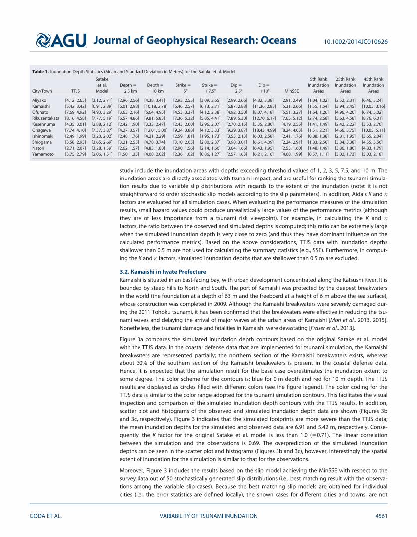
study include the inundation areas with depths exceeding threshold values of 1, 2, 3, 5, 7.5, and 10 m. Theinundation areas are directly associated with tsunami impact, and are useful for ranking the tsunami simula-tion results due to variable slip distributions with regards to the extent of the inundation (note: it is notstraightforward to order stochastic slip models according to the slip parameters). In addition, Aida’s K and jfactors are evaluated for all simulation cases. When evaluating the performance measures of the simulationresults, small hazard values could produce unrealistically large values of the performance metrics (althoughthey are of less importance from a tsunami risk viewpoint). For example, in calculating the K and jfactors, the ratio between the observed and simulated depths is computed; this ratio can be extremely largewhen the simulated inundation depth is very close to zero (and thus they have dominant influence on thecalculated performance metrics). Based on the above considerations, TTJS data with inundation depthsshallower than 0.5 m are not used for calculating the summary statistics (e.g., SSE). Furthermore, in comput-ing the K and j factors, simulated inundation depths that are shallower than 0.5 m are excluded.

3.2. Kamaishi in Iwate PrefectureKamaishi is situated in an East-facing bay, with urban development concentrated along the Katsushi River. It isbounded by steep hills to North and South. The port of Kamaishi was protected by the deepest breakwatersin the world (the foundation at a depth of 63 m and the freeboard at a height of 6 m above the sea surface),whose construction was completed in 2009. Although the Kamaishi breakwaters were severely damaged dur-ing the 2011 Tohoku tsunami, it has been confirmed that the breakwaters were effective in reducing the tsu-nami waves and delaying the arrival of major waves at the urban areas of Kamaishi [Mori et al., 2013, 2015].Nonetheless, the tsunami damage and fatalities in Kamaishi were devastating [Fraser et al., 2013].

Figure 3a compares the simulated inundation depth contours based on the original Satake et al. modelwith the TTJS data. In the coastal defense data that are implemented for tsunami simulation, the Kamaishibreakwaters are represented partially; the northern section of the Kamaishi breakwaters exists, whereasabout 30% of the southern section of the Kamaishi breakwaters is present in the coastal defense data.Hence, it is expected that the simulation result for the base case overestimates the inundation extent tosome degree. The color scheme for the contours is: blue for 0 m depth and red for 10 m depth. The TTJSresults are displayed as circles filled with different colors (see the figure legend). The color coding for theTTJS data is similar to the color range adopted for the tsunami simulation contours. This facilitates the visualinspection and comparison of the simulated inundation depth contours with the TTJS results. In addition,scatter plot and histograms of the observed and simulated inundation depth data are shown (Figures 3band 3c, respectively). Figure 3 indicates that the simulated footprints are more severe than the TTJS data;the mean inundation depths for the simulated and observed data are 6.91 and 5.42 m, respectively. Conse-quently, the K factor for the original Satake et al. model is less than 1.0 (50.71). The linear correlationbetween the simulation and the observations is 0.69. The overprediction of the simulated inundationdepths can be seen in the scatter plot and histograms (Figures 3b and 3c), however, interestingly the spatialextent of inundation for the simulation is similar to that for the observations.

Moreover, Figure 3 includes the results based on the slip model achieving the MinSSE with respect to thesurvey data out of 50 stochastically generated slip distributions (i.e., best matching result with the observa-tions among the variable slip cases). Because the best matching slip models are obtained for individualcities (i.e., the error statistics are defined locally), the shown cases for different cities and towns, are not

Table 1. Inundation Depth Statistics (Mean and Standard Deviation in Meters) for the Satake et al. Model

City/Town TTJS

Satakeet al.

ModelDepth 5

22.5 kmDepth 5

110 kmStrike 5

258

Strike 5

17.58

Dip 5

22.58

Dip 5

1108 MinSSE

5th RankInundation

Areas

25th RankInundation

Areas

45th RankInundation

Areas

Miyako [4.12, 2.65] [3.12, 2.71] [2.96, 2.56] [4.38, 3.41] [2.93, 2.55] [3.09, 2.65] [2.99, 2.66] [4.82, 3.38] [2.91, 2.49] [1.04, 1.02] [2.52, 2.31] [6.46, 3.24]Kamaishi [5.42, 3.42] [6.91, 2.89] [6.01, 2.98] [10.18, 2.78] [6.46, 2.57] [6.13, 2.71] [6.87, 2.88] [11.36, 2.83] [5.31, 2.66] [1.55, 1.54] [3.94, 2.45] [10.05, 3.16]Ofunato [7.69, 4.92] [4.93, 3.29] [3.63, 2.16] [6.64, 4.95] [4.53, 3.37] [4.12, 2.38] [4.92, 3.50] [8.07, 4.18] [5.51, 3.27] [1.64, 1.26] [4.96, 4.20] [6.74, 5.02]Rikuzentakata [8.16, 4.58] [7.77, 5.19] [6.57, 4.86] [9.81, 5.83] [7.36, 5.32] [5.85, 4.41] [7.89, 5.30] [12.70, 6.17] [7.65, 5.12] [2.74, 2.68] [5.63, 4.58] [8.76, 6.01]Kesennuma [4.35, 3.01] [2.88, 2.12] [2.42, 1.90] [3.33, 2.47] [2.43, 2.00] [2.96, 2.07] [2.70, 2.15] [5.35, 2.80] [4.19, 2.55] [1.41, 1.49] [2.42, 2.22] [3.53, 2.70]Onagawa [7.74, 4.10] [7.37, 3.87] [4.27, 3.57] [12.01, 5.00] [9.24, 3.88] [4.12, 3.33] [9.29, 3.87] [18.43, 4.99] [8.24, 4.03] [1.51, 2.21] [4.66, 3.75] [10.05, 5.11]Ishinomaki [2.49, 1.99] [3.20, 2.02] [2.48, 1.76] [4.21, 2.29] [2.59, 1.81] [1.95, 1.73] [3.55, 2.13] [6.03, 2.58] [2.41, 1.76] [0.88, 1.38] [2.81, 1.95] [3.65, 2.04]Shiogama [3.58, 2.93] [3.65, 2.69] [3.21, 2.55] [4.78, 3.74] [3.10, 2.65] [2.80, 2.37] [3.98, 3.01] [6.61, 4.09] [2.24, 2.91] [1.83, 2.50] [3.84, 3.38] [4.55, 3.50]Natori [2.71, 2.07] [3.28, 1.59] [2.62, 1.57] [4.83, 1.88] [2.90, 1.56] [2.14, 1.60] [3.64, 1.66] [6.43, 1.95] [2.53, 1.60] [1.48, 1.49] [3.86, 1.80] [4.83, 1.79]Yamamoto [3.75, 2.79] [2.06, 1.51] [1.50, 1.35] [4.08, 2.02] [2.36, 1.62] [0.86, 1.27] [2.57, 1.63] [6.21, 2.16] [4.08, 1.99] [0.57, 1.11] [3.02, 1.73] [5.03, 2.18]



identical. The MinSSE case is less severe than the original case and achieves closer agreement with the TTJSdata (e.g., mean inundation depth is 5.31 m and the linear correlation is 0.71; see Table 1).

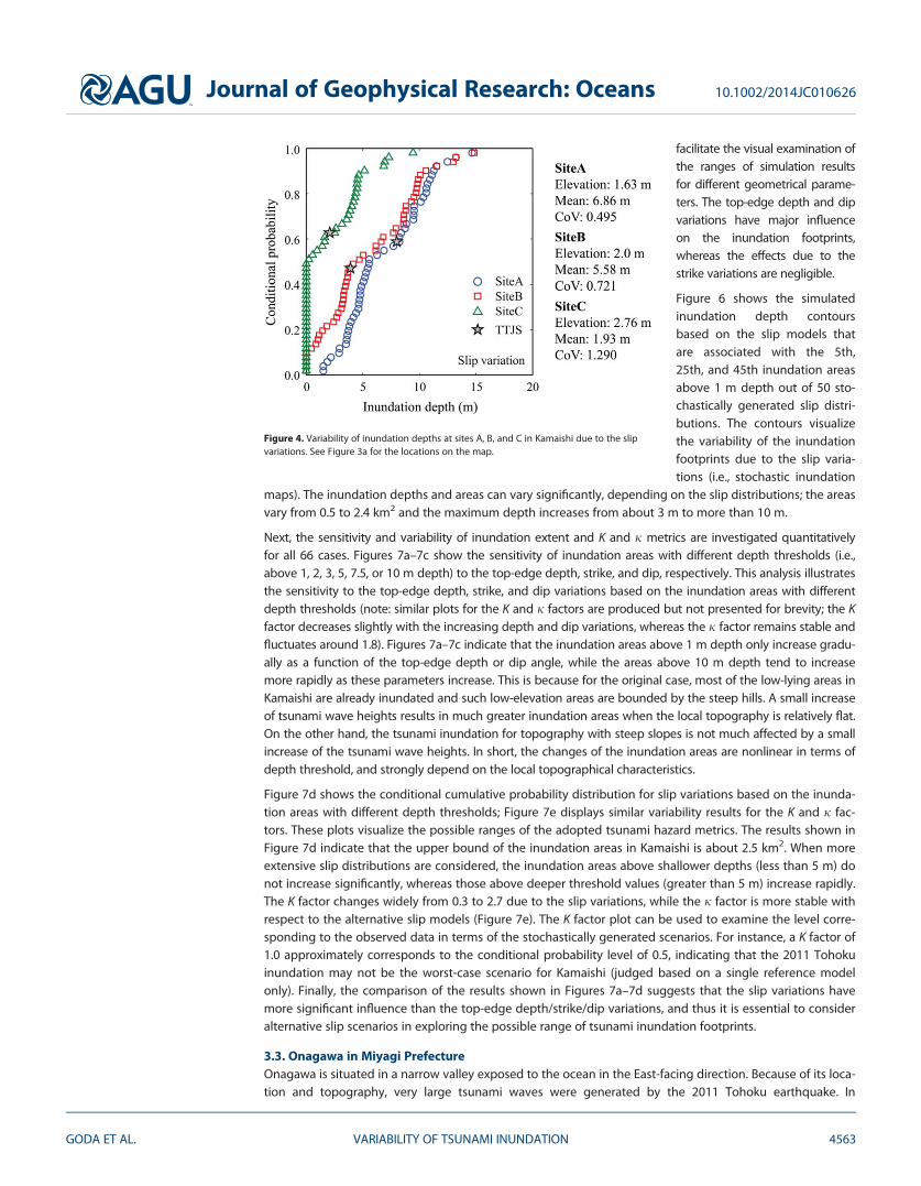
Before discussing tsunami inundation footprints in Kamaishi (which are spatially aggregated tsunami hazardparameters), it is instructive to examine the variability of tsunami inundation depths at specific locationsdue to the slip variations (i.e., 50 cases). For this purpose, the conditional cumulative probability distributionfunctions of the tsunami inundation depths at three TTJS sites are compared in Figure 4. The term condi-tional is included to specify that the tsunami hazard assessments are conducted by referring to a particularscenario (i.e., events similar to the 2011 Tohoku earthquake), rather than all possible events in the Tohokuregion. The locations of the selected TTJS sites are shown in Figure 3a. In the Figure 4 legend, the elevationsas well as the statistics, i.e., mean and coefficient of variation (CoV), of inundation depth for the three sitesare indicated. Additionally, the TTJS observations at the three locations are represented by a star in the fig-ure. For Kamaishi, site A is near the coastline, site B is located in the center of the urban areas, and site C isat further inland (note: the elevations for sites A, B, and C gradually increase; see Figure 3a). As expected,the probability distribution functions of the inundation depth gradually shift toward left as the elevation ofthe TTJS sites becomes higher (this can be inspected by their mean inundation depths). The CoV of theinundation depth tends to become larger as the elevation of the TTJS sites becomes higher. This is becausewhen tsunami sources are distant from Kamaishi (e.g., major asperities are located in the southern/centralpart of the Tohoku region), inland sites are not inundated, while if tsunami sources are close to Kamaishithen massive tsunami waves can inundate the majority of the low-lying part of the city (see Figure 6).

The sensitivity results for variable geometrical parameters are compared in Figure 5, showing simulated inunda-tion depth contours based on the top-edge depth variations of 22.5 km and 110 km, strike variations of 258

and 17.58, and dip variations of 22.58 and 1108 with respect to the reference model (for each parameter, theminimum and maximum cases are presented; see Table 1 for the inundation depth statistics). The contours

Figure 3. Tsunami simulation results for Kamaishi: (a) inundation depth contours, (b) scatter plot, and (c) histograms based on the Satakeet al. model and the minimum SSE slip distribution.



facilitate the visual examination ofthe ranges of simulation resultsfor different geometrical parame-ters. The top-edge depth and dipvariations have major influenceon the inundation footprints,whereas the effects due to thestrike variations are negligible.

Figure 6 shows the simulatedinundation depth contoursbased on the slip models thatare associated with the 5th,25th, and 45th inundation areasabove 1 m depth out of 50 sto-chastically generated slip distri-butions. The contours visualizethe variability of the inundationfootprints due to the slip varia-tions (i.e., stochastic inundation

maps). The inundation depths and areas can vary significantly, depending on the slip distributions; the areasvary from 0.5 to 2.4 km2 and the maximum depth increases from about 3 m to more than 10 m.

Next, the sensitivity and variability of inundation extent and K and j metrics are investigated quantitativelyfor all 66 cases. Figures 7a–7c show the sensitivity of inundation areas with different depth thresholds (i.e.,above 1, 2, 3, 5, 7.5, or 10 m depth) to the top-edge depth, strike, and dip, respectively. This analysis illustratesthe sensitivity to the top-edge depth, strike, and dip variations based on the inundation areas with differentdepth thresholds (note: similar plots for the K and j factors are produced but not presented for brevity; the Kfactor decreases slightly with the increasing depth and dip variations, whereas the j factor remains stable andfluctuates around 1.8). Figures 7a–7c indicate that the inundation areas above 1 m depth only increase gradu-ally as a function of the top-edge depth or dip angle, while the areas above 10 m depth tend to increasemore rapidly as these parameters increase. This is because for the original case, most of the low-lying areas inKamaishi are already inundated and such low-elevation areas are bounded by the steep hills. A small increaseof tsunami wave heights results in much greater inundation areas when the local topography is relatively flat.On the other hand, the tsunami inundation for topography with steep slopes is not much affected by a smallincrease of the tsunami wave heights. In short, the changes of the inundation areas are nonlinear in terms ofdepth threshold, and strongly depend on the local topographical characteristics.

Figure 7d shows the conditional cumulative probability distribution for slip variations based on the inunda-tion areas with different depth thresholds; Figure 7e displays similar variability results for the K and j fac-tors. These plots visualize the possible ranges of the adopted tsunami hazard metrics. The results shown inFigure 7d indicate that the upper bound of the inundation areas in Kamaishi is about 2.5 km2. When moreextensive slip distributions are considered, the inundation areas above shallower depths (less than 5 m) donot increase significantly, whereas those above deeper threshold values (greater than 5 m) increase rapidly.The K factor changes widely from 0.3 to 2.7 due to the slip variations, while the j factor is more stable withrespect to the alternative slip models (Figure 7e). The K factor plot can be used to examine the level corre-sponding to the observed data in terms of the stochastically generated scenarios. For instance, a K factor of1.0 approximately corresponds to the conditional probability level of 0.5, indicating that the 2011 Tohokuinundation may not be the worst-case scenario for Kamaishi (judged based on a single reference modelonly). Finally, the comparison of the results shown in Figures 7a–7d suggests that the slip variations havemore significant influence than the top-edge depth/strike/dip variations, and thus it is essential to consideralternative slip scenarios in exploring the possible range of tsunami inundation footprints.

3.3. Onagawa in Miyagi PrefectureOnagawa is situated in a narrow valley exposed to the ocean in the East-facing direction. Because of its loca-tion and topography, very large tsunami waves were generated by the 2011 Tohoku earthquake. In

Figure 4. Variability of inundation depths at sites A, B, and C in Kamaishi due to the slipvariations. See Figure 3a for the locations on the map.



particular, the majority of buildings in low-lying areas were completely inundated and destroyed; the maxi-mum inundation depths exceeded 16 m. In addition to the direct tsunami effects, a large subsidence of1.2 m was observed in Onagawa due to coseismic deformation of the 2011 Tohoku earthquake. Because ofthe very large tsunami waves arriving within a relatively short time after the earthquake (about 30 min), thefatality rate among the population residing in the inundated areas was particularly high in Onagawa [Fraseret al., 2013].

The same set of tsunami simulation results that are considered for Kamaishi (i.e., Figures 3–7) is presented inFigures 8–12 for Onagawa. The inundated areas based on the Satake et al. model are in good agreement with

Figure 5. Sensitivity of inundation depth contours for Kamaishi: (a) top-edge depths of 22.5 km and 110 km, (b) strike angles of 258 and 17.58, and (c) dip angles of 22.58 and 1108.



the observed inundation data (Figure 8a). The very deep inundation at the low-lying parts of Onagawa can beobserved clearly. Although the number of the TTJS data points is relatively small, the scatter plot and histo-grams of the simulated and observed data show good agreement (e.g., mean inundation depths of 7.37 ver-sus 7.74 m; K factor 5 0.98; Figures 8b and 8c). The linear correlation coefficient is 0.81. Furthermore, theinundation depth contours for the MinSSE case is similar to (but slightly more severe than) the original case.

Figure 9 compares the conditional cumulative probability distribution functions of inundation depths atthree TTJS locations (see Figure 8a) in Onagawa due to the slip variations. The results show that the variabil-ity of tsunami inundation depths at specific sites can be large. The average inundation depth decreaseswith the distance from the coastline (i.e., elevation of the sites increases), whereas the CoV of inundationdepth increases.

The sensitivity analysis for the geometrical parameters shows that all three parameters have significantinfluence on the tsunami inundation (Figure 10). Inundation depth increases with the top-edge depth anddip variations, while it decreases with the strike variations (Figures 12a–12c). The strong sensitivity to thefault strike is attributed to the fact that Onagawa directly faces major earthquake rupture areas of the 2011

Figure 6. Inundation depth contours for Kamaishi: 5th rank, 25th rank, and 45th rank based on the inundation areas above 1 m depth out of 50 stochastic slip cases.

Figure 7. Sensitivity analysis results for Kamaishi: sensitivity of inundation areas to the (a) top-edge depth variations, (b) strike variations, (c) dip variations, (d) variability of inundationareas, and (e) K and j factors due to the slip variations.



Tohoku earthquake (see Figure2). The high sensitivity to thegeometrical parameters is alsoobserved for the K factor, whilethe j factor slightly varies withthe top-edge depth and strikevariations, but remains almostconstant for the dip variations(note: results are omitted forbrevity).

The ranked inundation footprintsbased on the inundation areasabove 1 m depth (Figure 11) sug-gest that the spatial extent of theinundated areas changes fromthe 5th rank case to the 25thrank case. On the other hand,from the 25th rank case to the45th rank case, major changes

Figure 8. Tsunami simulation results for Onagawa: (a) inundation depth contours, (b) scatter plot, and (c) histograms based on the Satakeet al. model and the minimum SSE slip distribution.

Figure 9. Variability of inundation depths at sites A, B, and C in Onagawa due to the slipvariations. See Figure 8a for the locations on the map.



occur mostly to inundation depths, rather than inundation areas. Such trends can also be seen in Figure 12d;the inundation areas for all depth thresholds are practically bounded at 1 km2. Figure 12e shows that the Kfactor varies very widely (from 0.5 to 5.0) due to the slip variations, indicating that the tsunami inundation in

Figure 10. Sensitivity of inundation depth contours for Onagawa: (a) top-edge depths of 22.5 km and 110 km, (b) strike angles of 258

and 17.58, and (c) dip angles of 22.58 and 1108.



Onagawa is very sensitive to slip characteristics. The conditional probability level corresponding to the K factorof 1.0 is 0.2; thus the observed tsunami during the 2011 Tohoku event may be considered as one of theworst-case scenarios for this town.

3.4. Sendai-Natori-Iwanuma in Miyagi PrefectureSendai, Natori, and Iwanuma are positioned in the Sendai plain (note: the Sendai airport is inIwanuma). They are the most populated areas in Miyagi Prefecture. Two major rivers, the Natori Riverand the Abukuma River, run through the areas. The flat terrain contributed significantly to extensiveinundation areas during the 2011 Tohoku tsunami. The inundation reached the Sendai Tobu Highway,which runs South-North at about 2–5 km from the coast. The 10 m embankment of the highwayreduced the tsunami inundation significantly [Goto et al., 2012]. The destruction of residential districtsnear the shoreline (e.g., Arahama and Yuriage) was particularly severe. Because of the unexpectedly

Figure 11. Inundation depth contours for Onagawa: 5th rank, 25th rank, and 45th rank based on the inundation areas above 1 m depth out of 50 stochastic slip cases.

Figure 12. Sensitivity analysis results for Onagawa: sensitivity of inundation areas to the (a) top-edge depth variations, (b) strike variations, (c) dip variations, (d) variability of inundationareas, and (e) K and j factors due to the slip variations.



large tsunami, the fatality rates in the severely inundated areas were relatively high [Fraser et al.,2013].

The same set of tsunami simulation results that are considered for Kamaishi (i.e., Figures 3–7) is pre-sented in Figures 13–17 for Sendai-Natori-Iwanuma. Figure 13 compares the inundated areas based onthe Satake et al. model and the TTJS data. Generally, the simulated and observed data are in agreement;the mean inundation depths of the simulated and observed data are 3.28 and 2.71 m, respectively (Kfactor 5 0.70), and the linear correlation coefficient is 0.69. In the tsunami simulations, the embankmentof the highway is not represented in the DEM, and thus the spatial extent of the simulated inundationto further inland may be overestimated. Another notable feature of the tsunami inundation contours inSendai is the narrow strip of land that has particularly large inundation depths along the shoreline. Thiscorresponds to a segment of Teizan Canal, which connects Shiogama and Iwanuma. Moreover, the

inundation depth contours forthe MinSSE case are similar, butslightly more severe than theoriginal case.

Figure 15 shows the variability ofinundation depths at three TTJSlocations in Natori due to the slipvariations. Because of the flat ter-rain in Sendai plain, the eleva-tions of the three TTJS sites aresimilar but the distances fromthe shoreline are different (Fig-ure 14a). The conditional cumula-tive probability distribution plotsof the inundation depths at thethree locations clearly show thatthe average inundation depthdecreases with the distance from

Figure 13. Tsunami simulation results for Sendai-Natori-Iwanuma: (a) inundation depth contours, (b) scatter plot, and (c) histograms based on the Satake et al. model and the minimumSSE slip distribution.

Figure 14. Variability of inundation depths at sites A, B, and C in Sendai-Natori-Iwanumadue to the slip variations. See Figure 13a for the locations on the map.



the shoreline. This is due to the bottom friction. Further to note, the CoV values for the TTJS sites in Natoriare significantly smaller than those in Kamaishi and Onagawa. The result is influenced by the location andextent of major asperities and the topographical features [see also Goda et al., 2014].

The sensitivity analysis for the geometrical parameters (Figure 15) indicates that the top-edge depth anddip parameters have major influence on the tsunami inundation, while the effects due to the strike varia-tions are less pronounced. The inundation areas for shallow and deep depth thresholds exhibit differenttendencies (Figures 17a–17c). The inundation areas for depths less than 5 m are affected by variations ofgeometrical parameters. On the other hand, the inundation areas for depth greater than 5 m are less sensi-tive to such changes. These trends are due to the flat terrain of this region. Variations in geometrical param-eters have only moderate influence on the K factor.

The ranked inundation footprints based on the inundation areas above 1 m depth (Figure 16) suggest thatboth spatial inundation extent and inundation depth increase as the considered scenario becomes moreextreme. For the worst-case scenario, the inundation areas above 1 m depth reach a topographical boundarywhere the elevations start to become steeper. This tendency can be seen in the conditional cumulative proba-bility distribution function plot of the inundation depths (Figure 17d); the curve for the 1 m depth threshold

Figure 15. Sensitivity of inundation depth contours for Sendai-Natori-Iwanuma: (a) top-edge depths of 22.5 km and 110 km, (b) strike angles of 258 and 17.58, and (c) dip angles of22.58 and 1108.



initially increases gradually, but the slope of the curve becomes steeper (nearly vertical) as the conditionalprobability level increases. The K factor for slip variations (Figure 17e) exhibits a unique feature; for the major-ity of the slip cases (up to the conditional probability level of 0.8), the K factor varies within a narrow rangebetween 0.4 and 1.0, while only a small subset of the cases has the K factor greater than 1.0. This indicates

Figure 16. Inundation depth contours for Sendai-Natori-Iwanuma: 5th rank, 25th rank, and 45th rank based on the inundation areas above 1 m depth out of 50 stochastic slip cases.

Figure 17. Sensitivity analysis results for Sendai-Natori-Iwanuma: sensitivity of inundation areas to the (a) top-edge depth variations, (b) strike variations, and (c) dip variations, and (d)variability of inundation areas and (e) K and j factors due to the slip variations.



that the chance of experiencing a similar tsunami inundation extent as for the 2011 Tohoku earthquake maybe considered likely in a future Mw9 subduction earthquake in the Tohoku region.

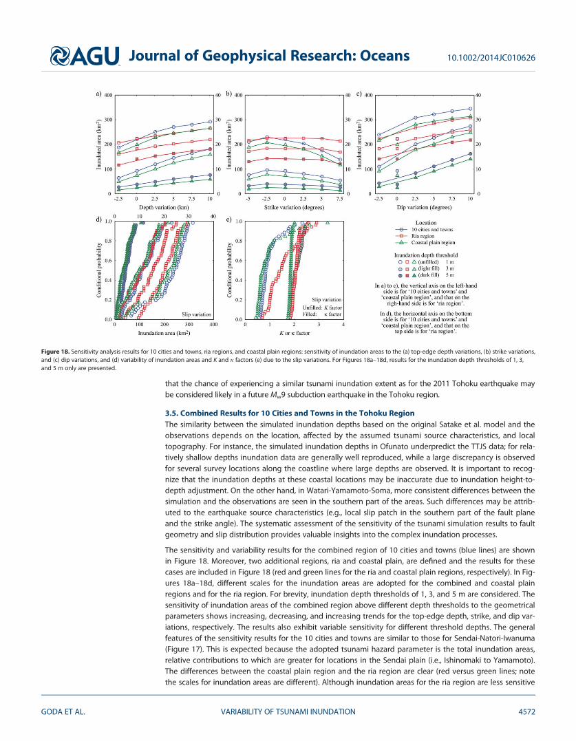
3.5. Combined Results for 10 Cities and Towns in the Tohoku RegionThe similarity between the simulated inundation depths based on the original Satake et al. model and theobservations depends on the location, affected by the assumed tsunami source characteristics, and localtopography. For instance, the simulated inundation depths in Ofunato underpredict the TTJS data; for rela-tively shallow depths inundation data are generally well reproduced, while a large discrepancy is observedfor several survey locations along the coastline where large depths are observed. It is important to recog-nize that the inundation depths at these coastal locations may be inaccurate due to inundation height-to-depth adjustment. On the other hand, in Watari-Yamamoto-Soma, more consistent differences between thesimulation and the observations are seen in the southern part of the areas. Such differences may be attrib-uted to the earthquake source characteristics (e.g., local slip patch in the southern part of the fault planeand the strike angle). The systematic assessment of the sensitivity of the tsunami simulation results to faultgeometry and slip distribution provides valuable insights into the complex inundation processes.

The sensitivity and variability results for the combined region of 10 cities and towns (blue lines) are shownin Figure 18. Moreover, two additional regions, ria and coastal plain, are defined and the results for thesecases are included in Figure 18 (red and green lines for the ria and coastal plain regions, respectively). In Fig-ures 18a–18d, different scales for the inundation areas are adopted for the combined and coastal plainregions and for the ria region. For brevity, inundation depth thresholds of 1, 3, and 5 m are considered. Thesensitivity of inundation areas of the combined region above different depth thresholds to the geometricalparameters shows increasing, decreasing, and increasing trends for the top-edge depth, strike, and dip var-iations, respectively. The results also exhibit variable sensitivity for different threshold depths. The generalfeatures of the sensitivity results for the 10 cities and towns are similar to those for Sendai-Natori-Iwanuma(Figure 17). This is expected because the adopted tsunami hazard parameter is the total inundation areas,relative contributions to which are greater for locations in the Sendai plain (i.e., Ishinomaki to Yamamoto).The differences between the coastal plain region and the ria region are clear (red versus green lines; notethe scales for inundation areas are different). Although inundation areas for the ria region are less sensitive

Figure 18. Sensitivity analysis results for 10 cities and towns, ria regions, and coastal plain regions: sensitivity of inundation areas to the (a) top-edge depth variations, (b) strike variations,and (c) dip variations, and (d) variability of inundation areas and K and j factors (e) due to the slip variations. For Figures 18a–18d, results for the inundation depth thresholds of 1, 3,and 5 m only are presented.



to increase in top-edge depth variation, inundation areas for the coastal plain region increase monotonicallyas the depth variation increases. The depth variation gives a factor of 2–3 difference for inundation areas inthe coastal plain region. The positive strike variation decreases the inundation areas in the coastal plainregion, but gives less influence in the ria coast region (at more local levels, the strike variation does affectinundation areas, e.g., Onagawa; see Figure 12b). Generally, the sensitivity of tsunami inundation areas tofault geometry is significant in the coastal plain region. Therefore, it is important to know how sensitive atarget region is to fault geometry for expected tsunami scenarios.

It is noteworthy that the impacts of the fault geometry and slip distribution vary spatially along the Tohokucoast (i.e., ria region to coastal plain region), indicating that critical scenarios with similar magnitudes fortsunami hazard mapping and planning should be developed by taking into account such key features.

4. Conclusions

This study investigated the sensitivity and variability of tsunami inundation footprints in 10 coastal citiesand towns due to a megathrust subduction earthquake in the Tohoku region of Japan by considering differ-ent fault geometry and slip distributions. The variations of earthquake source characteristics were repre-sented with respect to the Satake et al. source model by changing the top-edge depth, strike, dip, and slipdistributions. The slip variations were implemented based on the spectral analysis and synthesis method fora Mw9 megathrust subduction earthquake, developed by Goda et al. [2014]. For evaluating inundation foot-prints at submunicipality levels, tsunami simulations were carried out using bathymetry and elevation datawith 50 m grid spatial resolution. The investigations facilitated the development of stochastic inundationdepth maps and the variability assessment of tsunami hazard estimates. Such information is critical toanticipate the potential consequences under different conditions, and to communicate variability associ-ated with hazard predictions for tsunami risk management purposes.

The main conclusions of this study are:

1. The sensitivity of inundation areas and performance metrics (e.g., K and j factors) to the geometricalparameters is nontrivial. An increase in top-edge depth results in greater tsunami inundation. In particu-lar, when large slip exists at shallow depth near the Trench, the impact of the depth variations tend to begreater. The effects due to the strike variations can be either constant, increasing, decreasing, or combi-nation of those, and depend on the location of large slip asperities relative to the site location. Anincrease in dip leads to greater tsunami inundation.

2. The variability of inundation footprints due to variable slip distributions can be significant. Generallyspeaking, the effects due to the slip variations are more significant than those due to the variable geo-metrical parameters of the earthquake source. Using stochastically generated earthquake slip models,many realizations of inundation depth maps can be obtained. These are particularly effective in visualiz-ing and communicating uncertainty associated with the tsunami input boundary conditions. These inun-dation simulations are also useful for evaluating observed (historical) tsunami inundation cases in termsof the possible ranges of the inundation depths and areas for future scenarios.

3. Both the sensitivity and variability assessments of tsunami inundation depths depend strongly on localtopography. In ria regions, where cities and towns are surrounded by steep hills, the spatial extent of tsu-nami inundation is often determined by the abrupt changes of elevation. In such cases, the inundationareas for different depth thresholds are not significantly affected but their depths increase greatly. Onthe other hand, in coastal plain regions, tsunami inundation areas vary significantly for different tsunamiscenarios. Therefore, it is of critical importance to account for nonlinear inundation processes and topo-graphical effects when assessing uncertainty in developing tsunami hazard maps, but also for generatingevacuation maps for local communities.

ReferencesAida, I. (1978), Reliability of tsunami source model derived from fault parameters, J. Phys. Earth, 26, 57–73.Bilek, S. L., and T. Lay (1999), Rigidity variations with depth along interpolate mega-thrust faults in subduction zones, Nature, 400, 443–446.Federal Emergency Management Agency (FEMA) (2008), Guidelines for design of structures for vertical evacuation from tsunamis, FEMA

P646, Fed. Emergency Manage. Agency, Washington, D. C.

AcknowledgmentsThe bathymetry and elevation data forthe Tohoku region were providedby the Cabinet Office of the JapaneseGovernment. The runup andinundation survey data were obtainedfrom the 2011 Tohoku EarthquakeTsunami Joint Survey Group (http://www.coastal.jp/tsunami2011/). Thiswork was supported by theEngineering and Physical SciencesResearch Council (EP/M001067/1) aswell as by the King Abdullah Universityof Science and Technology (KAUST).The authors thank two anonymousreviewers for their insightfulcomments and suggestions thatimproved the clarity of the papersignificantly.



http://www.coastal.jp/tsunami2011/

http://www.coastal.jp/tsunami2011/

Fraser, S., A. Pomonis, A. Raby, K. Goda, S. C. Chian, J. Macabuag, M. Offord, K. Saito, and P. Sammonds (2013), Tsunami damage to coastaldefences and buildings in the March 11th 2011 Mw9.0 Great East Japan earthquake and tsunami, Bull. Earthquake Eng., 11, 205–239.

Fujii, Y., K. Satake, S. Sakai, S. Shinohara, and T. Kanazawa (2011), Tsunami source of the 2011 off the Pacific coast of Tohoku earthquake,Earth Planets Space, 63, 815–820.

Geist, E. L. (2002), Complex earthquake rupture and local tsunamis, J. Geophys. Res., 107(B5), 2086, doi:10.1029/2000JB000139.Geist, E. L., and S. L. Bilek (2001), Effect of depth-dependent shear modulus on tsunami generation along subduction zones, Geophys. Res.

Lett., 28, 1315–1318, doi:10.1029/2000GL012385.Geist, E. L., and T. Parsons (2006), Probabilistic analysis of tsunami hazards, Nat. Hazards, 37, 277–314.Glimsdal, S., G. K. Pedersen, C. B. Harbitz, and F. Løvholt (2013), Dispersion of tsunamis: Does it really matter?, Nat. Hazards Earth Syst. Sci.,

13, 1507–1526.Goda, K., P. M. Mai, T. Yasuda, and N. Mori (2014), Sensitivity of tsunami wave profiles and inundation simulations to earthquake slip and

fault geometry for the 2011 Tohoku earthquake, Earth Planets Space, 66, 105, doi:10.1186/1880–5981-66–105.Goto, C., Y. Ogawa, N. Shuto, and F. Imamura (1997), Numerical method of tsunami simulation with the leap-frog scheme (IUGG/IOC Time

Project), IOC Manual 35, The United Nations Educational, Scientific and Cultural Organization, (UNESCO) Paris.Goto, K., K. Fujima, D. Sugawara, S. Fujino, K. Imai, R. Tsudaka, T. Abe, and T. Haraguchi (2012), Field measurements and numerical

modeling for the run-up heights and inundation distances of the 2011 Tohoku-oki tsunami at Sendai Plain, Japan, Earth Planets Space,64, 1247–1257.

Gusman, A. R., Y. Tanioka, S. Sakai, and H. Tsushima (2012), Source model of the great 2011 Tohoku earthquake estimated from tsunamiwaveforms and crustal deformation data, Earth Planet. Sci. Lett., 341–344, 234–242.

Hooper, A., J. Pietrzak, W. Simons, H. Cui, R. Riva, M. Naeije, A. Terwisscha van Scheltinga, E. Schrama, G. Stelling, and A. Socuet (2013),Importance of horizontal seafloor motion on tsunami height for the 2011 Mw 5 9.0 Tohoku-Oki earthquake, Earth Planet. Sci. Lett., 261,469–479.

Horspool, N., I. Pranantyo, J. Griffin, H. Latief, D. H. Natawidjaja, W. Kongko, A. Cipta, B. Bustaman, S. D. Anugrah, and H. K. Thio (2014), Aprobabilistic tsunami hazard assessment for Indonesia, Nat. Hazards Earth Syst. Sci., 14, 3105–3122.

Ichihara, H., Y. Hamano, K. Baba, and T. Kasaya (2013), Tsunami source of the 2011 Tohoku earthquake detected by an ocean-bottom mag-netometer, Earth Planet. Sci. Lett., 382, 117–124.

Iwasaki, T., and A. Mano (1979), Numerical simulation of two-dimensional tsunami run up by Euler’s coordinates, in Proceedings of the 26thJapanese Conference on Coastal Engineering [in Japanese], pp. 70–74.

Japan Society of Civil Engineers (JSCE) (2002), Tsunami assessment method for nuclear power plants in Japan, Tokyo, Japan. [Available athttp://committees.jsce.or.jp/ceofnp/node/5.]

Kagan, Y., and D. D. Jackson (2013), Tohoku earthquake: A surprise?, Bull. Seismol. Soc. Am., 103, 1181–1194.Kaiser, G., L. Scheele, A. Kortenhaus, F. Løvholt, H. R€omer, and S. Leschka (2011), The influence of land cover roughness on the results of

high resolution tsunami inundation modeling, Nat. Hazards Earth Syst. Sci., 11, 2521–2540.Kajiura, K. (1963), The leading wave of a tsunami, Bull. Earthquake Res. Inst., 41, 535–571.Koshimura, S., T. Oie, H. Yanagisawa, and F. Imamura (2009), Developing fragility functions for tsunami damage estimation using numerical

model and post-tsunami data from Banda Aceh, Indonesia, Coastal Eng. J., 51, 243–273.Lavall�ee, D., P. Liu, and R. J. Archuleta (2006), Stochastic model of heterogeneity in earthquake slip spatial distributions, Geophys. J. Int.,

165, 622–640.Løvholt, F., G. Pedersen, S. Bazin, D. Kuhn, R. E. Bredesen, and C. Harbitz (2012), Stochastic analysis of tsunami runup due to heterogeneous

coseismic slip and dispersion, J. Geophys. Res., 117, C03047, doi:10.1029/2011JC007616.MacInnes, B. T., A. R. Gusman, R. J. Le Veque, and Y. Tanioka (2013), Comparison of earthquake source models for the 2011 Tohoku event

using tsunami simulations and near-field observations, Bull. Seismol. Soc. Am., 103, 1256–1274.Mai, P. M., and G. C. Beroza (2002), A spatial random field model to characterize complexity in earthquake slip, J. Geophys. Res., 107(B11),

2308, doi:10.1029/2001JB000588.Mai, P. M., and K. K. S. Thingbaijam (2014), SRCMOD: An online database of finite-fault rupture model, Seismol. Res. Lett., 85, 1348–1357.Mai, P. M., P. Spudich, and J. Boatwright (2005), Hypocenter locations in finite-source rupture models, Bull. Seismol. Soc. Am., 95, 965–980.McCloskey, J., A. Antonioli, A. Piatanesi, K. Sieh, S. Steacy, S. Nalbant, M. Cocco, C. Giunchi, J. D. Huang, and P. Dunlop (2008), Tsunami

threat in the Indian Ocean from a future megathrust earthquake west of Sumatra, Earth Planet. Sci. Lett., 265, 61–81.Mori, N., and T. Takahashi (2012), The 2011 Tohoku Earthquake Tsunami Joint Survey Group, 2012. Nationwide post event survey and

analysis of the 2011 Tohoku earthquake tsunami, Coastal Eng. J., 54, 1250001-1-27.Mori, N., T. Takahashi, T. Yasuda, and H. Yanagisawa (2011), Survey of 2011 Tohoku earthquake tsunami inundation and run-up, Geophys.

Res. Lett., 38, L00G14, doi:10.1029/2011GL049210.Mori, N., D. T. Cox, T. Yasuda, and H. Mase (2013), Overview of the 2011 Tohoku earthquake tsunami damage and its relation to coastal

protection along the Sanriku coast, Earthquake Spectra, 29, S127–S143.Mori, N., N. Yoneyama, and W. Pringle (2015), Effects of the offshore barrier against the 2011 off the Pacific coast of Tohoku earthquake

tsunami and lessons learned, in Post Tsunami Hazards: Restoration and Reconstruction, edited by V. Santiago-Fandino, Y. A. Kontar, andY. Kaneda, pp. 121–132, Springer International Publishing, Springer, Switzerland, doi:10.1007/978-3-319-10202-3_9.

Murata, S., F. Imamura, K. Katoh, Y. Kawata, S. Takahashi, and T. Takayama (2010), Tsunami: To Survive From Tsunami, 316 pp., World Sci.,Hackensack, N. J.

Murotani, S., K. Satake, and Y. Fujii (2013), Scaling relations of seismic moment, rupture area, average slip, and asperity size for M�9subduction-zone earthquakes, Geophys. Res. Lett., 40, 5070–5074, doi:10.1002/grl.50976.

Okada, Y. (1985), Surface deformation due to shear and tensile faults in a half-space, Bull. Seismol. Soc. Am., 75, 1135–1154.Pang, A. (2008), Visualizing uncertainty in natural hazards, Risk Gov. Soc., 14, 261–294.Pardo-Iguzquiza, E., and M. Chica-Olmo (1993), The Fourier integral method: An efficient spectral method for simulation of random fields,

Math. Geol., 25, 177–217.Razafindrakoto, H. N. T., P. M. Mai, M. G. Genton, L. Zhang, and K. K. S. Thingbaijam (2015), Quantifying variability in earthquake rupture

models using multidimensional scaling: Application to the 2011 Tohoku earthquake, Geophys. J. Int., 202, 17–40.Reese, S., B. A. Bradley, J. Bind, G. Smart, W. Power, and J. Sturman (2011), Empirical building fragilities from observed damage in the 2009

South Pacific tsunami, Earth Sci. Rev., 107, 156–173.Satake, K., Y. Fujii, T. Harada, and Y. Namegaya (2013), Time and space distribution of coseismic slip of the 2011 Tohoku earthquake as

inferred from tsunami waveform data, Bull. Seismol. Soc. Am., 103, 1473–1492.Shuto, N. (1991), Numerical simulation of tsunamis—Its present and near future, Nat. Hazards, 4, 171–191.



http://dx.doi.org/10.1029/2000JB000139

http://dx.doi.org/10.1029/2000GL012385

http://dx.doi.org/10.1186/1880-5981-66-105

http://committees.jsce.or.jp/ceofnp/node/5

http://dx.doi.org/10.1029/2011JC007616

http://dx.doi.org/10.1029/2001JB000588

http://dx.doi.org/10.1029/2011GL049210

http://dx.doi.org/10.1007/978-3-319-10202-3_9.

http://dx.doi.org/10.1002/grl.50976

Somerville, P. G., K. Irikura, R. Graves, S. Sawada, D. J. Wald, N. A. Abrahamson, Y. Iwasaki, T. Kagawa, N. Smith, and A. Kowada (1999),Characterizing crustal earthquake slip models for the prediction of strong ground motion, Seismol. Res. Lett., 70, 59–80.

Suppasri, A., E. Mas, I. Charvet, R. Gunasekera, K. Imai, Y. Fukutani, Y. Abe, and F. Imamura (2013), Building damage characteristics based onsurveyed data and fragility curves of the 2011 Great East Japan tsunami, Nat. Hazards, 66, 319–341.

Tanioka, Y., and K. Satake (1996), Tsunami generation by horizontal displacement of ocean bottom, Geophys. Res. Lett., 23, 861–864.Tappin, D. R., S. T. Grilli, J. C. Harris, R. J. Geller, T. Masterlark, J. T. Kirby, F. Shi, G. Ma, K. K. S. Thingbaijam, and P. M. Mai (2014), Did a

submarine landslide contribute to the 2011 Tohoku tsunami?, Mar. Geol., 357, 344–361.Thio, H. K., P. Somerville, and G. Ichihara (2007), Probabilistic analysis of strong ground motion and tsunami hazards in southeast Asia,

J. Earthquake Tsunami, 1, 119–137.Yamazaki, Y., T. Lay, K. F. Cheung, H. Yue, and H. Kanamori (2011), Modeling near-field tsunami observations to improve finite-fault slip

models for the 11 March 2011 Tohoku earthquake, Geophys. Res. Lett., 38, L00G15, doi:10.1029/2011GL049130.



http://dx.doi.org/10.1029/2011GL049130

variability of tsunami inundation footprints considering ... fileresearch article...

Documents