variable elimination and conditioning: complexity forecasts

1

CS3710 Advanced Topics in AI, Lecture 6

Variable Elimination and Conditioning: Complexity Forecasts.

Collin [email protected]

Milos [email protected]

9/19/2005

Outline

Recap. Factor-Based Elimination. Moral Graphs and Triangulation. Variable Elimination. Induced Graph. Correspondence with Tree Decomposition. Initial Conclusions. Conditioning. Final Conclusions.

2

Recap (Problem).

Coherence

Difficulty Intelligence

Grade SAT

Letter

Job

Happy

Recap (Variable Elimination)

)(

),(

),,(),,(

),(),(),(),,(...

)(),,(),,(),(),(),,()(

),()(),,(),,(),(),(),,()(

),,(),,(),(),(),,(),()()()(

,

,

,,,,,

,,,,,

,,,,,,

j

jl

jslslj

jggsglslj

cjghsljglisdigi

cdcjghsljglisdigi

jghsljglisdigcdicJp

I

IS

GIS

DIHGSL

CDIHGSL

CDIHGSL

τ

τ

τφ

ττφφ

τφφφφφφ

φφφφφφφφ

φφφφφφφφ

=

=

=

=

=

=

=

∑

∑

∑∑

∑

∑∑

∑

Coherence

Difficulty

Intelligence

Grade SAT

Letter

Job

Happy

3

Basic messages

Variable Elimination is not determininistic. The order of elimination governs the overall

efficiency. Finding an optimal ordering is difficult. While different methodologies exist they are all

functionally identical. The cost of any ordering is exponential in the

number of variables that appear in the largest factor.

Factor-Based Elimination.

)(

),(

),,(),,(

),(),(),(),,(...

)(),,(),,(),(),(),,()(

),()(),,(),,(),(),(),,()(

),,(),,(),(),(),,(),()()()(

,

,

,,,,,

,,,,,

,,,,,,

j

jl

jslslj

jggsglslj

cjghsljglisdigi

cdcjghsljglisdigi

jghsljglisdigcdicJp

I

IS

GIS

DIHGSL

CDIHGSL

CDIHGSL

τ

τ

τφ

ττφφ

τφφφφφφ

φφφφφφφφ

φφφφφφφφ

=

=

=

=

=

=

=

∑

∑

∑∑

∑

∑∑

∑

4

FBE: Trace

FBE: Trace

2L7

3S6

4G5

3H4

3I3

3D2

2C1

ComplexityNew FactorFactors UsedVarStep

),(),,(),,(

),(),(),(),,(

),(),()()(),,(

),()(

6

5

34

2

1

LJSLJSLJ

GLSGJGJGH

IGISIDDIG

CDC

J

L

H

SI

G

DC

τφτ

φττφ

τφφτφ

φφ

)(),(),,(

),(),(),(

)(

7

6

5

4

3

2

1

JLJSLJ

JGSGIG

D

τττττττ

5

Factor-based elimination Ordering Ω:

– A permutation of variables for elimination.

Factor Φ(X,Y) ℜ:– A function mapping some set of variables to a real

value.

scope[Φ]: – The set of variables represented in the factor.

width[Ω] : – The scope of the largest factor produced by Ω.

FBE: Steps

• FBE consists of a series of elimination steps.

• Each step is as follows:– Select a variable X from the set of variables remaining.– Multiply all factors τ where X ∈scope[τ] to produce a

new factor ψ. – Sum X out of ψ to produce a new factor τ whose scope is ψ minus X.

• Repeat until a single factor τ(Y) remains where Y is the target variable of our inference.

6

Complexity

• The complexity of each elimination step is:– Where:

• The complexity of the algorithm for a given ordering Ω is:– Where:

• n is the initial number of factors in the graph.• .

|)(|

...1

ii

ki

scopeNi

ψ

φφψ

=

××=

)( iikNO

][max Ω= widthN

)( maxnNO

FBE: Trace

7

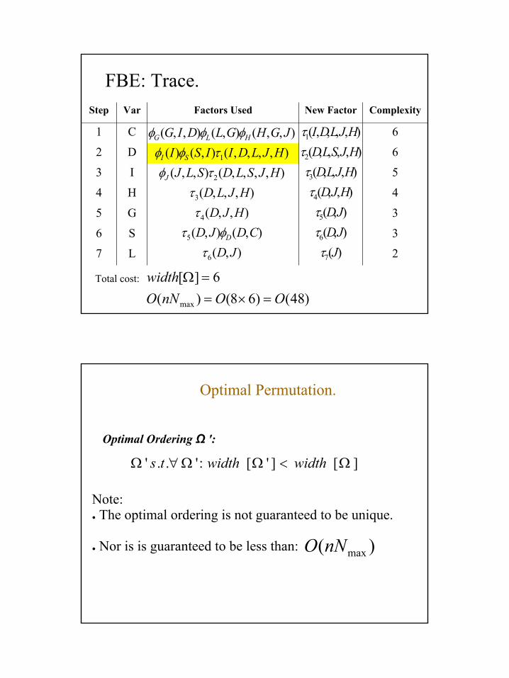
FBE: Trace.

2L73S64G53H43I33D22C1


),(),,(),,(

),(),(),(),,(

),(),()()(),,(

),()(

6

5

34

2

1

LJSLJSLJ

GLSGJGJGH

IGISIDDIG

CDC

J

L

H

SI

G

DC

τφτ

φττφ

τφφτφ

φφ

)(),(

),,(),(),(),(

)(

7

6

5

4

3

2

1

JLJ

SLJJGSGIG

D

ττ

τττττ

Total cost:

)32()48()(4][

max OOnNOwidth

=×==Ω

Ordering 2

8

FBE: Trace.

2L7

3S6

3G5

4H4

5I3

6D2

6C1


),(),(),(

),,(),,,(

),,,,(),,(),,,,(),()(),,(),(),,(

6

5

4

3

2

1

JDCDJD

HJDHJLD

HJSLDSLJHJLDIISI

JGHGLDIG

D

J

SI

HLG

τφτ

ττ

τφτφφ

φφφ

)(),(),(),,(),,,(),,,,(),,,,(

7

6

5

4

3

2

1

JJDJDHJDHJLDHJSLDHJLDI

τττττττ

Total cost:

)48()68()(6][

max OOnNOwidth

=×==Ω

Optimal Permutation.

Optimal Ordering Ω ':

Note: The optimal ordering is not guaranteed to be unique.

Nor is is guaranteed to be less than:

][]'[:'..' Ω<ΩΩ∀Ω widthwidthts

)( maxnNO

9

Moral Graphs

Moral-graph H[G]: of a bayesian network over X is an undirected graph over X that contains an edge between x and y if:

There exists a directed edge between them in G.

They are both parents of the same node in G.

C

D I

G S

L

JH

C

D I

G S

L

JH

Moral Graphs

Why moralization?

),,(),,(),(),(),,(),()(),|(),|()|()|(),|()|()(

),,,,,,,(

7654321 JGHSLJGLISDIGCDCJGHPSLJPGLPISPDIGPCDPCP

HJLSIGDCP

φφφφφφφ==

=

),|( DIGP ),,(3 DIGφC

D I

G S

L

JH

C

D I

G S

L

JH

10

Variable Elimination

The variable elimination algorithm is based only on the scope of each factor.

Factors are distilled from the graph representation.

Variable Elimination can therefore be viewed as a graph algorithm.

C

D I

G S

L

JH

VE: Trace (1)

(1)

∑=C

CDD ),()( φτ

a) Multiply the factors to produce:

b) Sum over C to produce:

)()(),( CDCD φφφ ×=

(2)

∑=D

GIDIG ),,(),(2 φτ


b) Sum over D to produce:

)(),,(),,( 1 DDIGGID τφφ ×=

S

C

D I

G

L

JH

C

D I

G

L

JH

S

11

VE: Trace (2)

(3)

∑=I

SGISG ),,(),(3 φτ


b) Sum over I to produce:

),(),()(),,( 2 IGISISGI τφφφ ××=

(4)

∑=H

JGHJG ),,(),(4 φτ



),,(),,( JGHJGH φφ =S

C

D I

G

L

JH

S

C

D I

G

L

JH

VE: Trace (3)

(5)

∑=G

SLJGSLJ ),,,(),,(5 φτ



),(),(),(),,,( 34 GLSGJGSLJG φττφ ××=

(6)

∑=S

SLJLJ ),,(),(6 φτ



),,(),,(),,( 5 SLJSLJSLJ φτφ ×=

S

C

D I

G

L

JH

S

C

D I

G

L

JH

12

VE: Trace (4)

(5)

∑=L

LJJ ),()(7 φτ



),(),( 6 LJLJ τφ =S

C

D I

G

L

JH

Variable elimination: Induced Graph

Induced Graph G': An undirected graph over X where y and z are connected if they both appear in some intermediate elimination factor of Ω.

Every factor generated during Ω appears as a subclique of the graph.

S

C

D I

G

L

JH

13

Variable elimination: Induced Graph Induced Graph G': An

undirected graph over X where y and z are connected if they both appear in some intermediate elimination factor of Ω.

Every factor generated during Ω appears as a subclique of the graph.

The size of the largest clique governs the computation.

S

C

D I

G

L

JH

CorrespondenceB C

D E

F

HA G

Tree-Width = best Max Factor-Width -1 = best Max Clique-Size -1

the tree-width defined by transformation of the undirected graph to the best factor tree is the same

0.4c2b2

0.3c1b2

0.6c2b1

0.1c1b1

0.4b2a3

0.2b1a3

0.3b2a2

0.1b1a2

0.2b2a1

0.5b1a1

c2c1c2c1c2c1c2c1c2c1c2c1

0.4*0.4

b2a30.4*0.

3b2a3

0.2*0.6

b1a30.2*0.

1b1a3

0.3*0.4

b2a20.3*0.

3b2a2

0.1*0.6

b1a20.1*0.

1b1a2

0.2*0.4

b2a10.2*0.

3b2a1

0.5*0.6

b1a10.5*0.

1b1a1

=.S

C

D I

G

L

JH

14

Induced Graph to Tree Decomposition

S

C

D I

G

L

JH

C,D

D,I,G G,I,S

G,S,L,J

H,G,J

For each Clique in the induced graph:– Collapse the clique into a compound factor node

containing the member variables.– Draw a link between each pair of nodes that share a

member variable.

The Bad News

Deciding whether or not there exists an ordering Ω s.t. Width(Ω) < N is NP-Hard.– No matter what method is used.

At best the inference is still exponential in the treewidth of the factor graph

15

Chordal graphs and Triangulations

Chordal Graph: an undirected graph G whose minimum cycle contains 3 verticies.

C

D I

G S

L

JH

C

D I

G S

L

JH

Chordal. Not Chordal.

Triangulation The process of converting a graph G into a chordal

graph is called Triangulation.

The induced graph is:1) Guaranteed to be chordal.2) Not guaranteed to be optimal.

There exist exact algorithms for minimal chordalgraphs, and heuristic methods with a guaranteed upper bound.

16

Chordal Graphs: Good News If the moralized graph of our original network is chordal:

– There exists an elimination ordering that adds no edges.– The minimal induced width of the graph is the size of the

largest clique - 1.

C

D IG S

LJ

H

C

D IG S

LJ

H

C

D IG S

LJ

H

C

D IG S

LJ

H

Chordal Graphs: Bad News Given a minimum triangulation for a graph G, we can

carry out the variable-elimination algorithm in the minimum possible time.

However, finding the minimal triangulation is NP-Hard.– Time is exponential in terms of the largest clique

(factor) in G.

17

Initial Conclusions We cannot escape exponential costs in the treewidth.

But in many graphs the treewidth is much smaller than the total number of variables

Still a problem: Finding the optimal decomposition is hard– But, paying the cost up front may be worth it.– Triangulate once, query many times. – Real cost savings if not a bounded one.

Conditioning Up until now we have ignored some independences

Assume the Student network from Koller and Friedman

∑

∑∑

∑

∑

===

========

========

=======

i

lsgdci

lsgidc

lsgidc

iIJPiIP

iIJlLsSgGdDcCPiIP

iIJlLsSgGdDcCPiIP

JlLsSgGiIdDcCPJP

)|()(

)|,,,,,()(

)|,,,,,()(

),,,,,,()(

,,,,

,,,,,

,,,,,

C

D IG S

LJ

C

D IG S

LJ

C

D

G S

LJ

I

18

ConditioningConcept:

– Fix some variable I s.t. I=i and remove it from the graph.– Recalculate neighboring probabilities.– Execute VE with the reduced graph.

C

D IG S

LJ

C

D IG S

LJ •We need to do a separate inference for

every value i of I•But the structure of the network is muchsimpler

ConditioningGeneral conditioning works for sets of variables.

Assume:

C

D I

G

SL

JU

ZK

C

D I

G

SL

JU

ZK

C

D I

G

SL

JU

ZK

19

Conditioning conclusions Conditioning on some variables may simplify the

structure of the remaining network– The network may break into small pieces.

Variable elimination may be easier to perform on the new network

variable elimination and conditioning: complexity forecasts

Documents