variable stars in the colour-absolute magnitude diagram · variable stars in the colour-absolute...

Astronomy & Astrophysics manuscript no. GDR2CU7 c©ESO 2018April 26, 2018

Gaia Data Release 2

Variable stars in the colour-absolute magnitude diagram

Gaia Collaboration, L. Eyer1, L. Rimoldini2, M. Audard1, 2, R.I. Anderson3, 1, K. Nienartowicz4, F. Glass2,O. Marchal2, 5, M. Grenon1, N. Mowlavi1, 2, B. Holl1, 2, G. Clementini6, C. Aerts7, 19, T. Mazeh16, D.W. Evans8,

L. Szabados23, and 438 co-authors

(Affiliations can be found after the references)

Received ; accepted

ABSTRACT

Context. The ESA Gaia mission provides a unique time-domain survey for more than 1.6 billion sources with G . 21 mag.Aims. We showcase stellar variability across the Galactic colour-absolute magnitude diagram (CaMD), focusing on pulsating, eruptive, and cata-clysmic variables, as well as on stars exhibiting variability due to rotation and eclipses.Methods. We illustrate the locations of variable star classes, variable object fractions, and typical variability amplitudes throughout the CaMDand illustrate how variability-related changes in colour and brightness induce ‘motions’ using 22 months worth of calibrated photometric, spectro-photometric, and astrometric Gaia data of stars with significant parallax.To ensure a large variety of variable star classes to populate the CaMD, we crossmatch Gaia sources with known variable stars. We also usedthe statistics and variability detection modules of the Gaia variability pipeline. Corrections for interstellar extinction are not implemented in thisarticle.Results. Gaia enables the first investigation of Galactic variable star populations across the CaMD on a similar, if not larger, scale than previouslydone in the Magellanic Clouds. Despite observed colours not being reddening corrected, we clearly see distinct regions where variable stars occurand determine variable star fractions to within Gaia’s current detection thresholds. Finally, we show the most complete description of variability-induced motion within the CaMD to date.Conclusions. Gaia enables novel insights into variability phenomena for an unprecedented number of stars, which will benefit the understandingof stellar astrophysics. The CaMD of Galactic variable stars provides crucial information on physical origins of variability in a way previouslyaccessible only for Galactic star clusters or external galaxies. Future Gaia data releases will enable significant improvements over the presentpreview by providing longer time series, more accurate astrometry, and additional data types (time series BP and RP spectra, RVS spectra, andradial velocities), all for much larger samples of stars.

Key words. stars: general – Stars: variables: general – Stars: oscillations – binaries: eclipsing – Surveys – Methods: data analysis

1. Introduction

The ESA space mission Gaia (Gaia Collaboration et al. 2016b)has been conducting a unique survey since the beginning of itsoperations (end of July 2014). Its uniqueness derives from sev-eral aspects that we list in the following paragraphs.

Firstly, Gaia delivers nearly simultaneous measurements inthe three observational domains on which most stellar astronom-ical studies are based: astrometry, photometry, and spectroscopy(Gaia Collaboration et al. 2016a; van Leeuwen et al. 2017).

Secondly, the Gaia data releases provide accurate astromet-ric measurements for an unprecedented number of objects. Inparticular trigonometric parallaxes carry invaluable information,since they are required to infer stellar luminosities, which formthe basis of the understanding of much of stellar astrophysics.Proper and orbital motions of stars further enable mass measure-ments in multiple stellar systems, as well as the investigation ofcluster membership.

Thirdly, Gaia data are homogeneous across the entire sky,since they are observed with a single set of instruments and arenot subject to the Earth’s atmosphere or seasons. All-sky sur-veys cannot be achieved using a single ground-based telescope;surveys using multiple sites and telescopes/instruments requirecross-calibration, which unavoidably introduce systematics and

reduce precision via increased scatter. Thus, Gaia will play animportant role as a standard source in cross-calibrating hetero-geneous surveys and instruments, much like the Hipparcos mis-sion (Perryman et al. 1997; ESA 1997) did in the past. Of course,Gaia represents a quantum leap from Hipparcos in many re-gards, including four orders of magnitude increase in the numberof objects observed, providing additional types of observations(spectrophotometry, spectroscopy), and providing significantlyimproved sensitivity and precision for all types of measurements.

Fourthly, there are unprecedented synergies for calibratingdistance scales using Gaia’s dual astrometric and time-domaincapabilities (e.g. Eyer et al. 2012). Specifically, Gaia will enablethe discovery of unrivalled numbers of standard candles residingin the Milky Way, and anchor Leavitt laws (period-luminosity re-lations) to trigonometric parallaxes (see Gaia Collaboration et al.2017; Casertano et al. 2017, for two examples based on the firstGaia data release).

Variable stars have since long been recognized to offer cru-cial insights into stellar structure and evolution. Similarly, theHertzsprung-Russell diagram (HRD) provides an overview ofall stages of stellar evolution and—together with its empiricalcousin, the colour-magnitude-diagram (CMD)—has shaped stel-lar astrophysics like no other diagram. Among the first to noticethe immense potential of studying variable stars in populations,

Article number, page 1 of 16

arX

iv:1

804.

0938

2v1

[as

tro-

ph.S

R]

25

Apr

201

8

A&A proofs: manuscript no. GDR2CU7

where distance uncertainties did not introduce significant scatter,was Henrietta Leavitt (1908). Soon thereafter, Leavitt & Picker-ing (1912) discovered the period-luminosity relation of Cepheidvariables, which has become a cornerstone of stellar physics andcosmology. It appears that Eggen (1951, his fig. 42) was the firstto use (photoelectric) observations of variable stars (in this caseclassical Cepheids) to constrain regions where Cepheids occurin the HRD; nowadays, these regions are referred to as instabil-ity strips. Eggen further illustrated how Cepheids change theirlocus in the colour-absolute magnitude diagram (CaMD) duringthe course of their variability, thus developing a time-dependentCMD for variable stars. Kholopov (1956) and Sandage (1958)later illustrated the varying locations of variable stars in the HRDusing classical Cepheids located within star clusters. Combiningthe different types of Gaia time series data with Gaia parallaxes,we are now in a position to construct time-dependent CaMD to-wards any direction in the Milky Way, building on previous workbased on Hipparcos (Eyer et al. 1994; Eyer & Grenon 1997), buton a much larger scale.

Many variability (ground- and space-based) surveys have ex-ploited the power of identifying variable stars in stellar popula-tions at similar distances, e.g. in star clusters or nearby galaxieslike the Magellanic Clouds. Ground-based microlensing surveyssuch as the Optical Gravitational Lensing Experiment (OGLE;e.g. Udalski et al. 2015), the Expérience pour la Recherched’Objets Sombres (EROS Collaboration et al. 1999), the MassiveCompact Halo Objects project (MACHO; Alcock et al. 1993) de-serve a special mention in this regard. The data will continue togrow with the next large multi-epoch surveys such as the ZwickyTransient Facility (Bellm 2014) and the Large Synoptic Sur-vey Telescope (LSST Science Collaboration et al. 2009) fromground, and the Transiting Exoplanet Survey Satellite (TESS;Ricker et al. 2015) and PLATO (Rauer et al. 2014) from space.

Another ground-breaking observational trend has been thelong-term high-precision high-cadence uninterrupted space pho-tometry with CoRoT/BRITE (Auvergne et al. 2009; Pablo et al.2016, with time bases up to 5 months) and Kepler/K2 (Gillilandet al. 2010; Howell et al. 2014, with time bases up to 4 yearsand 3 months, respectively) provided entirely new insights intoµmag-level variability of stars, with periodicities ranging fromminutes to years. These missions opened up stellar interiors fromthe detection of solar-like oscillations of thousands of sun-likestars and red giants (e.g., Bedding et al. 2011; Chaplin & Miglio2013; Hekker & Christensen-Dalsgaard 2017, for reviews), aswell as hundreds of intermediate-mass stars (e.g., Aerts 2015;Bowman 2017) and compact pulsators (e.g., Hermes et al. 2017).Our results provided in Sects 3 and 4 on the variability fractionsand levels are representative of mmag-level variability and notof µmag-levels as found in space asteroseismic data.

Still, any of these asteroseismic surveys can benefit from theGaia astrometry, so that distances and luminosities can be de-rived, as De Ridder et al. (2016) and Huber et al. (2017) did withGaia DR1 data. Gaia will also contribute to these surveys withits photometry and some surveys will also benefit from the Gaiaradial velocities (depending on their operating magnitude range).

Stellar variability comprises a large variety of observablefeatures due to different physical origins. Figure 1 shows the up-dated Variability Tree (Eyer & Mowlavi 2008), which providesa useful overview of the various types of variability and theirknown causes. The Variability Tree has four levels: the distinc-tion of intrinsic versus extrinsic variability, the separation intomajor types of objects (asteroid, stars, AGN), the physical originof the variability, and the class name. In this article, we followthe classical distinction of the different causes of the variability

phenomena: variability induced by pulsation, rotation, eruption,eclipses, and cataclysmic events. A large number of variabilitytypes can already be identified in the Gaia data, as described inthe subsequent sections.

Herein, we provide an overview of stellar variability acrossthe CaMD, building on the astrometric and photometric data ofthe second Gaia data release (DR2). Future Gaia DRs will en-able much more detailed investigations of this kind using longertemporal baselines, greater number of observations, and addedclasses of variable stars (such as eclipsing binaries, which willbe published in DR3).

This paper is structured as follows. Section 2 shows the lo-cation of different variability types in the CaMD, making use ofknown objects from the literature which are published in GaiaDR2, but without any further analysis of the Gaia data. Section 3presents the fraction of variables as a function of colour and ab-solute magnitude, obtained by processing the Gaia time seriesfor the detection of variability (Eyer et al. 2018). Section 4 in-vestigates the variability level in the CaMD, employing statisticsand classification results (some of which are related to unpub-lished Gaia time series). Section 5 shows the motion of knownvariables stars in the CaMD, that is, a time-dependent CaMD,which includes also sources not available in the DR2 archive butas online material. Section 6 summarizes and presents an outlookto future Gaia DRs. Further information on the literature cross-match and on the selection criteria applied to our data samplescan be found in Appendices A and B, respectively.

2. Location of variability types in the CaMD

The precision of the location in the CaMD depends on theprecision of the colour on one side, and on the determinationof the absolute magnitude on the other side. The precision ofthe absolute magnitude of variable stars depends on the photo-metric precision, the number of measurements, the amplitudeof variability, and the relative parallax precision σ$/$. Theupper limits of σ$/$ employed in this article vary between5 and 20 per cent, so the uncertainty of the absolute magni-tude solely due to the parallax uncertainty can be as large as5 (ln 10)−1σ$/$ ≈ 0.43 mag.

As we determined the colour as a function of integrated BPand integrated RP spectro-photometric measurements with tightconstraints on the precision of these quantities (see Appendix B),there are parts of the CaMD that are not explore herein. For ex-ample, the faint end of the main sequence presented in fig. 9of Gaia Collaboration et al. (2018) does not fulfill the conditionon the precision in BP, so our diagrams do not include M, L, Tbrown dwarfs (which are fainter than MG ∼ 14 mag).

There are several effects that can influence the average loca-tion of a star in the CaMD (in both axis), including interstellarextinction, stellar multiplicity, rotation, inclination of the rota-tion axis, and chemical composition. In this work, we do notcorrect for such phenomena and instead rely on the apparentmagnitudes and colours measured by Gaia, computing ‘abso-lute’ magnitudes using Gaia parallaxes. We note that interstel-lar extinction and reddening can be significant at the considereddistances (up to 1 kpc), in particular for objects in the Galacticplane. This leads to distortions of certain observed features, suchas the long tail in the red clump extending to redder and faintermagnitudes.

The stellar variability aspects covered in the second DataRelease of Gaia include a limited number of variabilityclasses (Holl et al. in prep.), namely, Long Period Vari-ables, Cepheids, RR Lyrae stars, SX Phoenicis/δScuti stars,


Eyer et al.: Gaia DR2 – The CaMD of Variable Stars

LBV

Stars

AGN

Stars

Asteroids

RotationEclipse

Microlensing CataclysmicEruptive PulsationSecular

Novae

(DAV) H-WDs

Variability Tree

Extrinsic Intrinsic

NSupernovaeSN

Symbiotic

ZAND

Dwarf novaeUG

Eclipse

Asteroid occultation

Eclipsing binary

Planetary transits

EA

EB

EW

Rotation

ZZ CetiPG 1159

Solar-like

(PG1716+426 / Betsy)long period sdB

V1093 Her

(W Vir / BL Her)Type II Ceph.δ Cepheids

RR LyraeCredit: Eyer et al. (2018)Adapted from: Eyer & Mowlavi (2008)

δ Scuti

γ Doradus

Slowlypulsating B stars

α Cygni

β Cephei

λ Eri

SX PhoenicisSXPHE

Hot OB Supergiants

ACYG

BCEPSPB

SPBe

GDOR

DST

PMSδ Scuti

roAp

MirasIrregulars

Semi-regulars

M

SR

L

Small ampl.red var.

(DO,V GW Vir)He/C/O-WDs

PV TelHe star

Be stars

RCB

GCASFU

UV Ceti

Binary red giants

α2 Canum VenaticorumMS (B8-A7) withstrong B fields

SX ArietisMS (B0-A7) withstrong B fields

Red dwarfs(K-M stars)

ACV

BY Dra

ELL

FKCOMSingle red giants

WR

SXA

β Per / α Vir

RS CVn

PMS

S Dor

Eclipse

(DBV) He-WDs

V777 Her

(EC14026)short period sdB

V361 Hya

RV Tau

Photom. PeriodDY Per BLAP

LPV

OSARGSARV

CEPRR

RVCW

Fig. 1. An updated version of the variability tree presented in Eyer & Mowlavi (2008), differentiating the cause of variability phenomena: variabilityinduced by pulsations, rotation, eruptions, eclipses, and cataclysmic events.

and rotation-modulated solar-like variability (i.e., all late-typeBY Draconis stars). Short time-scale variability (within one day)was explored irrespective of the physical origin of the variability(Roelens et al. in prep.), though stars classified as eclipsing bi-naries were removed as planned to first appear in the third DataRelease of Gaia. The stars presented in this section are solelybased on the crossmatch with known objects in the literature.The list of variability types presented here is not meant to becomprehensive.

Figures 2–6 illustrate the locations of known variable starsfrom catalogues in the literature that are crossmatched with theGaia data. We indicate these targets according to their knownvariability type published in the literature (the references arelisted in Table A.1), and only the stars that satisfy the selectioncriteria described in Appendix B are kept. Each of these figuresincludes as reference the location and density (in grey scale) ofall stars, irrespective of stellar variability, that satisfy the astro-metric and photometric criteria of Appendix B with the addi-tional constraint of a minimum parallax of 1 mas (i.e., within 1kpc to the Sun). This radius seems a good compromise betweena large number of stars and a limited effect of interstellar matter.Variable stars whose variability type was previously known arerepresented by combinations of symbols and colours. Followingthe structure of the variability tree in Fig. 1, we show in separatefigures the CaMDs of stars whose variability is induced by dif-

ferent reasons, such as pulsations, rotation, eruptions, eclipses,and cataclysmic events.

Several caveats apply to Figs. 2–6 and should be kept in mindfor their interpretation. (a) The quality of catalogues publishedin the literature can be rather different, in part because variabilityis often classified without knowledge of a parallax. To reduce theimpact of misclassified objects on these figures, we select sub-sets of all available catalogues as reference for specific variablestar classes, depending on their agreement with the expected lo-cations in the CaMD. In certain cases, we have excluded sourcesfrom the literature by choice of specific catalogues (Table A.1)and by using Gaia’s astrometry and the multi-band photometrictime series data for occasional cuts in magnitude or colour. Fu-ture Gaia data releases will provide a more homogeneous vari-ability classification that will rely primarily on the results of thevariability processing (Holl et al. in prep.). (b) The CaMDs arenot corrected for extinction, leading to increased scatter, in par-ticular for objects residing primarily in heavily attenuated areassuch as the Galactic disk and the Galactic bulge. (c) The cross-match of sources can be erroneous in the case of stars located incrowded regions or in the case of high proper motion, especiallyif the positions of stars in the published catalogues are not suffi-ciently precise or if proper motion information is not available.(d) Gaia represents a milestone for space astrometry and pho-tometry. Nevertheless, some sources can be affected by issues



such as corrupt measurements so that their location in the CaMDmay be incorrect (Arenou et al. 2018). However, we stress thatsuch issues are limited to a small fraction of sources so that mostknown variable classes are recovered as expected. The cyclic ap-proach of the Gaia data processing and analysis will allows usto correct such unexpected features in the future data releases.

2.1. Pulsating variable stars

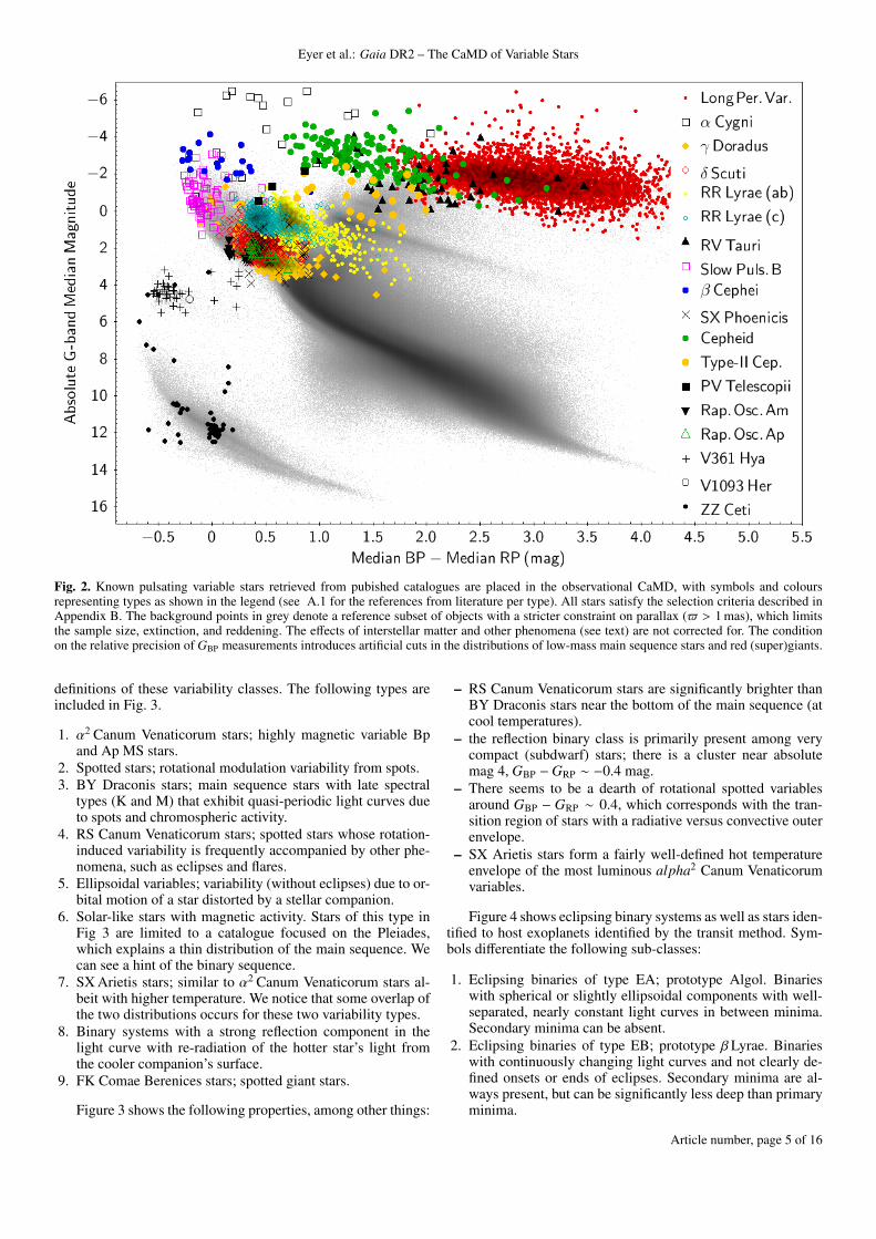
Figure 2 shows the positions of different classes of pulsatingvariable stars based on the Gaia data and can be compared to itstheoretical counterpart in the recent textbooks on asteroseismol-ogy (fig. 1.12 in Aerts et al. 2010) and on pulsating stars (Catelan& Smith 2015). We refer to these books for further details de-scribing specific variability classes. Here, we only consider thefollowing types of pulsating variable stars:

1. Long Period Variables; red giant stars that populate the red-dest and brightest regions of the CaMD. They include Miras,semi-regular variables, slow irregular variables, and smallamplitude red giants.

2. α Cygni stars; luminous supergiant stars that pulsate in non-radial modes. They are particularly affected by interstellarextinction as they are young massive stars residing in theGalactic disc, so their position in Fig. 2 must be treated withcaution.

3. δScuti stars; Population-I stars of spectral types A and F withshort periods (< 0.3 d) that pulsate in dominantly in pressuremodes, but may also reveal low-order gravity modes of lowamplitude.

4. SX Phoenicis stars; Population-II high amplitude δScutistars with periods typically shorter (< 0.2 d) than δScutistars.

5. γDoradus stars; stars with spectral type A and F stars withperiod from 0.3 to 3 d that pulsate dominantly in high-ordergravity modes, but may also reveal low-amplitude pressuremodes.

6. RR Lyrae stars (Bailey’s type ab and c); Population-II hori-zontal branch stars with periods from 0.2 to 1 d that pulsatein pressure mode. C-type RR Lyrae stars are bluer than ab-type stars.

7. Slowly Pulsating B (SPB) stars; non-radial multi-periodicgravity-mode pulsators of spectral type B and with periodstypically in the range from 0.5 to 5 d.

8. β Cephei stars; late O to early-B spectral type non-supergiantstars with dominant low-order pressure and gravity modes,featuring periods in the range from 0.1 to 0.6 d. Several ofthem have been found to also exhibit low-amplitude high-order gravity modes as in the SPB stars (e.g., Stankov &Handler 2005). The β Cephei stars are located in the Galacticdisc so that their CaMD position is easily affected by inter-stellar extinction.

9. Classical Cepheids (prototype δCephei); evolvedPopulation-I (young intermediate-mass) stars featuringradial p-mode pulsations with periods of approximately1 − 100 d. Cepheids can be strongly affected by interstellarextinction as they reside in the Galactic disc and can beobserved at great distances.

10. Type-II Cepheids; Population-II stars pulsating in p-modethat were historically thought to be identical to classi-cal Cepheids. Type-II Cepheids consist of three differentsub-classes (separated by period) commonly referred to asBL Herculis, W Virginis and RV Tauri stars, whose evolu-tionary scenarios differ significantly, although the three sub-classes together define a tight period-luminosity relation.

11. PV Telescopii stars; these include the sub-classes V652 Her,V2076 Oph, and FQ Aqr (Jeffery 2008), which are rarehydrogen-deficient supergiant stars that cover a wide rangeof spectral types and exhibit complex light and radial veloc-ity variations.

12. Rapidly oscillating Am and Ap stars; chemically peculiar Astars that exhibit multiperiodic non-radial pressure modes inthe period range of about 5 − 20 min.

13. V361 Hydrae (or EC 14026) stars; subdwarf B stars on theextreme horizontal branch that pulsate in pressure modeswith very short periods of ∼ 1 − 10 min.

14. V1093 Her (or PG 1716) stars; subdwarf B stars on the ex-treme horizontal branch that pulsate in gravity modes withperiods of 1 − 4 h.

15. ZZ Ceti stars; white dwarfs featuring fast non-radial gravity-mode pulsations with periods of 0.5 − 25 min.

The CaMD of pulsating stars carries a great deal of infor-mation, much of which has shaped the understanding of stellarstructure and evolution and can be found in textbooks. Brieflysummarized, we notice the following particularly interesting fea-tures of Fig. 2.

– Extinction affects variability classes belonging to differentpopulations unequally, as expected. Stars located away fromthe Galactic disk are much less reddened and thus clumpmore clearly. This effect is particularly obvious when com-paring RR Lyrae stars and classical Cepheids, both of whichoccupy the same instability strip, and cannot be explainedby the known fact that the classical instability strip becomeswider in colour at higher luminosity (e.g., see Anderson et al.2016; Marconi et al. 2005; Bono et al. 2000, and referencestherein).

– Interstellar reddening blurs the boundaries between variabil-ity classes. Correcting for interstellar extinction will be cru-cial to delineate the borders of the instability strips in theCaMD, as well as to deduce their purity in terms of the frac-tion of stars that exhibit pulsations while residing in suchregions.

– Practical difficulties involved in separating variable starclasses in the way required to construct Fig. 2 include a) thatvariable stars are often subject to multiple types of variability(e.g. γ Doradus/δ Scuti, β Cephei/SPB hybrid pulsators, pul-sating stars in eclipsing binary systems, or pulsating whitedwarfs that exhibit eruptions), and b) that naming conven-tions are often historical or purely based on light curve mor-phology, so that they do not account for different evolution-ary scenarios (e.g., type-II Cepheids). With additional data,and a fully homogeneous variable star classification basedon Gaia alone, such ambiguities will be resolved in the fu-ture unless they are intrinsically connected to the nature ofthe variability.

– We notice multiple groups of ZZ Ceti stars along the whitedwarf sequence. The most prominent of these is locatedGBP −GRP ' 0 and MG ' 12 as seen in Fontaine & Brassard(2008)

2.2. Variability due to rotation and eclipses

Figure 3 shows stars whose variability is induced by rotation.There are three primary categories: spotted stars, stars deformedby tidal interactions and objects whose variability is due to lightreflected by a companion. Following the nomenclature in theliterature (Table A.1), we list the following variability classesseparately, although we notice occasional overlaps among the



Fig. 2. Known pulsating variable stars retrieved from pubished catalogues are placed in the observational CaMD, with symbols and coloursrepresenting types as shown in the legend (see A.1 for the references from literature per type). All stars satisfy the selection criteria described inAppendix B. The background points in grey denote a reference subset of objects with a stricter constraint on parallax ($ > 1 mas), which limitsthe sample size, extinction, and reddening. The effects of interstellar matter and other phenomena (see text) are not corrected for. The conditionon the relative precision of GBP measurements introduces artificial cuts in the distributions of low-mass main sequence stars and red (super)giants.

definitions of these variability classes. The following types areincluded in Fig. 3.

1. α2 Canum Venaticorum stars; highly magnetic variable Bpand Ap MS stars.

2. Spotted stars; rotational modulation variability from spots.3. BY Draconis stars; main sequence stars with late spectral

types (K and M) that exhibit quasi-periodic light curves dueto spots and chromospheric activity.

4. RS Canum Venaticorum stars; spotted stars whose rotation-induced variability is frequently accompanied by other phe-nomena, such as eclipses and flares.

5. Ellipsoidal variables; variability (without eclipses) due to or-bital motion of a star distorted by a stellar companion.

6. Solar-like stars with magnetic activity. Stars of this type inFig 3 are limited to a catalogue focused on the Pleiades,which explains a thin distribution of the main sequence. Wecan see a hint of the binary sequence.

7. SX Arietis stars; similar to α2 Canum Venaticorum stars al-beit with higher temperature. We notice that some overlap ofthe two distributions occurs for these two variability types.

8. Binary systems with a strong reflection component in thelight curve with re-radiation of the hotter star’s light fromthe cooler companion’s surface.

9. FK Comae Berenices stars; spotted giant stars.

Figure 3 shows the following properties, among other things:

– RS Canum Venaticorum stars are significantly brighter thanBY Draconis stars near the bottom of the main sequence (atcool temperatures).

– the reflection binary class is primarily present among verycompact (subdwarf) stars; there is a cluster near absolutemag 4, GBP −GRP ∼ −0.4 mag.

– There seems to be a dearth of rotational spotted variablesaround GBP − GRP ∼ 0.4, which corresponds with the tran-sition region of stars with a radiative versus convective outerenvelope.

– SX Arietis stars form a fairly well-defined hot temperatureenvelope of the most luminous alpha2 Canum Venaticorumvariables.

Figure 4 shows eclipsing binary systems as well as stars iden-tified to host exoplanets identified by the transit method. Sym-bols differentiate the following sub-classes:

1. Eclipsing binaries of type EA; prototype Algol. Binarieswith spherical or slightly ellipsoidal components with well-separated, nearly constant light curves in between minima.Secondary minima can be absent.

2. Eclipsing binaries of type EB; prototype βLyrae. Binarieswith continuously changing light curves and not clearly de-fined onsets or ends of eclipses. Secondary minima are al-ways present, but can be significantly less deep than primaryminima.



3. Eclipsing binaries of type EW; prototype W Ursae Majoris.The components are nearly or actually in contact and minimaare virtually equally strong. Onsets and ends of minima arenot well defined.

4. Stars known to exhibit exo-planetary transits from the litera-ture.

From Fig. 4, we observe the following:

– EA stars are present almost throughout the CaMD.– We notice groups of EB stars that are overluminous com-

pared to the white dwarf sequence. These are likely whitedwarf stars with main sequence companions.

– The majority of these stars hosting exoplanets are identifiedby Kepler and only very few of them have detectable transitsin the Gaia data, because of different regimes of photometricprecision and time sampling.

2.3. Eruptive and cataclysmic variables

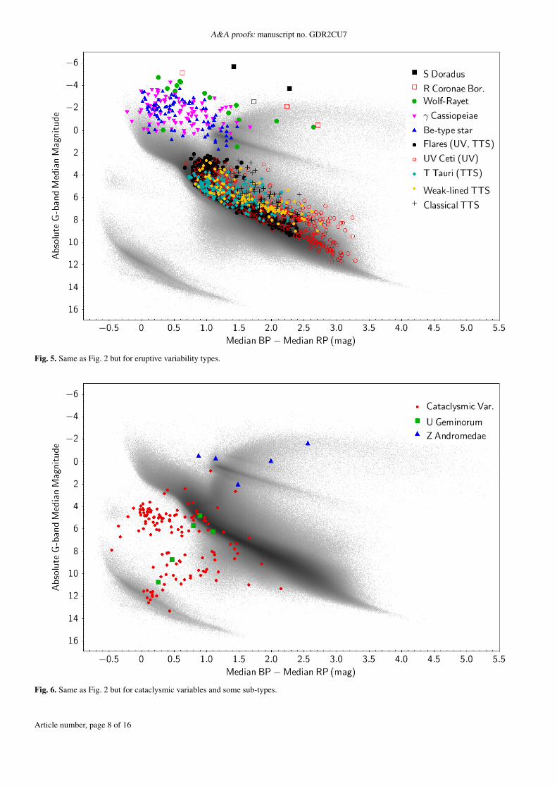
Figure 5 focuses on eruptive variable stars. As for the rotation-ally induced variables, we adopt the nomenclature from the liter-ature (see Table A.1), which includes partially overlapping defi-nitions. The following types are considered.

1. S Doradus stars; Luminous Blue Variables, that is, massiveevolved stars that feature major and irregular photometricvariations due to heavy mass loss by a radiation-driven wind.

2. R Coronae Borealis stars; carbon rich supergiants that emitobscuring material and as a consequence have drastic rapiddimming phases.

3. Wolf-Rayet (WR) stars; the almost naked helium core leftover from originally very high mass evolved stars, featuringstrong emission lines of hydrogen, nitrogen, carbon, or oxy-gen. WR stars are undergoing very fast mass loss and can besignificantly dust-attenuated.

4. γCassiopeiae stars and stars with B spectral types exhibitinghydrogen emission lines, i.e. Be stars; emitting shell stars.During their ‘eruptive’ phenomena, they become brighter.

5. Flare stars; magnetically active stars that display flares. Thiscategory incudes many subtypes of magnetically active stars,such as UV Ceti-type, RS CVn-type, T Tauri stars, etc.

6. UV Ceti stars; usually K-M dwarfs displaying flares.7. T Tauri stars (classical and weak-lined); young pre-main se-

quence stars, either accreting strongly (classical) or show-ing little sign of accretion (weak-lined). Such stars showvariability due to either magnetic activity (e.g., rotationalmodulation, flares) or accretion (quasi-periodic, episodic, orstochastic variations), aside from pulsations that may alsooccur in some of them.

About Fig. 5 we comment on following properties:

– The absence of eruptive variables among hot main sequence(non supergiants) is noticeable. This region is populated bypulsating stars, such as γDoradus and δ Scuti stars, cf. Fig. 2.

– Wolf Rayet stars, R Coronae Borealis stars, and S Doradusstars are among the most luminous stars in this diagram.

Figure 6 illustrates cataclysmic variables:

1. Cataclysmic variables (generic class), typically novae anddwarf novae involving a white dwarf. Many of these starsare situated between the main and white dwarf sequences.

2. U Geminorum stars; dwarf novae, in principle consisting of awhite dwarf with a red dwarf companion experiencing masstransfer.

3. Z Andromedae stars; symbiotic binary stars composed of agiant and a white dwarf.

Further information on cataclysmic variables can be found, e.g.,in Warner (2003) and Hellier (2001).

We notice the following in Fig. 6:

– There is a clump of cataclysmic variables in the ZZ Ceti vari-ability strip location near G ∼ 12 and GBP −GRP ∼ 0.1.

– The most significant clump of cataclysmic variables is nearG ∼ 4 and GBP − GRP ∼ 0.1 mag, they are probably binarysystems with stars from the extreme horizontal branch andthe main sequence.

3. Variable Object Fractions across the CaMD

The different types of brightness variations as presented in theCaMD may strongly depend on the colour and absolute mag-nitude as seen in Sect. 2, because they are driven by differentphysical mechanisms.

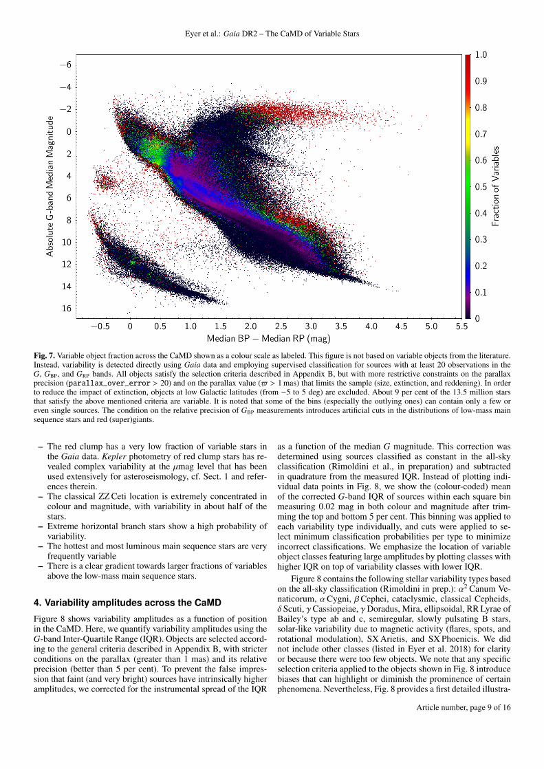
Similarly, the variable object fraction – defined as the num-ber of variable objects per colour-magnitude bin divided by thetotal number of objects in the same bin – is expected to dependon the location in the CaMD. The variable object fraction waspreviously determined based on variable objects detected usingfor example the Hipparcos time series (ESA 1997). Here we sig-nificantly expand this investigation using 13.5 million stars withheliocentric distances of up to 1 kpc that satisfy the astrometricand photometric selection criteria listed in Appendix B as wellas (a) at least 20 observations in the G, GBP, and GRP bands,and (b) a relative parallax error < 5 per cent. In order to reducethe number of objects affected by significant extinction, stars atlow Galactic latitudes (from −5 to 5 deg) are excluded. This ef-fectively reduces the number of disc variables such as classicalCepheids and βCephei stars.

Fig. 7 illustrates this Gaia based high-resolution map ofthe variable object fraction in the CaMD at the precision levelof approximately 5–10 mmag. Variability is identified in about9 per cent of the stars based on a supervised classification ofGaia sources. This method depends heavily on the selection ofthe training set of constant and variable objects. Minor colour-coded features can be due to training-set related biases. The de-tection of variability further depends on the amplitude of thevariables, their apparent magnitude distribution, and the instru-mental precision. The accuracy of the fraction of variables is af-fected also by the number of sources per bin of absolute magni-tude and colour, which can be as low as one in the tails of thetwo-dimensional source number density distribution.

Figure 7 contains many informative features, despite possi-ble biases. Future data releases will significantly improve uponFig. 7 by correcting for reddening and extinction and using largernumber of objects with more accurate source classifications. Forthe time being, we remark that:

– The classical instability strip is clearly visible with variabil-ity in about 50-60 per cent of the stars (although extinctionlimits the precision of this estimate).

– For evolved stars, red giants, and asymptotic giant branchstars, we find that higher luminosity and redder colour im-plies a higher probability of variability.



Fig. 3. Same as Fig. 2 but for rotational-induced variability types.

Fig. 4. Same as Fig. 2 but for eclipsing binaries (of types EA, EB, EW) and known host-stars exhibiting exoplanet transits. As expected, eclipsingbinaries can be anywhere in the CaMD, that explains why they are a main source of contamination for instance of pulsating stars.



Fig. 5. Same as Fig. 2 but for eruptive variability types.

Fig. 6. Same as Fig. 2 but for cataclysmic variables and some sub-types.



Fig. 7. Variable object fraction across the CaMD shown as a colour scale as labeled. This figure is not based on variable objects from the literature.Instead, variability is detected directly using Gaia data and employing supervised classification for sources with at least 20 observations in theG, GBP, and GRP bands. All objects satisfy the selection criteria described in Appendix B, but with more restrictive constraints on the parallaxprecision (parallax_over_error > 20) and on the parallax value ($ > 1 mas) that limits the sample (size, extinction, and reddening). In orderto reduce the impact of extinction, objects at low Galactic latitudes (from −5 to 5 deg) are excluded. About 9 per cent of the 13.5 million starsthat satisfy the above mentioned criteria are variable. It is noted that some of the bins (especially the outlying ones) can contain only a few oreven single sources. The condition on the relative precision of GBP measurements introduces artificial cuts in the distributions of low-mass mainsequence stars and red (super)giants.

– The red clump has a very low fraction of variable stars inthe Gaia data. Kepler photometry of red clump stars has re-vealed complex variability at the µmag level that has beenused extensively for asteroseismology, cf. Sect. 1 and refer-ences therein.

– The classical ZZ Ceti location is extremely concentrated incolour and magnitude, with variability in about half of thestars.

– Extreme horizontal branch stars show a high probability ofvariability.

– The hottest and most luminous main sequence stars are veryfrequently variable

– There is a clear gradient towards larger fractions of variablesabove the low-mass main sequence stars.

4. Variability amplitudes across the CaMD

Figure 8 shows variability amplitudes as a function of positionin the CaMD. Here, we quantify variability amplitudes using theG-band Inter-Quartile Range (IQR). Objects are selected accord-ing to the general criteria described in Appendix B, with stricterconditions on the parallax (greater than 1 mas) and its relativeprecision (better than 5 per cent). To prevent the false impres-sion that faint (and very bright) sources have intrinsically higheramplitudes, we corrected for the instrumental spread of the IQR

as a function of the median G magnitude. This correction wasdetermined using sources classified as constant in the all-skyclassification (Rimoldini et al., in preparation) and subtractedin quadrature from the measured IQR. Instead of plotting indi-vidual data points in Fig. 8, we show the (colour-coded) meanof the corrected G-band IQR of sources within each square binmeasuring 0.02 mag in both colour and magnitude after trim-ming the top and bottom 5 per cent. This binning was applied toeach variability type individually, and cuts were applied to se-lect minimum classification probabilities per type to minimizeincorrect classifications. We emphasize the location of variableobject classes featuring large amplitudes by plotting classes withhigher IQR on top of variability classes with lower IQR.

Figure 8 contains the following stellar variability types basedon the all-sky classification (Rimoldini in prep.): α2 Canum Ve-naticorum, αCygni, βCephei, cataclysmic, classical Cepheids,δScuti, γCassiopeiae, γDoradus, Mira, ellipsoidal, RR Lyrae ofBailey’s type ab and c, semiregular, slowly pulsating B stars,solar-like variability due to magnetic activity (flares, spots, androtational modulation), SX Arietis, and SX Phoenicis. We didnot include other classes (listed in Eyer et al. 2018) for clarityor because there were too few objects. We note that any specificselection criteria applied to the objects shown in Fig. 8 introducebiases that can highlight or diminish the prominence of certainphenomena. Nevertheless, Fig. 8 provides a first detailed illustra-



Fig. 8. Amplitude of variability in the CaMD, from a selection of classified variables within 1 kpc and with a relative uncertainty for the parallaxof 5 per cent. The colour scale shows the corrected G-band IQR (see text) with a cut-off at 0.1 mag to emphasize the low and mid-level variability.The background points in grey represent classified constant stars. All objects satisfy the selection criteria described in Appendix B, in addition tothe stricter conditions on parallax and its precision as mentioned above. The effects of interstellar extinction are not corrected for.

tion of some of the most important amplitude-related variabilityfeatures across the CaMD. A number of clumps and instabilityregions are visible in Fig. 8, which are related to the variabil-ity classes described in Sects. 2 and 3. We notice the followingtrends and concentrations:

– The classical instability strip containing classical Cepheidsand RR Lyrae stars is not very prominent, although someclumps (in red or cyan) are apparent.

– The instability regions linked to SPB stars and βCephei starsare broad and uniform.

– Higher amplitude variations are clearly correlated with red-der colours for long period variables.

– The highest amplitude (IQR > 0.1 mag) variables occur inseveral regions across the CaMD, including the classical in-stability strip, long period variables, below the red clump,above the main sequence of low-mass stars (in correspon-dence of the observed gradient in the fraction of variables),and between the white dwarfs sequence and the main se-quence.

– Significant amplitudes of > 0.04 mag are found very fre-quently among the coolest white dwarfs.

– The stars between the main sequence and the white dwarfssequence feature large variability amplitudes and extend intothe clump of ZZ Ceti stars in the white dwarf sequence. This

intermediate region is populated in particular by the high-amplitude cataclysmic variables, cf. Fig. 6. A closeup viewof the white dwarf sequence is shown in Fig. 9, which rep-resents all classified variables within 200 pc, plotting eachobject without binning, in order to emphasize the variabilityof the ZZ Ceti stars.

5. Variability-induced motion in the CaMD

In this Section, we visualise the variability-induced motion ofstars across the time-dependent CaMD using all-sky measure-ments made in the G, GBP, and GRP passbands. Gaia data areuniquely suited to create this time-dependent CaMD, since thedifferent data types – astrometric, photometric in three-band –are acquired in a quasi-simultaneous fashion at many epochsdistributed over a multi-year time span. The first of such rep-resentations, although much less detailed, was first presented forindividual classical Cepheids in the Milky Way (Eggen 1951)and in Galactic star clusters (Kholopov 1956; Sandage 1958).Similarly minded representations in the literature were based ondata from the SDSS (Ivezic et al. 2003, mostly Galactic objects),EROS (Spano et al. 2009, LMC objects), and, very recently, theHST observations of M51 (Conroy et al. 2018).



Fig. 9. Same as Fig. 8 but focusing on the white dwarf sequence andplotting all classified variables within 200 pc with a relative uncertaintyfor the parallax better than 5 per cent. A close inspection of this se-quence reveals amplitudes at the level of 40 mmag in various regions.

Figure 10 illustrates the variability-induced motion of starsin the CaMD. As elsewhere in this paper, no correction for in-terstellar extinction is applied. Individual stars are shown by dif-ferently (arbitrarily) coloured lines that connect successive ab-solute G magnitudes and GBP −GRP measurements, i.e., the ob-servations are ordered in time as opposed to variability phase.This choice was made to avoid uncertainties related to phase-folding the relatively sparsely-sampled light curves based on 22or fewer months of observations and to include both periodic andnon-periodic variable objects.

Figure 10 is limited to a subset of all available variablestars in order to avoid overcrowding the diagram. As a pre-view for future data releases, we include here the variability-induced motions of some stars whose time series and variabilitytypes are not published in DR2 (but available as online mate-rial). Figure 10 includes the following variability types definedin Sec. 2: α2 Canum Venaticorum variables, B-type emission line/γCassiopeiae stars, cataclysmic variables, classical and type-IICepheids, δScuti stars, eclipsing binaries, RR Lyrae stars, longperiod variables, and SX Phoenicis stars. All sources shown sat-isfy the general criteria described in Appendix B and typicallyhave at least 10 observations available 1. We further prioritizedthe selection of objects featuring larger ranges of variations inthe G band (with a minimum of about 0.1 mag)2. The numberof sources shown per variability type ranges from a few to sev-eral tens and was selected to ensure clarity in case of high sourcedensity or overlapping variability classes in certain regions of theCaMD. In order to limit the effect of outlying values, time seriesdata are filtered by operators as described in Holl et al. (in prep.),and the 10 per cent brightest and faintest observations in the GRPband are excluded for sources with GBP −GRP less than 1.5 mag.Non-variable objects are shown as a grey background to providea visual reference for the variable object locations in the CaMD.These stars satisfy the criteria described in Appendix B as well

1 The minimum number of observations per source is increased to 20in the case of long period variables, but the condition on the number ofobservations is removed for cataclysmic variables.2 A minimum range in the G band is not required for α2 Canum Venati-corum stars and cataclysmic variables as their variability may be smallin the ‘white’ G band

as the stricter condition of $ > 1 mas. Stars whose variabilityis caused by different physical effects exhibit different motionswithin the time-dependent CaMD. We briefly summarize the dif-ferent motions seen in Fig.10 as follow.

1. Pulsating stars, including long period variables, Cepheids,RR Lyrae, and δScuti/SX Phoenicis stars exhibit a similarbehaviour. These stars are bluer when brighter in G, whichillustrates that brightness variations of pulsating stars aredominated by the effect of change in temperature rather thanradius. For the longest-period variables, the 22 month timespan of the Gaia data is similar to the pulsation cycle, sothat in some cases loop-like shapes are apparent. For variablestars with shorter periods (e.g., RR Lyrae stars or classicalCepheids), successive measurements in time are not gener-ally ordered in phase, so that an overall ‘envelope’ of manycycles is revealed.

2. The motions of eclipsing binary systems in the CaMD de-pends on the colour difference between the two stars. Thecomponents of eclipsing systems of the EW type have sim-ilar mass (and colour), leading to a rather vertically alignedmotion (parallel to the absolute magnitude axis). For eclips-ing binary systems with stars of different mass (and thuscolour) close to the main sequence, the deepest eclipse isusually slightly redder, since the secondary (less massiveand redder) component eclipses part of the light of the pri-mary star. The slope of the motion of eclipsing binaries inthe CaMD is very different (much steeper) than the one ofpulsating stars.

3. Rotationally induced variables (shown here: α2 Canum Ve-naticorum stars) feature small amplitudes in absolute G andare rather horizontal in the CaMD. This is as expected fromstarspots, which have lower temperature than the surround-ing and hence absorb the light at bluer frequencies to re-emitit by back warming effect at redder frequencies. Therefore,the magnitude change in a broad band like G is smaller thanit would be if measured in narrow bands.

4. Eruptive stars (shown here: γCassiopeiae and Be-type stars)become redder when brighter, because of additional extinc-tion during their eruptive phase. Hence, the slopes of theirmotions in the CaMD have the opposite sign with respect tothe one of pulsating stars.

5. The variability of cataclysmic variables (shown here: novae)primarily features strong outbursts in the ultraviolet and bluepart of the spectrum that are understood to be caused by masstransfer from donor stars in binary systems. These outburstschange very significantly the colour of the system towardsbluer values.

The current version of Fig. 10 represents a first step towardsa more global description of stellar variability. The motions de-scribed by the variable stars in the time-dependent CaMD pro-vide new perspectives on the data that can be exploited as vari-able star classification attributes to appreciably improve the clas-sification results. Gaia data will definitively help identify mis-classifications and problems in published catalogues, thanks toits astrometry and the quasi-simultaneous measurements.

In future Gaia data releases, there will be more data pointsper source, making it possible to refine Fig. 10. In particular,periods can be determined with an accuracy inversely propor-tional to the total Gaia time base for periodic objects. That way,the motion in the CaMD can be represented more precisely byconnecting points sorted in phase (rather than in time), leadingto Lissajous-type configurations for pulsators. For sufficiently



Fig. 10. Motions of selected variable stars in the CaMD, highlighted by segments connecting successive absolute G magnitudes and GBP − GRPmeasurements in time with the same colour for the same source. Preferential directions and amplitudes of magnitude and colour variations can beinferred as a function of variability type (α2 Canum Venaticorum, Be-type and γCassiopeiae, cataclysmic, classical and type-II Cepheid, δScutiand SX Phoenicis, eclipsing binary, long period, and RR Lyrae), as labelled in the Figure. For clarity of visualization, the selection of eclipsingbinaries (and partially other types) was adjusted to minimize the overlap with other types. Selection criteria of all sources represented in colour orgrey are the same as in Fig. 2. Additional conditions are described in the text.



bright stars, radial velocity time series will add a third and un-precedented dimension to Fig. 10.

An animated version of Fig. 10 is provided at https://www.cosmos.esa.int/web/gaia/gaiadr2_cu7.

6. Conclusions

The Gaia mission enables a comprehensive description of phe-nomena related to stellar variability. In this paper, we have fo-cused on stellar variability across the CaMD, showcasing loca-tions occupied by different variability types as well as variableobject fractions, variability amplitudes, and variability-inducedmotions described by different variability classes across theCaMD.

The wealth of information related to variable stars and con-tained in Gaia DR2 is unprecedented for the Milky Way. TheCaMD can provide guidance for further detailed studies, whichcan focus on individual regions or clumps, e.g. to investigatethe purity of instability strips and how sharply such regionsare truly defined or how they depend on chemical composition.Of course, additional work is required to this end, and accu-rately correcting for reddening and extinction will be crucial.The (time-dependent) CaMD will play an important role for im-proving variable star classification by providing additional at-tributes, such as the expected direction of variability for specificvariable classes, and for illustrating stellar variability to non-expert audiences.

The CaMD of variable stars can further point out interre-lations between variability phenomena that are otherwise noteasily recognized and possibly identify new types of variabil-ity. Detailed follow-up observations from the ground will helpcorrect previous misclassifications and in-depth studies of pe-culiar and particularly interesting objects. Thanks to the pre-sented variable stars residing in the Milky Way, it will be pos-sible to obtain particularly high signal-to-noise data, e.g. usinghigh-resolution spectroscopy. Finally, the observed properties ofvariable stars in the CaMD, such as instability strip boundariesor period-luminosity relations, provide crucial input and con-straints for models describing pulsational instability, convection,and stellar structure in general.

Future Gaia data releases will further surpass the variabil-ity content of this second data release3. By the end of mission,Gaia data are expected to comprise many tens of millions ofvariable celestial objects, including many additional variabilitytypes, as well as time series BP and RP spectra. Eventually, timeseries of radial velocities and spectra from the radial velocityspectrometer will be published for subsets of variables. Finally,the variability classification of future Gaia data will also makeuse of unsupervised clustering techniques aimed at discoveringentirely new (sub-)clusters and classes of variable phenomena.

Acknowledgements. We would like to thank Laurent Rohrbasser for tests doneon the representation of time series. This work has made use of data fromthe ESA space mission Gaia, processed by the Gaia Data Processing andAnalysis Consortium (DPAC). Funding for the DPAC has been providedby national institutions, some of which participate in the Gaia MultilateralAgreement, which include, for Switzerland, the Swiss State Secretariat forEducation, Research and Innovation through the ESA Prodex program, the“Mesures d’accompagnement”, the “Activités Nationales Complémentaires”, theSwiss National Science Foundation, and the Early Postdoc.Mobility fellowship;for Belgium, the BELgian federal Science Policy Office (BELSPO) throughPRODEX grants; for Italy, Istituto Nazionale di Astrofisica (INAF) and theAgenzia Spaziale Italiana (ASI) through grants I/037/08/0, I/058/10/0, 2014-025-R.0, and 2014-025-R.1.2015 to INAF (PI M.G. Lattanzi); for France, theCentre National d’Etudes Spatiales (CNES). Part of this research has received

3 cf. https://www.cosmos.esa.int/web/gaia/release

funding from the European Research Council (ERC) under the European Union’sHorizon 2020 research and innovation programme (Advanced Grant agreementsN◦670519: MAMSIE “Mixing and Angular Momentum tranSport in MassIvEstars”).This research has made use of NASA’s Astrophysics Data System, the VizieRcatalogue access tool, CDS, Strasbourg, France, and the International VariableStar Index (VSX) database, operated at AAVSO, Cambridge, Massachusetts,USA.We gratefully acknowledge Mark Taylor for creating the astronomy-orienteddata handling and visualization software TOPCAT (Taylor 2005).


https://www.cosmos.esa.int/web/gaia/gaiadr2_cu7

https://www.cosmos.esa.int/web/gaia/gaiadr2_cu7

https://www.cosmos.esa.int/web/gaia/release


Appendix A: Literature per variability type

See Table A.1 for details on the references from literature re-garding the objects included in Figs. 2–6 and 10.

Appendix B: Selection criteria

Astrometric and photometric conditions are applied to allCaMDs for improved accuracy of the star locations in such di-agrams. Astrometric constraints include limits on the numberof visibility periods (observation groups separated from othergroups by at least four days) per source used in the secondaryastrometric solution (Gaia Collaboration et al. 2018), the excessastrometric noise of the source postulated to explain the scatterof residuals in the astrometric solution for that source (Gaia Col-laboration et al. 2018), and the relative parallax precision (hereinset to 5 but increased up to 20 in some applications):

1. visibility_periods_used > 5;2. astrometric_excess_noise < 0.5 mas;3. parallax > 0 mas;4. parallax_over_error > 5.

Photometric conditions set limits for each source on the relativeprecisions of the mean fluxes in the GBP, GRP, and G bands, aswell as on the mean flux excess in the GBP and GRP bands withrespect to the G band as a function of colour (Evans et al. 2018):

5. phot_bp_mean_flux_error / phot_bp_mean_flux< 0.05;6. phot_rp_mean_flux_error / phot_rp_mean_flux< 0.05;7. phot_g_mean_flux_error / phot_g_mean_flux < 0.02;8. (phot_bp_mean_flux + phot_rp_mean_flux) /

{phot_g_mean_flux * [1.2 + 0.03 * (phot_bp_mean_mag- phot_rp_mean_mag)2]} < 1.2.

The ADQL query to select a sample of sources that satisfyall of the above listed criteria follows.

SELECT TOP 10 source_idFROM gaiadr2.gaia_sourceWHERE visibility_periods_used > 5AND astrometric_excess_noise < 0.5AND parallax > 0AND parallax_over_error > 5AND phot_bp_mean_flux_over_error > 20AND phot_rp_mean_flux_over_error > 20AND phot_g_mean_flux_over_error > 50AND phot_bp_rp_excess_factor < 1.2*(1.2+0.03*

power(phot_bp_mean_mag-phot_rp_mean_mag,2))

ReferencesAbbas, M., Grebel, E. K., Martin, N. F., et al. 2014, AJ, 148, 8Aerts, C. 2015, in IAU Symposium, Vol. 307, New Windows on Massive Stars,

ed. G. Meynet, C. Georgy, J. Groh, & P. Stee, 154–164Aerts, C., Christensen-Dalsgaard, J., & Kurtz, D. W. 2010, Asteroseismology,

Astronomy and Astrophysics Library (Springer Science+Business MediaB.V.)

Alcock, C., Allsman, R. A., Axelrod, T. S., et al. 1993, in Astronomical Societyof the Pacific Conference Series, Vol. 43, Sky Surveys. Protostars to Proto-galaxies, ed. B. T. Soifer, 291

Alfonso-Garzón, J., Domingo, A., Mas-Hesse, J. M., & Giménez, A. 2012,A&A, 548, A79

Anderson, R. I., Saio, H., Ekström, S., Georgy, C., & Meynet, G. 2016, A&A,591

Arenou, F., Luri, X., Babusiaux, C., & et al. 2018, e-printAuvergne, M., Bodin, P., Boisnard, L., et al. 2009, A&A, 506, 411Bedding, T. R., Mosser, B., Huber, D., et al. 2011, Nature, 471, 608

Bellm, E. 2014, in The Third Hot-wiring the Transient Universe Workshop, ed.P. R. Wozniak, M. J. Graham, A. A. Mahabal, & R. Seaman, 27–33

Bono, G., Castellani, V., & Marconi, M. 2000, ApJ, 529, 293Bowman, D. M. 2017, Amplitude Modulation of Pulsation Modes in Delta Scuti

Stars, Jeremiah Horrocks Institute, University of Central Lancashire, Preston,UK. (PhD Thesis) (Springer Thesis series)

Braga, V. F., Stetson, P. B., Bono, G., et al. 2016, AJ, 152, 170Casertano, S., Riess, A. G., Bucciarelli, B., & Lattanzi, M. G. 2017, A&A, 599,

A67Catelan, M. & Smith, H. A. 2015, Pulsating Stars (Wiley-VCH)Chang, S.-W., Byun, Y.-I., & Hartman, J. D. 2015, ApJ, 814, 35Chaplin, W. J. & Miglio, A. 2013, ARA&A, 51, 353Conroy, C., Strader, J., van Dokkum, P., et al. 2018, ArXiv e-printsDe Ridder, J., Molenberghs, G., Eyer, L., & Aerts, C. 2016, A&A, 595, L3Debosscher, J., Blomme, J., Aerts, C., & De Ridder, J. 2011, A&A, 529, A89Debosscher, J., Sarro, L. M., Aerts, C., et al. 2007, A&A, 475, 1159Drake, A. J., Catelan, M., Djorgovski, S. G., et al. 2013a, ApJ, 763, 32Drake, A. J., Catelan, M., Djorgovski, S. G., et al. 2013b, ApJ, 765, 154Drake, A. J., Gänsicke, B. T., Djorgovski, S. G., et al. 2014a, MNRAS, 441, 1186Drake, A. J., Graham, M. J., Djorgovski, S. G., et al. 2014b, ApJS, 213, 9Eggen, O. J. 1951, ApJ, 113, 367EROS Collaboration, Derue, F., Afonso, C., et al. 1999, A&A, 351, 87ESA, ed. 1997, ESA Special Publication, Vol. 1200, The Hipparcos and Ty-

cho catalogues. Astrometric and photometric star catalogues derived from theESA Hipparcos Space Astrometry Mission

Evans, D., Riello, M., De Angeli, F., & et al. 2018, e-printEyer, L. & Grenon, M. 1997, in ESA Special Publication, Vol. 402, Hipparcos -

Venice ’97, ed. R. M. Bonnet, E. Høg, P. L. Bernacca, L. Emiliani, A. Blaauw,C. Turon, J. Kovalevsky, L. Lindegren, H. Hassan, M. Bouffard, B. Strim,D. Heger, M. A. C. Perryman, & L. Woltjer, 467–472

Eyer, L., Grenon, M., Falin, J.-L., Froeschle, M., & Mignard, F. 1994, Sol. Phys.,152, 91

Eyer, L., Guy, L., & Rimoldini, L. e. a. 2018, Gaia DR1 documentation Chapter6: Variability, Tech. rep., Gaia DPAC; European Space Agency

Eyer, L. & Mowlavi, N. 2008, Journal of Physics Conference Series, 118, 012010Eyer, L., Palaversa, L., Mowlavi, N., et al. 2012, Ap&SS, 341, 207Fontaine, G. & Brassard, P. 2008, PASP, 120, 1043Gaia Collaboration, Babusiaux, C., van Leeuwen, F., Barstow, M., & et al. 2018,

e-printGaia Collaboration, Brown, A. G. A., Vallenari, A., et al. 2016a, A&A, 595, A2Gaia Collaboration, Clementini, G., Eyer, L., & et al. 2017, A&A, 605, A79Gaia Collaboration, Prusti, T., de Bruijne, J. H. J., et al. 2016b, A&A, 595, A1Gilliland, R. L., Brown, T. M., Christensen-Dalsgaard, J., et al. 2010, PASP, 122,

131Hartman, J. D., Bakos, G. Á., Kovács, G., & Noyes, R. W. 2010, MNRAS, 408,

475Hekker, S. & Christensen-Dalsgaard, J. 2017, A&A Rev., 25, 1Hellier, C. 2001, Cataclysmic Variable Stars (Springer)Hermes, J. J., Kawaler, S. D., Romero, A. D., et al. 2017, ApJ, 841, L2Holl et al. in prep., Gaia Data Release 2 – Variability Processing and Analysis

ResultsHowell, S. B., Sobeck, C., Haas, M., et al. 2014, PASP, 126, 398Huber, D., Zinn, J., Bojsen-Hansen, M., et al. 2017, ApJ, 844, 102Ivezic, Ž., Lupton, R. H., Anderson, S., et al. 2003, Mem. Soc. Astron. Italiana,

74, 978Jeffery, C. S. 2008, Information Bulletin on Variable Stars, 5817Kahraman Aliçavus, F., Niemczura, E., De Cat, P., et al. 2016, MNRAS, 458,

2307Kholopov, P. N. 1956, Peremennye Zvezdy, 11, 325Kinemuchi, K., Smith, H. A., Wozniak, P. R., McKay, T. A., & ROTSE Collab-

oration. 2006, AJ, 132, 1202Leavitt, H. S. 1908, Annals of Harvard College Observatory, 60, 87Leavitt, H. S. & Pickering, E. C. 1912, Harvard College Observatory Circular,

173, 1LSST Science Collaboration, Abell, P. A., Allison, J., et al. 2009, ArXiv e-printsMarconi, M., Musella, I., & Fiorentino, G. 2005, ApJ, 632, 590Mróz, P., Udalski, A., Poleski, R., et al. 2015, Acta Astron., 65, 313Niemczura, E. 2003, A&A, 404, 689Pablo, H., Whittaker, G. N., Popowicz, A., et al. 2016, PASP, 128, 125001Palaversa, L., Ivezic, Ž., Eyer, L., et al. 2013, AJ, 146, 101Perryman, M. A. C., Lindegren, L., Kovalevsky, J., et al. 1997, A&A, 323Pigulski, A., Pojmanski, G., Pilecki, B., & Szczygieł, D. M. 2009, Acta Astron.,

59, 33Rauer, H., Catala, C., Aerts, C., et al. 2014, Experimental Astronomy, 38, 249Reinhold, T. & Gizon, L. 2015, A&A, 583, A65Richards, J. W., Starr, D. L., Miller, A. A., et al. 2012, Astrophys. J. Suppl.

Series, 203, 32Ricker, G. R., Winn, J. N., Vanderspek, R., et al. 2015, Journal of Astronomical

Telescopes, Instruments, and Systems, 1, 014003



Table A.1. Literature references of stars as a function of variability type and the corresponding number of sources depicted in Figs. 2–6, afterselections based on reliability, photometric accuracy, and astrometric parameters (Appendix B). Figure 10 includes only subsets of variability typesand of sources per type.

Variability Type Reference # Sources

Pulsating α Cygni Hip97, VSX16 17β Cephei PDC05 20Cepheid ASA09, Hip97, INT12 155δ Scuti ASA09, Hip97, JD07, Kep11b, Kep11c, SDS12 724γ Doradus FKA16, Kep11b, Kep11c, VSX16 561Long Period Variable ASA12, Hip97, INT12, Kep11b, NSV04 5221PV Telescopii VSX16 3Rapidly Oscillating Am star VSX16 8Rapidly Oscillating Ap star VSX16 25RR Lyrae, fundamental mode (RRab) ASA09, ASA12, Cat13a, Cat13b, Cat14b, Cat15, Hip97, 1676

INT12, LIN13, NSV06, VFB16, VSX16RR Lyrae, first overtone (RRc) ASA09, ASA12, Cat13b, Cat14b, Hip97, INT12, Kep11b, 611

LIN13, MA14, VFB16, VSX16RV Tauri ASA12, Hip97, VSX16 48Slowly Pulsating B star IUE03, Hip97, PDC05 78SX Phoenicis ASA12, Hip97, VSX16 41Type-II Cepheid ASA12, Cat14b, Hip97, VSX16 21V361 Hya (also EC 14026) VSX16 41V1093 Her (also PG 1716) VSX16 1ZZ Ceti VSX16 61

Rotational α2 Canum Venaticorum Hip97, VSX16 598Binary with Reflection VSX16 27BY Draconis VSX16 713Ellipsoidal ASA12, Cat14b, Hip97, Kep11b, VSX16 398FK Comae Berenices Hip97 3Rotating Spotted Kep15b 16 593RS Canum Venaticorum ASA12, Cat14b, Hip97, VSX16 1381Solar-Like Variations HAT10 176SX Arietis Hip97, VSX16 14

Eclipsing EA, β Persei (Algol) ASA09, Cat14b, Hip97, LIN13, VSX16 8123EB, β Lyrae ASA09, Cat14b, Hip97, LIN13, VSX16 3096EW, W Ursae Majoris ASA09, Hip97, VSX16 3248Exoplanet JS15 278

Eruptive B-type emission-line star ASA12, VSX16 86Classical T Tauri Star VSX16 75Flares (UV, BY, TTS) Kep11a, Kep13, Kep15a, MMT15 478γ Cassiopeiae Hip97, VSX16 84R Coronae Borealis VSX16 4S Doradus ASA12, INT12 2T Tauri Star (TTS) VSX16 173UV Ceti INT12, VSX16 425Weak-lined T Tauri Star VSX16 119Wolf-Rayet INT12, VSX16 15

Cataclysmic Cataclysmic Variable (generic) Cat14a, OGL15, VSX16 132U Geminorum INT12, VSX16 4Z Andromedae INT12, VSX16 5

Notes. ASA09: Pigulski et al. (2009); ASA12: Richards et al. (2012); Cat13a: Drake et al. (2013a); Cat13b: Drake et al. (2013b); Cat14a: Drakeet al. (2014a); Cat14b: Drake et al. (2014b); Cat15: Torrealba et al. (2015); FKA16: Kahraman Aliçavus et al. (2016); HAT10: Hartman et al.(2010); Hip97: ESA (1997); INT12: Alfonso-Garzón et al. (2012); IUE03: Niemczura (2003); JD07: Debosscher et al. (2007); JS15: J. South-worth, http://www.astro.keele.ac.uk/jkt/tepcat/observables.html (as of Aug. 2015); Kep11a: Walkowicz et al. (2011); Kep11b:Debosscher et al. (2011); Kep11c: Uytterhoeven et al. (2011); Kep13: Shibayama et al. (2013); Kep15a: Wu et al. (2015); Kep15b: Reinhold &Gizon (2015); LIN13: Palaversa et al. (2013); MA14: Abbas et al. (2014); MMT15: Chang et al. (2015); NSV04: Wozniak et al. (2004); NSV06:Kinemuchi et al. (2006); OGL15: Mróz et al. (2015); PDC05: P. De Cat, http://www.ster.kuleuven.ac.be/~peter/Bstars/ (as of Jan.2005); SDS12: Süveges et al. (2012); VFB16: Braga et al. (2016); VSX16: Watson et al. (2016, 2015, 2006).


http://www.astro.keele.ac.uk/jkt/tepcat/observables.html

http://www.ster.kuleuven.ac.be/~peter/Bstars/


Roelens, M., Eyer, L., Mowlavi, N., et al. in prep., Gaia Data Release 2 – TheShort Timescale Variability Processing and Analysis

Sandage, A. 1958, ApJ, 128, 150Shibayama, T., Maehara, H., Notsu, S., et al. 2013, ApJS, 209, 5Spano, M., Mowlavi, N., Eyer, L., & Burki, G. 2009, in American Institute of

Physics Conference Series, Vol. 1170, American Institute of Physics Confer-ence Series, ed. J. A. Guzik & P. A. Bradley, 324–326

Stankov, A. & Handler, G. 2005, ApJS, 158, 193Süveges, M., Sesar, B., Váradi, M., et al. 2012, MNRAS, 424, 2528Taylor, M. B. 2005, in Astronomical Society of the Pacific Conference Se-

ries, Vol. 347, Astronomical Data Analysis Software and Systems XIV, ed.P. Shopbell, M. Britton, & R. Ebert, 29

Torrealba, G., Catelan, M., Drake, A. J., et al. 2015, MNRAS, 446, 2251Udalski, A., Szymanski, M. K., & Szymanski, G. 2015, Acta Astron., 65, 1Uytterhoeven, K., Moya, A., Grigahcène, A., et al. 2011, A&A, 534, A125van Leeuwen, F., Evans, D. W., De Angeli, F., et al. 2017, A&A, 599, A32Walkowicz, L. M., Basri, G., Batalha, N., et al. 2011, AJ, 141, 50Warner, B. 2003, Cataclysmic Variable Stars (Cambridge University Press)Watson, C. L., Henden, A. A., & Price, A. 2006, Society for Astronomical Sci-

ences Annual Symposium, 25, 47Watson, C. L., Henden, A. A., & Price, A. 2015, CDS/ADC Collection of Elec-

tronic Catalogues, 1, 2027Watson, C. L., Wils, P., & Ochsenbein, O. 2016, VizieR Online Data Catalogue,

VSX Version 2016-07-04Wozniak, P. R., Williams, S. J., Vestrand, W. T., & Gupta, V. 2004, AJ, 128, 2965Wu, C.-J., Ip, W.-H., & Huang, L.-C. 2015, ApJ, 798, 92

1 Department of Astronomy, University of Geneva, Ch. des Maillettes51, CH-1290 Versoix, Switzerland

2 Department of Astronomy, University of Geneva, Ch. d’Ecogia 16,CH-1290 Versoix, Switzerland

3 European Southern Observatory, Karl-Schwarzschild-Str. 2, D-85748 Garching b. München, Germany

4 SixSq, Rue du Bois-du-Lan 8, CH-1217 Geneva, Switzerland5 GÉPI, Observatoire de Paris, Université PSL, CNRS, Place Jules

Janssen 5, F-92195 Meudon, France6 INAF Osservatorio di Astrofisica e Scienza dello Spazio di Bologna,

Via Gobetti 93/3, I - 40129 Bologna, Italy7 Instituut voor Sterrenkunde, KU Leuven, Celestijnenlaan 200D,

3001 Leuven, Belgium8 Institute of Astronomy, University of Cambridge, Madingley Road,

Cambridge CB3 0HA, UK9 Large Synoptic Survey Telescope, 950 N. Cherry Avenue, Tucson,

AZ 85719, USA10 Università di Catania, Dipartimento di Fisica e Astronomia, Sezione

Astrofisica, Via S. Sofia 78, I-95123 Catania, Italy11 INAF-Osservatorio Astrofisico di Catania, Via S. Sofia 78, I-95123

Catania, Italy12 University of Vienna, Department of Astrophysics, Tuerkenschanz-

strasse 17, A1180 Vienna, Austria13 Department of Geosciences, Tel Aviv University, Tel Aviv 6997801,

Israel14 Dipartimento di Fisica e Astronomia, Università di Bologna, Via

Piero Gobetti 93/2, 40129 Bologna, Italy15 Departamento de Astrofísica, Centro de Astrobiología (INTA-

CSIC), PO Box 78, E-28691 Villanueva de la Cañada, Spain16 School of Physics and Astronomy, Tel Aviv University, Tel Aviv

6997801, Israel17 INAF-Osservatorio Astronomico di Capodimonte, Via Moiariello

16, 80131, Napoli, Italy18 Dpto. Inteligencia Artificial, UNED, c/ Juan del Rosal 16, 28040

Madrid, Spain19 Department of Astrophysics/IMAPP, Radboud University, P.O.Box

9010, 6500 GL Nijmegen, The Netherlands20 Laboratoire d’astrophysique de Bordeaux, Univ. Bordeaux, CNRS,

B18N, allée Geoffroy Saint-Hilaire, 33615 Pessac, France21 Harvard-Smithsonian Center for Astrophysics, 60 Garden Street,

Cambridge, MA 02138, USA22 Royal Observatory of Belgium, Ringlaan 3, B-1180 Brussels, Bel-

gium23 Konkoly Observatory, Research Centre for Astronomy and Earth

Sciences, Hungarian Academy of Sciences, H-1121 Budapest,Konkoly Thege Miklós út 15-17, Hungary.

24 Department of Astronomy, Eötvös Loránd University, PázmányPéter sétány 1/a, H-1117, Budapest, Hungary

25 Villanova University, Department of Astrophysics and PlanetaryScience, 800 Lancaster Ave, Villanova PA 19085, USA

26 A. Kochoska Faculty of Mathematics and Physics, University ofLjubljana, Jadranska ulica 19, 1000 Ljubljana, Slovenia

27 Academy of Sciences of the Czech Republic, Fricova 298, 25165Ondrejov, Czech Republic

28 Baja Observatory of University of Szeged, Szegedi út III/70, H-6500Baja, Hungary.

29 Université Côte d’Azur, Observatoire de la Côte d’Azur, CNRS,Laboratoire Lagrange, Bd de l’Observatoire, CS 34229, 06304 Nicecedex 4, France

30 CENTRA FCUL, Campo Grande, Edif. C8, 1749-016 Lisboa, Por-tugal

31 EPFL SB MATHAA STAP, MA B1 473 (Bâtiment MA), Station 8,CH-1015 Lausanne, Switzerland

32 Warsaw University Observatory, Al. Ujazdowskie 4, 00-478Warszawa, Poland

33 Institute of Theoretical Physics, Faculty of Mathematics andPhysics, Charles University in Prague, Czech Republic

34 Max Planck Institute for Astronomy, Königstuhl 17, 69117 Heidel-berg, Germany


variable stars in the colour-absolute magnitude diagram · variable stars in the colour-absolute...

Documents