variance reduction schemes for monte carlo estimators...
TRANSCRIPT

Variance reduction schemes for Monte Carlo estimators in
globalillumination algorithms
László Szécsi
Budapest University of Technology

Scope of this talk
• the rendering problem– as an integral equation
• examples from our previous work– how Monte-Carlo variance reduction
techniques translate to better global illumination rendering algorithms
• overview– instead of detailed analysis

The rendering problem
• Find the radiance toward the eye from surface element visible in pixels
L() = w(’, ) L’(’) d’
LL’
L”

Random walk
• Monte-Carlo integration
• Ray casting + directional sampling
L = Ew(’) L’ (’)
p(’)

Termination
• approximate incoming radiance with direct illumination only (next event estimate)
• connect light path to light source

GI rendering = light path generation
imageVirtualworld

Efficiency issues
• Path space has high dimension– Low discrepacy sampling: (quasi) Monte
Carlo
• Concentrate on large contribution paths– Importance sampling
• Computational cost of a single path– Path reuse

Importance sampling
fp
f
p
good bad
a few, but large f /p samplessimilar f /p samples
Estimate: f(x) dx 1/M f(xi)/p(xi)

Sample generation
integrand f
importance probability distribution p
cumulative probability distribution1uniformlydistributedrandomnumbers
0

Example 1
Light path termination
Russian Roulette

Roussian-roulette
L
’
L’ w/p
’’
contribution
of light path
length n
contribution of light path
length n+1
L’ w/p
’’
s
0

Terminal estimate
• Estimator is zero if the walk is not continued– Variance increase
• Use some rough estimate insteadL
’
L
’
Terminal estimate
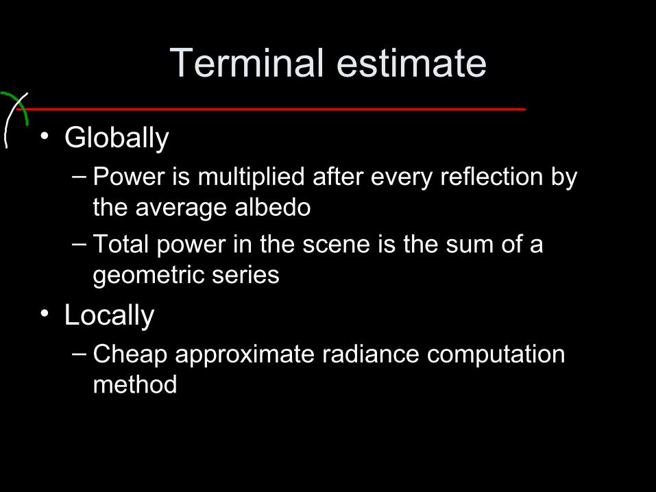
• Globally– Power is multiplied after every reflection by
the average albedo– Total power in the scene is the sum of a
geometric series
• Locally– Cheap approximate radiance computation
method

Results
Classic RR Improved RR
Up to 30% speedup

Local guess
• Finite element shooting walk algorithm– negligible time cost
Classic RR Improved RR Terminal guess

Example 2
Spectral optimisation
for path termination

Spectral optimisation
• Red light arrives on green wall
• Blue light arrives on yellow plastic with white specular– high diffuse albedo– no diffuse reflection
?high
albedo
?

Spectral optimisation
• Importance sampling– keep estimator value constant
Scalar value Vector value
a w
s = a s =
L Lw
L
L w
L La

Spectral optimisation
Classic Spectral optimisation

Example 3
”Go with the Winners” in Path Tracing

Path tracing with Russian-roulette
Problems:• Little reuse• Number of samples of n-bounce is proportional to the total contribution of n-bounce paths

Example: Russian roulette
mirror,albedo = 1
diffusealbedo = 0.25
env
env
env
2 rays
8 rays
Number of samples of n-bounce is proportional to the contribution of n-bounce paths
8 rays

Example: Go with the winners
mirror,albedo = 0.5
diffusealbedo = 0.25
1 ray1 ray
env
env
env16 rays
Number of samples of n-bounce is proportional to the variance of n-bounce paths

Random path continuation
Continuation with the probability of the albedo
Russian-roulette Go with the winners
Continuation
Termination
Splitting
Number of children isproportional to the anticipated error
fractional numberof children

Estimation of the anticipated error
env
env
envPotential of theprevious path segment
Albedo of the given point
Variance of the incoming radiance
Variance of the direction(scattering)
Variance of theradiance estimationat a given direction
+A
(s+1)2 B

Simulation results: Mona Lisa and a table
Russian roulette2 million rays, 19 seconds
Go with the winners2 million rays, 15 seconds

Simulation results:Mona Lisa and a table
Russian-roulette 10 million rays, 104 secs
Go with the winners10 million rays, 76 secs

Example 4
Improved Indirect Photon Mapping with
Weighted Importance Sampling

Weighted Importance Sampling
Integrand: f
Sampling density: p(x)
x
Targetdensity: g(x)
f(xi)/p(xi) M
Classical Monte Carlo Estimate:
f(xi)/p(xi) g(xi)/p(xi)
Weighted Monte Carlo Estimate:

Virtual light sources (instant radiosity, indirect photon mapping)

Radiance estimate for virtual light sources
High contribution sample generated with relatively low probability

Application of Weighted Importance Sampling
y
x
Target g: the probability density of path tracing

Original indirect photon mapping (no direct illumination)
With weighted importance sampling (no direct illumination)

Example 5
A Simple and Robust Mutation Strategy for the
Metropolis Light Transport

Metropolis Sampling
Integrand: f
1. Find I that mimics f
2. Find the normalization constant: b = I dx
Sampling: Mutation/Acceptance
- arbitrary mutation T(x y)- carefully selected acceptance probability a(x y)
Importance: I
a(x y)=I(x)·T(x y)
I(y)·T(y x)

Drawbacks of Metropolis
• Start-up bias– Process only converges to the stationary state
• Correlated samples– Increase the variance of the integral quadrature
• Number of samples in a pixel I– few samples for dark regions
Good mutation strategy
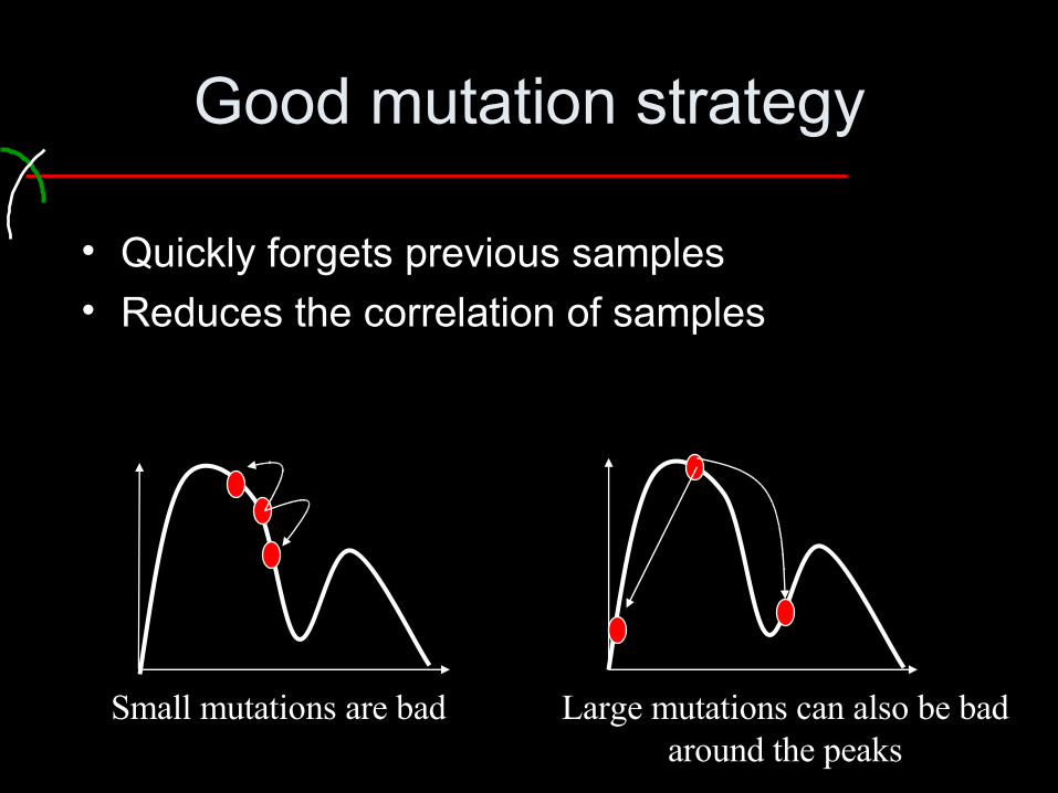
• Quickly forgets previous samples• Reduces the correlation of samples
Small mutations are bad Large mutations can also be badaround the peaks

Importance controlled mutation size
• Big mutations at unimportant regions and fine, small mutations at important regions
• Transform the domain to expand important regions and shrink unimportant regions and use uniform perturbations

Perturbing in the space of pseudo-random numbers
• Transformation for free: BRDF sampling, lightsource sampling, Russian Roulette
Primary sample space

Mutating in the Primary Sample Space
u1, u3
u2, u4 , u6, u8
u5u7, u9
u11
U=(u1 ,…)u10
u12, u14
u16
Path space Primary sample space

Mutating in the Primary Sample Space
U=(u1 ,…)
Path space Primary sample space

Ergodicity: Large (independent) Steps
Importance=0
1. Small steps with peturbation2. Large steps independently of the actual sample: plarge

Benefits of Large steps
• Ergodicity
• Sampling process forgets
• Reduces the start-up bias• Can be used to compute the normalization
constant b
• Sequence of large steps is a conventional random walk: Combination with Metropolis– multiple importance sampling

Implementation
primary samplespace of randomnumbers
path generation
adding the
contribution
randomnumber
generation
randomnumber
generation
adding the
contribution

Bidir path tracing Metropolis
25 samples per pixel

Effects of large step probability
plarge=0.02 plarge=0.5 plarge=0.9

Multiple Importance sampling
Mean value substitution Multiple Importance sampling

Example 6
Combined Correlated and
Importance Sampling
in Direct Illumintion Computation for Area Lights
and Environment Mapping

Correlated sampling
integrand fmain part g
+J = g dz
f dz =
g dz + f-g dz =
J + f-g dzI = f dz
f-g

Problem spots - example
direct lighting, area light source
could be calculated analytically
correlated sampling

Problem spots - example
direct lighting, area light source
could be calculated analytically
correlated sampling

Linear combination
f g g f 0
fp
fp
gpJ-
fp
gpJ-
f-gpJ g
f
correlated estimator importance estimator

Finding the
minimizing the variance:
~ correlation of f/p and g/p
provides the formula:
computed from the samples
only asymptotically unbiased
() = E2
f(z) p(z)
g(z) p(z) + J - p(z) p(z) - I
=E
Eg(z) p(z) J -
2
g(z) p(z) J -
f(z) p(z) I -

Light source sampling
occluderemittance Le
visibility vgeom factor G
BRDF fr
light
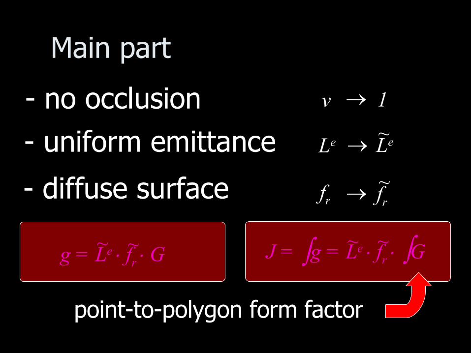
Main part
- uniform emittance- no occlusion
- diffuse surface
point-to-polygon form factor
g = Le fr G~ ~ J = g = Le fr G
~ ~
Le
v
fr fr
Le
1
~
~

calculation
using derived formula
= 1 if fully visible = 0 if fully occluded
fractionalvisibility

Results - images
importancesampling

Results - images
correlatedsampling

Results - images
combinedsampling

Environment mapping & skylight illumination
occluder
radiance Lenv
visibility v
scattering density w

Main part
no occlusion
smooth map non-specular
f = Lenv v w
g = Lenv w g = Lenv ad~
J = g = Lenv ad
ad = wLenv = Lenv
~
~

correlated
Environment mapping results
combined
importance(emittance)

correlated
Environment mapping results
importance (BRDF)
combined

Thank you