variants of sudoku as useful experimental designsssca.org.in/media/4bksinha.pdfvariants of sudoku as...

Variants of SuDoKu as Useful Experimental Designs

Jyotirmoy Sarkar

Department of Mathematical Sciences

Indiana University–Purdue University Indianapolis, USA

Bikas K Sinha

Ex-Faculty, Applied Statistics Division

Indian Statistical Institute, Kolkata, India

Abstract

SuDoKu is an interesting combinatorial structure embedded within a Latin Square Design.

It has gained popularity as a combinatorial puzzle as attested by many web sites. SuDoKu

as an experimental design was introduced first by Subramani and Ponnuswamy (2009), who

overlooked the fact that orthogonality of estimates was sacrificed. A corrected statistical

analysis is provided in Saba and Sinha (2014) along with the underlying ANOVA Table

for such designs based on SuDoKu and mutually orthogonal SuDoKu squares. Here, we

construct a special subclass of cylindrical-shift SuDoKu designs that allow restrictions on

combinations of certain factors, while simultaneously achieve greater orthogonality between

other factors. We present an outline of data analysis for such designs. Finally, we construct

mutually orthogonal cylindrical-shift SuDoKu squares.

Key Words and Phrases: ANOVA Models, CRD, RBD, LSD, Mutually Orthogonal

LSD, SuDoKu, Mutually Orthogonal SuDoKu, Cylindrical-shift SuDoKu, Mutually Ortho-

gonal Cylindrical-shift SuDoKu, Internal Blocking, Connected Design, Circulant Matrix

1. Introduction

The key reference to this article is Saba and Sinha [2014] wherein the basic properties of

a SuDoKu as an experimental design have been presented. We believe there is much more

into this fascinating combinatorial puzzle when viewed from an application perspective. We

discuss some such practical issues while proposing SuDoKus to serve as experimental designs.

It is well-known that LSDs and their generalizations based on mutually orthogonal Latin

squares (MOLS), viewed as experimental designs, go beyond the CRDs and RCBDs in simul-

taneously eliminating external sources of variation in the experimental units in an ANOVA

set-up. Likewise, SuDoKu squares and their generalizations [using mutually orthogonal Su-

Statistics and ApplicationsVolume 12, Nos. 1&2, 2014 (New Series), pp. 35-60

DoKu squares (MOSS)] as experimental designs, go one step beyond LSDs and their genera-

lizations, and provide an extra dimension of utility as experimental designs. Thus, SuDoKu

[abbreviated as SDK, pronounced as SuDoKu, not pronounced letter-by-letter] squares serve

as ‘extensions’ of Latin Square Designs [LSDs]. These are different from the usual Graeco

LSDs. The peculiarity of a SDK lies in the fact that in addition to incorporating variati-

ons due to Row, Column and Treatment components [as in an LSD], it also includes an

‘additional’ component of variation, referred to as ‘Internal Block Classification’ (IBC).

To set the tone of the discussion in this paper, we consider an LSD of order 9 and a related

agricultural experiment involving 9 Suppliers [S]—represented by the 9 rows of the Latin

Square, 9 Days [D]—represented by the 9 columns of the Latin Square, and 9 Machines

[M]—represented by the letter (or number) symbols in the Latin Square. We assume the

Machine effect contrasts to be the parameters of primary interest. Clearly, the LSD (which

requires 81 experimental units) does provide orthogonal estimation of the three components

of variation [each with 8 degrees of freedom (df)] and also of the experimental error [with 56

df].

Since a full set of 8 MOLS of order 9 exist, we can as well incorporate a few additional

components of variation, on top of those considered above. We may note in passing the

following well-known fact: Since the incidence matrices of all pairwise components of variation

are of the form J = ((1)), these components are simultaneously and orthogonally estimated.

This is precisely the structural beauty of an LSD or of a Graeco LSD. However, the point

to be noted is that we are also assuming additional experimental conditions, without even

realizing it! For instance, in addition to Suppliers and Days if we also have Operators to

handle the Machines along with possible operator-to-operator variation, we do require the

availability of all operators on all days for a Graeco LSD to be implementable. In this case,

we have orthogonal estimation of all four components of variation [each with 8 degrees of

freedom (df)] and of the experimental error [with 48 df].

What if the operators are available only on a subset of days? Of course, we would like each

one of them to handle each of the 9 machines in some way or another so that Machine-to-

Machine variation can be estimated with maximum precision. A SDK, as an experimental

design, provides a combinatorial solution to the above problem when the operators are

believed to be available in teams of 3 on 3 consecutive days. Example 1 shows a popular

SDK of order 9.

36 JYOTIRMOY SARKAR ET AL. [Vol. 12, Nos. 1&2

Example 1: A SDK of order 9

S\D D1 D2 D3 D4 D5 D6 D7 D8 D9

S1 M1 M4 M7 M6 M2 M5 M9 M8 M3

S2 M9 M5 M8 M1 M7 M3 M4 M6 M2

S3 M2 M6 M3 M8 M9 M4 M5 M7 M1

Op1 Op4 Op7

S4 M6 M9 M5 M2 M4 M8 M3 M1 M7

S5 M7 M1 M4 M9 M3 M6 M2 M5 M8

S6 M3 M8 M2 M5 M1 M7 M6 M4 M9

Op2 Op5 Op8

S7 M5 M3 M1 M7 M6 M9 M8 M2 M4

S8 M4 M2 M6 M3 M8 M1 M7 M9 M5

S9 M8 M7 M9 M4 M5 M2 M1 M3 M6

Op3 Op6 Op9

Speculative sight of the SDK in Example 1 reveals that the Operators 1, 2, 3 are believed

to be available on Days 1, 2, 3; likewise, Operators 4, 5, 6 are available on Days 4, 5, 6; and

similarly Operators 7, 8, 9 are available on Days 7, 8, 9. Let us designate this specific type

of operator availability as ‘Scenario (1)’. When this obtains, the SDK can be viewed as

an ‘extension’ of the LSD and it entails orthogonal estimation of the Machine-to-Machine

variations with full 8 df—in spite of the restricted availability of the 9 operators! See Saba

and Sinha [2014] for technical details of the data analysis in a very general set-up for a SDK

of order n = pq with as many ‘internal blocks’ of size p × q, under Scenario (1). It may be

noted that in a SDK design, Machines are orthogonal to Rows, Columns and also Operators.

Therein lies the combinatorial beauty of a SDK design!

In contrast to the above scenario, we will discuss below some other meaningful alternative

scenarios.

2. Operator availability: Different constraints

We propose to study variations of the typical SDK design of order 9 to meet the demands

of practical situations to accommodate various forms of operator availability, and also to

provide a comprehensive analysis of the underlying data under such availability constraints.

We start by noting that in a usual SDK of order 9, the df attributed to Machines is 8,

whereas the df attributed to Rows [Suppliers] as well as to Columns [Days] are precisely 6

for pure contrasts and 2 for those contrasts that are ‘confounded’ with the Internal Blocks

[Operators]. Also, the df attributed to Internal Blocks [Operators] is 4 for pure contrasts,

derived through considerations of tetra differences, and the remaining 4 df are confounded

with rows and columns, each with 2 df. The error df is (81−1)− (8+6+2+6+2+4) = 52.

2014] VARIANTS OF SUDOKU AS USEFUL EXPERIMENTAL DESIGNS 37

See Saba and Sinha [2014] for details.

We ask if we could make available a special type of SDK with orthogonal estimation of one of

the two components—Row or Column—in addition to the Machine component, even when

there is a constraint on the operators’ availability? [Note that orthogonal estimation of all

three components amounts to using two Graeco Latin Squares of order 9 with unconstrained

availability of all operators.] The answer to the restricted set-up is in the affirmative for the

same constraint as mentioned above in Section 1 under Scenario (1). Below we display one

such SDK design in Example 2.

Example 2: A SDK design of order 9 with orthogonal estimation of row (supplier) and machine effects

and with operator availability as in Scenario (1)

S\D D1 D2 D3 D4 D5 D6 D7 D8 D9

S1 M1, O1 M2, O2 M3, O3 M4, O4 M5, O5 M6.O6 M7, O7 M8, O8 M9, O9

S2 M4, O1 M5, O2 M6, O3 M7, O4 M8, O5 M9, O6 M1, O7 M2, O8 M3, O9

S3 M7, O1 M8, O2 M9, O3 M1, O4 M2, O5 M3.O6 M4, O7 M5, O8 M6, O9







Example 2 affords orthogonal estimation of Row contrasts; that is, none of the row contrasts

is confounded with internal blocks (operators). Therefore, in the ANOVA Table, SS due

to Machines and Rows each carries 8 df, whereas SS due to Columns has 6 pure df and

2 df confounded with Operators. Operator SS will have 6 pure df in this case (with 2 df

confounded with columns). Henceforth, we will use Rows and Suppliers (and also Columns

and Days) interchangeably. The error df is (81− 1)− (8 + 8 + 6 + 2 + 6) = 50.

Example 2 shows operator assignments when teams of 3 operators are available on non-

overlapping clusters of 3 consecutive days, i.e., under Scenario (1). Clearly, both Operator

and Machine assignments have been spread across all the 9 Suppliers to provide orthogonal

estimation of Row contrasts.

Next, we propose to discuss some other scenarios of availability of the 9 operators in the

above framework of an experimental design:

Scenario (2): Operator i is available on consecutive Days i, i+1, i+2 (modulo 9); 1 ≤ i ≤ 9;

Scenario (3): Operator i is available on alternate Days i, i+ 2, i+ 4 (modulo 9); 1 ≤ i ≤ 9.


Scenario (2): First note that in the usual SDK of order 9 [Example 1 above], we must ‘right-

shift’ Operator 2 by a day in order to accommodate her availability on Days 2, 3, 4 (still letting

her work with Suppliers 4, 5, 6). But this implies that Operator 2 would work on different ma-

chines with unequal frequencies given by Machine(frequency): 1(1), 2(2), 4(1), 5(2), 8(1), 9(2).

More specifically, Operator 2 would totally skip Machines 3, 6, 7; while she would work once

on Machines 1, 4, 7 and twice on Machines 2, 5, 9. Consequently, it would not be possible to

estimate Machine effects orthogonally to Operator effects.

In order to avoid this situation, we need a special type of SDK which will satisfy the above

requirement on the availability of Operators and at the same time allow orthogonal estimati-

on of all Machine effect contrasts. Indeed such a SDK exists, and it is displayed in Example 3

below. This is how it is constructed: First, superimpose the operator assignment of Exam-

ple 1 on to the machine allocation of Example 2. Next, keep Operators 1, 4, 7 unchanged,

but shift Operators 2, 5, 8 by a day (with the understanding that Operator 8 is assigned to

work on Days 8, 9, 1), and shift Operators 3, 6, 9 by two days (so that Operator 9 works on

Days 9, 1, 2).

Example 3: A SDK of order 9, when operators are available on consecutive days

S\D D1 D2 D3 D4 D5 D6 D7 D8 D9

S1 M1, O1 M2, O1 M3, O1 | M4, O4 M5, O4 M6, O4 | M7, O7 M8, O7 M9, O7 |S2 M4, O1 M5, O1 M6, O1 | M7, O4 M8, O4 M9, O4 | M1, O7 M2, O7 M3, O7 |S3 M7, O1 M8, O1 M9, O1 | M1, O4 M2, O4 M3, O4 | M4, O7 M5, O7 M6, O7 |S4 M2, O8 | M3, O2 M1, O2 M5, O2 | M6, O5 M4, O5 M8, O5 | M9, O8 M7, O8

S5 M5, O8 | M6, O2 M4, O2 M8, O2 | M9, O5 M7, O5 M2, O5 | M3, O8 M1, O8

S6 M8, O8 | M9, O2 M7, O2 M2, O2 | M3, O5 M1, O5 M5, O5 | M6, O8 M4, O8

S7 M3, O9 M1, O9 | M2, O3 M6, O3 M4, O3 | M5, O6 M9, O6 M7, O6 | M8, O9



We call the SDK in Example 3 a ‘cylindrical-shift SDK’ (CSDK) of order 9 (this name will

be made clearer in Section 3). The use of this CSDK as an experimental design provides

orthogonal estimation of all Machine effects. See Appendix A for an outline of analysis for

this CSDK design.

What about estimation of Row/Column/Operator effects? In Example 3, operator effect is

not orthogonal to either row or column. Is it possible to satisfy the above requirements on the

operators’ availability and at the same time provide orthogonal estimation of Operator and

one other effect [Row/Column]? The answer is in the affirmative, and we get an ‘improved’

operator assignment displayed in Example 4 below. We will explain in Section 4 how we

obtain the CSDK of Example 4.


Example 4: A cylindrical-shift SDK of order 9, when operators are available on consecutive days,

making operator orthogonal to supplier

S\D D1 D2 D3 D4 D5 D6 D7 D8 D9

S1 M1, O1 M2, O2 M3, O3 M4, O4 M5, O5 M6, O6 M7, O7 M8, O8 M9, O9 |S2 M4, O1 M5, O2 M6, O3 M7, O4 M8, O5 M9, O6 M1, O7 M2, O8 M3, O9 |S3 M7, O1 M8, O2 M9, O3 M1, O4 M2, O5 M3, O6 M4, O7 M5, O8 M6, O9 |S4 M2, O9 | M3, O1 M1, O2 M5, O3 M6, O4 M4, O5 M8, O6 M9, O7 M7, O8

S5 M5, O9 | M6, O1 M4, O2 M8, O3 M9, O4 M7, O5 M2, O6 M3, O7 M1, O8

S6 M8, O9 | M9, O1 M7, O2 M2, O3 M3, O4 M1, O5 M5, O6 M6, O7 M4, O8

S7 M3, O8 M1, O9 | M2, O1 M6, O2 M4, O3 M5, O4 M9, O5 M7, O6 M8, O7



Naturally, for the CSDK of Example 4 with this improved operator assignment, the SS for

Machines and Rows are still orthogonal, each with 8 df. As in Example 3, Machines and Co-

lumns are still orthogonal. But now, Operators and Rows are also orthogonal. What about

Operators and Columns? In Appendix A, we provide the analysis of this non-orthogonal, but

connected operator-day design—viewed as a block design! We discuss more about connec-

tedness in Appendix B.

Remark 1. Note that Examples 3 and 4 are derived from the ‘key’ SDK in Example 2

simply by proper placement of the operators across the row-column combinations. We

believe very few SDK’s are amenable to this kind of cylindrical-shift property. Surely,

the SDK in Example 1 fails to preserve any such property.

Scenario (3): Here we want to accommodate ‘alternate day availability’ of each operator

(modulo 9). In Example 5 below we provide a CSDK square of order 9 with the following

two properties: (i) Operator availability on alternative days, and (ii) Row effects are still

orthogonal to Operators. In fact, the Machine allocation in Example 5 is exactly the same

as in Examples 2, 3, 4. Again, in Appendix A, we provide the analysis of this design.

Example 5: A cylindrical-shift SDK of Order 9 when operators are available on alternate days,

making operator orthogonal to supplier

S\D D1 D2 D3 D4 D5 D6 D7 D8 D9

S1 M1, O1 M2, O2 M3, O3 M4, O4 M5, O5 M6, O6 M7, O7 M8, O8 M9, O9 |S2 M4, O1 M5, O2 M6, O3 M7, O4 M8, O5 M9, O6 M1, O7 M2, O8 M3, O9 |S3 M7, O1 M8, O2 M9, O3 M1, O4 M2, O5 M3, O6 M4, O7 M5, O8 M6, O9 |S4 M2, O6 M3, O7 M1, O8 M5, O9 | M6, O1 M4, O2 M8, O3 M9, O4 M7, O5

S5 M5, O6 M6, O7 M4, O8 M8, O9 | M9, O1 M7, O2 M2, O3 M3, O4 M1, O5

S6 M8, O6 M9, O7 M7, O8 M2, O9 | M3, O1 M1, O2 M5, O3 M6, O4 M4, O5





3. CSDK of order 15 = 5× 3 with operator availability constraints

A SDK of order 15 is not hard to find or construct. See Example 6 below. With a 5 × 3

internal block classification, it provides a solution to an experimental scenario involving 15

rows [Suppliers], 15 columns [Days], 15 treatments [Machines] and 15 Operators—with the

stipulation that 3 operators are available in each of the five non-overlapping clusters of 3

consecutive days; namely, Days 1–3, 4–6, 7–9, 10–12, 13–15. In this SDK, viewed as an

experimental design, Machines are orthogonal to all other classifications. But Operators are

confounded with Suppliers [2 df] and Days [4 df], and we have only 8 df available for ‘pure’

operator effects. Suppliers account for 12 df on pure SS and 2 df on SS confounded with the

Operators. Days account for 10 df on pure SS and the remaining 4 df on SS confounded with

the Operators. The error df is (152−1)− (14+12+2+10+4+8) = 174. That is the typical

scenario if one starts with an arbitrary SDK of order 15.

Example 6: A SDK of Order 15

S\D D1 D2 D3 D4 D5 D6 D7 D8 D9 D10 D11 D12 D13 D14 D15

S1 2 9 15 11 13 4 1 14 12 8 3 10 5 6 7

S2 10 14 4 1 7 5 8 2 9 11 13 6 12 3 15

S3 1 12 11 9 2 3 6 10 7 14 15 5 8 4 13

S4 13 6 5 10 8 14 3 4 15 1 7 12 9 11 2

S5 7 3 8 15 12 6 13 11 5 9 4 2 1 14 10

Op1 Op4 Op7 Op10 Op13

S6 8 11 14 12 10 15 4 7 6 2 5 1 13 9 3

S7 15 2 6 13 1 11 9 3 10 12 8 4 7 5 14

S8 4 13 10 5 6 9 2 1 11 7 14 3 15 12 8

S9 9 5 12 7 3 2 15 8 14 13 10 11 4 1 6

S10 3 1 7 4 14 8 5 12 13 6 9 15 2 10 11


S11 6 10 2 3 11 13 7 15 1 4 12 9 14 8 5

S12 11 7 9 14 5 1 12 13 2 10 6 8 3 15 4

S13 12 4 3 2 15 7 11 6 8 5 1 14 10 13 9

S14 5 8 1 6 4 10 14 9 3 15 2 13 11 7 12

S15 14 15 13 8 9 12 10 5 4 3 11 7 6 2 1


We ask whether it is possible to construct a SDK of order 15 with the property that Operator

is orthogonal to Supplier, even though Operators have restricted availability as in Scenario

(1): Operators 1–3 available on Days 1–3, Operators 4–6 available on Days 4–6, etc. Below

we show the (machine, operator) combination in each (supplier, day) combination, so that

Operator is orthogonal to Supplier (Row). The affirmative answer is given in Examples 7

below.


Example 7: A CSDK design of Order 15 showing (machine, operator) assignment within (supplier, day) combination

with Operator orthogonal to Supplier, when teams of 3 operators are available on clusters of 3 days


S1 1, 1 2, 2 3, 3 4, 4 5, 5 6, 6 7, 6 8, 8 9, 9 10, 10 11, 11 12, 12 13, 13 14, 14 15, 15

S2 4, 1 5, 2 6, 3 7, 4 8, 5 9, 6 10, 6 11, 8 12, 9 13, 10 14, 11 15, 12 1, 13 2, 14 3, 15

S3 7, 1 8, 2 9, 3 10, 4 11, 5 12, 6 13, 6 14, 8 15, 9 1, 10 2, 11 3, 12 13, 13 14, 14 15, 15

S4 10, 1 11, 2 12, 3 13, 4 14, 5 15, 6 1, 6 2, 8 3, 9 4, 10 5, 11 6, 12 7, 13 8, 14 9, 15

S5 13, 1 14, 2 15, 3 1, 4 2, 5 3, 6 4, 6 5, 8 6, 9 7, 10 8, 11 9, 12 10, 13 11, 14 12, 15

S6 2, 3 3, 1 1, 2 5, 6 6, 4 4, 5 8, 9 9, 7 7, 8 11, 12 12, 10 10, 11 14, 15 15, 13 13, 14

S7 5, 3 6, 1 4, 2 8, 6 9, 4 7, 5 11, 9 12, 7 10, 8 14, 12 15, 10 13, 11 2, 15 3, 13 1, 14

S8 8, 3 9, 1 7, 2 11, 6 12, 4 10, 5 14, 9 15, 7 13, 8 2, 12 3, 10 1, 11 5, 15 6, 13 4, 14

S9 11, 3 12, 1 10, 2 14, 6 15, 4 13, 5 2, 9 3, 7 1, 8 5, 12 6, 10 4, 11 8, 15 9, 13 7, 14

S10 14, 3 15, 1 13, 2 2, 6 3, 4 1, 5 5, 9 6, 7 4, 8 8, 12 9, 10 7, 11 11, 15 12, 13 10, 14

S11 3, 2 1, 3 2, 1 6, 5 4, 6 5, 4 9, 8 7, 9 8, 7 12, 11 10, 12 11, 10 15, 14 13, 15 14, 13

S12 6, 2 4, 3 5, 1 9, 5 7, 6 8, 4 12, 8 10, 9 11, 7 15, 11 13, 12 14, 10 3, 14 1, 15 2, 13

S13 9, 2 7, 3 8, 1 12, 5 10, 6 11, 4 15, 8 13, 9 14, 7 3, 11 1, 12 2, 10 6, 14 4, 15 5, 13

S14 12, 2 10, 3 11, 1 15, 5 13, 6 14, 4 3, 8 1, 9 2, 7 6, 11 4, 12 5, 10 9, 14 7, 15 8, 13

S15 15, 2 13, 3 14, 1 3, 5 1, 6 2, 4 6, 8 4, 9 5, 7 9, 11 7, 12 8, 10 12, 14 10, 15 11, 13

Note that the machine allocation matrix (ignoring the operator assignment) has the following

‘cylindrical-shift’ property: Fold the machine allocation SDK square so that the left edge and

the right edge are joined together to form a (vertical) cylinder. Cut this cylinder into q equal

small (vertical) cylinders consisting of p contiguous rows each. Then any contiguous p × q

sub-matrix on any small (vertical) cylinder contains all machines exactly once! We call such

a machine allocation matrix a cylindrical-shift SuDoKu (CSDK) square.

Let us illustrate the cylindrical-shift property of machine allocation in Example 7. Consider

only the last p = 5 contiguous rows in Example 7. Then any three contiguous columns in this

portion of the machine allocation matrix, such as columns (1, 2, 3), (2, 3, 4), . . . , (14, 15, 1),

(15, 1, 2), contain all machines exactly once! A few such contiguous columns are shown below,

Example 7 (continued): Illustrating the cylindrical-shift property of machine allocation:

For instance, Columns (5, 6, 7), (9, 10, 11), (14, 15, 1) contain all machines exactly once


S11 3 1 2 6 4 5 9 7 8 12 10 11 15 13 14

S12 6 4 5 9 7 8 12 10 11 15 13 14 3 1 2

S13 9 7 8 12 10 11 15 13 14 3 1 2 6 4 5

S14 12 10 11 15 13 14 3 1 2 6 4 5 9 7 8

S15 15 13 14 3 1 2 6 4 5 9 7 8 12 10 11

(Columns 5, 6, 7) (Columns 9 , 10 , 11 )

In fact, a similar horizontal cylindrical-shift property exists if we fold the machine allocation

SDK square so that the top edge and the bottom edge are joined together to form a horizontal


cylinder, and then cut this cylinder into p equal small horizontal cylinders consisting of q

contiguous columns each. In this case, any contiguous p×q sub-matrix on any small horizontal

cylinder contains all machines exactly once! As marvelous as this horizontal cylindrical-shift

property is, we will only utilize the vertical cylindrical-shift property for operator allocation.

This CSDK square (of machine allocation) is within the framework of the above availability

constraints of the Operators, and yet Operator assignment can be made orthogonal to Sup-

plier classification. When in a CSDK square such an operator assignment is made orthogonal

to suppliers we call it a CSDK design. Naturally, this is more desirable; and we can work

out a joint analysis of Days versus Operators in the standard format of a block design as

was done for the case of CSDK design of order 9.

In the layout of Example 7, Operators 1–3 are available together as a team on a cluster of

Days 1–3, etc. Consequently, Days and Operators are confounded and the resulting design is

disconnected (for example, an elementary contrast between effects of Operators in different

teams is not estimable). Can we develop a Operator-Day connected design (that is, all

operator contrasts are estimable) preserving Operator-Supplier orthogonality? Towards this,

we consider two scenarios of operator availability across days, as were presented above.

Scenario (2): Operator i is available on consecutive Days i, i+1, i+2 (modulo 15); 1 ≤ i ≤ 15;

Scenario (3): Operator i is available on alternate Days i, i+2, i+4 (modulo 15); 1 ≤ i ≤ 15.

To save space we present below only Rows 1, 6, 11 of the CSDK design. The rest of the rows

are developed as in Example 7. That is, in the k-th row (k = 1, 2, 3, 4) after a displayed row,

the label of the machine is 3k larger than the label of the machine in the given row (modulo

15), while the operator is the same as the operator in the given row.

Example 8: A CSDK of Order 15 showing (machine, operator) allocation for Supplier Groups 1(S1–S5), 2(S6–S10), 3(S11–S15)

with Operator orthogonal to Supplier, when operators are available on ‘consecutive days’ per Scenario (2)

G\D D1 D2 D3 D4 D5 D6 D7 D8 D9 D10 D11 D12 D13 D14 D15

G1 1, 1 2, 2 3, 3 4, 4 5, 5 6, 6 7, 6 8, 8 9, 9 10, 10 11, 11 12, 12 13, 13 14, 14 15, 15

G2 2, 15 3, 1 1, 2 5, 3 6, 4 4, 5 8, 6 9, 7 7, 8 11, 9 12, 10 10, 11 14, 12 15, 13 13, 14

G3 3, 14 1, 15 2, 1 6, 2 4, 3 5, 4 9, 5 7, 6 8, 7 12, 8 10, 9 11, 10 15, 11 13, 12 14, 13


Example 9: A CSDK of Order 15 showing (machine, operator) for Suppliers Groups 1(S1–S5), 2(S6–S10), 3(S11–S15)

with Operator orthogonal to Supplier, when operators are available on ‘alternate days’ per Scenario (3)

G\D D1 D2 D3 D4 D5 D6 D7 D8 D9 D10 D11 D12 D13 D14 D15

G1 1, 1 2, 2 3, 3 4, 4 5, 5 6, 6 7, 6 8, 8 9, 9 10, 10 11, 11 12, 12 13, 13 14, 14 15, 15

G2 14, 12 15, 13 13, 14 2, 15 3, 1 1, 2 5, 3 6, 4 4, 5 8, 6 9, 7 7, 8 11, 9 12, 10 10, 11

G3 3, 14 1, 15 2, 1 6, 2 4, 3 5, 4 9, 5 7, 6 8, 7 12, 8 10, 9 11, 10 15, 11 13, 12 14, 13

4. CSDK design of order n = p× q with operator availability constraints

We describe here the construction of a CSDK design of order n = pq with internal blocks of

size p × q. We exhibit the machine allocation within each (supplier, day) combination, and

also the operator assignment which accommodates their availability constraints.

We desire the following features of the design: (1) Operator versus Supplier [Row] orthogo-

nality, (2) Operator versus Days [Columns] connectedness, and (3) all three factors [Opera-

tors/Suppliers/Days] orthogonal to Machines [Treatments]. As we noted in the two earlier

sections, an arbitrary SDK fails to achieve these properties. We will choose a CSDK square

and assign operators carefully to construct a CSDK design that attains the above features.

We assume that q ≥ 3, q ̸= 6. For such a q, it is well known [see Bose, Srikhande and Parker

(1960)] that there exists a pair of orthogonal Latin Squares (Lq0, L

q1) of order q. Of course, a

Latin Square Mp1 of order p always exists.

We write down the machine numbers in a p×q rectangular array K in the natural order row-

by-row. That is, the rows of K are: K1∗ = (1, 2, . . . , q);K2∗ = (q+1, q+2, . . . , 2q); . . . ;Kp∗ =

((p − 1)q + 1, (p − 1)q + 2, . . . , pq = n). Next, we write down the Latin square Mp1 using

symbols {1, 2, . . . , p} in standard form (that is, the symbols are in the natural order in the

first row). Now replace each symbol i by the row vector Ki∗ = ((i−1)q+1, (i−1)q+2 . . . , iq),

to construct a p × qp = n array of numbers A, say. Note that the top row of A consists of

numbers 1, 2, 3, . . . , n in the natural order. Let A∗1, A∗2, . . . , A∗n denote the columns of A.

Next, we write down the Latin square Lq1 using symbols {1, 2, . . . , q} in standard form;

then we concatenate to its right the same Latin square Lq1, but written using symbols

{q + 1, q + 2, . . . , 2q} in standard form; and so on until we concatenate the p-th copy of the

same Latin square Lq1 written using symbols {(p− 1)q+1, (p− 1)q+2, . . . , pq} in standard

form. Thus we have a q× pq = q× n array of symbols {1, 2, . . . , n}. Finally, we replace eachsymbol j by the entire column A∗j, for 1 ≤ j ≤ n to obtain an n×n array V showing machine


allocation in each cell (that is, in each combination of supplier (row) and day (column)). In

Theorem 1, we establish that V is a CSDK square.

Theorem 1 The array V obtained as above usingK,Mp1 , L

q1 is a CSDK square using symbols

{1, 2, 3, . . . , n}.

Proof. First note that since each row of Mp1 contains all symbols 1, 2, . . . , p, each row of

A is a concatenation of some permutation of all rows of K, and hence a permutation of all

symbols {1, 2, 3, . . . , n}. Next, note that no two rows of A have any matching symbol since

all symbols within each column of A are different. Also, note that A is a 1× p block matrix

with the j-th block given by a permutation of all p rows of K according to the j-th column

of Latin square Mp1 . Hence, each of the p blocks of A consists of all symbols {1, 2, 3, . . . , n}

in K.

Next, note that V is a q×p block matrix with top row of this block matrix given by A, and the

(k, l)-th block of V is given by a permutation of columns in the (1, l)-th block of V for every

k ≤ q and every l ≤ p. This ensures all rows of V are permutations of {1, 2, 3, . . . , n}, notwo rows within the k-th row-block of V have any matching symbol, and all blocks consist of

symbols {1, 2, 3, . . . , n}. Also, since Lq1 is a Latin square, no two rows in different row-blocks

k, k′ have any matching element, and all columns of V are permutations of {1, 2, 3, . . . , n}.Thus, V is a SDK square.

The (vertical) cylindrical-shift property of V follows from the fact that the rows of K are

identical (modulo q). Hence, V is a CSDK square. Q.E.D.

To complete the CSDK design it now remains to prescribe the operator assignment in each

cell according as their availability in three different scenarios: (1) A team of q operators are

available in each non-overlapping set of q days, (2) Operator i is available on q consecutive

days (i, i+1, . . . , i+ q− 1) (modulo n); and (3) Operator i is available on days (i, i+ d1, i+

d2, . . . , i+ dq−1) (modulo n). We refer to such operator assignment in Scenario (3) as design

d = (0, d1, d2, . . . , dq−1). Note that Scenario (2) is a special case of Scenario (3) in which

dk = k, or d = (0, 1, 2, . . . , q − 1). Also note that design d = (0, p, 2p, . . . , (q − 1)p) in

Scenario (3) reduces to Scenario (1) if we renumber the days and the operators in design d

as follows:

1 p+ 1 . . . (q − 1)p+ 1

2 p+ 2 . . . (q − 1)p+ 2

· · · · · · · · · · · ·p 2p . . . qp

−→

1 2 . . . q

q + 1 q + 2 . . . 2q

· · · · · · · · · · · ·(p− 1)q + 1 (p− 1)q + 2 . . . qp


Of course, in Scenario (1), one operator is assigned in each internal block, which causes

operator-supplier non-orthogonality. In Scenarios (2) and (3) in order to achieve operator-

supplier orthogonality, we shall further assume that design d is such that {0, d1, d2, . . . , dq−1}are distinct modulo q. This condition certainly holds true in Scenario (2). [When this con-

dition is violated, operator assignment becomes more complicated. We will not address the

operator allocation in such a case, except to give an illustration in (3b) of Example 10 below.]

We write down the Latin square Lq0, which is orthogonal to the Latin square Lq

1, using symbols

{1, 2, . . . , q} in standard form. We concatenate p identical copies of this q × q array Lq0 to

obtain a q×qp = q×n array B = (bhi), say, written using symbols {1, 2, . . . , q}. For each i ≤n, identify the columns corresponding to the days when operator i is available according to

the different scenarios, and replace the symbol b1i in these q identified columns by operator

i. Since {0, d1, d2, . . . , dq−1} are distinct modulo q, operator i appears in q different rows (and

will not be changed again as the operator assignment continues), ensuring orthogonality with

supplier (row). This transforms the array B into a new q × n array D, say, using symbols

{1, 2, . . . , n}. Finally, replace each symbol j in D by a column vector consisting of p copies

of j, to obtain a n× n array W , say. Finally, we superimpose W on the CSDK square V of

order n to complete the CSDK design (V,W ).

Remark 2. The operator assignment is the same for all suppliers within the same group,

where Group 1 consisting of suppliers (1, 2, . . . p), Group 2 of (p + 1, . . . , 2p), etc. up

to Group q consisting of suppliers ((q − 1)p+ 1, . . . , qp).

Remark 3. The operator assignment can vary according as the operators’ availability, wi-

thout changing the machine allocation.

Remark 4. In Appendix B we discuss the operator-day connectedness for the CSDK design

(V,W ); that is, for any two operators there is a chain of operators such that each pair

of successive operators work together on the same day. In particular, the design is

connected in Scenario (2), but disconnected in Scenario (1).

Below we present, as illustration, the R codes needed to construct a CSDK design of order

12 = 3 × 4, followed by the design these codes produced in Example 10. CSDK designs

of other orders can be obtained by modifying these codes suitably. Examples (2, 4, 5) of

Section 2 and Examples (7, 8, 9) of Section 3 showed CSDK designs of order 9 = 3× 3 and

15 = 5× 3 respectively. Section 5 shows CSDK designs of order 16 = 4× 4 in Examples (11,

11B), and of order 20 = 4×5 in Example 12, if attention is restricted to only one of machine,

feature or characteristic allocation.


R codes used to generate CSDK design of order 12 = 3× 4

(available at www.math.iupui.edu/~jsarkar/Rcodes/Sudoku.R)

p=3; q=4; n=p*q; # Enter p and q, and calculate n

# Write 1:n in a pxq array in natural order row-by-row

K=matrix(1:n, c(p,q), byrow=TRUE)

# Enter (orthogonal) Latin square(s) of order p

M1=matrix(c(1,2,3, 2,3,1, 3,1,2), c(p,p), byrow=TRUE)

# Define machine groups as columns of A

A=matrix( as.vector(t(K[as.vector(t(M1)),])), c(p,n), byrow=TRUE)

# Enter orthogonal Latin squares of order q

L0=matrix(c(1,2,3,4, 2,1,4,3, 3,4,1,2, 4,3,2,1), c(q,q), byrow=TRUE)

L1=matrix(c(1,2,3,4, 3,4,1,2, 4,3,2,1, 2,1,4,3), c(q,q), byrow=TRUE)

# Determine machine allocation

Machine=cbind(

matrix(c(A[,as.vector(L1 )]), c(n,q)),

matrix(c(A[,as.vector(L1+q )]), c(n,q)),

matrix(c(A[,as.vector(L1+2*q)]), c(n,q)) )

# Operator assignments

# Scenario (1): Teams of q operators available in blocks of q days

Operator=cbind(L0, L0+q, L0+2*q) # p copies of L0 on different symbols

# Scenarios (2), (3): Operator i works on days d=(i, i+d_1, ..., i+d_{q-1})

Op=cbind(L0, L0, L0) # start with p copies of L0, and modify

d=c(0,1,2,3) # spacing of work days for operators in Scenario (2)

d=c(0,2,5,7) # spacing of work days for operators in Scenario (3)

for (i in 1:n){ a=Op[1,i]; id=i+d

for (l in 1:q){ if(id[l]>n){id[l]=id[l]-n} }

for (j in id){ for (k in 1:q){if(Op[k,j]==a){Op[k,j]=i}} }

}

Op # operator assignments for groups of p suppliers

Operator=matrix(rep(as.vector(Op), each=p), c(n,n) )

Machine; Operator # print machine allocation and operator assignment

The CSDK design of order 12 = 3× 4 showing machine allocation and operator assignment

in all three scenarios against each (supplier, day) combination is displayed next.


Example 10: A CSDK design of order 12 = 3× 4 showing machine allocation and operator assignment in several scenarios

Machine

| D1 D2 D3 D4 | D5 D6 D7 D8 | D9 D10 D11 D12

-------|------------------------------------------------------------------

S1 | 1 2 3 4 | 5 6 7 8 | 9 10 11 12

S2 | 5 6 7 8 | 9 10 11 12 | 1 2 3 4

S3 | 9 10 11 12 | 1 2 3 4 | 5 6 7 8

-------|------------------------------------------------------------------

S4 | 3 4 1 2 | 7 8 5 6 | 11 12 9 10

S5 | 7 8 5 6 | 11 12 9 10 | 3 4 1 2

S6 | 11 12 9 10 | 3 4 1 2 | 7 8 5 6

-------|------------------------------------------------------------------

S7 | 4 3 2 1 | 8 7 6 5 | 12 11 10 9

S8 | 8 7 6 5 | 12 11 10 9 | 4 3 2 1

S9 | 12 11 10 9 | 4 3 2 1 | 8 7 6 5

-------|------------------------------------------------------------------

S10 | 2 1 4 3 | 6 5 8 7 | 10 9 12 11

S11 | 6 5 8 7 | 10 9 12 11 | 2 1 4 3

S12 | 10 9 12 11 | 2 1 4 3 | 6 5 8 7

(1) Operator (Teams of 4 operators available in clusters of 4 days )

| D1 D2 D3 D4 | D5 D6 D7 D8 | D9 D10 D11 D12

-------|------------------------------------------------------------------

S1-S3 | 1 2 3 4 | 5 6 7 8 | 9 10 11 12

S4-S6 | 2 1 4 3 | 6 5 8 7 | 10 9 12 11

S7-S9 | 3 4 1 2 | 7 8 5 6 | 11 12 9 10

S10-S12| 4 3 2 1 | 8 7 6 5 | 12 11 10 9

(2) Operator (Operator i available on Days {i, i+1, i+2, i+3} (modulo 12) )

| D1 D2 D3 D4 | D5 D6 D7 D8 | D9 D10 D11 D12

-------|------------------------------------------------------------------

S1-S3 | 1 2 3 4 | 5 6 7 8 | 9 10 11 12

S4-S6 | 10 1 12 3 | 2 5 4 7 | 6 9 8 11

S7-S9 | 11 12 1 2 | 3 4 5 6 | 7 8 9 10

S10-S12| 12 11 2 1 | 4 3 6 5 | 8 7 10 9

(3a) Operator (Operator i available on Days {i, i+2, i+5, i+7} (modulo 12) )

| D1 D2 D3 D4 | D5 D6 D7 D8 | D9 D10 D11 D12

-------|------------------------------------------------------------------

S1-S3 | 1 2 3 4 | 5 6 7 8 | 9 10 11 12

S4-S6 | 6 9 8 11 | 10 1 12 3 | 2 5 4 7

S7-S9 | 11 12 1 2 | 3 4 5 6 | 7 8 9 10

S10-S12| 8 7 10 9 | 12 11 2 1 | 4 3 6 5

(3b) Operator (Operator i available on Days {i, i+2, i+4, i+6} (modulo 12) )

In this case {0, 2, 4, 6} are not distinct (modulo 4). So, the operator

assignment algorithm is modified (details omitted).

| D1 D2 D3 D4 | D5 D6 D7 D8 | D9 D10 D11 D12

-------|------------------------------------------------------------------

S1-S3 | 1 2 3 4 | 5 6 7 8 | 9 10 11 12

S4-S6 | 9 10 11 12 | 1 2 3 4 | 5 6 7 8

S7-S9 | 11 12 1 2 | 3 4 5 6 | 7 8 9 10

S10-S12| 7 8 9 10 | 11 12 1 2 | 3 4 5 6


Note that the operator-day design is disconnected in Scenario (1), but connected in Scenarios

(2) and (3a). The design is disconnected in Scenario (3b) because operators with odd serial

numbers appear only on odd days, and operators with even serial numbers appear on even

days.

5. Mutually Orthogonal CSDK squares with operator availability constraints

In the previous sections we have exhibited that CSDK squares can be utilized as experi-

mental designs that allow operator assignments subject to their availability constraints such

that Operators and Suppliers are orthogonal. Within the same availability constraint and

keeping Operators and Suppliers orthogonal, we can sometimes also incorporate an additio-

nal source of variation (a new feature) that is orthogonal to Suppliers, Days, Machines and

Operators. However, an arbitrary pair of mutually orthogonal SuDoKu squares (MOSS) will

not accomplish this objective. We refer to Kuhl and Denley (2012), Lorch (2009, 2010, 2013),

Pedersen and Vis (2009, 2012), and Subramani (2012) for the study of mutually orthogonal

SDKs from combinatorial perspective. Here, we must construct a pair of MOSS which also

have a ‘cylindrical-shift’ property. We will call them mutually orthogonal cylindrical-shift

SuDoKu squares (MOCSS).

The allocation of the new feature in each (supplier, day) combination is made as follows:

Assume that there are at least two MOLS Mp1 ,M

p2 of order p and at least three MOLS

Lq0, L

q1, L

q2 of order q. Machine allocations are done using K,Mp

1 and Lq1, as described in the

previous section. Feature allocations are done exactly in the same fashion but using K,Mp2

and Lq2. Finally, Operator assignment is done using Lq

0 as described in the previous section.

The orthogonality of machine allocation and feature allocation is proved in Theorem 2 below.

Theorem 2 The CSDK square V1 obtained as above using K,Mp1 , L

q1 is orthogonal to the

CSDK square V2 obtained as above using K,Mp2 , L

q2.

Proof. We will evaluate ν, the number of ordered pairs (x, y) with x ∈ V1 and y ∈ V2 as we

scan over all n2 cells of superimposed matrices V1 and V2. Note that ν does not change if we

permute the rows (or the columns, or the symbols) of V1 and V2 simultaneously. In fact,

we will only permute the rows by reordering them as follows:

1, p+ 1, 2p+ 1, . . . , (q − 1)p+ 1; 2, p+ 2, 2p+ 2, . . . , (q − 1)p+ 2; . . . . . . ; p, 2p, 3p, . . . , qp.

After permuting, as described above, the rows of V1 (V2), we obtain a p × p block matrix

T1 (T2) in which the (k, l)-th block consists of the Latin square Lq1 (L

q2) written with symbols


in s (t)-th row of K, where s (t) is the (k, l)-th element of the Latin square Mp1 (Mp

2 ). See

an illustration in Example 11A below.

Since Mp1 and Mp

2 are orthogonal, when they are superimposed the number of distinct (s, t)

pairs is p2. Likewise, since Lq1 and Lq

2 are orthogonal, when they are superimposed the number

of distinct pairs is q2. Hence, when T1 and T2 are superimposed, the number of distinct pairs

is ν = p2q2 = n2. This proves that T1 and T2 are orthogonal; and so are V1 and V2. Q.E.D.

Example 11 illustrates two MOCSS of order 16 = 4× 4 MOCSS showing (machine, feature)

combinations in each (supplier, day) combination. We construct it with a slight modification

of the R codes given in Section 4 and using the following orthogonal Latin squares (written

in R syntax):

L0=M1=(1,2,3,4/ 2,1,4,3/ 3,4,1,2/ 4,3,2,1)

L1=M2=(1,2,3,4/ 3,4,1,2/ 4,3,2,1/ 2,1,4,3)

L2= (1,2,3,4/ 4,3,2,1/ 2,1,4,3/ 3,4,1,2)

Example 11: Two mutually orthogonal cylindrical-shift SDK squares (MOCSS) of order 16 = 4 × 4 showing (machine, feature) allocation

S\D D1 D2 D3 D4 D5 D6 D7 D8 D9 D10 D11 D12 D13 D14 D15 D16

S1 1, 1 2, 2 3, 3 4, 4 5, 5 6, 6 7, 7 8, 8 9, 9 10, 10 11, 11 12, 12 13, 13 14, 14 15, 15 16, 16

S2 5, 13 6, 14 7, 15 8, 16 1, 9 2, 10 3, 11 4, 12 13, 5 14, 6 15, 7 16, 8 9, 1 10, 2 11, 3 12, 4

S3 9, 5 10, 6 11, 7 12, 8 13, 1 14, 2 15, 3 16, 4 1, 13 2, 14 3, 15 4, 16 5, 9 6, 10 7, 11 8, 12

S4 13, 9 14, 10 15, 11 16, 12 9, 13 10, 14 11, 15 12, 16 5, 1 6, 2 7, 3 8, 4 1, 5 2, 6 3, 7 4, 8

S5 2, 3 1, 4 4, 1 3, 2 6, 7 5, 8 8, 5 7, 6 10, 11 9, 12 12, 9 11, 10 14, 15 13, 16 16, 13 15, 14

S6 6, 15 5, 16 8, 13 7, 14 2, 11 1, 12 4, 9 3, 10 14, 7 13, 8 16, 5 15, 6 10, 3 9, 4 12, 1 11, 2

S7 10, 7 9, 8 12, 5 11, 6 14, 3 13, 4 16, 1 15, 2 2, 15 1, 16 4, 13 3, 14 6, 11 5, 12 8, 9 7, 10

S8 14, 11 13, 12 16, 9 15, 10 10, 15 9, 16 12, 13 11, 14 6, 3 5, 4 8, 1 7, 2 2, 7 1, 8 4, 5 3, 6

S9 3, 4 4, 3 1, 2 2, 1 7, 8 8, 7 5, 6 6, 5 11, 12 12, 11 9, 10 10, 9 15, 16 16, 15 13, 14 14, 13

S10 7, 16 8, 15 5, 14 6, 13 3, 12 4, 11 1, 10 2, 9 15, 8 16, 7 13, 6 14, 5 11, 4 12, 3 9, 2 10, 1

S11 11, 8 12, 7 9, 6 10, 5 15, 4 16, 3 13, 2 14, 1 3, 16 4, 15 1, 14 2, 13 7, 12 8, 11 5, 10 6, 9

S12 15, 12 16, 11 13, 10 14, 9 11, 16 12, 15 9, 14 10, 13 7, 4 8, 3 5, 2 6, 1 3, 8 4, 7 1, 6 2, 5

S13 4, 2 3, 1 2, 4 1, 3 8, 6 7, 5 6, 8 5, 7 12, 10 11, 9 10, 12 9, 11 16, 14 15, 13 14, 16 13, 15

S14 8, 14 7, 13 6, 16 5, 15 4, 10 3, 9 2, 12 1, 11 16, 6 15, 5 14, 8 13, 7 12, 2 11, 1 10, 4 9, 3

S15 12, 6 11, 5 10, 8 9, 7 16, 2 15, 1 14, 4 13, 3 4, 14 3, 13 2, 16 1, 15 8, 10 7, 9 6, 12 5, 11

S16 16, 10 15, 9 14, 12 13, 11 12, 14 11, 13 10, 16 9, 15 8, 2 7, 1 6, 4 5, 3 4, 6 3, 5 2, 8 1, 7

To verify that the (machine, feature) combinations are indeed orthogonal, we rearrange the

rows of Example 11 as described in the proof of Theorem 2 to obtain Example 11A below.


Example 11A: The rows of Example 11 are rearranged to demonstrate orthogonality of machine and feature

S\D D1 D2 D3 D4 D5 D6 D7 D8 D9 D10 D11 D12 D13 D14 D15 D16

S1 1, 1 2, 2 3, 3 4, 4 5, 5 6, 6 7, 7 8, 8 9, 9 10, 10 11, 11 12, 12 13, 13 14, 14 15, 15 16, 16

S5 2, 3 1, 4 4, 1 3, 2 6, 7 5, 8 8, 5 7, 6 10, 11 9, 12 12, 9 11, 10 14, 15 13, 16 16, 13 15, 14

S9 3, 4 4, 3 1, 2 2, 1 7, 8 8, 7 5, 6 6, 5 11, 12 12, 11 9, 10 10, 9 15, 16 16, 15 13, 14 14, 13

S13 4, 2 3, 1 2, 4 1, 3 8, 6 7, 5 6, 8 5, 7 12, 10 11, 9 10, 12 9, 11 16, 14 15, 13 14, 16 13, 15

S2 5, 13 6, 14 7, 15 8, 16 1, 9 2, 10 3, 11 4, 12 13, 5 14, 6 15, 7 16, 8 9, 1 10, 2 11, 3 12, 4

S6 6, 15 5, 16 8, 13 7, 14 2, 11 1, 12 4, 9 3, 10 14, 7 13, 8 16, 5 15, 6 10, 3 9, 4 12, 1 11, 2

S10 7, 16 8, 15 5, 14 6, 13 3, 12 4, 11 1, 10 2, 9 15, 8 16, 7 13, 6 14, 5 11, 4 12, 3 9, 2 10, 1

S14 8, 14 7, 13 6, 16 5, 15 4, 10 3, 9 2, 12 1, 11 16, 6 15, 5 14, 8 13, 7 12, 2 11, 1 10, 4 9, 3

S3 9, 5 10, 6 11, 7 12, 8 13, 1 14, 2 15, 3 16, 4 1, 13 2, 14 3, 15 4, 16 5, 9 6, 10 7, 11 8, 12

S7 10, 7 9, 8 12, 5 11, 6 14, 3 13, 4 16, 1 15, 2 2, 15 1, 16 4, 13 3, 14 6, 11 5, 12 8, 9 7, 10

S11 11, 8 12, 7 9, 6 10, 5 15, 4 16, 3 13, 2 14, 1 3, 16 4, 15 1, 14 2, 13 7, 12 8, 11 5, 10 6, 9

S15 12, 6 11, 5 10, 8 9, 7 16, 2 15, 1 14, 4 13, 3 4, 14 3, 13 2, 16 1, 15 8, 10 7, 9 6, 12 5, 11

S4 13, 9 14, 10 15, 11 16, 12 9, 13 10, 14 11, 15 12, 16 5, 1 6, 2 7, 3 8, 4 1, 5 2, 6 3, 7 4, 8

S8 14, 11 13, 12 16, 9 15, 10 10, 15 9, 16 12, 13 11, 14 6, 3 5, 4 8, 1 7, 2 2, 7 1, 8 4, 5 3, 6

S12 15, 12 16, 11 13, 10 14, 9 11, 16 12, 15 9, 14 10, 13 7, 4 8, 3 5, 2 6, 1 3, 8 4, 7 1, 6 2, 5

S16 16, 10 15, 9 14, 12 13, 11 12, 14 11, 13 10, 16 9, 15 8, 2 7, 1 6, 4 5, 3 4, 6 3, 5 2, 8 1, 7

Note that in the (k, l)-th internal block of Example 11A, there appear superimposed ortho-

gonal Latin squares L41 and L4

2 written respectively with symbols in s-th and t-th rows of K,

where s (t) is the (k, l)-th element of the Latin square M41 (M4

2 ).

In order to assign Operators to Suppliers in the above MOCSS, we first form four groups of

suppliers: Group 1 consists of Suppliers 1–4, Group 2 of 5–8, Group 3 of 9–12 and Group 4 of

13–16. Within each (Group, Day) combination, we show the Operator assignment under the

following scenarios of operator availability: (1) Operators are available in teams of four on

blocks of Days 1–4, 5–8, 9–12, and 13–16; Operator i is available on Days (2) i, i+1, i+2, i+3

(modulo 16); (3) i, i + 2, i + 5, i + 7 (modulo 16); (4) i, i + 2, i + 5, i + 11 (modulo 16); and

(5) i, i + 3, i + 6, i + 9 (modulo 16). It turns out that the operator-day design is connected

in cases (2)–(5), but disconnected in case (1).


Example 11B: Operator assignment in the MOCSS of order 16 = 4× 4 of Example 11

under the several scenarios of operator availability

Scenario G\D D1 D2 D3 D4 D5 D6 D7 D8 D9 D10 D11 D12 D13 D14 D15 D16

(1) G1 1 2 3 4 5 6 7 8 9 10 11 12 13 14 15 16

G2 4 3 2 1 8 7 6 5 12 11 10 9 16 15 14 13

G3 2 1 4 3 6 5 8 7 10 9 12 11 14 13 16 15

G4 3 4 1 2 7 8 5 6 11 12 9 10 15 16 13 14

(2) G1 1 2 3 4 5 6 7 8 9 10 11 12 13 14 15 16

G2 16 15 2 1 4 3 6 5 8 7 10 9 12 11 14 13

G3 14 1 16 3 2 5 4 7 6 9 8 11 10 13 12 15

G4 15 16 1 2 3 4 5 6 7 8 9 10 11 12 13 14

(3) G1 1 2 3 4 5 6 7 8 9 10 11 12 13 14 15 16

G2 10 11 12 13 14 15 16 1 2 3 4 5 6 7 8 9

G3 12 13 14 15 16 1 2 3 4 5 6 7 8 9 10 11

G4 15 16 1 2 3 4 5 6 7 8 9 10 11 12 13 14

(4) G1 1 2 3 4 5 6 7 8 9 10 11 12 13 14 15 16

G2 6 13 8 15 10 1 12 3 14 5 16 7 2 9 4 11

G3 15 16 1 2 3 4 5 6 7 8 9 10 11 12 13 14

G4 12 7 14 9 16 11 2 13 4 15 6 1 8 3 10 5

(5) G1 1 2 3 4 5 6 7 8 9 10 11 12 13 14 15 16

G2 14 9 16 11 2 13 4 15 6 1 8 3 10 5 12 7

G3 11 12 13 14 15 16 1 2 3 4 5 6 7 8 9 10

G4 8 15 10 1 12 3 14 5 16 7 2 9 4 11 6 13

We conclude this paper with a display of three MOCSS of order 20 = 4 × 5, which are

obtained by a slight modification of the R codes given in Section 4. (In particular, we show

the orthogonal Latin squares used.) Also, the displayed vector d means that operator i is

available on Days i + d (modulo n) for 1 ≤ i ≤ n; whereas “pool” means that Operators 1

to q are available on Days 1 to q; Operators q + 1 to 2q are available on Days q + 1 to 2q;

etc.

Example 12: Three mutually orthogonal cylindrical-shift SDK squares (MOCSS) of order 20 = 4× 5 showing machine,

feature and characteristic allocation and operator assignment under several scenarios

*********************************************************************************************************************

Orthogonal Latin Squares used to construct this MOCSS

M1=(1,2,3,4/ 2,1,4,3/ 3,4,1,2/ 4,3,2,1)

M2=(1,2,3,4/ 3,4,1,2/ 4,3,2,1/ 2,1,4,3)

M3=(1,2,3,4/ 4,3,2,1/ 2,1,4,3/ 3,4,1,2)

L0=(1,2,3,4,5/ 5,1,2,3,4/ 4,5,1,2,3/ 3,4,5,1,2/ 2,3,4,5,1)

L1=(1,2,3,4,5/ 2,3,4,5,1/ 3,4,5,1,2/ 4,5,1,2,3/ 5,1,2,3,4)

L2=(1,2,3,4,5/ 3,4,5,1,2/ 5,1,2,3,4/ 2,3,4,5,1/ 4,5,1,2,3)

L3=(1,2,3,4,5/ 4,5,1,2,3/ 2,3,4,5,1/ 5,1,2,3,4/ 3,4,5,1,2)

*********************************************************************************************************************

Machine

D1 D2 D3 D4 D5 D6 D7 D8 D9 D10 D11 D12 D13 D14 D15 D16 D17 D18 D19 D20

S1 | 1 2 3 4 5 6 7 8 9 10 11 12 13 14 15 16 17 18 19 20

S2 | 6 7 8 9 10 1 2 3 4 5 16 17 18 19 20 11 12 13 14 15

S3 | 11 12 13 14 15 16 17 18 19 20 1 2 3 4 5 6 7 8 9 10

S4 | 16 17 18 19 20 11 12 13 14 15 6 7 8 9 10 1 2 3 4 5


S5 | 2 3 4 5 1 7 8 9 10 6 12 13 14 15 11 17 18 19 20 16

S6 | 7 8 9 10 6 2 3 4 5 1 17 18 19 20 16 12 13 14 15 11

S7 | 12 13 14 15 11 17 18 19 20 16 2 3 4 5 1 7 8 9 10 6

S8 | 17 18 19 20 16 12 13 14 15 11 7 8 9 10 6 2 3 4 5 1

S9 | 3 4 5 1 2 8 9 10 6 7 13 14 15 11 12 18 19 20 16 17

S10 | 8 9 10 6 7 3 4 5 1 2 18 19 20 16 17 13 14 15 11 12

S11 | 13 14 15 11 12 18 19 20 16 17 3 4 5 1 2 8 9 10 6 7

S12 | 18 19 20 16 17 13 14 15 11 12 8 9 10 6 7 3 4 5 1 2

S13 | 4 5 1 2 3 9 10 6 7 8 14 15 11 12 13 19 20 16 17 18

S14 | 9 10 6 7 8 4 5 1 2 3 19 20 16 17 18 14 15 11 12 13

S15 | 14 15 11 12 13 19 20 16 17 18 4 5 1 2 3 9 10 6 7 8

S16 | 19 20 16 17 18 14 15 11 12 13 9 10 6 7 8 4 5 1 2 3

S17 | 5 1 2 3 4 10 6 7 8 9 15 11 12 13 14 20 16 17 18 19

S18 | 10 6 7 8 9 5 1 2 3 4 20 16 17 18 19 15 11 12 13 14

S19 | 15 11 12 13 14 20 16 17 18 19 5 1 2 3 4 10 6 7 8 9

S20 | 20 16 17 18 19 15 11 12 13 14 10 6 7 8 9 5 1 2 3 4

Feature


S1 | 1 2 3 4 5 6 7 8 9 10 11 12 13 14 15 16 17 18 19 20

S2 | 11 12 13 14 15 16 17 18 19 20 1 2 3 4 5 6 7 8 9 10

S3 | 16 17 18 19 20 11 12 13 14 15 6 7 8 9 10 1 2 3 4 5

S4 | 6 7 8 9 10 1 2 3 4 5 16 17 18 19 20 11 12 13 14 15

S5 | 3 4 5 1 2 8 9 10 6 7 13 14 15 11 12 18 19 20 16 17

S6 | 13 14 15 11 12 18 19 20 16 17 3 4 5 1 2 8 9 10 6 7

S7 | 18 19 20 16 17 13 14 15 11 12 8 9 10 6 7 3 4 5 1 2

S8 | 8 9 10 6 7 3 4 5 1 2 18 19 20 16 17 13 14 15 11 12

S9 | 5 1 2 3 4 10 6 7 8 9 15 11 12 13 14 20 16 17 18 19

S10 | 15 11 12 13 14 20 16 17 18 19 5 1 2 3 4 10 6 7 8 9

S11 | 20 16 17 18 19 15 11 12 13 14 10 6 7 8 9 5 1 2 3 4

S12 | 10 6 7 8 9 5 1 2 3 4 20 16 17 18 19 15 11 12 13 14

S13 | 2 3 4 5 1 7 8 9 10 6 12 13 14 15 11 17 18 19 20 16

S14 | 12 13 14 15 11 17 18 19 20 16 2 3 4 5 1 7 8 9 10 6

S15 | 17 18 19 20 16 12 13 14 15 11 7 8 9 10 6 2 3 4 5 1

S16 | 7 8 9 10 6 2 3 4 5 1 17 18 19 20 16 12 13 14 15 11

S17 | 4 5 1 2 3 9 10 6 7 8 14 15 11 12 13 19 20 16 17 18

S18 | 14 15 11 12 13 19 20 16 17 18 4 5 1 2 3 9 10 6 7 8

S19 | 19 20 16 17 18 14 15 11 12 13 9 10 6 7 8 4 5 1 2 3

S20 | 9 10 6 7 8 4 5 1 2 3 19 20 16 17 18 14 15 11 12 13

Characteristic


S1 | 1 2 3 4 5 6 7 8 9 10 11 12 13 14 15 16 17 18 19 20

S2 | 16 17 18 19 20 11 12 13 14 15 6 7 8 9 10 1 2 3 4 5

S3 | 6 7 8 9 10 1 2 3 4 5 16 17 18 19 20 11 12 13 14 15

S4 | 11 12 13 14 15 16 17 18 19 20 1 2 3 4 5 6 7 8 9 10

S5 | 4 5 1 2 3 9 10 6 7 8 14 15 11 12 13 19 20 16 17 18

S6 | 19 20 16 17 18 14 15 11 12 13 9 10 6 7 8 4 5 1 2 3

S7 | 9 10 6 7 8 4 5 1 2 3 19 20 16 17 18 14 15 11 12 13

S8 | 14 15 11 12 13 19 20 16 17 18 4 5 1 2 3 9 10 6 7 8

S9 | 2 3 4 5 1 7 8 9 10 6 12 13 14 15 11 17 18 19 20 16

S10 | 17 18 19 20 16 12 13 14 15 11 7 8 9 10 6 2 3 4 5 1

S11 | 7 8 9 10 6 2 3 4 5 1 17 18 19 20 16 12 13 14 15 11

S12 | 12 13 14 15 11 17 18 19 20 16 2 3 4 5 1 7 8 9 10 6

S13 | 5 1 2 3 4 10 6 7 8 9 15 11 12 13 14 20 16 17 18 19

S14 | 20 16 17 18 19 15 11 12 13 14 10 6 7 8 9 5 1 2 3 4

S15 | 10 6 7 8 9 5 1 2 3 4 20 16 17 18 19 15 11 12 13 14

S16 | 15 11 12 13 14 20 16 17 18 19 5 1 2 3 4 10 6 7 8 9

S17 | 3 4 5 1 2 8 9 10 6 7 13 14 15 11 12 18 19 20 16 17

S18 | 18 19 20 16 17 13 14 15 11 12 8 9 10 6 7 3 4 5 1 2

S19 | 8 9 10 6 7 3 4 5 1 2 18 19 20 16 17 13 14 15 11 12

S20 | 13 14 15 11 12 18 19 20 16 17 3 4 5 1 2 8 9 10 6 7

*********************************************************************************************************************


Operator (pool)


G1 | 1 2 3 4 5 6 7 8 9 10 11 12 13 14 15 16 17 18 19 20

G2 | 5 1 2 3 4 10 6 7 8 9 15 11 12 13 14 20 16 17 18 19

G3 | 4 5 1 2 3 9 10 6 7 8 14 15 11 12 13 19 20 16 17 18

G4 | 3 4 5 1 2 8 9 10 6 7 13 14 15 11 12 18 19 20 16 17

G5 | 2 3 4 5 1 7 8 9 10 6 12 13 14 15 11 17 18 19 20 16

Operator (0,1,2,3,4)


G1 | 1 2 3 4 5 6 7 8 9 10 11 12 13 14 15 16 17 18 19 20

G2 | 20 1 2 3 4 5 6 7 8 9 10 11 12 13 14 15 16 17 18 19

G3 | 19 20 1 2 3 4 5 6 7 8 9 10 11 12 13 14 15 16 17 18

G4 | 18 19 20 1 2 3 4 5 6 7 8 9 10 11 12 13 14 15 16 17

G5 | 17 18 19 20 1 2 3 4 5 6 7 8 9 10 11 12 13 14 15 16



G1 | 1 2 3 4 5 6 7 8 9 10 11 12 13 14 15 16 17 18 19 20

G2 | 20 1 2 3 4 5 6 7 8 9 10 11 12 13 14 15 16 17 18 19

G3 | 14 15 16 17 18 19 20 1 2 3 4 5 6 7 8 9 10 11 12 13

G4 | 18 19 20 1 2 3 4 5 6 7 8 9 10 11 12 13 14 15 16 17

G5 | 17 18 19 20 1 2 3 4 5 6 7 8 9 10 11 12 13 14 15 16



G1 | 1 2 3 4 5 6 7 8 9 10 11 12 13 14 15 16 17 18 19 20

G2 | 15 16 17 18 19 20 1 2 3 4 5 6 7 8 9 10 11 12 13 14

G3 | 19 20 1 2 3 4 5 6 7 8 9 10 11 12 13 14 15 16 17 18

G4 | 13 14 15 16 17 18 19 20 1 2 3 4 5 6 7 8 9 10 11 12

G5 | 17 18 19 20 1 2 3 4 5 6 7 8 9 10 11 12 13 14 15 16

Operator (0,3,6,9,12)


G1 | 1 2 3 4 5 6 7 8 9 10 11 12 13 14 15 16 17 18 19 20

G2 | 15 16 17 18 19 20 1 2 3 4 5 6 7 8 9 10 11 12 13 14

G3 | 9 10 11 12 13 14 15 16 17 18 19 20 1 2 3 4 5 6 7 8

G4 | 18 19 20 1 2 3 4 5 6 7 8 9 10 11 12 13 14 15 16 17

G5 | 12 13 14 15 16 17 18 19 20 1 2 3 4 5 6 7 8 9 10 11

********************************************************************************************************************


APPENDIX A: ANOVA Model

Here we present the strategy to analyze the data obtained from experimental designs given

in Examples 1–5. In all five examples, p = 3 = q, and the Machine allocation is orthogonal to

row (supplier) and column (day). In fact, machine allocation is exactly the same in all four

Examples 2–5. The examples differ in terms of operator availability across columns (days)

and their assignment to rows (suppliers). In all five examples we assume the same linear

model given by

Yijkl = α + ρi + δj + µk(i,j) + τl(i,j) + ϵij; i, j = 1, 2, . . . , n

where α denotes the overall mean response, ρi denotes the i-th row (supplier) effect, δj

denotes the j-th column (day) effect, µk denotes the k-th machine effect, and τl denotes the

l-th operator effect. Note that the function k(i, j) is given by the machine allocation and the

function l(i, j) is given by the operator assignment.

We show below the degrees of freedom for each source of variation in the five examples.

Table A1. Sources of variation and degrees of freedom in Examples 1–5

degrees of freedom

Source\Example Ex 1 Ex 2 Ex 3 Ex 4 Ex 5

Row (Supplier) 6 8 6 8 8

Column (Day) 6 6 8 8 8

Treatment (Machine) 8 8 8 8 8

Operator 4 6 6 8 8

Operator+Row∗ 2 0 2 0 0

Operator+Col∗ 2 2 0 0 0

Error 52 50 50 48 48

Total 80 80 80 80 80

∗ confounded effects

Similar calculations can be carried out for the general p× q CSDK designs. The degrees of

freedom for each source of variation take the following form when operators are assigned

within blocks of days and groups of suppliers as in Example 6, or within blocks of days but

across all suppliers as in Example 7, or on successive days and across all suppliers as in

Example 8, or on alternate days and across all suppliers as in Example 9.


Table A2. Sources of variation and degrees of freedom in Examples 6–9 where p = 5, q = 3

and in their generalizations to arbitrary p and q

degrees of freedom

Source\Example Ex 6 Ex 7 Ex 8 Ex 9

Row (Supplier) (p− 1)q n− 1 (p− 1)q n− 1

Column (Day) p(q − 1) p(q − 1) n− 1 n− 1

Treatment (Machine) n− 1 n− 1 n− 1 n− 1

Operator n− p− q + 1 n− p n− q n− 1

Operator+Row∗ q − 1 0 q − 1 0

Operator+Col∗ p− 1 p− 1 0 0

Error n(n− 4) + p+ q + 1 n(n− 4) + p+ 2 n(n− 4) + q + 2 (n− 1)(n− 3)

Total n2 − 1 n2 − 1 n2 − 1 n2 − 1

∗ confounded effects

For computations of different SS, we follow the routine method, as explained in Saba and

Sinha (2014).

APPENDIX B: Operator-Day Connected Designs

Our main focus has been identifying SDK designs in which the availability of operators is

restricted to certain days only. A design is called operator-day connected if the differential

effects of any two operators k and l is estimable, even though they do not work on the

same set of q days. This happens whenever we can find other operators k1, . . . , kt such that

members of each pair of operators (k, k1), (k1, k2), . . . , (kt, l) work together on at least one

day. If teams of q operators are available in sets of q days, as in Scenario (1), then the

operator-day configuration is disconnected as we cannot estimate the differential effect of

two operators in two different teams. As a remedy we consider a class of designs of the form

d in which operator i is assumed to be available on q days i+d, where d = (0, d1, . . . , dq−1)

is a fixed vector satisfying 0 < d1 < . . . < dq−1. For example, if d = (0, 1, . . . , q − 1), then

the operator-day configuration is connected.

Recall that in order to ensure operator-supplier orthogonality we have considered a sub-

class of designs d = (0, d1, . . . , dq−1) such that {0, d1, . . . , dq−1} are distinct (modulo q). This

condition is neither necessary nor sufficient for operator-day connectedness. For example, if

p = 3, q = 4 then design d = (0, 2, 4, 7), is connected even though {0, 2, 4, 7} are not distinct

(modulo 4). However, if p = 5, q = 3 then design d = (0, 5, 10), is disconnected even though

{0, 5, 10} are distinct (modulo 3).


Let N denote the n × n operator-day incidence matrix in which the (i, j)-th entry is 1 if

operator i works on day j; otherwise, it is 0. Consider a bipartite graph consisting of 2n

vertices (corresponding to n operators and n days) and set of edges {(i, j) : operator i workson day j}. A design is operator-day connected if and only if the bipartite graph is connected

in the graph theoretic sense. We realize that this is a very general statement on operator-day

connectedness, and may not be useful as such.

For our design d, note that N (and also N ′) is a circulant matrix. That is, each successive

row (column) is obtained by removing the last entry of the previous row (column), shifting

the row (column) to the right (down) one place, and finally imputing the removed element

at the front (top) position. Since each operator is available on q days, each row sum of N is

q. Since every day q operators are available, each column sum of N is also q.

Since N and N ′ are circulant matrices, it follows that NN ′ = N ′N is a symmetric, circulant

matrix. See Gray (2006) for a treatise on circulant matrices. In particular, for the design

d = (0, 1, 2, . . . , q − 1), we have NN ′ = Cir((q, q − 1, q − 2 . . . , 1, 0, 0, . . . , 0, 1, 2, . . . , q − 1)),

with the first column given by (q, q − 1, q − 2, . . . , 1, 0, 0, . . . , 0, 1, 2, . . . , q − 1)′ where 0 is

repeated n− 2q + 1 = (p− 2)q + 1 times.

Next, in the context of analysis of data arising out of a block design, recall the well known

n×n information matrix C = qIn−NN ′/q. Clearly, C is also a symmetric, circulant matrix,

and C 1n = 0n; that is, 1n is an eigen vector of C corresponding to the eigen value 0. The

design is operator-day connected if and only if rank of C is (n− 1).

In particular, for the above choice of design d = (0, 1, 2, . . . , q− 1), it turns out that rank of

C is indeed (n−1). Hence, the design in Scenario (2) is operator-day connected. However, for

a very general arbitrary choice of design d, it is easy to see that the design is not necessarily

connected. For example, consider p = 3, q = 4. Then the design d(1) = (0, 2, 4, 6) implies

that C(1) = 14Cir((12, 0,−3, 0, −2, 0,−2, 0, −2, 0, 3, 0)), with rank(C(1))=10. Hence, design

d(1) is disconnected. This is because operators with odd serial numbers work on odd days

and operators with even serial numbers work on even days. On the other hand, for designs

d(2) = (0, 2, 5, 7) and d(3) = (0, 2, 4, 9) we have

C(2) = C(3) =1

4Cir((12, 0,−2,−1, −1,−2, 0,−2, −1,−1,−2, 0)),

with rank=11. Hence, designs d(2) and d(3) are connected. Note that the elements of d(2) are

distinct (modulo 4), but those of d(3) are not.

Let C+ denote the Moore-Penrose inverse of C. It turns out that C+ is also a symmetric,

circulant matrix, with the same rank as that of C. For a connected design, let the positive


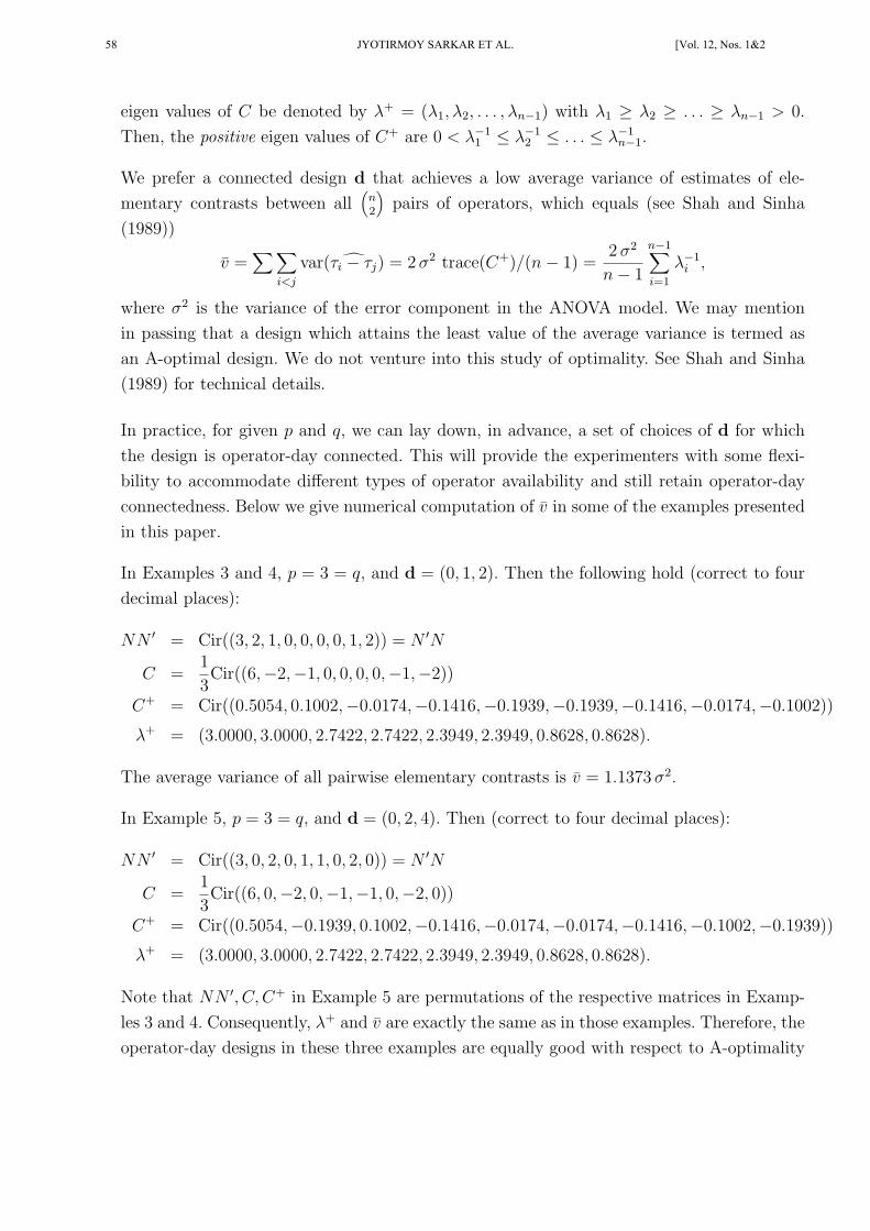
eigen values of C be denoted by λ+ = (λ1, λ2, . . . , λn−1) with λ1 ≥ λ2 ≥ . . . ≥ λn−1 > 0.

Then, the positive eigen values of C+ are 0 < λ−11 ≤ λ−1

2 ≤ . . . ≤ λ−1n−1.

We prefer a connected design d that achieves a low average variance of estimates of ele-

mentary contrasts between all(n2

)pairs of operators, which equals (see Shah and Sinha

(1989))

v̄ =∑∑

i<j

var( ̂τi − τj) = 2σ2 trace(C+)/(n− 1) =2 σ2

n− 1

n−1∑i=1

λ−1i ,

where σ2 is the variance of the error component in the ANOVA model. We may mention

in passing that a design which attains the least value of the average variance is termed as

an A-optimal design. We do not venture into this study of optimality. See Shah and Sinha

(1989) for technical details.

In practice, for given p and q, we can lay down, in advance, a set of choices of d for which

the design is operator-day connected. This will provide the experimenters with some flexi-

bility to accommodate different types of operator availability and still retain operator-day

connectedness. Below we give numerical computation of v̄ in some of the examples presented

in this paper.

In Examples 3 and 4, p = 3 = q, and d = (0, 1, 2). Then the following hold (correct to four

decimal places):

NN ′ = Cir((3, 2, 1, 0, 0, 0, 0, 1, 2)) = N ′N

C =1

3Cir((6,−2,−1, 0, 0, 0, 0,−1,−2))

C+ = Cir((0.5054, 0.1002,−0.0174,−0.1416,−0.1939,−0.1939,−0.1416,−0.0174,−0.1002))

λ+ = (3.0000, 3.0000, 2.7422, 2.7422, 2.3949, 2.3949, 0.8628, 0.8628).

The average variance of all pairwise elementary contrasts is v̄ = 1.1373σ2.

In Example 5, p = 3 = q, and d = (0, 2, 4). Then (correct to four decimal places):

NN ′ = Cir((3, 0, 2, 0, 1, 1, 0, 2, 0)) = N ′N

C =1

3Cir((6, 0,−2, 0,−1,−1, 0,−2, 0))

C+ = Cir((0.5054,−0.1939, 0.1002,−0.1416,−0.0174,−0.0174,−0.1416,−0.1002,−0.1939))

λ+ = (3.0000, 3.0000, 2.7422, 2.7422, 2.3949, 2.3949, 0.8628, 0.8628).

Note that NN ′, C, C+ in Example 5 are permutations of the respective matrices in Examp-

les 3 and 4. Consequently, λ+ and v̄ are exactly the same as in those examples. Therefore, the

operator-day designs in these three examples are equally good with respect to A-optimality


criterion. Note, however, that in Example 5 operators are allowed a day of rest in between

working days with no loss of efficiency in estimating their effects!

In Example 8, p = 5, q = 3, and d = (0, 1, 2). Then (correct to four decimal places):

NN ′ = Cir((3, 2, 1, 0, 0, 0, 0, 0, 0, 0, 0, 0, 0, 1, 2)) = N ′N

C =1

3Cir((6,−2,−1, 0, 0, 0, 0, 0, 0, 0, 0, 0, 0,−1,−2))

C+ = Cir((0.7610, 0.3447, 0.1937, 0.0139,−0.1156,−0.2169,−0.2833,−0.3167,

−0.3167,−0.2833,−0.2167,−0.1159, 0.0139, 0.1937, 0.3447))

λ+ = (3.0000, 3.0000, 2.8727, 2.8727, 2.7915, 2.7915, 2.6952, 2.6952,

2.1273, 2.1273, 1.1775, 1.1775, 0.3359, 0.3359).

The average variance of all pairwise elementary contrasts is v̄ = 1.6307σ2.

In Example 9, p = 5, q = 3, and d = (0, 2, 4). Then NN ′, C, C+ are permutations of the

respective matrices in Example 8. Consequently, λ+ and v̄ are exactly the same. Again, the

operator-day designs in Examples 8 and 9 are equally good with respect to A-optimality

criterion. Moreover, in Example 9 operators are allowed a day of rest in between working

days with no loss of efficiency in estimating their effects!

Similar calculations can be carried out for the general p×q CSDK designs. For the connected

design d = (0, 1, 2, . . . , q − 1), we compute v̄, the average variance of elementary contrasts

between all(n2

)pairs of operators for various values of p and q.

Table B1. Average variance v̄ of all(pq2

)elementary contrasts (×σ−2)

p\q 3 4 5 6 7 8 9

2 0.8967 0.6176 0.4717 0.3817 0.3206 0.2763 0.2428

3 1.1373 0.7437 0.5497 0.4348 0.3591 0.3056 0.2658

4 1.3813 0.8737 0.6305 0.4901 0.3993 0.3361 0.2898

5 1.6307 1.0051 0.7124 0.5461 0.4401 0.3672 0.3142

6 1.8792 1.1372 0.7948 0.6025 0.4812 0.3985 0.3389

7 2.1281 1.2696 0.8774 0.6591 0.5224 0.4299 0.3636

8 2.3773 1.4023 0.9603 0.7159 0.5638 0.4614 0.3884

9 2.6267 1.5351 1.0432 0.7727 0.6052 0.4929 0.4132


6. Acknowledgement We are thankful to the anonymous referee for carefully reading the

manuscript and offering necessary guidelines for the revision.

7. References

1. Bose, R.C., Shrikhande, S.S. and Parker, E.T. (1960). Further results on the construction

of mutually orthogonal Latin squares and the falsity of Euler’s conjecture. Canad. J.

Math. 12, 189-203.

2. Gray, R.M. (2006). Toeplitz and Circulant Matrices: A Review. Now Publishers Inc.

3. Kuhl, J.S. and Denley, T. (2012). A few remarks on avoiding partial Latin squares. Ars

Combinatoria, 106, 313-319.

4. Lorch, J.D. (2009). Mutually orthogonal families of linear Sudoku squares. Jour. Australas

Math. Soc. 87, 409-420.

5. — (2010). Orthogonal combings of linear Sudoku solutions. Australas J. Comb. 47, 247-

264.

6. — (2013). A quick construction of mutually orthogonal Sudoku squares. Private commu-

nication.

7. Pedersen, R.M. and Vis, T.L. (2009). Sets of mutually orthogonal Sudoku Latin squares.

College Math. Jour. 40, 174-180.

8. — and — (2012). The construction of a maximum set of Sudoku MOLS. Private Com-

munication.

9. Saba, F.A. and Sinha, B.K. (2014). SuDoKu as an experimental design—Beyond the

traditional Latin square design. Statistics and Applications. To appear.

10. Shah, K.R. and Sinha, B.K. (1989). Theory of Optimal Designs. Springer-Verlag Lecture

Notes in Statistics Series, 58.

11. Shah, K.R. and Sinha, B.K. (1996). Row-column designs. In: Design and Analysis of

Experiments. Handbook of Statistics, North-Holland, Amsterdam, Holland, 13, 903-

937.

12. Subramani, J. and Ponnuswamy, K.N. (2009). Construction and analysis of Sudoku

designs. Model Assisted Statistics and Applications, 4, 287-301.

13. Subramani, J. (2012). Construction of Graeco Sudoku square designs of odd order.

Bonfring International Journal of Data Mining, 2, 37-41.

__________________________________________________________________________________________________________________ Received: 10 June 2014; Revised: 19 September 2014; Accepted: 10 November 2014

variants of sudoku as useful experimental designsssca.org.in/media/4bksinha.pdfvariants of sudoku as...

Documents