variants of the adaptive large neighborhood search for the

THE INSTITUTE FOR SYSTEMS RESEARCH

ISR develops, applies and teaches advanced methodologies of design and analysis to solve complex, hierarchical, heterogeneous and dynamic prob-lems of engineering technology and systems for industry and government.

ISR is a permanent institute of the University of Maryland, within the A. James Clark School of Engineering. It is a graduated National Science

Foundation Engineering Research Center.

www.isr.umd.edu

Variants of the Adaptive Large Neighborhood Search for the Inventory Slack Routing Problem

Zijie Yan, Adam Montjoy, Jeffrey W. Herrmann

ISR TECHNICAL REPORT 2011-10

1

Variants of the Adaptive Large Neighborhood Search for the Inventory Slack Routing Problem

Zijie Yan Adam Montjoy

Jeffrey W. Herrmann September 7, 2011

Abstract

The inventory slack routing problem is a specialized vehicle routing problem that focuses on delivering waves of inventory to sites in a timely and even manner. It is difficult to find an optimal solution to this problem, thus heuristic and search techniques are necessary. This paper focuses on new variants of the Adaptive Large Neighborhood Search that incorporate new heuristics and linear programming to set delivery quantities. The search variants are tested on a set of instances to compare solution quality and computational effort.

1. Introduction

The Inventory Slack Routing Problem (ISRP) is a variant of the vehicle routing problem [1] in which material arrives at a central depot in multiple waves and must be delivered to sites that consume the material over a finite time horizon. The logistics objective is to deliver material as early as possible. In particular, management wishes the slack (earliness) of the deliveries to be as great as possible in order to reduce the likelihood that sites will not have material when it is needed. Like other vehicle routing problems, the ISRP is NP-‐hard, and heuristics and search algorithms are needed to find high-‐quality solutions in reasonable time.

2

Montjoy and Herrmann [2] described an Adaptive Large Neighborhood Search (ALNS) for finding solutions to the ISRP. Montjoy [3] discussed the performance of the search on a large set of problem instances. The search begins with an initial set of routes (determined by nearest neighbor-‐based heuristic) and iteratively destroys the current routes through removal heuristics and rebuilds the routes with insertion heuristics. In essence sites are removed and then reinserted into different routes based on how the minimum slack is changed. Depending on its performance, a heuristic’s probability of being chosen in future iterations is updated and its new solution is either accepted or rejected (or diversifies the search). None of the insertion heuristics tested previously employed a look-‐ahead characteristic. This paper introduces the regret insertion heuristic, which utilizes a look-‐ahead attribute, and tests this heuristic along with different ways to use linear programming to schedule the deliveries. The goal of the experiments is to determine whether adding the regret insertion heuristic makes the ALNS algorithm more efficient by analyzing the trade-‐off between computational effort and search performance.

2. Regret Insertion Heuristic

The regret insertion heuristic performs a search of the existing routes for the best route for each removed site that will result in the greatest minimum slack with a look ahead at potential future problems. The regret insertion heuristic finds, for each site and each vehicle, the position on that vehicle’s route that yields the greatest minimum slack. A site’s regret is the difference between the two greatest minimum slacks [4]. By prioritizing the removed sites that have the greatest regret, the algorithm hopes to avoid future problems by first inserting removed sites that have a great influence on minimum slack. (A site with little regret should have little impact on the minimum slack wherever it goes.)

The regret insertion heuristic starts with the existing vehicle routes and the removed sites. First, the procedure analyzes how many vehicles have no stops in their routes. Each of those vehicles will receive a removed site based on priority of which sites result in the highest minimum slack. The sites that are placed into a route are thus deleted from the set of removed sites. (It cannot improve the solution to have idle vehicles.) Next, the program determines the best routes for each remaining removed site by looking at the highest minimum slack calculated. The regret for each removed site is calculated by subtracting the second best route’s slack from the best route’s slack. The removed site with the highest regret is placed into its best route. This is repeated until no sites remain. This procedure is summarized in Figure 1.

Consider an instance with six sites and three vehicles and a partial solution with two removed sites. Vehicle 1 visits site 1, vehicle 2 visits site 2, and vehicle 3 visits sites 3 and 4. Sites 5 and 6 are unassigned.

3

The regret insertion heuristic tentatively inserts sites 5 and 6 into every vehicle route and the minimum slacks are saved. For example, when considering vehicle 3, the heuristic inserts each site before site 3, after site 3, and after site 4 in order to determine which location will result in the highest minimum slack.

The regret is calculated by the difference in slacks between the best route and second best route for each removed site. In this instance, the slack corresponding to each site and vehicle is shown in Table 1. For both sites 5 and 6, the route that has the most slack is vehicle 2, and the second best route is vehicle 3. The regret values are 2 and 8 for sites 5 and 6, respectively. The site with the largest regret is inserted first, so the heuristic adds site 6 to vehicle 2’s route. Then the process is repeated until no more removed sites remain.

By inserting the removed site with the highest regret first, the remaining removed site becomes easier to insert. If regret was not considered, site 5 would be added to the route for vehicle 2 because the previous algorithm deals with sites one at a time. Site 6 would then be inserted into vehicle 3 because that is the best remaining route. The highest minimum slack in the system would be 15, instead of the 21 calculated by regret.

Table 1. Minimum slack after insertion of sites 5 and 6 into vehicle routes.

Vehicle 1 Vehicle 2 Vehicle 3 Site 5 17 23 21 Site 6 13 23 15

4

Start

Are there vehicles with

no stops?

Insert a removed site with the highest minimum slack for

that route.

Yes

No

Yes No

Find the best position for the site based on highest

minimum slack

Yes

Yes

No

No

Choose one of the remaining removed sites

Choose one route

More routes?

More sites?

Calculate regret. Place removed site with highest regret into its best position.

More removed sites to insert? Done

Figure 1. Flowchart for the regret insertion heuristic.

5

3. Experimental Design

To analyze the performance of the ALNS with and without the regret insertion heuristic, we ran both versions of the ALNS on a set of 18 instances (see Table 2). These are a subset of the instances generated and tested by Montjoy [3]. Note that three instances have one set of nine sites, and another three instances a different set of nine sites. The key variables are heuristic performance (the average minimum slack of the best solution generated) and the computation time to run the search.

The original ALNS algorithm will be referred to as “ALNS.” For a complete description, including the values of the temperature and the cooling rate, see Montjoy [3]. The ALNS algorithm that incorporates the regret insertion heuristic will be denoted as “ALNSRR.” Refer to Table 7 for the labels for every algorithm.

Each trial of the ALNS completes 1500 iterations. Each trial of the ALNSR completes 1000 iterations. We ran 50 trials of each search on the instances with 5 to 50 sites but only 10 trials on the instances with 189 sites due to larger computational time.

The searches are run consecutively over the entire set of instances on one computer. The specifications of the computer used are Dell Optiplex 960 with Intel Core Duo CPU; E8400 @ 3.00 GHz; 2.99 GHz, 3.21 GB of RAM. The algorithms are coded and executed in MATLAB. The highest minimum slack per iteration, average times for every 100 iterations, standard deviations for every 100 iterations, time per iteration, average highest minimum slack for every 100 iterations, and the vehicle routes of the highest quality are all saved. The initial route is constructed by the nearest neighbor heuristic, ensuring that ALNS and ALNSR start at the same routes.

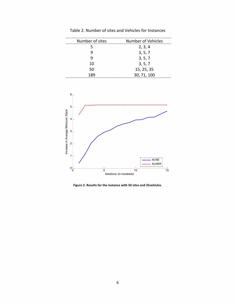
The difference in the number of iterations run for ALNS and ALNSR is based on the evidence gathered from initial testing that demonstrated that 1500 iterations for ALNSR is wasteful and inefficient as the algorithm will most likely find the best solution before then. One sample is taken from an instance of 50 sites and 35 vehicles.

As shown in Figures 2 and 3, the ALNSR found the best solution well under the 1000 or 1500 iterations specified on the instance with 50 sites and 35 vehicles. Clearly, it is unnecessary to run 1500 iterations for the ALNSR, whereas ALNS requires 1500 iterations to get close to the best found solution.

Only in the large instances with 189 sites are both 1500 and 1000 iterations for ALNS and ALNSR, respectively, not enough. This will be discussed in more detail later.

6

Table 2. Number of sites and Vehicles for Instances

Number of sites Number of Vehicles 5 2, 3, 4 9 3, 5, 7 9 3, 5, 7 10 3, 5, 7 50 15, 25, 35 189 30, 71, 100

0 5 10 150

1

2

3

4

5

6

Iterations (in hundreds)

Incr

ease

in A

vera

ge M

inim

um S

lack

ALNSALNSR

Figure 2. Results for the instance with 50 sites and 35vehicles.

7

0 5 10 150

0.5

1

1.5

2

2.5

3

3.5

4

4.5

5


Incr

ease

in A

vera

ge M

inim

um S

lack

ALNSALNSR

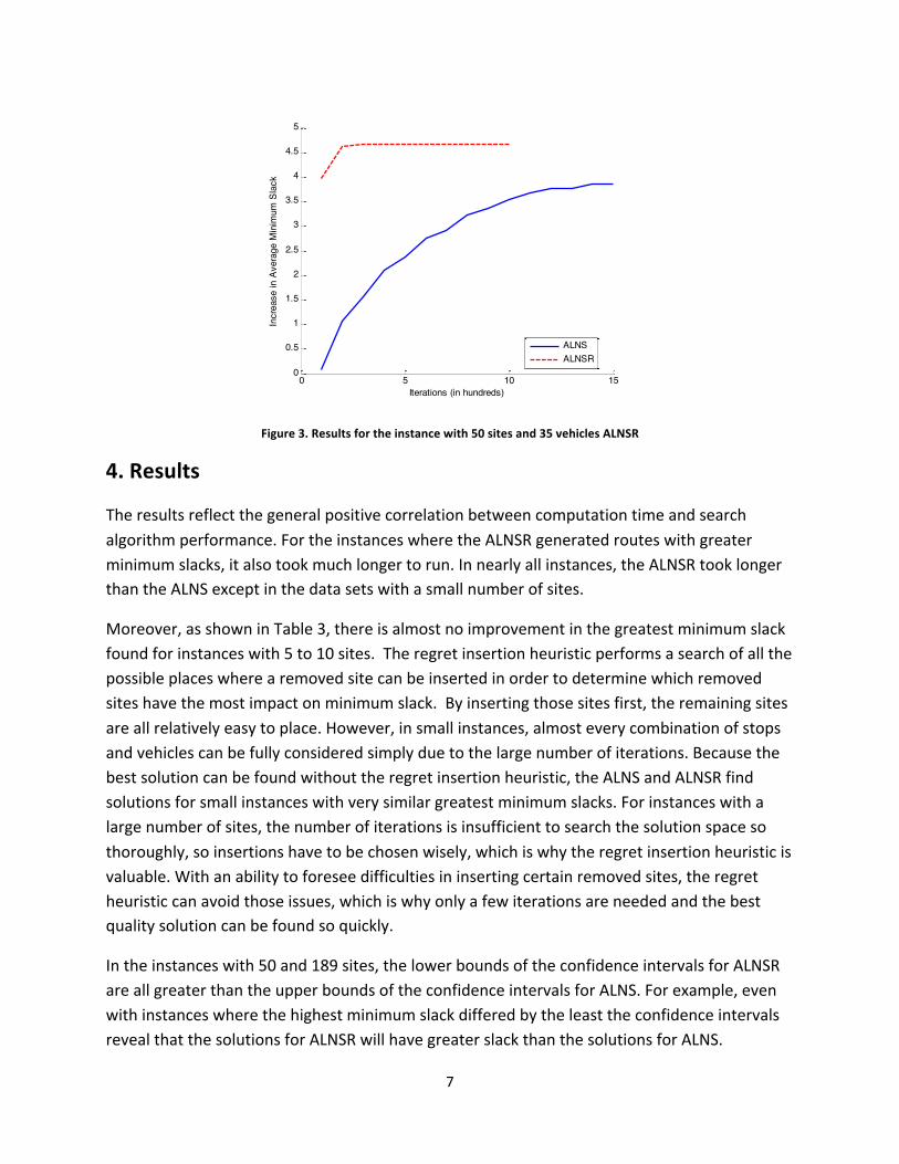
Figure 3. Results for the instance with 50 sites and 35 vehicles ALNSR

4. Results

The results reflect the general positive correlation between computation time and search algorithm performance. For the instances where the ALNSR generated routes with greater minimum slacks, it also took much longer to run. In nearly all instances, the ALNSR took longer than the ALNS except in the data sets with a small number of sites.

Moreover, as shown in Table 3, there is almost no improvement in the greatest minimum slack found for instances with 5 to 10 sites. The regret insertion heuristic performs a search of all the possible places where a removed site can be inserted in order to determine which removed sites have the most impact on minimum slack. By inserting those sites first, the remaining sites are all relatively easy to place. However, in small instances, almost every combination of stops and vehicles can be fully considered simply due to the large number of iterations. Because the best solution can be found without the regret insertion heuristic, the ALNS and ALNSR find solutions for small instances with very similar greatest minimum slacks. For instances with a large number of sites, the number of iterations is insufficient to search the solution space so thoroughly, so insertions have to be chosen wisely, which is why the regret insertion heuristic is valuable. With an ability to foresee difficulties in inserting certain removed sites, the regret heuristic can avoid those issues, which is why only a few iterations are needed and the best quality solution can be found so quickly.

In the instances with 50 and 189 sites, the lower bounds of the confidence intervals for ALNSR are all greater than the upper bounds of the confidence intervals for ALNS. For example, even with instances where the highest minimum slack differed by the least the confidence intervals reveal that the solutions for ALNSR will have greater slack than the solutions for ALNS.

8

Table 3. Comparison of ALNS and ALNSR Search Quality over 18 Instances

Number of sites

Number of Vehicles

Average Greatest Minimum Slack

ALNS ALNSR

95% Confidence Interval on Greatest Minimum Slack ALNS ALNSR

5 2 478.5 478.5 [478.5 478.5] [478.5 478.5] 3 491.5 491.5 [491.5 491.5] [491.5 491.5] 4 491.5 491.5 [491.5 491.5] [491.5 491.5]

9 (F) 3 1281.0 1280.9 [1280.9 1281.0] [1280.9 1281.0] 5 1316.0 1316.0 [1316.0 1316.0] [1316.0 1316.0] 7 1328.0 1328.0 [1328.0 1328.0] [1328.0 1328.0]

9 (C) 3 458.0 458.0 [458.0 458.0] [458.0 458.0] 5 482.7 482.9 [482.4 482.8] [482.8 483.0] 7 496.0 496.0 [496.0 496.0] [496.0 496.0] 10 3 1082.3 1082.9 [1082.1 1082.6] [1082.8 1083.0] 5 1092.2 1092.1 [1092.1 1092.2] [1092.1 1092.2] 7 1092.2 1092.2 [1092.2 1092.2] [1092.2 1092.2] 50 15 1248.1 1266.0 [1246.4 1249.7] [1264.8 1267.1] 25 1284.1 1285.1 [1283.7 1284.5] [1284.9 1285.2] 35 1284.4 1285.2 [1284.4 1284.9] [1285.2 1285.2]

189 30 1247.1 1266.9 [1245.9 1248.3] [1265.5 1268.3] 71 1319.8 1335.7 [1319.3 1320.3] [1334.7 1336.7] 100 1332.4 1345.5 [1331.5 1333.3] [1344.3 1346.7]

9

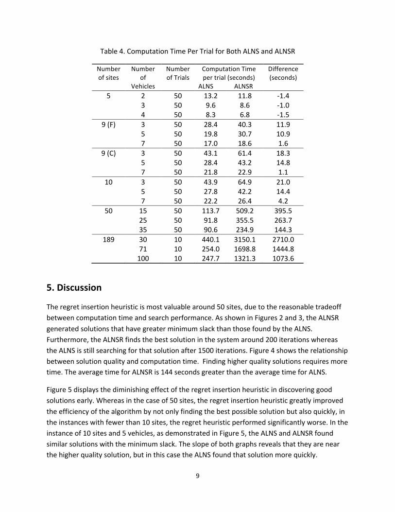
Table 4. Computation Time Per Trial for Both ALNS and ALNSR

Number of sites

Number of

Vehicles

Number of Trials

Computation Time per trial (seconds)

ALNS ALNSR

Difference (seconds)

5 2 50 13.2 11.8 -‐1.4 3 50 9.6 8.6 -‐1.0 4 50 8.3 6.8 -‐1.5

9 (F) 3 50 28.4 40.3 11.9 5 50 19.8 30.7 10.9 7 50 17.0 18.6 1.6

9 (C) 3 50 43.1 61.4 18.3 5 50 28.4 43.2 14.8 7 50 21.8 22.9 1.1 10 3 50 43.9 64.9 21.0 5 50 27.8 42.2 14.4 7 50 22.2 26.4 4.2 50 15 50 113.7 509.2 395.5 25 50 91.8 355.5 263.7 35 50 90.6 234.9 144.3

189 30 10 440.1 3150.1 2710.0 71 10 254.0 1698.8 1444.8 100 10 247.7 1321.3 1073.6

5. Discussion

The regret insertion heuristic is most valuable around 50 sites, due to the reasonable tradeoff between computation time and search performance. As shown in Figures 2 and 3, the ALNSR generated solutions that have greater minimum slack than those found by the ALNS. Furthermore, the ALNSR finds the best solution in the system around 200 iterations whereas the ALNS is still searching for that solution after 1500 iterations. Figure 4 shows the relationship between solution quality and computation time. Finding higher quality solutions requires more time. The average time for ALNSR is 144 seconds greater than the average time for ALNS.

Figure 5 displays the diminishing effect of the regret insertion heuristic in discovering good solutions early. Whereas in the case of 50 sites, the regret insertion heuristic greatly improved the efficiency of the algorithm by not only finding the best possible solution but also quickly, in the instances with fewer than 10 sites, the regret heuristic performed significantly worse. In the instance of 10 sites and 5 vehicles, as demonstrated in Figure 5, the ALNS and ALNSR found similar solutions with the minimum slack. The slope of both graphs reveals that they are near the higher quality solution, but in this case the ALNS found that solution more quickly.

10

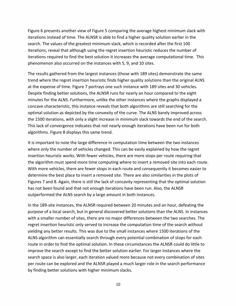
Figure 6 presents another view of Figure 5 comparing the average highest minimum slack with iterations instead of time. The ALNSR is able to find a higher quality solution earlier in the search. The values of the greatest minimum slack, which is recorded after the first 100 iterations, reveal that although using the regret insertion heuristic reduces the number of iterations required to find the best solution it increases the average computational time. This phenomenon also occurred on the instances with 5, 9, and 10 sites.

The results gathered from the largest instances (those with 189 sites) demonstrate the same trend where the regret insertion heuristic finds higher quality solutions than the original ALNS at the expense of time. Figure 7 portrays one such instance with 189 sites and 30 vehicles. Despite finding better solutions, the ALNSR runs for nearly an hour compared to the eight minutes for the ALNS. Furthermore, unlike the other instances where the graphs displayed a concave characteristic, this instance reveals that both algorithms are still searching for the optimal solution as depicted by the convexity of the curve. The ALNS barely improved across the 1500 iterations, with only a slight increase in minimum slack towards the end of the search. This lack of convergence indicates that not nearly enough iterations have been run for both algorithms. Figure 8 displays this same trend.

It is important to note the large difference in computation time between the two instances where only the number of vehicles changed. This can be easily explained by how the regret insertion heuristic works. With fewer vehicles, there are more stops per route requiring that the algorithm must spend more time computing where to insert a removed site into each route. With more vehicles, there are fewer stops in each route and consequently it becomes easier to determine the best place to insert a removed site. There are also similarities in the plots of Figures 7 and 8. Again, there is still the lack of concavity representing that the optimal solution has not been found and that not enough iterations have been run. Also, the ALNSR outperformed the ALNS search by a large amount in both instances.

In the 189-‐site instances, the ALNSR required between 20 minutes and an hour, defeating the purpose of a local search, but in general discovered better solutions than the ALNS. In instances with a smaller number of sites, there are no major differences between the two searches. The regret insertion heuristic only served to increase the computation time of the search without yielding any better results. This was due to the small instances where 1500 iterations of the ALNS algorithm can essentially search through every potential combination of stops for each route in order to find the optimal solution. In these circumstances the ALNSR could do little to improve the search except to find the better solution earlier. For larger instances where the search space is also larger, each iteration valued more because not every combination of sites per route can be explored and the ALNSR played a much larger role in the search performance by finding better solutions with higher minimum slacks.

11

0 50 100 150 200 2500

1

2

3

4

5

6

Time (in seconds)

Incr

ease

in A

vera

ge M

inim

um S

lack

ALNSALNSR

Figure 4. Results for 50 sites and 35 vehicles

0 5 10 15 20 25 30 35 40 450

0.2

0.4

0.6

0.8

1

1.2

1.4

1.6

1.8

Time (in seconds)

Incr

ease

in A

vera

ge M

inim

um S

lack

ALNSALNSR


12

0 5 10 150

0.2

0.4

0.6

0.8

1

1.2

1.4

1.6

1.8


Incr

ease

in A

vera

ge M

inim

um S

lack

ALNSALNSR


0 500 1000 1500 2000 2500 3000 35000

5

10

15

20

25

Time (in seconds)

Incr

ease

in A

vera

ge M

inim

um S

lack

ALNSALNSR


13

0 200 400 600 800 1000 1200 1400 1600 18000

2

4

6

8

10

12

14

16

18

Time (in seconds)

Incr

ease

in A

vera

ge M

inim

um S

lack

ALNSALNSR


6. Calculating Regret using Route Durations

The regret insertion heuristic increased the computation time of the search greatly. Even though it is able to discover higher quality solutions, this increased effort makes the algorithm inefficient. Determining the delivery quantities and calculating the minimum slack for each possible location for a removed site takes significant time. Because the minimum slack largely depends upon the route durations, we considered a version of the regret insertion heuristic that considered the difference in vehicle route durations. In this version, a removed site is inserted into every possible location in a route. At each location, the heuristic considers the total route duration. Then the removed site with the greatest regret – difference in route durations between its best route and second best route – is inserted first.

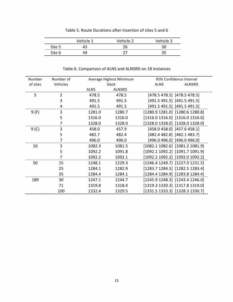
Consider again the example instance discussed before. Table 5 lists the route durations that result from adding each site to each vehicle’s route.

The regret is calculated by the difference in travel times between the best and second best route for each removed site. The shortest route for both sites 5 and 6 is vehicle 2, and the second best route is vehicle 3. The regret values are 4 and 8 for sites 5 and 6, respectively. The site with the largest regret is inserted first, so site 6 is added to vehicle 2’s route. Then the process is repeated until no more removed sites remain.

The ALNS search with the modified regret insertion heuristic will be denoted by “ALNSRD.”

As shown in Table 6, compared to the solutions generated by the ALNS, the solutions found by the ALNSRD for the instances with 5 and 9 sites had the same quality. For the larger instances,

14

the solutions found by the ALNSRD were not as good. The performance of the ALNSRD was particularly poor on the instance with 50 sites and 15 vehicles.

As shown in Table 9, the ALNSRD did require less computation time than the other searches and reduced the time in some instances by nearly 50%. Like the search performances of ALNSR, ALNSRD finds the same solutions as ALNS in smaller sized instances but as the size of the sites increase the differences become more apparent.

Looking at each vehicle’s routes for various instances, ALNSRD does not find the same routes as ALNS nor ALNSR. This can be attributed to the fact that ALNSRD seeks solely to minimize the travel times per vehicle instead of maximizing the minimum slack. Even though the vehicle routes vary, the minimum slacks differ only very slightly. The small differences can be logically explained by the strong correlation between slacks and travel times. Manipulating travel time will directly affect slack.

Though the ALNSRD could not find solutions of the same quality as ALNS or ALNSR, it was able to finish its search in much shorter time. The results indicated unexpected behavior as we predicted the ALNSRD will still take longer time than ALNS to complete. However, because slack was no longer calculated, thousands of calls to our delivery volume improvement (DVI) function was removed which sped up the search considerably. The reason why ALNSRD ran faster than ALNS was due to the adaptive nature of the search. Heuristics that find better solutions are more likely to be called again. Since the regret insertion heuristic is able to discover higher quality solutions, it becomes used more than the other insertion heuristics Moreover, the new regret insertion heuristic runs very quickly because it makes no call to external functions unlike the other insertion heuristics. The ALNSRD calls the regret insertion heuristic more as the search progresses due to its effectiveness and speeds up the search as less attention is diverted to the more time consuming insertion heuristics.

The ALNSRD does not perform as well as ALNS and ALNSR. Figure 9 captures the limitations of the new regret insertion heuristic in finding as good of a solution as ALNS or ALNSR. However, the short amount of computation time is evident.

In the medium sized instances where ALNSR greatly outperformed ALNS, ALNSRD fails to maintain the same results.

Figure 10 reveals the similar increase in average minimum slack between ALNS and ALNSRD. Both algorithms performed similarly, revealing that the new regret insertion heuristic has little to no effect of improving the search quality. The ALNSR is simply better than both ALNS and ALNSRD although it does take much longer to run.

15

Table 5. Route Durations after Insertion of sites 5 and 6

Vehicle 1 Vehicle 2 Vehicle 3 Site 5 43 26 30 Site 6 49 27 35

Table 6. Comparison of ALNS and ALNSRD on 18 Instances

Number of sites

Number of Vehicles

Average Highest Minimum Slack

ALNS ALNSRD

95% Confidence Interval ALNS ALNSRD

5 2 478.5 478.5 [478.5 478.5] [478.5 478.5] 3 491.5 491.5 [491.5 491.5] [491.5 491.5] 4 491.5 491.5 [491.5 491.5] [491.5 491.5]

9 (F) 3 1281.0 1280.7 [1280.9 1281.0] [1280.6 1280.8] 5 1316.0 1316.0 [1316.0 1316.0] [1316.0 1316.0] 7 1328.0 1328.0 [1328.0 1328.0] [1328.0 1328.0]

9 (C) 3 458.0 457.9 [458.0 458.0] [457.6 458.1] 5 482.7 482.4 [482.4 482.8] [482.1 483.7] 7 496.0 496.0 [496.0 496.0] [496.0 496.0] 10 3 1082.3 1081.5 [1082.1 1082.6] [1081.2 1081.9] 5 1092.2 1091.8 [1092.1 1092.2] [1091.7 1091.9] 7 1092.2 1092.1 [1092.2 1092.2] [1092.0 1092.2] 50 15 1248.1 1229.3 [1246.4 1249.7] [1227.0 1231.5] 25 1284.1 1282.9 [1283.7 1284.5] [1282.5 1283.4] 35 1284.4 1284.1 [1284.4 1284.9] [1283.8 1284.4]

189 30 1247.1 1244.7 [1245.9 1248.3] [1243.4 1246.0] 71 1319.8 1318.4 [1319.3 1320.3] [1317.8 1319.0] 100 1332.4 1329.5 [1331.5 1333.3] [1328.3 1330.7]

16

0 5 10 15 20 25 30 35 40 450

0.2

0.4

0.6

0.8

1

1.2

1.4

1.6

1.8

2

Time (in seconds)

Incr

ease

in A

vera

ge M

inim

um S

lack

ALNSALNSRALNSRD


0 50 100 150 200 2500

1

2

3

4

5

6

Time (in seconds)

Incr

ease

in A

vera

ge M

inim

um S

lack

ALNSALNSRALNSRD

Figure 10. Comparison of ALNS, ALNSR, and ALNSRD for the instance with 50 sites and 35 vehicles.

7. Adding Linear Programming to ALNS

The ALNS, ALNSR, and ALNSRD searches used delivery volume improvement (DVI) to improve the delivery quantities of each vehicle. The DVI procedure considers each vehicle separately. In order to determine the best minimum slack for a given set of routes by optimizing the delivery quantities of all vehicles simultaneously, we formulated an appropriate linear program (LP).

17

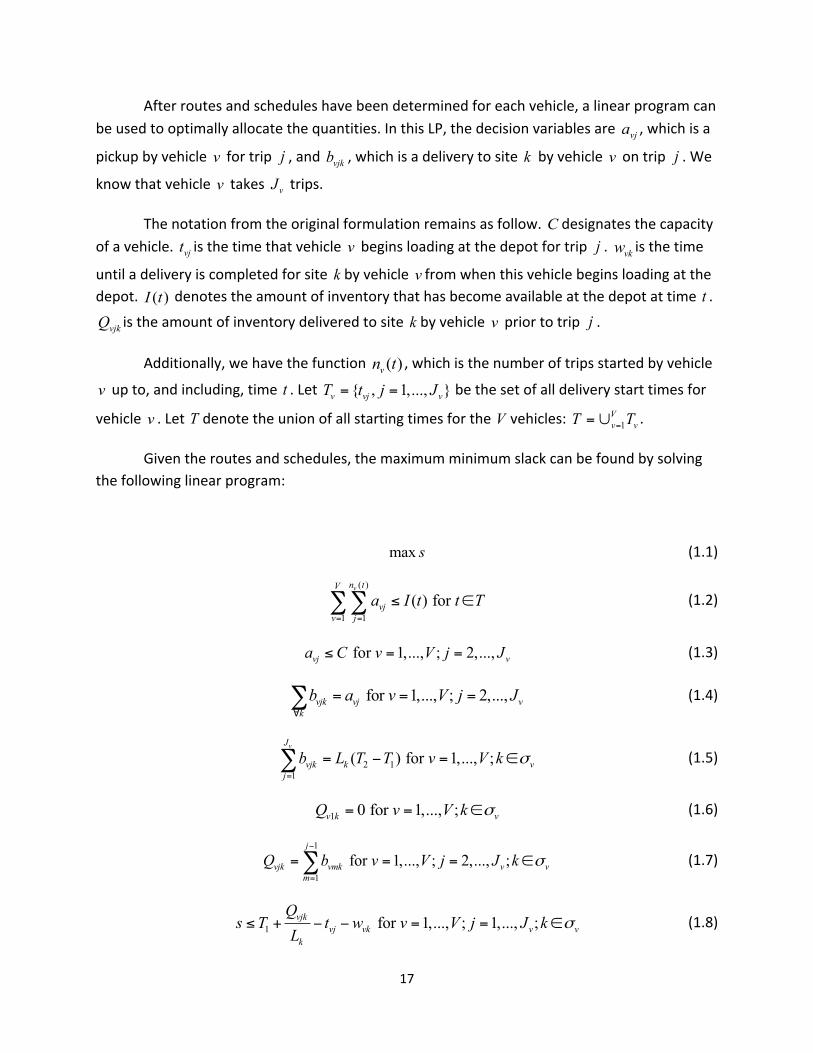
After routes and schedules have been determined for each vehicle, a linear program can be used to optimally allocate the quantities. In this LP, the decision variables are vja , which is a

pickup by vehicle v for trip j , and vjkb , which is a delivery to site k by vehicle v on trip j . We

know that vehicle v takes vJ trips.

The notation from the original formulation remains as follow. C designates the capacity of a vehicle. vjt is the time that vehicle v begins loading at the depot for trip j . vkw is the time

until a delivery is completed for site k by vehicle v from when this vehicle begins loading at the depot. ( )I t denotes the amount of inventory that has become available at the depot at time t .

vjkQ is the amount of inventory delivered to site k by vehicle v prior to trip j .

Additionally, we have the function ( )vn t , which is the number of trips started by vehicle

v up to, and including, time t . Let { , 1,..., }v vj vT t j J= = be the set of all delivery start times for

vehicle v . Let T denote the union of all starting times for the V vehicles: 1Vv vT T==∪ .

Given the routes and schedules, the maximum minimum slack can be found by solving the following linear program:

max s (1.1)

( )

1 1( ) for

vn tV

vjv j

a I t t T= =

≤ ∈∑∑ (1.2)

for 1,..., ; 2,...,vj va C v V j J≤ = = (1.3)

for 1,..., ; 2,...,vjk vj vkb a v V j J

∀

= = =∑ (1.4)

2 11

( ) for 1,..., ;vJ

vjk k vjb L T T v V k σ

=

= − = ∈∑ (1.5)

1 0 for 1,..., ;v k vQ v V k σ= = ∈ (1.6)

1

1 for 1,..., ; 2,..., ;

j

vjk vmk v vm

Q b v V j J k σ−

=

= = = ∈∑ (1.7)

1 for 1,..., ; 1,..., ;vjkvj vk v v

k

Qs T t w v V j J k

Lσ≤ + − − = = ∈ (1.8)

18

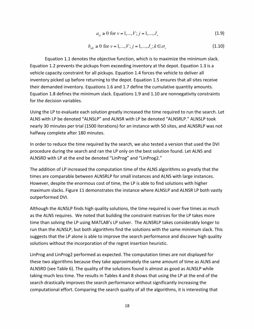
0 for 1,..., ; 1,...,vj va v V j J≥ = = (1.9)

0 for 1,..., ; 1,..., ;vjk v vb v V j J k σ≥ = = ∈ (1.10)

Equation 1.1 denotes the objective function, which is to maximize the minimum slack. Equation 1.2 prevents the pickups from exceeding inventory at the depot. Equation 1.3 is a vehicle capacity constraint for all pickups. Equation 1.4 forces the vehicle to deliver all inventory picked up before returning to the depot. Equation 1.5 ensures that all sites receive their demanded inventory. Equations 1.6 and 1.7 define the cumulative quantity amounts. Equation 1.8 defines the minimum slack. Equations 1.9 and 1.10 are nonnegativity constraints for the decision variables.

Using the LP to evaluate each solution greatly increased the time required to run the search. Let ALNS with LP be denoted “ALNSLP” and ALNSR with LP be denoted “ALNSRLP.” ALNSLP took nearly 30 minutes per trial (1500 iterations) for an instance with 50 sites, and ALNSRLP was not halfway complete after 180 minutes.

In order to reduce the time required by the search, we also tested a version that used the DVI procedure during the search and ran the LP only on the best solution found. Let ALNS and ALNSRD with LP at the end be denoted “LinProg” and “LinProg2.”

The addition of LP increased the computation time of the ALNS algorithms so greatly that the times are comparable between ALNSRLP for small instances and ALNS with large instances. However, despite the enormous cost of time, the LP is able to find solutions with higher maximum slacks. Figure 11 demonstrates the instance where ALNSLP and ALNSR LP both vastly outperformed DVI.

Although the ALNSLP finds high quality solutions, the time required is over five times as much as the ALNS requires. We noted that building the constraint matrices for the LP takes more time than solving the LP using MATLAB’s LP solver. The ALNSRLP takes considerably longer to run than the ALNSLP, but both algorithms find the solutions with the same minimum slack. This suggests that the LP alone is able to improve the search performance and discover high quality solutions without the incorporation of the regret insertion heuristic.

LinProg and LinProg2 performed as expected. The computation times are not displayed for these two algorithms because they take approximately the same amount of time as ALNS and ALNSRD (see Table 6). The quality of the solutions found is almost as good as ALNSLP while taking much less time. The results in Tables 4 and 8 shows that using the LP at the end of the search drastically improves the search performance without significantly increasing the computational effort. Comparing the search quality of all the algorithms, it is interesting that

19

LinProg performs the best in the shortest amount of time. Not only does it take less time than ALNSR, but it also outperforms it for the instances with 10 and 50 sites.

Table 7. Table of Algorithm Labels

Label Corresponding Algorithm ALNS Original ALNS ALNSR ALNS with regret insertion

heuristic ALNSRD ALNS with modified regret

insertion heuristic based on route duration

ALNSLP ALNS with linear programming replacing DVI

ALNSRLP ALNSR with linear programming replacing DVI

LinProg Linear programming run once after ALNS finishes

LinProg2 Linear programming run once after ALNSRD finishes

Table 8. Comparison of ALNSLP and ALNSRLP.

Number of sites

Number of Vehicles

Greatest Minimum Slack Average

ALNSLP ALNSRLP

Greatest Minimum Slack 95% Confidence Interval

ALNSLP ALNSRLP 5 2 483.7 483.7 [483.7 483.7] [483.7 483.7] 3 493.8 493.8 [493.8 493.8] [493.8 493.8] 4 498.1 498.1 [498.1 498.1] [498.1 498.1]

9 (F) 3 1280.9 1281.0 [1280.8 1281.0] [1280.9 1281.0] 5 1316.0 1316.0 [1316.0 1316.0] [1316.0 1316.0] 7 1328.0 1328.0 [1328.0 1328.0] [1328.0 1328.0]

9 (C) 3 458.0 458.0 [458.0 458.0] [458.0 458.0] 5 482.4 483.0 [482.1 482.6] [482.9 483.0] 7 496.0 496.0 [496.0 496.0] [496.0 496.0] 10 3 1084.7 1084.7 [1084.7 1084.7] [1084.7 1084.7] 5 1096.8 1096.8 [1096.8 1096.8] [1096.8 1096.8] 7 1101.0 1101.1 [1101.0 1101.0] [1101.1 1101.1]

20

Table 9. Comparison of LinProg and LinProg2.

Number of sites

Number of Vehicles

Average Highest Minimum Slack

LinProg LinProg2

95% Confidence Interval LinProg LinProg2

5 2 478.6 478.6 [478.6 478.6] [478.6 478.6] 3 493.8 493.8 [493.8 493.8] [493.8 493.8] 4 497.5 497.5 [497.5 497.5] [497.5 497.5]

9 (F) 3 1280.9 1280.7 [1280.8 1281.0] [1280.5 1281.0] 5 1316.0 1316.0 [1316.0 1316.0] [1316.0 1316.0] 7 1328.0 1328.0 [1328.0 1328.0] [1328.0 1328.0]

9 (C) 3 458.0 458.0 [458.0 458.0] [458.0 458.0] 5 482.6 482.2 [482.2 483.1] [481.6 482.8] 7 496.0 496.0 [496.0 496.0] [496.0 496.0] 10 3 1083.3 1082.8 [1082.8 1083.7] [1082.1 1083.6] 5 1095.0 1094.9 [1095.0 1095.1] [1094.7 1095.1] 7 1100.1 1100.1 [1100.1 1100.2] [1099.9 1100.2] 50 15 1263.2 1251.6 [1259.3 1267.2] [1247.2 1256.0] 25 1292.9 1292.9 [1292.4 1293.4] [1292.3 1293.4] 35 1297.4 1297.3 [1296.9 1297.8] [1296.9 1297.8]

189 30 1245.3 1244.0 [1244.5 1246.1] [1244.0 1244.0] 71 1318.9 1319.0 [1318.2 1319.6] [1318.0 1318.0] 100 1332.9 1329.0 [1331.3 1334.5] [1328.0 1330.0]

21

Table 10. Computation Time per Trial for ALNS, ALNSR, ALNSRD, ALNSLP, and ALNSRLP.

Number of sites

Number of

Vehicles

Number of Trials

Computation Time per trial (seconds)

ALNS ALNSR ALNSRD ALNSLP ALNSRLP 5 2 50 13.2 11.8 8.1 82.3 78.9 3 50 9.6 8.6 6.1 55.3 58.1 4 50 8.3 6.8 5.5 38.8 40.7

9 (F) 3 50 28.4 40.3 19.0 190.2 312.7 5 50 19.8 30.7 12.8 175.8 364.0 7 50 17.0 18.6 11.1 127.4 233.6

9 (C) 3 50 43.1 61.4 28.9 327.9 531.6 5 50 28.4 43.2 19.3 227.4 462.2 7 50 21.8 22.9 15.1 144.8 247.1 10 3 50 43.9 64.9 27.8 234.6 381.0 5 50 27.8 42.2 17.8 161.2 335.7 7 50 22.2 26.4 13.7 111.9 227.6 50 15 50 113.7 509.2 74.2 25 50 91.8 355.5 61.5 35 50 90.6 234.9 60.8

189 30 10 440.1 3150.1 288.2 71 10 254.0 1698.8 171.6 100 10 247.7 1321.3 169.4

0 50 100 150 200 2500

1

2

3

4

5

6

7

8

9

10

Time (in seconds)

Incr

ease

in A

vera

ge M

inim

um S

lack

ALNSALNSRALNSLPALNSRLP

Figure 11. Comparison of ALNS, ALNSR, ALNSLP, ALNSRLP for the instance with 10 sites and 7 vehicles.

22

8. Conclusions

The regret insertion heuristic performs the most efficiently in instances with less than 50 sites. There is almost no difference in search performance between ALNS and ALNSR for instances with a small number of sites. On the other hand, for instances with a large number of sites there were significant improvements in solution quality for ALNSR. However, the increase in quality comes at the cost of an immense computational time. For the instances with 50 sites, the ALNSR not only finds higher quality solutions but also does so within a reasonable amount of time. The regret insertion heuristic is inefficient in instances with a large or small number of sites, but around the range of 50 sites it performs exceptionally well both in finding high quality solutions and early.

With the implementation of the new regret insertion heuristic, the ALNSR becomes less favorable for small instances. The ALNSRD finds the same solutions as ALNS and ALNSR but much faster.

The addition of the LP algorithm greatly increased the search performance of the ALNS. The solutions were all of higher quality than those found with ALNS. ALNSLP and ALNSRLP found similar results despite the ALNSRLP requiring longer computation time, suggesting that the regret insertion heuristic only slows down the search without generating better results. The LinProg and LinProg2 are the best algorithms out of the instances tested. They not only find higher quality solutions than ALNS and ALNSR, they also take a short amount of time to run. This suggests that the removal and insertion heuristics with DVI are competent in finding high quality routes and the LP can optimize the minimum slacks through efficient scheduling.

Acknowledgements

This publication was supported by Award Number 1H75TP000309 from the CDC to NACCHO. Its contents are solely the responsibility of the University of Maryland and do not necessarily represent the official views of CDC or NACCHO.

References

[1] Campbell, A.M., Clarke, L.W., and Savelsbergh, M.W.P. (2001) The Vehicle Routing Problem, Society for Industrial and Applied Mathematics, Philadelphia, PA.

[2] Montjoy, A., and J.W. Herrmann. Adaptive Large Neighborhood Search for the Inventory Slack Routing Problem. Industrial Engineering Research Conference, Cancun, Mexico, 2010.

[3] Montjoy, A. Solving the Inventory Slack Routing Problem for Emergency Medication Distribution. Master’s thesis, Department of Mechanical Engineering, University of Maryland, 2010.

23

[4] Pisinger , D., Ropke, S. A general heuristic for vehicle routing problems, Computers and Operations Research, v.34 n.8, p.2403-‐2435, August, 2007 [doi>10.1016/j.cor.2005.09.012]

variants of the adaptive large neighborhood search for the

Documents